Versatile Robust Clustering of Ad Hoc Cognitive Radio Network

Abstract

Cluster structure in cognitive radio networks facilitates cooperative spectrum sensing, routing and other functionalities. The unlicensed channels, which are available for every member of a group of cognitive radio users, consolidate the group into a cluster, and the availability of unlicensed channels decides the robustness of that cluster against the licensed users’ influence. This paper analyses the problem that how to form robust clusters in cognitive radio network, so that more cognitive radio users can get benefits from cluster structure even when the primary users’ operation are intense. We provide a formal description of robust clustering problem, prove it to be NP-hard and propose a centralized solution, besides, a distributed solution is proposed to suit the dynamics in the ad hoc cognitive radio network. Congestion game model is adopted to analyse the process of cluster formation, which not only contributes designing the distributed clustering scheme directly, but also provides the guarantee of convergence into Nash Equilibrium and convergence speed. Our proposed clustering solution is versatile to fulfill some other requirements such as faster convergence and cluster size control. The proposed distributed clustering scheme outperforms the related work in terms of cluster robustness, convergence speed and overhead. The extensive simulation supports our claims.

1 Introduction

Cognitive radio (CR) is a promising technology to solve the spectrum scarcity problem [1]. Licensed users access the spectrum allocated to them whenever there is information to be transmitted. In contrast, as one way, unlicensed users can access the spectrum via opportunistic spectrum access, i.e., they access the licensed spectrum only after validating the channel is unoccupied by licensed users, where spectrum sensing [2] plays an important role in this process. In this hierarchical spectrum access model [3], the licensed users are also called primary users (PU), while the unlicensed users are referred to as secondary users and constitute a so called cognitive radio network (CRN). Regarding the operation of CRN, efficient spectrum sensing is identified to be critical for a smooth operation of a cognitive radio network [4]. This can be achieved by cooperative spectrum sensing of multiple secondary users, which has been shown to cope effectively with noise uncertainty and channel fading, thus remarkably improving the sensing accuracy [5]. Collaborative sensing relies on the consensus of CR users within a certain area, in this regard, clustering is regarded as an effective method to realize cooperative spectrum sensing [6, 7]. Clustering is a process of grouping certain users in a proximity into a collective. Clustering is also efficient to coordinate the channel switch operation when primary users are detected by at least one CR node residing in the cluster. The cluster head can enable all the CR devices within the same cluster to stop payload transmission swiftly on the operating channel and to vacate the channel  [8]. In addition to the collaborate sensing advantage, the use of clusters is beneficial as it reduces the interference between cognitive clusters [9]. Clustering algorithm has also been proposed to support routing in cognitive radio networks  [10].

Clusters are formed in the very beginning of the network operation, and re-formed periodically according to the dynamics of the CRN. Each formed cluster has one or multiple unlicensed channels which are available for every CR node in the cluster. The available unlicensed channels are referred to in the following of this paper as common licensed channels (or common channels for short, which is abbreviated as CC). Both payload and control overheads can be transmitted on the CCs. When one or several cluster members can not access one certain CC on which primary user activity is detected, the channel will be excluded from the set of CCs. In particular, if that channel is being used for payload communication, the communication pair will stop and resume the transmission on another available channel from CCs. The availability of CCs within a cluster defines the existence of that cluster, i.e., no CCs are available means the corresponding cluster doesn’t exist. In the context of CRN, the activity of primary users is usually unknown to the secondary users, thus when the primary users’ activity is deemed as random, the cluster which secures more CCs will anticipate a longer time span. It is obvious that fewer members in a cluster yield more CCs, but obtaining more CCs by decreasing the cluster size contradicts to the motivation of clustering, i.e., benefit the cluster members with cooperative decision making. For example, spectrum sensing accuracy coralates with the cluster size [11], and power consumption doesn’t favor small clusters [12, 13]. In this paper the robustness of clusters means the ability of the clusters to sustain the increasing activity of primary users.

There has been a lot of research done for clustering in wireless networks. In ad-hoc and mesh networks, the major goal of clustering is to maximize connectivity or to improve the performance of routes [14, 15]. The emphasis of clustering in sensor networks is on network lifetime and coverage [10]. In respect of CRN, [7, 16, 17] propose the clustering schemes to form clusters, where securing CCs is the only goal. Clustering scheme [11] improves spectrum sensing accuracy with cluster structure. [12, 18] target on the QoS provisioning and energy efficiency with cluster structure. [19] forms clusters to coordinate the control channel usage within one cluster. An event-driven clustering scheme is proposed for cognitive radio sensor network in [20]. No one among the above mentioned schemes provides the robustness to the formed clusters against primary users. A clustering scheme (denoted as SOC) which is designed to generate robust clusters against primary users is proposed in [21]. SOC involves three phases of distributed executions. In the first phase, every secondary user forms clusters with some one-hop neighbors, in the second and third phase, each secondary user seeks to either merge other clusters or join one of them. The metric adopted by every secondary user in the three phases is the product of the number of CCs and cluster size. The drawbacks are as follows, although the adopted metric considers both cluster size and the number of CCs, cluster formation can be easily dominated by only one factor, e.g. a node which can access many channels may exclude its neighbor and form a cluster by itself. In addition, this scheme leads to the high variance of the cluster sizes, which is not desired in certain applications as discussed in [12, 19]. [22] presents a heuristic method to form clusters, although the authors claim robustness is one goal to achieve, the minimum number of clusters is finally pursued.

A distributed clustering scheme ROSS is proposed in [23] under the game theoretic framework. Compared with the clustering schemes introduced above, the clusters are formed faster and the clusters possess more CCs within and among clusters than SOC. But this work doesn’t intervene the outcome of singleton clusters, although the cluster sizes are not as divergent as SOC. Furthermore, this work doesn’t consider the robustness of clusters against the increasing activity of primary users, which leaves their claim of robustness unverified. This paper is on the basis of the work in [23], but extends in two directions. First, this paper sticks to a new metric of robustness, and considers the clusters when primary users’ activity becomes more dynamic. Second, this paper proposes size control mechanism, which solves the problem of devergence of clusters sizes in  [23] and [21]. Besides, this paper provides a comprehensive analysis of the robust clustering problem and proposes the centralized solution. The new extensions are made on basis of ROSS and its light weighted version, the latter involves less overheads thus are more suitable for the scenario where fast deployment is desired. Throughout this paper, we refer to the clustering schemes on the basis of ROSS as variants of ROSS, which include the fast versions and that with size control function.

The rest of paper is organized as follows. We present the system model and the robust clustering problem in Section 2. The centralized and distributed solutions are introduced in Section 3 and 4 respectively. Extensive performance evaluation is presented in Section 5. Finally, we conclude our work and point out the direction for future research in Section 6.

2 System Model and Problem Formulation

We consider a set of CR users $\mathcal{N}$ and a set of primary users distributed over a given area. A set of licensed channels $\mathcal{K}$ is available for the primary users. The CR users are allowed to transmit on channel $k\in\mathcal{K}$ only if no primary user is detected on channel $k$. CR users conduct spectrum sensing independently and sequentially on all licensed channels. We adopt the unit disk model [24] for both primary and CR users’ transmission. If a CR node $i$ locates within the transmission range of an active primary user $p$, then $i$ is not allowed to use the channel which is being used by $p$. We assume the primary users change their operation channels slowly, then we omit the time index for the spectrum availability, i.e., as the result of spectrum sensing, $K_{i}\subseteq\mathcal{K}$ denotes the set of available licensed channels for CR user $i$ at a time point. As the transmission range of primary users is limited and secondary users have different locations, different secondary users may have different views of the spectrum availability, i.e., for any $i,j\in\mathcal{N}$, $K_{i}=K_{j}$ does not necessarily hold. A cognitive radio network can be represented as a graph $G=(\mathcal{N},E)$, where $E\subseteq\mathcal{N}\times\mathcal{N}$ such that $\{i,j\}\in E$ if and only if $K_{i}\cap K_{j}\neq\emptyset$ and $d_{i,j}<r$, where $d_{i,j}$ is the distance between $i,j$, $r$ is the radius of secondary user’s transmission range. Among the secondary users, we denote $\text{Nb}(i)$ as user $i$’s neighborhood, which consists of the CR nodes located within the transmission range of $i$.

We assume there is one dedicated control channel which is used to exchange signaling messages during clustering process. This control channel could be one of the ISM bands or other reserved spectrum which is exclusively used for transmitting control messages. Over the control channel, a secondary user $i$ can exchange its spectrum sensing result $K_{i}$ with all its one hop neighbors $\text{Nb}(i)$. In the following, we refer to the licensed channel as channel in general, and will explicitly mention the dedicated control channel if necessary.

We give the definition of cluster in CRN as follows. A cluster $C$ is a set of secondary nodes which possess the same set of CCs. In particular, one cluster consists of a cluster head $h(C)$ and a number of cluster members, and the cluster head is able to communicate with any cluster member directly. A cluster can be composed only by the cluster head. $\text{Nb}(i)$ denotes node $i$’s neighborhood which consists of all its one hop neighbors. Cluster size of $C$ is written as $|C|$. Cluster $C(i)$ means the cluster head of this cluster is $i$. $K(C)$ denotes the set of CCs in cluster $C$, $K(C)=\cap_{i\in C}K_{i}$. The notations used in the system model and the following problem description are listed in Table I.

Table I: Notations

Symbol	Description
$\mathcal{N}$	set of CR users in a CRN
$N$	number of CR users in a CRN, $N=|\mathcal{N}|$
$\mathcal{K}$	set of licensed channels
$k(i)$	the working channel of user $i$
$\text{Nb}(i)$	the neighborhood of CR node $i$
$C(i)$	a cluster whose cluster head is $i$
$K_{i}$	the set of available channels at CR node $i$
$K(C(i))$	the set of available CCs of cluster $C(i)$
$h(C)$	the cluster head of a cluster C
$\delta$	the cluster size which is preferred
$S_{i}$	a set of claiming clusters, each of which includes
	debatable node $i$ after phase I
$d_{i}$	individual connectivity degree of CR node $i$
$g_{i}$	neighborhood connectivity degree of CR node $i$
$f(C)$	the number of CCs of a cluster $C$, which is used
	in the problem description
$\mathcal{S}$	the collection of all the possible clusters in $\mathcal{N}$
$C_{i}$	the $i$th cluster in $\mathcal{S}$

2.1 Robust Clustering Problem in CRN

As introduced in Section 1, in order to be robust against primary users’ activity, the formed clusters should have more CCs to expect longer life expectancy. On the other hand, the sizes of the formed clusters should not diverge from the desired size greatly. The formation of small clusters or the singleton clusters, i.e., the cluster which has only one CR node, contradicts the motivation of forming clusters, as the benefits brought in by the collective of the cluster members are compromised. On the other hand, large clusters are not preferred in some scenarios neither, e.g., for the CRN composed with resource limited users, managing the cluster members in a large cluster is a substantial burden. Hence, the cluster size should fall in a desired range according to different application scenarios [27, 28]. Considering the above mentioned requirements, we present the definition of robust clustering problem as follows.

Definition 1:

Robust clustering problem in CRN.

Given a cognitive radio network $\mathcal{N}$ where $|\mathcal{N}|=N$, the collection of all the possible clusters in $\mathcal{N}$ is denoted as $\mathcal{S}$ where $\mathcal{S}=\{C_{1},C_{2},\ldots,C_{|\mathcal{S}|}\}$ and there is $\bigcup_{1\leq i\leq|\mathcal{S}|}C_{i}=N$. With the requirements on the cluster size are enforced, i.e., the desired size is $\delta$ and the cluster sizes should fall in the scope $\langle\delta_{1},\delta_{2}\rangle$, where $\delta,\delta_{1},\delta_{2}\in\mathbb{Z}^{+}$, and $\delta_{1}\leq\delta\leq\delta_{2}$, a feasible clustering solution is a subcollection $\mathcal{S}^{\prime}\subseteq\mathcal{S}$, which satisfies $\delta_{1}\leq|C_{i}|\leq\delta_{2},\bigcup_{C_{i}\in\mathcal{S}^{\prime}}C_{i}=\mathcal{N}$ and $C_{i^{\prime}}\cap C_{i}=\emptyset$ where $C_{i^{\prime}},C_{i}\in\mathcal{S}^{\prime}$ and $i^{\prime}\neq i$. The optimal clustering solution is the feasible clustering solution whose sum of the numbers of CCs of clusters $\sum_{C\in\mathcal{S}^{\prime}}f(C)$ is the maximal.

3 Centralized Solution for Robust Clustering

Based on Definition 1, the decision version of this problem is to determine whether there is a non-empty $\mathcal{S}^{\prime}\subseteq\mathcal{S}$, so that $\sum_{C\in\mathcal{S}^{\prime}}f(C)\geqslant\lambda$ where $\lambda$ is a real number. We have the following theorem on the complexity of this problem.

Theorem 3.1:

Robust clustering problem in CRN is NP-hard, when the maximum size of clusters is larger than 3, and $\delta_{1}=1$ and $\delta_{2}=N$.

The proof is in Appendix 6.

We propose a centralized solution which solves an optimization with standard solvers. To formulate the optimization, we need to do some preparation beforehand. First, all the possible clusters complying with the description in the system model are found and constitute a set $\mathcal{S}$. Second, we assign a weight about size to each cluster, which correlates with the difference between the cluster size and the desired cluster size. In particular, considering $|\mathcal{S}|=M$, $C_{i}\in\mathcal{S}$ means the $i$ th cluster in $\mathcal{S}$, and $\delta$ is the desired size, the weight about size for each cluster is given as follows,

$$p_{i}(C_{i})=\left\{\begin{array}[]{rl}0&\mbox{ if $|C_{i}|=\delta$}\\ \rho_{1}&\mbox{if $|C_{i}|=\delta-1$ or $|C_{i}|=\delta+1$}\\ \rho_{2}&\mbox{if $|C_{i}|=\delta-2$ or $|C_{i}|=\delta+2$}\\ \vdots\end{array}\right.$$

where $\rho_{1},\rho_{2},\cdots$ are positive values. In particular, $\rho$ increases with the divergence between $|C_{i}|$ and $\delta$, i.e., these is $\rho_{2}>\rho_{1}>0$.

The optimization searches the set $\mathcal{S}$ and decides on certain clusters which constitute the whole CRN without overlapping between any two of them, besides, the sum of CCs of the chosen clusters is maximized. Then, a central node (or controller) with the knowledge of all CR nodes (also the possible clusters) will solve the problem based on the following formulation.

$$\min\limits_{w_{i},x_{ij}} \Sigma_{j=1}^{N}\Sigma_{i=1}^{M}(w_{i}*t_{ij})$$ (1)

subject to $$\Sigma_{i=1}^{G}x_{ij}=1,for\forall j=1,\ldots,N$$

$$\Sigma_{j=1}^{N}x_{ij}=|C_{i}|*w_{i},for\forall i=1,\ldots,M$$

$$x_{ij} w_{i}$$ and are binary variables.

$$i\in\{1,2,\cdots M\},\hskip 8.5359ptj\in\{1,2,\cdots N\}$$

The objective is to maximize the sum of CCs of all the clusters. $w_{i}$ and $x_{ij}$ are the two binary variables in this problem. $N$ is the total number of CR users in network $\mathcal{N}$, $M=|\mathcal{S}|$. Being either 1 or 0, $w_{i}$ denotes whether the $i$th cluster $C_{i}$ in $\mathcal{S}$ is chosen to be in the solution or not. $x_{ij}$ indicates whether the CR node $j$ resides in the $i$th potential cluster, i.e., $x_{ij}=1$ means node $j$ resides in the cluster $C_{i}$. Node index $j$ is identical to the node ID. $t_{ij}$ is a constant which is $p_{i}(C_{i})-\frac{q_{ij}}{|C_{i}|}$. $q_{ij}=|K(C_{i})|$ when there is $j\in C_{i}$, and $q_{ij}=0$ when there is $j\notin C_{i}$. $|K(C_{i})|$ is the number of CCs of cluster $C_{i}$, and $|C_{i}|$ is the size of cluster $C_{i}$.

Now we examine the objective function to see whether it in line with the goal to maximize the total number of CCs meanwhile consider the restriction on cluster size. The objective function can be written as,

$$\min\limits_{w_{i},x_{ij}} \Sigma_{j=1}^{N}\Sigma_{i=1}^{M}(-w_{i}*\frac{q_{ij}}{|C_{i}|}+w_{i}*p_{i}(C_{i}))$$

The sum of the first items is the sum of CCs of all the chosen clusters. The minus sign in front of the first item explains the reason why we minimize instead to maximize the objective function. As to the second item, when $w_{i}$ is zero ($C_{i}$ is chosen), if $|C_{i}|\neq\delta$, the second component will be positive which contradicts the direction of the optimization. Thus the second item discourages the appearance the clusters whose sizes are different from $\delta$, especially those whose sizes diverge far from $\delta$.

The constraints guarantee to obtain the clusters which together include all the CR users and don’t overlap. The first constraint regulates that each CR node should reside in exactly one cluster. The second constraint regulates that when the $i$th possible cluster $C_{i}$ is chosen, there will be exactly $|C_{i}|$ CR nodes residing in $C_{i}$.

This problem is a binary linear programming problem, which can be solved by many available solvers. The difficulty of using this method lies in the preparation of the set $\mathcal{S}$. In the worst case i.e., the CRN forms a full connected graph, the size of $S$ is $\Sigma_{r=1}^{N}\ {N\choose r}=2^{N}-1$. To levitate this problem, a smaller set i.e., $\mathcal{G}\subset\mathcal{S}$ can be used. $\mathcal{G}$ can be prepared based on the cluster size, and it is recommended to include all the singleton clusters to make sure the availability of feasible solutions.

Another obstacle to apply this centralized scheme is, the centralized entity firstly needs to collect the information from all the CR nodes, then computes the clustering solution and distributes it across the whole network. This process involves a large number of communication overheads. In CRN, it is necessary to do clustering again on some occasions. For example, when a certain amount of CR users move away from their clusters, i.e., they loose the direction connection with any member in their previous clusters, or a certain amount of clusters can not be maintained as the CC in these clusters don’t exist any longer due to primary users’ activity. Hence, when the spectrum availability and the CR users’ location change frequently, the centralized robust clustering scheme is not suitable for CRN.

4 Distributed Clustering Algorithm: ROSS

In this section we introduce the distributed clustering scheme ROSS. With ROSS, CR nodes form clusters based on the proximity of the available spectrum in their neighborhood after a series of interactions with their neighbors. ROSS consists of two cascaded phases: cluster formation and membership clarification. In the first phase, clusters are formed quickly and every CR user becomes either a cluster head or a cluster member. In the second phase, non-overlapping clusters are formed in a way that the CCs of relevant clusters are mostly increased.

4.1 Phase I - Cluster Formation

We assume that before conducting clustering, spectrum sensing, neighbor discovery and exchange of spectrum availability have been completed, so that every CR node is aware of the available channels on themselves and their neighbors. In this phase, cluster heads are determined after a series of comparisons with their neighbors. Two metrics are proposed to characterize the proximity in terms of available spectrum between CR node $i$ and its neighborhood, which are used in the comparisons to decide on the cluster heads.

• Individual connectivity degree $d_{i}$: $d_{i}=\sum_{j\in\text{Nb}(i)}|K_{i}\cap K_{j}|$. $d_{i}$ is the total number of the CCs between node $i$ and every its neighbor. It is an indicator of node $i$’s adhesion to the CRN.

• neighborhood connectivity degree $g_{i}$: $g_{i}=|\bigcap_{j\in\text{Nb}(i)\cup i}K_{j}|$. It is the number of CCs which are available for $i$ and all its neighbors. $g_{i}$ represents the ability of $i$ to form a robust cluster with its neighbors.

Individual connectivity degree $d_{i}$ and neighborhood connectivity degree $g_{i}$ together form the connectivity vector. Figure 1 illustrates an example CRN where every node’s connectivity vector is shown.

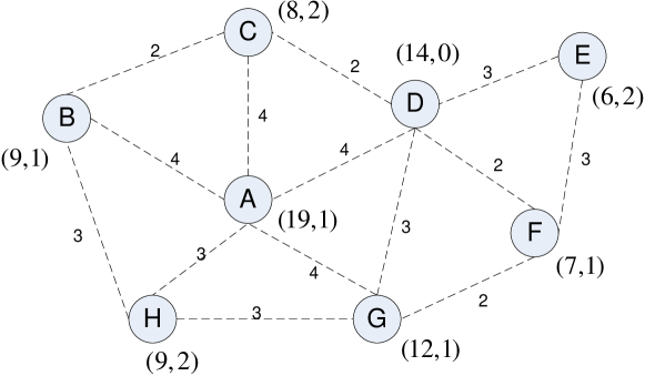
Figure 1: Connectivity graph of the example CRN and the connectivity vector $(d_{i},g_{i})$ for each node. The desired cluster size $\delta=3$. The sets of the indices of the available channels sensed by each node are: $K_{A}=\{1,2,3,4,5,6,10\},K_{B}=\{1,2,3,5,7\},K_{C}=\{1,3,4,10\},K_{D}=\{1,2,3,5\},K_{E}=\{2,3,5,7\},K_{F}=\{2,4,5,6,7\},K_{G}=\{1,2,3,4,8\},K_{H}=\{1,2,5,8\}$. Dashed edge indicates the end nodes are within each other’s transmission range.

4.1.1 Determining Cluster Heads and Forming Clusters

The procedure of determining the cluster heads is as follows. Each CR node decides whether it is a cluster head by comparing its connectivity vector with its neighbors. When CR node $i$ has lower individual connectivity degree than all its neighbors except for those which have already identified to be cluster heads, node $i$ becomes a cluster head. If there is another CR node $j$ in its neighborhood which has the same individual connectivity degree as $i$, i.e., $d_{j}=d_{i}$ and $d_{j}<d_{k},\forall k\in\text{Nb}(j)\setminus\{\Lambda\cup i\}$ where $\Lambda$ denotes the cluster heads, then the node between $i$ and $j$, which has higher neighborhood connectivity degree will become the cluster head, and the other node become one member of the newly identified cluster head. If $g_{i}=g_{j}$ as well, the node ID is used to break the tie, i.e., the one with smaller node ID becomes a cluster head. The node which is identified as a cluster head broadcasts a message to notify its neighbors of this change, and its neighbors which are not cluster heads become cluster members . The pseudo code for the cluster head decision and the initial cluster formation is shown in Algorithm 1 in the appendix.

After receiving the notification from a cluster head, a CR node $i$ is aware that it becomes a member of a cluster. Consequently, $i$ sets its individual connectivity degree to a positive number $M>|\mathcal{K}|\cdot N$, and broadcasts the new individual connectivity degree to all its neighbors. When a CR node $i$ is associated to multiple clusters, i.e., $i$ has received multiple notifications of cluster head eligibility from different CR nodes, $d_{i}$ is still set to be $M$. The manipulation of the individual connectivity degree of the cluster members fastens the speed of completing choosing the cluster heads. We have the following theorem to show that as long as a secondary user’s individual connectivity degree is greater than zero, every secondary user will eventually be either integrated into a certain cluster, or becomes a cluster head.

Theorem 4.1:

Given a CRN, it takes at most $N$ steps that every secondary user either becomes cluster head, or gets included into at least one cluster.

Here, by step we mean one secondary user executing Algorithm 4.1 for one time. The Proof is in Appendix 6.

The procedure of the proof also illustrates the time needed to conduct Algorithm 4.1. Consider an extreme scenario, where all the secondary nodes sequentially execute Algorithm 1, i.e., they constitute a list as discussed in the example in the proof. If one step can be finished within certain time $T$, then the total time needed for the network to conduct Algorithm 4.1 is $N*T$. In other scenarios, as Algorithm 1 can be executed concurrently by secondary users which locate in different places, the needed time can be considerably reduced. Let us apply Algorithm 1 to the example shown in Figure 1. Node $B$ and $H$ have the same individual connectivity degree, i.e., $d_{B}=d_{H}$. As $g_{H}=2>g_{B}=1$, node $H$ becomes the cluster head and cluster $C(H)$ is $\{H,B,A,G\}$.

4.1.2 Guarantee the Existence of Common Channels

After executing Algorithm 1, certain formed clusters may not possess any CCs. As decreasing cluster size increases the CCs within a cluster, for those clusters having no CCs, certain nodes need to be eliminated to obtain at least one CC. The sequence of elimination is performed according to an ascending list of nodes which are sorted by the number of common channels between the nodes and the cluster head. In other words, the cluster member which has the least common channels with the cluster head is excluded first. If there are multiple nodes having the same number of common channels with the cluster head, the node whose elimination brings in more common channels will be excluded. If this criterion meets a tie, the tie will be broken by deleting the node with smaller node ID. It is possible that the cluster head excludes all its neighbors and resulting in a singleton cluster which is composed by itself. The pseudo code for this procedure is shown in Algorithm 2. As to the nodes which are eliminated from the previous clusters, they restore their original individual connectivity degrees, execute Algorithm 1 and become either cluster heads or get included into other clusters afterwards according to Theorem 4.1.

During Phase I, when ever a CR node is decided to be a cluster head and accordingly forms a cluster, or its cluster’s composition is changed, the cluster head will broadcast the updated information about its cluster, which includes the sets of available channels on all its cluster members.

4.1.3 Cluster Size Control in Dense CRN

In this subsection, we illustrate the pressing necessity to control the cluster size when CRN becomes denser.

We consider a cluster $C(i)$ where $i$ is the cluster head in a dense CRN. To make the analysis easier, we assume there is no cluster heads which are generated within $i$’s neighborhood during the procedure of guaranteeing CCs. Assuming the CR users and PUs are evenly distributed and PUs occupy the licensed channels randomly, then both CR nodes density and channel availability in the CRN can be seen to be spatially homogeneous. In this case the formed clusters are decided by the transmission range and network density. According to Algorithm 1, the nearest cluster heads could locate just outside node $i$’s transmission range. An instance of this situation is shown in Figure 2. In the figure, black dots represent cluster heads, the circles denote the transmission ranges of cluster heads. Cluster members are not shown in the figure.

Figure 2: Clusters formation in extremely dense CRN. Black dots are cluster heads, cluster members are not drawn.

Let $l$ be the length of side of simulation plan square, and $r$ be CR’s transmission radius. Based on the aforementioned analysis and geometry illustration as shown in Figure 2, we give an estimate on the maximum number of generated clusters, which is the product of the number of cluster heads in one row and that number in one line, $l/r*l/r=l^{2}/r^{2}$. Given $r$=10 and $l$=50, the maximum number of clusters is 25. The number of clusters in the simulation is shown in Figure 3. Simulation is run for 50 times and the confidence interval is 95%. With the increase of CR users, network density (the average number of neighbours) increases linearly, and the number of clusters approaches to 25 which complies with the estimation.

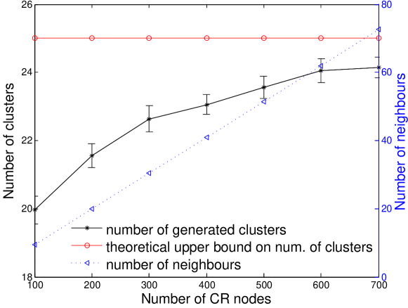
Figure 3: The correlation between the number of formed clusters and network density.

Both analysis and simulation show that when applying ROSS, after the clusters are saturated with the increase of network density, the cluster size increases linearly with the network density, thus certain measures are needed to curb this problem. This task falls to the cluster heads. To control the cluster size, cluster heads prune their cluster members to reach the desired cluster size. The desired size $\delta$ is decided based on the capability of the CR users and the tasks to be conveyed. As there are overlaps between neighboring clusters, the sizes of the clusters formed in this phase are larger than that of the finally formed clusters. Hence, a cluster head excludes some cluster members when the cluster size exceeds $t\cdot\delta$, where constant parameter $t$ is dependent on the network density and CR nodes’ transmission range and $t>1$. In particular, the cluster head removes the cluster members sequentially according to the following principle, the absence of one cluster member leads to the maximum increase of common channels within the cluster. This process ends when each cluster’s size is smaller or equal to $t\cdot\delta$. This procedure is similar with guaranteeing the existence of CCs in cluster, thus can reuse Algorithm 2. The $t$ is set to 1.3.

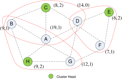
Figure 4: Clusters formation after the phase I of ROSS. CR nodes $A,B,D$ are debatable nodes as they belong to multiple clusters.

4.2 Phase II - Membership Clarification

As to the example CRN shown in Figure 1, the resulted clusters are shown in Figure 4 after running phase I of ROSS. We notice that nodes $A,B,D$ are included in more than one cluster. We refer to these nodes as debatable nodes as their cluster affiliations are not decided. The clusters which include the debatable node $i$ are called claiming clusters of node $i$, and the set of these clusters is denoted as $S_{i}$. The debatable nodes which are generated from the first phase of ROSS should be exclusively associated with only one cluster and be removed from the other claiming clusters, this procedure is called cluster membership clarification.

4.2.1 Distributed Greedy Algorithm (DGA)

Assume a debatable node $i$ needs to decide one cluster $C\in S_{i}$ to stay, and thereafter leaves the rest others in $S_{i}$. In this process, the principle for $i$ is that its move should result in the greatest increase of CCs in all its claiming clusters. Note that node $i$ is aware of the spectrum availability on all the cluster members of each claiming cluster, thus node $i$ is able to calculate how many more CCs can be produced in one claiming cluster if $i$ leaves that cluster. If there exists one cluster $C\in S_{i}$, when $i$ leaves this cluster brings the least increased CCs than leaving any other claiming clusters, then $i$ chooses to stay in cluster $C$. When there comes a tie, among the claiming clusters, $i$ chooses to stay in the cluster whose cluster head shares the most CCs with $i$. In case there are multiple claiming clusters demonstrating the same on the aforementioned metric, node $i$ chooses to stay in the claiming cluster which has the smallest size. Node IDs of cluster heads will be used to break tie if all the previous metrics could not decide on the unique claiming cluster for $i$ to stay. The pseudo code of this algorithm is given as Algorithm 3. After deciding its membership, debatable node $i$ notifies all its claiming clusters of its choice, and the claiming clusters from which node $i$ leaves also broadcast their new cluster composition and the spectrum availability on all their cluster members.

The autonomous decisions made by the debatable CR nodes raise the concern on the endless chain effect in the membership clarification phase. A debatable node’s choice is dependent on the compositions of its claiming clusters, which can be changed by other debatable nodes’ decisions. As a result, the debatable node which makes decision first may change its original choice, and this process may go on forever. To erase this concern, we formulate the process of membership clarification into a game, where a equilibrium is reached after a finite number of best response updates made by the debatable nodes.

4.2.2 Bridging ROSS-DGA with Congestion Game

Game theory is a powerful mathematical tool for studying, modelling and analysing the interactions among individuals. A game consists of three elements: a set of players, a selfish utility for each player, and a set of feasible strategy space for each player. In a game, the players are rational and intelligent decision makers, which are related with one explicit formalized incentive expression (the utility or cost). Game theory provides standard procedures to study its equilibriums [29]. In the past few years, game theory has been extensively applied to problems in communication and networking [30, 31]. Congestion game is an attractive game model which describes the problem where participants compete for limited resources in a non-cooperative manner, it has good property that Nash equilibrium can be achieved after finite steps of best response dynamic, i.e., each player choose strategy to maximizes/minimizes its utility/cost with respect to the other players’ strategies. Congestion game has been used to model certain problems in internet-centric applications or cloud computing, where self-interested clients compete for the centralized resources and meanwhile interact with each other. For example, server selection is involved in distributed computing platforms [32], or users downloading files from cloud, etc.

To formulate the debatable nodes’ membership clarification into the desired congestion game, we observe this process from a different (or opposite) perspective. From the new perspective, the debatable nodes are regarded to be isolated and don’t belong to any cluster, in other words, their claiming clusters become clusters which are beside them. Now for the debatable nodes, the previous problem of deciding which clusters to leave becomes a new problem that which cluster to join. In the new problem, debatable node $i$ chooses one cluster $C$ out of $S_{i}$ to join if the decrease of CCs in cluster $C$ is the smallest in $S_{i}$, and the decrease of CCs in cluster $C$ is $\sum_{C\in S_{i}}\Delta|K(C)|=\sum_{C\in S_{i}}({|K(C)|-|K(C\cup i)|})$. The interaction between the debatable nodes and the claiming clusters is shown in Figure 5.

Figure 5: Debatable nodes and claiming clusters

In the following, we show that the decision of debatable nodes to clarify their membership can be mapped to the behaviour of the players in a player-specific singleton congestion game when proper cost function is given. The game to be constructed is represented with a 4-tuple $\Gamma=(\mathcal{P},\mathcal{R},\sum_{i,i\in\mathcal{P}},f)$, and the elements in $\Gamma$ are explained below,

• $\mathcal{P}$, the set of players in the game, which are the debatable nodes in our problem.

• $\mathcal{R}=\cup S_{i},i\in\mathcal{P}$, denotes the set of resources for players to choose, in our problem, $S_{i}$ is the set of claiming clusters of node $i$, and $\mathcal{R}$ is the set of all claiming clusters.

• Strategy space $\sum_{i},i\in\mathcal{P}$ is the set of claiming clusters $S_{i}$. As debatable node $i$ is supposed to choose only one claiming cluster, then only one piece of resource will be allocated to $i$.

• The utility (cost) function $f(C)$ as to a resource $C$. $f(C)=\Delta|K^{i}(C)|,C\in S_{i}$, which represents the decreased number of CCs in cluster $C$ when debatable node $i$ joins $C$. As to cluster $C\in S_{i}$, the decrease of CCs caused by including the debatable nodes is $\sum_{i:C\in S_{i},i\rightarrow C}\Delta|K^{i}(C)|$. $i\rightarrow C$ means $i$ joins cluster $C$. Obviously this function is non-decreasing with respect to the number of nodes joining cluster $C$.

  The utility function $f$ is not purely decided by the number of players accessing the resource (debatable nodes join claiming clusters), which happens in a canonical congestion game. The reason is in this game the channel availability on debatable nodes is different. Given two same groups of debatable nodes and their sizes are the same, when the nodes are not completely the same (neither are the channel availabilities on these nodes), the cost happened on one claiming cluster could be different if the two groups of debatable nodes join that cluster respectively. Hence, this congestion game is player specific [33]. In this game, every player greedily updates its strategy (choosing one claiming cluster to join) if joining a different claiming cluster minimizes the decrease of CCs $\sum_{i:C\in S_{i}}\Delta|K^{i}(C)|$, and a player’s strategy in the game is exactly the same with the behaviour of a debatable node in the membership clarification phas.

As to singleton congestion game, there exists a pure equilibria which can be reached with the best response update, and the upper bound for the number of steps before convergence is $n^{2}*m$ [33], where $n$ is the number of players, and $m$ is the number of resources. In our problem, the players are the debatable nodes, and the resources are the claiming clusters. Thus the upper bound of the number of steps can be expressed as $\mathcal{O}(N^{3})$.

In fact, the number of steps which are actually involved in this process is much smaller than $N^{3}$, as both $n$ and $m$ are considerably smaller than $N$. The percentage of debatable nodes in $\mathcal{N}$ is illustrated in Figure 13, which is between 10% to 60% of the total number of CR nodes in the network. The number of clusters heads, as discussed in Section 4.1, is dependent on the network density and the CR node’s transmission range. As shown in Figure 3, the cluster heads take up only 3.4% to 20% of the total number of CR nodes.

4.2.3 Distributed Fast Algorithm (DFA)

On the basis of ROSS-DGA, we propose a faster version ROSS-DFA which differs from ROSS-DGA in the second phase. With ROSS-DFA, debatable nodes decide their respective cluster heads once. The debatable nodes consider their claiming clusters to include all their debatable nodes, thus the membership of claiming clusters is static and all the debatable nodes can make decision simultaneously without considering the change of membership of their claiming clusters. As ROSS-DFA is quicker than ROSS-DGA, the former is especially suitable for the CRN where the channel availability changes dynamically and re-clustering is necessary. To run ROSS-DFA, debatable node executes only one loop in Algorithm 3.

Now we apply both ROSS-DGA and ROSS-DFA to the toy network in Figure 4 which has been applied the phase I of ROSS. In the network, node $A$’s claiming clusters are cluster $C(C),C(H)\in S_{A}$, their members are $\{A,B,C,D\}$ and $\{A,B,H,G\}$ respectively. The two possible strategies of node $A$ is illustrated in Figure 6. In Figure 6(a), node $A$ staying in $C(C)$ and leaving $C(H)$ brings 2 more CCs to $S_{A}$, which is more than that brought by another strategy showed in 6(b). After the decisions made similarly by the other debatable nodes $B$ and $D$, the final clusters are formed as shown in Figure 7.

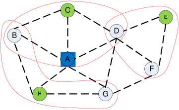
(a) Node A stays in cluster $C(C)$, quits $C(H)$, $\Delta|K(C(C))|+\Delta|K(C(H))|=2$

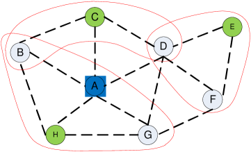
(b) Node A stays in cluster $C(H)$, quits $C(C)$, $\Delta|K(C(C))|+\Delta|K(C(H))|=1$

Figure 6: Membership clarification: possible cluster formations caused by node A’s different choices

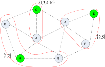
Figure 7: Final formation of clusters. Common channels are shown beside corresponding clusters.

5 Performance Evaluation

The schemes involved in the simulation are listed as follows,

• ROSS without size control, i.e., ROSS-DGA and ROSS-DFA.

• ROSS with size control. i.e., ROSS-$\delta$-DGA and ROSS-$\delta$-DFA where $\delta$ is the desired cluster size. In the following, we refer to the above mentioned four schemes as the variants of ROSS.

• SOC [21], a distributed clustering scheme pursuing cluster robustness.

• Centralized robust clustering scheme. The formulated optimization is an integer linear optimization problem, which is solved by MATLAB with the function $bintprog$.

The ROSS without size control mechanism is similar with the schemes proposed in [23]. The authors of [21] compared SOC with other schemes in terms of the average number of CCs of the formed cluster, on which SOC outperforms other schemes by 50%-100%. SOC’s comparison schemes are designed either for ad hoc network without consideration of channel availability [34], or for CRN but just considering connection among CR nodes [7]. Thus SOC is chosen to be the only distributed scheme as comparison, besides, we also compare ROSS with the centralized scheme.

Before we investigating the performance of the clustering schemes with simulation, we apply the two comparison clustering schemes in the example CRN in Figure 1, and make an initial comparison in terms of the amount of CCs. As to the centralized robust clustering scheme, we set the desired cluster size $\delta$ as 3, as a result, according to the network topology, the collection of all the possible clusters $\mathcal{S}=\{\{A\},\{B\},\dots,\{B,C\},\{B,A\},\{B,H\},\cdots,\{B,A,C\},$
$\{B,H,C\},\{A,D,C\},\cdots\}$, and $|\mathcal{S}|=38$. We set $\rho_{1}$ and $\rho_{1}$ as 0.2 and 0.8 respectively. The formed clusters by the centralized clustering scheme are shown in Fig. 8(b). The resulted clustering solutions from SOC is shown in Fig. 8(a). We compare the average number of CCs achieved by different schemes, the results of ROSS, centralized and SOC are 2.66, 2.66, and 3 respectively. Note there is one singleton cluster $C(H)$ generated by SOC, which is not preferred. When we only consider the clusters which are not singleton, the average number of CCs of SOC drops to 2.5.

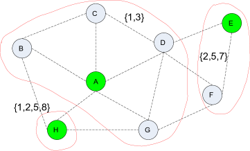
(a) Generated by SOC

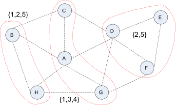
(b) Generated by the centralized clustering scheme

Figure 8: Final clusters formed by the centralized clustering scheme and SOC.

We investigate the schemes with four metrics.

• The average number of CCs per non-singleton cluster. Non-singleton cluster refers the cluster whose cluster size is larger than 1. Comparing with the metric adopted by SOC [21], which is the average number of CCs of all the clusters, this metric provides a more accurate description of the robustness of the non-singleton clusters. Having more CCs per non-singleton clusters means these clusters have longer life expectancy when the primary users’ operation becomes more intense. Although this metric doesn’t disclose the information about the unclustered CR nodes which are the synonyms of the singleton clusters, we still examine this metric as the number of CCs is involved in the utility adopted by all the variants of ROSS and SOC.

• Cluster sizes. We investigate the distribution of CRs residing in the formed clusters with different sizes.

• Robustness of the clusters against newly added PUs. We increase the number of PUs to challenge the non-singleton clusters, and count the number of the unclustered CR nodes. This metric directly indicates the robustness of clusters from a more practical point of view, i.e., as to the clusters formed for a given CRN and spectrum availability, how many CR nodes can still make use of the clusters when the spectrum availability decreases.

• Amount of control messages involved. We investigate the number of control messages involved in the clustering process.

Simulation consists of two parts, first we investigate the performance of centralized scheme and the distributed schemes in a small network, as there is no polynomial time solution available to solve the centralized problem. In the second part, we investigate the performance of the proposed distributed schemes in the CRN with different scales and densities. The following simulation settings is the same for both simulation parts. CRs and PUs are deployed on a two-dimensional Euclidean plane. The number of licensed channels is 10, each PU is operating on each channel with probability of 50%. CR users are assumed to be able to sense the existence of primary users and identify available channels. All primary and CR users are assumed to be static during the process of clustering. The simulation is written in C++, and the performance results are averaged over 50 randomly generated topologies, and the confidence interval corresponds to 95% confidence level.

5.1 Centralized Schemes vs. Decentralized Schemes

There are 10 primary users and 20 CR users dropped randomly (with uniform distribution) within a square area of size $A^{2}$, where we set the transmission ranges of primary and CR users to $A/3$. When clustering scheme is executed, around 7 channels are available on each CR node. The desired cluster size $\delta$ is 3. As to the centralized scheme, the parameters used in the punishment for choosing the clusters with undesired sizes are set as follows, $\rho_{1}=0.4$, $\rho_{2}=0.6$.

5.1.1 Average number of CCs in Non-singleton Clusters

From Figure 12, we can see the centralized schemes outperform the distributed schemes. Among the distributed schemes, SOC achieves the most CCs. The reason is, SOC is liable to group the neighboring CRs which share the most abundant spectrum together, no matter how many of them are there, thus the number of CC of the formed clusters is higher. In the other hand, SOC generates the most unclustered CRs, which can be seen when we discuss the performance on the number of unclustered CR nodes. As to the variants of ROSS, we notice that the greedy mechanism increases CCs in non-singleton clusters significantly.

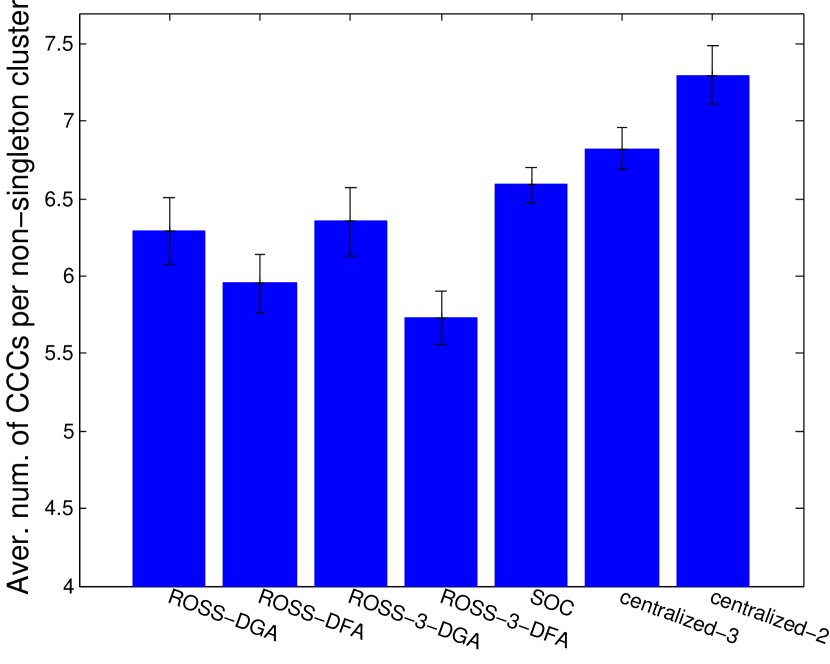
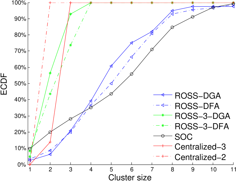
Figure 9: Number of common channels of non-singleton clusters

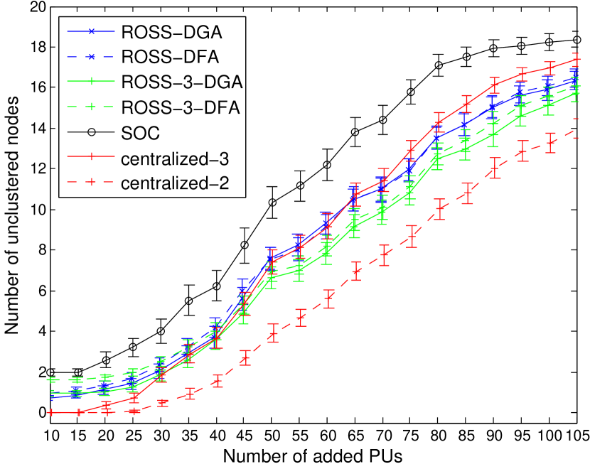
Figure 10: Cumulative distribution of CRs residing in clusters with different sizes

Figure 11: Number of unclustered CRs with decreasing spectrum availability

Figure 12: Comparison between the distributed and centralized clustering schemes ($N$ = 20)

5.1.2 Cluster Size

Figure 12 depicts the empirical cumulative distribution of the CRs in clusters of different sizes, from which we have two conclusions. The first, SOC generates more unclustered CR nodes than other schemes. The centralized schemes don’t produce unclustered CR nodes in the simulation, the unclustered nodes generated by ROSS-DGA/DFA account for 3% of the total CR nodes, as comparison, 10% of nodes are unclustered when applying SOC. ROSS-DGA and ROSS-DFA with size control feature generate 5%-8% unclustered CR nodes, which is due to the cluster pruning procedure (discussed in section 4.1.2 and section 4.1.3). Second, the centralized schemes and cluster size control mechanism of ROSS generate clusters with the desired cluster size. As to ROSS-DFG and ROSS-DFA with size control feature, CR nodes reside averagely in clusters whose sizes are 2, 3 and 4. The sizes of clusters resulted from ROSS-DGA and ROSS-DFA are disperse, but appear to be better than SOC, i.e., the 50% percentiles for ROSS-DGA, ROSS-DFA and SOC are 4.5, 5, and 5.5, and the 90% percentiles for the three schemes are 8, 8, and 9, the corresponding sizes of ROSS are closer to the desired size.

5.1.3 Robustness of the clusters against newly added PUs

In this part of simulation, we put PUs sequentially into CRN to decrease the available spectrum. 10 PUs are in the network in the beginning, then extra 19 batches of PUs are added sequentially, where each batch includes 5 PUs.

Figure 12 shows certain clusters can not maintain and the number of unclustered CR nodes grows when the number of PUs increases. The centralized scheme with desired size of 2 generates the most robust clusters, meanwhile, SOC results in the most vulnerable clusters. The centralized scheme with desired size of 3 doesn’t outperform the variants of ROSS, because pursuing cluster size prevents forming the the clusters with more CCs. In contrary, the variants of ROSS generate some smaller clusters which are more likely to maintain when there are more PUs.

5.1.4 Control Signaling Overhead

In this section we compare the overhead of signaling involved in different clustering schemes. We don’t consider the the control messages which are involved in neighborhood discovery, which is the premise and deemed to be the same for all clustering schemes. According to [35], the message complexity is defined as the number of messages used by all nodes. To have the same metric to compare, we count the number of transmissions of control messages, without distinguishing broadcast or uni-cast control messages. This metric is synonymous with the number of updates discussed in Section 4.

As to ROSS, the control messages are generated in both phases. In the first phase, when a CR node decides itself to be the cluster head, it broadcasts a message containing its ID, cluster members and the set of CCs in its cluster. In the second phase, a debatable node broadcasts its affiliation to inform its claiming clusters, then the cluster heads of the claiming clusters broadcast message about the new cluster members if they are changed due to the debatable node’s decision. The upper bound of the total number of the control messages involved in cluster formation is analyzed in Theorem 4.1 and Section 4.2.2.

The comparison scheme SOC involves three rounds of execution. In the first two rounds, every CR node maintains its own cluster and seeks either to integrate neighboring clusters or to join one neighboring cluster. The final clusters are obtained in the third round. In each round, every CR node is involved in comparisons and cluster mergers.

The centralized scheme is conducted at the centralized control device, but it involves two phases of control message transmission. The first phase is information aggregation, in which every CR node’s channel availability and neighborhood is transmitted to the centralized controller. iIn the second phase, the control broadcasts the clustering solution, which is disseminated to every CR node. We adopt the algorithm proposed in [36] to broadcast and gather information as the algorithm is simple and self-stabilizing. This scheme needs building a backbone structure to support the communication. We apply ROSS to generate cluster heads which serve as the backbone, and the debatable nodes are used as the gateway nodes between the backbone nodes. As the backbone is built for one time and supports the transmission of control messages later on, we don’t take account the messages involved in building the backbone. As to the process of information gathering, we assume that every cluster member sends the spectrum availability and its ID to its cluster head, which further forwards the message to the controller, then the number of transmissions is $N$. As to the process of dissemination, in an extreme situation where all the gateway and the backbone nodes broadcast, the number of transmissions is $h+m$, where $h$ is the number of cluster heads and $m$ is number of debatable nodes.

The number of control messages which are involved in ROSS variants and the centralized scheme is related with the number of debatable nodes. Figure 13 shows the percentage of debatable nodes with different network densities, from which we can obtain the value of $m$.

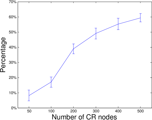
Figure 13: The percentage of debatable nodes after phase I of ROSS.

Table 5.1.4 shows the message complexity, quantitative amount of the control messages, and the size of control messages. Figure 14 shows the analytical result of the amount of transmissions involved in different schemes.

Table II: Signalling overhead

Scheme	Message Complexity	Quantitative number of messages	Content of message (size of message)
ROSS-DGA, ROSS-$\delta$-DGA	$\mathcal{O}(N^{3})$ (worst case)	$h+2m^{2}d$ (upper bound)	Cluster head $i$ broadcasts channel availability on all cluster members ($|C(i)||\mathcal{K}|$ bytes); Cluster member $i$ broadcasts the new individual connectivity $d_{i}$ after being included in one or more clusters (1 byte)
ROSS-DFA, ROSS-$\delta$-DFA	$\mathcal{O}(N)$ (worst case)	$h+2m$ (upper bound)
SOC	$\mathcal{O}(N)$	$3N$	Every CR node $i$ broadcasts channel availability on all cluster members ($|C(i)||\mathcal{K}|$ bytes)
Centralized	$\mathcal{O}(N)$	$h+m+N$ (upper bound) [36]	clustering result (2$N$ bytes) tnote:robots-r1

1. Assuming the data structure of the clustering result is in the form of { Node ID $i$, cluster head ID h($C$) where $i\in C$, for every $i\in\mathcal{N}$ }.

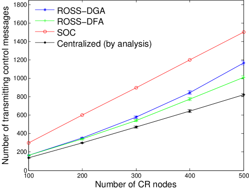
Figure 14: Quantitative amount of control messages.

5.2 Comparison among the Distributed Schemes

In this section we investigate the performances of distributed clustering schemes in CRN with different network scales and densities. The transmission range of CR is $A/5$, PU’s transmission range is $2A/5$. The initial number of PU is 30. The desired sizes adopted are listed in the Table III, which is about 60% of the average number of neighbours. When run ROSS, the parameter $t$ which is used to control cluster size in phase I is 1.3.

Table III:

Number of CRs	100	200	300
Average num. of neighbours	9.5	20	31
Desired size $\delta$	6	12	20

5.2.1 Number of CCs per Non-singleton Clusters

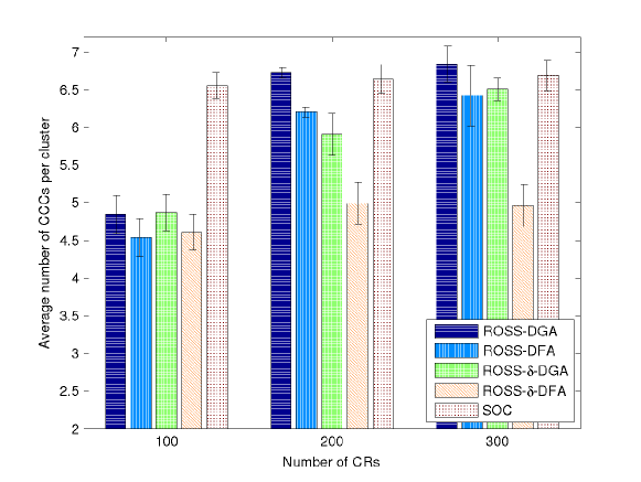
Figure 15: Number of common channels of non-singleton clusters.

Figure 15 shows the average number of CCs of the non-singleton clusters. We notice that SOC achieves the most CCs per non-singleton cluster, although the lead over the variants of ROSS shrinks significantly when $N$ increases.

5.2.2 Robustness of the clusters against newly added PUs

We add extra 20 batches of PUs sequentially in the CRN, where each batch includes 10 PUs. Figure 19 and 19 show that when $N=100$ and 200, more unclustered CR nodes appear in the CRN where SOC is applied. When the network becomes denser, as shown in Figure 19, ROSS-DGA/DFA generate slightly more unclustered CR nodes than SOC when new PUs are not many, but SOC’s performance deteriorates quickly when the number of PUs becomes larger. We only show the average values of the variants of ROSS as their confidence intervals overlap. When applying ROSS with size control mechanism, significantly less unclustered CR nodes are generated. Besides, the greedy mechanism moderately strengthens the robustness of the clusters.

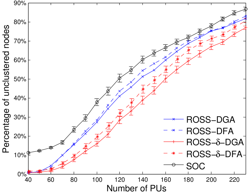
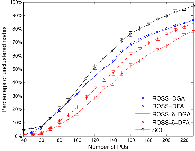
Figure 16: 100 CRs

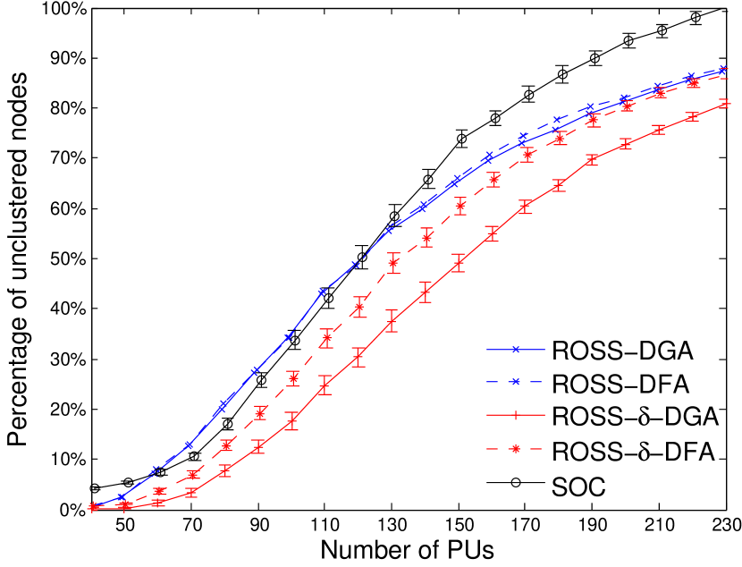
Figure 17: 200 CRs

Figure 18: 300 CRs

Figure 19: Percentage of CR nodes which are not included in any non-singleton clusters

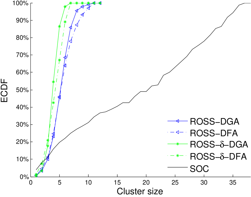
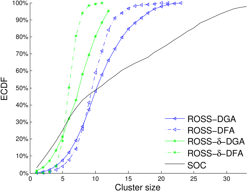
Figure 20: 100 CRs, 30 PUs in network

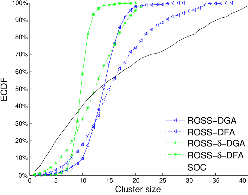
Figure 21: 200 CRs, 30 PUs in network

Figure 22: 300 CRs, 30 PUs in network

Figure 23: Cumulative distribution of CRs residing in clusters with different sizes

5.2.3 Cluster Size Control

Figure 24 shows when the network density scales up, the number of formed clusters by ROSS increases by smaller margin, and that generated by SOC increases linearly. This result coincides with the analysis in Section 4.1.3. To better understand the distribution of the sizes of formed clusters, we depict the empirical cumulative distribution of CR nodes in clusters with different sizes in Figures 23 23 23.

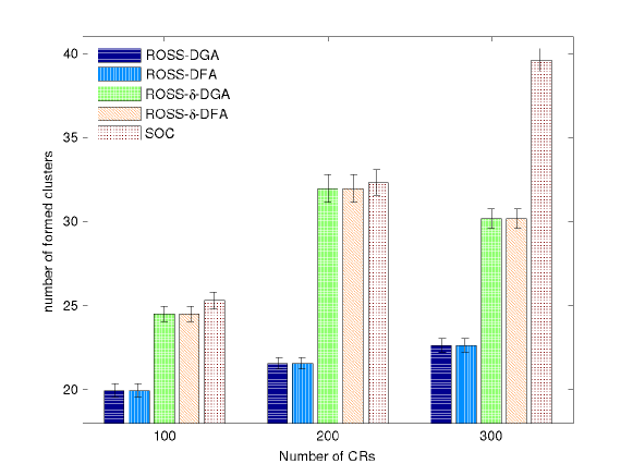
Figure 24: The number of formed clusters.

The sizes of clusters generated by ROSS-DGA and ROSS-DFA span a wider range than ROSS with size control feature. Most of the generated clusters are smaller than the average number of neighbours, which is roughly equal with the 95% percentile of the ROSS-DGA curve. The 50% percentile of the ROSS-DGA curve is roughly the desired size $\delta$. When the variants of ROSS with size control feature are applied, the sizes of the most generated clusters are smaller than $\delta$. As to the curves of SOC, the 95% percentiles are 36, 30, and 40 in respective networks. From Figure 23, we conclude that the sizes of the clusters generated by ROSS are limited by the network density, the sizes of the clusters formed by ROSS with size control feature are restricted by the desired size. In contrary, the clusters generated from SOC demonstrate strong divergence on cluster sizes.

5.3 Insights Obtained from the Simulation

The centralized clustering scheme is able to form the clusters which satisfy the requirement on cluster size strictly, and the clusters are robust against the PUs’ activity, besides, it generates the smallest control overhead in the process of clustering.

As distributed schemes, the variants of ROSS outperform SOC considerably on three metrics. The variants of ROSS generate much less singleton clusters than SOC, and the resulted clusters are robuster than SOC when facing the newly added PUs. The signaling overhead involved in ROSS is about half of that needed for SOC, and the signaling messages are much shorter that the latter. The sizes of the clusters generated by ROSS demonstrate smaller discrepancy than that of SOC. Besides, the ROSS variants with size control features achieve similar performance to the centralized scheme in terms of cluster size, and the cluster robustness is similar when applying the variants of ROSS and the centralized scheme respectively.

As to the variants of ROSS, the greedy mechanism in ROSS-DGA helps to improve the performance on cluster size and cluster robustness at the cost of mildly increased signaling overhead. We also notice that as a metric, the number of CCs per non-singleton cluster doesn’t indicate the robustness of clusters as shown in Figure 12 and 19, although it is adopted as the metric in the formation of clusters.

6 Conclusion

In this paper we investigate the robust clustering problem in CRN extensively. We provide the mathematical description of the problem and prove the NP hardness of it. We propose both centralized and distributed schemes ROSS, the cluster structure generated by them has longer time expectancy against the primary users’ activity. Besides, the proposed schemes can generate clusters with desired sizes. The congestion game model in game theory is used to design the distributed schemes. Through simulation and theoretical analysis, we find that distributed schemes achieve similar performance with centralized optimization in terms of cluster robustness, signaling overhead and cluster sizes, and outperform the comparison distributed scheme on the above mentioned metrics.

The shortcoming of distributed scheme ROSS is it doesn’t generate clusters whose sizes exceed the cluster head’s neighborhood. The reason is with ROSS, cluster heads form clusters on the basis of their neighborhood, and don’t involve the nodes which are outside the neighborhood. In the other way around, forming big cluster which extends a cluster head’s neighborhood has limited application scenarios, as multiple hop communication and coordination are required within these clusters.

Input: $d_{j},g_{j},j\in\text{Nb}_{i}\setminus\Lambda$, $\Lambda$ means cluster heads. Empty sets $\tau_{1},\tau_{2}$

Result: Returning 1 means $i$ is cluster head, then $d_{j}$ is set to 0, $j\in\text{Nb}_{i}\setminus\Lambda$. returning 0 means $i$ is not cluster head.

1

2if $\nexists j\in\text{Nb}_{i}\setminus\Lambda$, such that $d_{i}\geq d_{j}$ then

3       return 1;

4 end if

5if $\exists j\in\text{Nb}_{i}\setminus\Lambda$, such that $d_{i}>d_{j}$ then

6       return 0;

7else

8       if $\nexists j\in\text{Nb}_{i}\setminus\Lambda$, such that $d_{j}==d_{i}$ then

9             $\tau_{1}\leftarrow j$

10       end if

11      

12 end if

13if $\nexists j\in\tau_{1}$, such that $g_{i}\leq g_{j}$ then

14       return 1;

15 end if

16if $\exists j\in\tau_{1}$, such that $g_{i}<g_{j}$ then

17       return 0;

18else

19      if $\nexists j\in\tau_{1}$, such that $g_{j}==g_{i}$ then

20             $\tau_{2}\leftarrow j$

21       end if

22      

23 end if

24if $\texttt{ID}_{i}$ is smaller than any $\texttt{ID}_{j}$, $j\in\tau_{2}\setminus i$ then

25       return 1;

26 end if

return 0;

Algorithm 1 ROSS phase I: cluster head determination and initial cluster formation for CR node $i$

Input: Cluster C, empty sets $\tau_{1},\tau_{2}$

Output: Cluster C has at least one CC, or satisfies the requirement on cluster size

1 while $K_{C}=\emptyset$ do

2       while $|C|>t\cdot\delta$ do

3             if $\exists$ only one $i\in C\setminus H_{C}$, $i=\operatorname*{arg\,min}(|K_{H_{C}}\cap K_{i}|)$ then

4                   $C=C\setminus i$;

5            else

6                   $\exists$ multiple $i$ which satisfies $i=\operatorname*{arg\,min}(|K_{H_{C}}\cap K_{i}|)$;

7                   $\tau_{1}\leftarrow i$;

8             end if

9            

10            if $\exists$ only one $i\in\tau_{1}$, $i=\operatorname*{arg\,max}(|\cap_{j\in C\setminus i}K_{j}|-|\cap_{j\in C}K_{j}|)$ then

11                   $C=C\setminus i$;

12            else

13                   $C=C\setminus i$, where $i=\operatorname*{arg\,min}_{i\in\tau_{1}}\texttt{ID}_{i}$

14             end if

15            

16       end while

17      

18 end while

Algorithm 2 ROSS phase I: cluster head guarantees the availability of CC (start from line 1) / cluster size control (start from line 2)

Input: all claiming clusters $C\in S_{i}$

Output: one cluster $C\in S_{i}$, node $i$ notifies all its claiming clusters in $S_{i}$ about its affiliation decision.

1 while $i$ has not chosen the cluster, or $i$ has joined cluster $\tilde{C}$, but $\exists C^{\prime}\in S_{i},C^{\prime}\neq\tilde{C}$, which has $|K(C^{\prime}\setminus i)|-|K(C^{\prime})|<|K(C\setminus i)|-|K(C)|$ do

2       if $\exists$ only one $C\in S_{i}$, $C=\operatorname*{arg\,min}(|K(C\setminus i)|-|K(C)|)$ then

3             return $C$;

4      else

5             $\exists$ multiple $C\in S_{i}$ which satisfies $C=\operatorname*{arg\,min}(|K(C\setminus i)|-|K(C)|)$;

6             $\tau_{1}\leftarrow C$;

7       end if

8      if $\exists$ only one $C\in\tau_{1}$, $C=\operatorname*{arg\,max}(K_{h_{C}}\cap K_{i})$ then

9             return $C$;

10      else

11             $\exists$ multiple $C\in S_{i}$ which satisfies $C=\operatorname*{arg\,max}(K_{h_{C}}\cap K_{i})$;

12             $\tau_{2}\leftarrow C$;

13       end if

14      if $\exists$ only one $C\in\tau_{2}$, $C=\operatorname*{arg\,min}|C|)$ then

15             return $C$;

16      else

17             return $\operatorname*{arg\,min}_{C\in\tau_{2}}h_{C}$;

18            

19       end if

20      

21 end while

Algorithm 3 Debatable node $i$ decides its affiliation in phase II of ROSS

Proof of Theorem 4.1

• We consider a CRN which can be represented as a connected graph. To simplify the discussion, we assume the secondary users have unique individual connectivity degrees. Each user has an identical ID and a neighborhood connectivity degree. This assumption is fair as the neighborhood connectivity degrees and node ID are used to break ties in Algorithm 1, when the individual connectivity degrees are unique, it is not necessary to use the former two metrics.

  For the sake of contradiction, let us assume there exist some secondary user $\alpha$ which is not included into any cluster. Then there is at least one node $\beta\in\text{Nb}_{\alpha}$ such that $d_{\alpha}>d_{\beta}$. According to Algorithm 1, $\delta$ is not included in any clusters, because otherwise $d_{\beta}=M$, a large positive integer. Now, we distinguish between two cases: If $\beta$ becomes cluster head, node $\alpha$ is included, the assumption is not true. If $\beta$ is not a cluster head, then $\beta$ is not in any cluster, we can repeat the previous analysis made on node $\alpha$, and deduce that node $\beta$ has at least one neighbouring node $\gamma$ with $d_{\gamma}<d_{\beta}$. Till now, when there is no cluster head identified, the unclustered nodes, i.e., $\alpha$, $\beta$ form a linked list, where their connectivity degrees monotonically decrease. But this list will not continue to grow, because the minimum individual connectivity degree is zero, and the length of this list is upper bounded by the total number of nodes in the CRN. An example of the formed node series is shown as Figure 25.

  

  Figure 25: The node series discussed in the proof of Theorem 4.1, the deduction begins from node $\alpha$

In this example, node $\omega$ is at the tail of the list. As $\omega$ does not have neighboring nodes with lower individual connectivity degree, $\omega$ becomes a cluster head. Then $\omega$ incorporates all its one-hop neighbours (here we assume that every newly formed cluster has common channels), including the nodes which precede $\omega$ in the list. The nodes which join a cluster set their individual connection degrees to $M$, which enables the node immediately precede in the list to become a cluster head. In this way, cluster heads are generated from the tail of list to the head of the list, and all the nodes in the list are in at least one cluster, which contradicts the assumption that $\alpha$ is not included in any cluster.

If we see a secondary user becoming a cluster head, or becoming a cluster member as one step, as the length of the list of secondary users is not larger than $N$, there are $N$ steps for this scenario to form the initial clusters.

∎

Proof of Theorem 3.1

• To prove the robust clustering problem is NP-hard, we reduce the maximum weighted k-set packing problem, which is NP-hard when $k\geqslant 3$ [37], to the the robust clustering problem to show the latter is at least as hard as the former. Given a collection of sets of cardinality at most $k$ with weights for each set, the maximum weighted packing problem is that of finding a collection of disjoint sets of maximum total weight. The decision version of weighted $k$-set packing problem is,

  Definition 2:

  Given a finite set $\mathcal{G}$ of non-negative integers where $\mathcal{G}\subsetneq\mathbb{N}$, and a collection of sets $\mathcal{Q}=\{S_{1},S_{2},\cdots,S_{m}\}$ where $S_{i}\subseteq\mathcal{G}$ and $\max(S_{i})\geq 3$ for $1\leq i\leq m$. Every set $S$ in $\mathcal{Q}$ has a weight $\omega(S)\in\mathbb{R}$. The problem is to find a collection $\mathcal{S}\subseteq\mathcal{Q}$ such that $\mathcal{S}$ contains only pairwise disjoint sets and the total weight of the sets in $\mathcal{S}$ is greater than a given positive number $\lambda$, i.e., $\sum_{S\in\mathcal{S}}\omega(S)>\lambda$.

We assume the weights of sets are positive integers. Then we will show that any instance $\mathcal{I}$ of a weighted $k$-set packing problem, i.e., a collection of sets, can be transformed to a clusters formation for a CRN. W.l.o.g. let set $\mathcal{G}=\{1,\ldots,N\}$. The polynomial algorithm $\sigma$ consists of three steps.

• First, the sets in the instance $\mathcal{I}$ are mapped sequentially to the clusters of CR nodes on a two-dimensional Euclidean plane, where the CR user ID is identical with the corresponding element’s index.

• Second, for each mapped cluster $C$, we assign the channels for the nodes in $C$ so that $|K(C)|$ equals to the $\omega(S)$. We can simply assign the first $|K(C)|$ channels to each CR node in $C$, without considering the possible mismatch when the same CR node appears in different clusters and is assigned with different channels.

The number of steps is dependent on $\mathcal{I}$, which is between 1 and $N^{2}$

Assume we have a robust clustering black box which can check whether the clustering instance meets the requirement, i.e., clusters are not overlapping and the total sum of CCs exceed $\lambda$ or not. If yes is said, then the total weight of the corresponding instance of the maximum weighted k-set packing problem is greater than $\lambda$. If the black box said no, either due to overlapping clusters, or the sum of CCs over all clusters is smaller than $\lambda$, the corresponding instance of the packing problem is not an solution.

Hence, the weighted $k$-set packing can be reduced to the robust clustering problem in CRN, then the latter problem is of NP-hard.

∎

References

- [1] J. Mitola and G. Q. Maguire, “Cognitive radio: making software radios more personal,” IEEE Personal Communications, vol. 6, no. 4, pp. 13–18, Aug 1999.
- [2] T. Yucek and H. Arslan, “A survey of spectrum sensing algorithms for cognitive radio applications,” IEEE Communications Surveys Tutorials, vol. 11, no. 1, pp. 116–130, First 2009.
- [3] Q. Zhao and B. Sadler, “A survey of dynamic spectrum access,” Signal Processing Magazine, IEEE, vol. 24, no. 3, pp. 79–89, May 2007.
- [4] A. Sahai, R. Tandra, S. M. Mishra, and N. Hoven, “Fundamental design tradeoffs in cognitive radio systems,” in Proc. of ACM TAPAS ’06.
- [5] I. F. Akyildiz, B. F. Lo, and R. Balakrishnan, “Cooperative spectrum sensing in cognitive radio networks: A survey,” Phys. Commun., vol. 4, no. 1, pp. 40–62, Mar. 2011.
- [6] C. Sun, W. Zhang, and K. B. Letaief, “Cluster-based cooperative spectrum sensing in cognitive radio systems,” in proc. of IEEE ICC 2007.
- [7] J. Zhao, H. Zheng, and G.-H. Yang, “Spectrum sharing through distributed coordination in dynamic spectrum access networks,” Wireless Com. and Mobile Computing, vol. 7, no. 9, 2007.
- [8] D. Willkomm, M. Bohge, D. Hollós, J. Gross, and A. Wolisz, “Double hopping: A new approach for dynamic frequency hopping in cognitive radio networks,” in Proc. of PIMRC 2008.
- [9] C. Passiatore and P. Camarda, “A centralized inter-network resource sharing (CIRS) scheme in IEEE 802.22 cognitive networks,” in Proc. of IFIP Annual Mediterranean Ad Hoc Networking Workshop 2011.
- [10] A. A. Abbasi and M. Younis, “A survey on clustering algorithms for wireless sensor networks,” Comput. Commun., vol. 30, no. 14-15, pp. 2826–2841, 2007.
- [11] Q. Wu, G. Ding, J. Wang, X. Li, and Y. Huang, “Consensus-based decentralized clustering for cooperative spectrum sensing in cognitive radio networks,” Chinese Science Bulletin, vol. 57, 2012.
- [12] H. D. R. Y. Huazi Zhang, Zhaoyang Zhang1 and X. Chen, “Distributed spectrum-aware clustering in cognitive radio sensor networks,” in Proc. of GLOBECOM 2011.
- [13] B. E. Ali Jorio, Sanaa El Fkihi and D. Aboutajdine, “An energy-efficient clustering routing algorithm based on geographic position and residual energy for wireless sensor network,” Journal of Computer Networks and Communications, vol. 2015, 04 ’15.
- [14] V. Kawadia and P. R. Kumar, “Power control and clustering in ad hoc networks,” in Proc. of INFOCOM ’03, 2003, pp. 459–469.
- [15] M. Krebs, A. Stein, and M. A. Lora, “Topology stability-based clustering for wireless mesh networks,” in IEEE GLOBECOM 2010.
- [16] T. Chen, H. Zhang, G. Maggio, and I. Chlamtac, “Cogmesh: A cluster-based cognitive radio network,” Proc. of DySPAN ’07.
- [17] K. Baddour, O. Ureten, and T. Willink, “Efficient clustering of cognitive radio networks using affinity propagation,” in Proc. of ICCCN 2009.
- [18] D. Wu, Y. Cai, L. Zhou, and J. Wang, “A cooperative communication scheme based on coalition formation game in clustered wireless sensor networks,” IEEE Transactions on Wireless Communications,, vol. 11, no. 3, pp. 1190 –1200, march 2012.
- [19] A. Asterjadhi, N. Baldo, and M. Zorzi, “A cluster formation protocol for cognitive radio ad hoc networks,” in Proc. of European Wireless Conference 2010, pp. 955–961.
- [20] M. Ozger and O. B. Akan, “Event-driven spectrum-aware clustering in cognitive radio sensor networks,” in Proc. of IEEE INFOCOM 2013.
- [21] S. Liu, L. Lazos, and M. Krunz, “Cluster-based control channel allocation in opportunistic cognitive radio networks,” IEEE Trans. Mob. Comput., vol. 11, no. 10, pp. 1436–1449, 2012.
- [22] N. Mansoor, A. Islam, M. Zareei, S. Baharun, and S. Komaki, “Construction of a robust clustering algorithm for cognitive radio ad-hoc network,” in Proc. of CROWNCOM 2015.
- [23] D. Li and J. Gross, “Robust clustering of ad-hoc cognitive radio networks under opportunistic spectrum access,” in Proc. of IEEE ICC ’11.
- [24] B. Clark, C. Colbourn, and D. Johnson, “Unit disk graphs,” Annals of Discrete Mathematics, vol. 48, no. C, pp. 165–177, 1991.
- [25] Y. Zhang, G. Yu, Q. Li, H. Wang, X. Zhu, and B. Wang, “Channel-hopping-based communication rendezvous in cognitive radio networks,” IEEE/ACM Transactions on Networking, vol. 22, no. 3, pp. 889–902, June 2014.
- [26] Z. Gu, Q.-S. Hua, and W. Dai, “Fully distributed algorithms for blind rendezvous in cognitive radio networks,” in Proceedings of the 2014 ACM MobiHoc, ser. MobiHoc ’14.
- [27] Y. P. Chen, A. L. Liestman, and J. Liu, “Clustering algorithms for ad hoc wireless networks,” in Ad Hoc and Sensor Networks. Nova Science Publishers, 2004.
- [28] E. Perevalov, R. S. Blum, and D. Safi, “Capacity of clustered ad hoc networks: how large is "large"?” IEEE Transactions on Communications, vol. 54, no. 9, pp. 1672–1681, Sept 2006.
- [29] A. MacKenzie and S. Wicker, “Game theory in communications: motivation, explanation, and application to power control,” in Proc. of IEEE GLOBECOM 2001.
- [30] J. O. Neel, “Analysis and design of cognitive radio networks and distributed radio resource management algorithms,” Ph.D. dissertation, Blacksburg, VA, USA, 2006, aAI3249450.
- [31] B. Wang, Y. Wu, and K. R. Liu, “Game theory for cognitive radio networks: An overview,” Comput. Netw., vol. 54, no. 14, pp. 2537–2561, Oct. 2010.
- [32] B. J. S. Chee and C. Franklin, Jr., Cloud Computing: Technologies and Strategies of the Ubiquitous Data Center, 1st ed. CRC Press, Inc., 2010.
- [33] H. Ackermann, H. Röglin, and B. Vöcking, “Pure Nash equilibria in player-specific and weighted congestion games,” Theoretical Computer Science, vol. Vol. 410, no. 17, pp. 1552 – 1563, 2009.
- [34] S. Basagni, “Distributed clustering for ad hoc networks,” Proc. of I-SPAN ’99, pp. 310 –315, 1999.
- [35] X.-Y. Li, Y. Wang, and Y. Wang, “Complexity of data collection, aggregation, and selection for wireless sensor networks,” IEEE Transactions on Computers, vol. 60, no. 3, pp. 386–399, 2011.
- [36] M. Onus, A. Richa, K. Kothapalli, and C. Scheideler, “Efficient broadcasting and gathering in wireless ad-hoc networks,” in Proc. of ISPAN 2005.
- [37] M. R. Garey and D. S. Johnson, Computers and Intractability: A Guide to the Theory of NP-Completeness. W. H. Freeman, 1979.