Stability Analysis of Einstein Universe in $f(\mathcal{G},T)$ Gravity

Abstract

This paper explores stability of the Einstein universe against linear homogeneous perturbations in the background of $f(\mathcal{G},T)$ gravity. We construct static as well as perturbed field equations and investigate stability regions for the specific forms of generic function $f(\mathcal{G},T)$ corresponding to conserved as well as non-conserved energy-momentum tensor. We use the equation of state parameter to parameterize the stability regions. The graphical analysis shows that the suitable choice of parameters lead to stable regions of the Einstein universe.

Keywords: Stability analysis; Einstein universe; $f(\mathcal{G},T)$ gravity.
PACS: 04.25.Nx; 04.40.Dg; 04.50.Kd.

1 Introduction

The current accelerated expansion of the universe is one of the most astonishing discovery in golden era of cosmology. This has stimulated many researchers to explore the enigmatic nature of dark energy (DE) which is responsible for the phase of cosmic accelerated expansion. Dark energy possesses large negative pressure with repulsive nature but its many salient features are still not known. Modified theories of gravity are considered as the most favorable and optimistic approaches among other proposals to explore the nature of DE. These theories are established by replacing or adding curvature invariants and their corresponding generic functions in the geometric part of general relativity (GR).

The Einstein field equations are derived from the first Lovelock scalar dubbed as the Ricci scalar $(R)$ in the Lagrangian density which corresponds to gravity while a particular form of quadratic curvature invariants yields second Lovelock scalar known as Gauss-Bonnet (GB) invariant. This invariant is a linear combination of the form $\mathcal{G}=R^{2}-4R_{\mu\nu}R^{\mu\nu}+R_{\mu\nu\alpha\beta}R^{\mu\nu\alpha\beta}$, where $R_{\mu\nu}$ and $R_{\mu\nu\alpha\beta}$ represent the Ricci and Riemann tensors, respectively. Gauss-Bonnet invariant is four-dimensional $(4D)$ topological term which has the feature like it is free from spin-2 ghost instabilities [1]. There are two interesting approaches to discuss the dynamics of $\mathcal{G}$ in $4D$ either by coupling with scalar field or by adding the generic function $f(\mathcal{G})$ in the Einstein-Hilbert action. The first approach naturally appears in the effective low energy action in string theory which effectively discusses the singularity-free cosmological solutions [2].

Nojiri and Odintsov [3] introduced second approach as an alternative for DE known as $f(\mathcal{G})$ gravity which elegantly studies the fascinating characteristics of late-time cosmology. Cognola et al. [4] investigated DE cosmology and found that this theory effectively describes the cosmological structure with a possibility to describe the transition from decelerated to accelerated cosmic phases. De Felice and Tsujikawa [5] constructed some cosmological viable $f(\mathcal{G})$ models and introduced a procedure to avoid numerical instabilities related with a large mass of the oscillating mode. The same authors [6] also found that the solar system constraints are consistent for a wide range of cosmological viable model parameters.

The captivating issue of cosmic accelerated expansion has successfully been discussed by taking into account modified theories of gravity with matter-curvature coupling. Harko et al. [7] presented $f(R,T)$ gravity ($T$ is the trace of energy-momentum tensor (EMT)) to study the coupling between geometry and matter. Recently, we introduced another modified theory named as $f(\mathcal{G},T)$ gravity which is a generalization of $f(\mathcal{G})$ gravity [8]. This modification is based on the coupling of quadratic curvature invariant with matter just as $f(R,T)$ gravity. We studied the non-zero covariant divergence of EMT due to matter-curvature coupling and the massive test particles followed non-geodesic trajectories due to the presence of extra force while the dust particles moved along geodesic lines of geometry. In such matter-curvature coupled theories, cosmic expansion can result from geometric as well as matter component.

The stability issue of the Einstein universe (EU) is as old as relativistic cosmology. Einstein tried to find static solution of his field equations to describe isotropic and homogeneous universe. Since the field equations of GR have no static solution, therefore Einstein introduced the term known as cosmological constant $(\Lambda)$ to have static solutions. Einstein universe is described by static FRW universe model with positive curvature filled with perfect fluid in the presence of $\Lambda$. Initially, this model is considered as the most suitable model to discuss static universe but after few years it is found that EU is unstable against small isotropic and homogeneous perturbations [9]. Harrison [10] found that the unstable EU for dust distribution becomes oscillatory in the presence of radiations and also observed that stable EU exists against small inhomogeneous perturbations. Gibbons [11] proved that EU maximizes the entropy against conformal changes if and only if it is stable against speed of sound $(c_{s})$ greater than $\frac{1}{\sqrt{5}}$. Barrow et al. [12] demonstrated that EU is always neutrally stable in the presence of perfect fluid against small inhomogeneous vector as well as tensor perturbations and also under adiabatic scalar density inhomogeneities until the inequality $5c_{s}^{2}>1$ holds but unstable otherwise.

Einstein universe due to its analytical simplicity and fascinating stability properties has always been of great interest to study in the extensions of GR as well as in quantum gravity models. Emergent universe scenario is based on stable EU to resolve the problem of big-bang singularity which is not successful in GR since EU is unstable against homogeneous perturbations [13]. To find stable static solutions, modified theories have gained much attention to analyze the stability of EU. The stability of EU is studied in braneworld, Einstein-Cartan theory, loop quantum cosmology, non-minimal kinetic coupled gravity etc [14]. Böhmer et al. [15] explored its stability using scalar homogeneous perturbations in $f(R)$ gravity and found that stable EU exists for specific forms of $f(R)$ in contrast to GR. Goswami and his collaborators [16] investigated the existence as well as stability of EU in the background of fourth-order gravity theories. Goheer et al. [17] studied the existence of EU for power-law $f(R)$ model and found stable solutions. Böhmer and Lobo [18] discussed the stability of EU in the context of $f(\mathcal{G})$ gravity against scalar homogeneous perturbations and found that stable regions exist for all values of the equation of state parameter $(\omega)$.

Böhmer [19] studied the stability of EU parameterized by the first and second derivatives of scalar potential for linear homogeneous as well as inhomogeneous perturbations in the context of hybrid metric-Palatini gravity and found that a large class of stable solutions. Li et al. [20] found stable regions for both open as well as closed universe in modified teleparallel theory against linear homogeneous scalar perturbations. Huang et al. [21] obtained stable solutions for EU against homogeneous, inhomogeneous scalar, tensor and anisotropic perturbations in Jordan Brans-Dicke theory. The same authors [22] also found the unstable solutions against homogeneous as well as inhomogeneous scalar perturbations for open universe while stable EU is obtained for a closed universe against homogeneous perturbations in $f(\mathcal{G})$ gravity. Böhmer and his collaborators [23] analyzed stability regions against both homogeneous and inhomogeneous perturbations in scalar-fluid theories and found stable as well as unstable results against inhomogeneous and homogeneous perturbations, respectively. Darabi et al. [24] studied the existence and stability of EU in the context of Lyra geometry against scalar, vector as well as tensor perturbations for suitable values of physical parameters. Shabani and Ziaie [25] analyzed the existence as well as stability of EU in $f(R,T)$ gravity and found stable solutions which were unstable in $f(R)$ gravity.

In this paper, we study the stability of EU against scalar homogeneous perturbations in the background of $f(\mathcal{G},T)$ gravity. This analysis is helpful to examine the effects of matter-curvature coupling on the stability of EU. The paper has the following format. In section 2, we construct the field equations of this theory while section 3 is devoted to analyze the stability under linear homogeneous perturbations around EU for conserved as well as non-conserved EMT. The results are summarized in the last section.

2 Dynamics of $f(\mathcal{G},T)$ Gravity

The action for $f(\mathcal{G},T)$ gravity is given by [8]

$$\mathcal{S}=\int d^{4}x\sqrt{-g}\left[\frac{R+f(\mathcal{G},T)}{2\kappa^{2}}+\mathcal{L}_{m}\right],$$ (1)

where $T=g_{\mu\nu}T^{\mu\nu},~{}\kappa^{2},~{}g$ and $\mathcal{L}_{m}$ represent coupling constant, determinant of the metric tensor $(g_{\mu\nu})$ and matter Lagrangian density, respectively. The EMT in terms of $\mathcal{L}_{m}$ is defined as [26]

$$T_{\mu\nu}=-\frac{2}{\sqrt{-g}}\frac{\delta(\sqrt{-g}\mathcal{L}_{m})}{\delta g^{\mu\nu}}.$$ (2)

If $\mathcal{L}_{m}$ depends on the components of $g_{\mu\nu}$ but does not depend on its derivatives, then Eq.(2) yields

$$T_{\mu\nu}=g_{\mu\nu}\mathcal{L}_{m}-2\frac{\partial\mathcal{L}_{m}}{\partial g^{\mu\nu}}.$$ (3)

Varying the action (1) with respect to $g_{\mu\nu}$, we obtain the field equations as follows

$$R_{\mu\nu}-\frac{1}{2}g_{\mu\nu}R = \kappa^{2}T_{\mu\nu}-(T_{\mu\nu}+\Theta_{\mu\nu})f_{T}(\mathcal{G},T)+\frac{1}{2}g_{\mu\nu}f(\mathcal{G},T)-(2RR_{\mu\nu}$$ (4)

$$- 4R_{\mu}^{\alpha}R_{\alpha\nu}-4R_{\mu\alpha\nu\beta}R^{\alpha\beta}+2R_{\mu}^{\alpha\beta\gamma}R_{\nu\alpha\beta\gamma})f_{\mathcal{G}}(\mathcal{G},T)$$

$$- (2Rg_{\mu\nu}\Box-4R_{\mu\nu}\Box-2R\nabla_{\mu}\nabla_{\nu}+4R_{\mu}^{\alpha}\nabla_{\nu}\nabla_{\alpha}+4R_{\nu}^{\alpha}\nabla_{\mu}\nabla_{\alpha}$$

$$- 4g_{\mu\nu}R^{\alpha\beta}\nabla_{\alpha}\nabla_{\beta}+4R_{\mu\alpha\nu\beta}\nabla^{\alpha}\nabla^{\beta})f_{\mathcal{G}}(\mathcal{G},T),$$

where $f_{\mathcal{G}}(\mathcal{G},T)=\partial f(\mathcal{G},T)/\partial\mathcal{G},~{}f_{T}(\mathcal{G},T)=\partial f(\mathcal{G},T)/\partial T,~{}\Box=\nabla_{\mu}\nabla^{\mu}$ and $\nabla_{\mu}$ is a covariant derivative whereas $\Theta_{\mu\nu}$ has the following expression

$$\Theta_{\mu\nu}=g^{\alpha\beta}\frac{\delta T_{\alpha\beta}}{\delta g_{\mu\nu}}=-2T_{\mu\nu}+g_{\mu\nu}\mathcal{L}_{m}-2g^{\alpha\beta}\frac{\partial^{2}\mathcal{L}_{m}}{\partial g^{\mu\nu}\partial g^{\alpha\beta}}.$$ (5)

The covariant divergence of Eq.(4) is given by

$$\nabla^{\mu}T_{\mu\nu} = \frac{f_{T}(\mathcal{G},T)}{\kappa^{2}-f_{T}(\mathcal{G},T)}\left[\nabla^{\mu}\Theta_{\mu\nu}-\frac{1}{2}g_{\mu\nu}\nabla^{\mu}T+(T_{\mu\nu}+\Theta_{\mu\nu})\right.$$ (6)

$$\times \left.\nabla^{\mu}(\ln{f_{T}(\mathcal{G},T)})\right].$$

In this theory, the field equations as well as conservation law depend on the contributions from cosmic matter contents, therefore every suitable selection of $\mathcal{L}_{m}$ provides the particular scheme of dynamical equations. The line element for positive curvature FRW universe model is [15]

$$ds^{2}=dt^{2}-a^{2}(t)\left(\frac{1}{1-r^{2}}dr^{2}+r^{2}(d\theta^{2}+\sin^{2}\theta d\phi^{2})\right),$$ (7)

where $a(t)$ is the scale factor. The energy-momentum tensor for perfect fluid is given by

$$T_{\mu\nu}=(\rho+P)u_{\mu}u_{\nu}-Pg_{\mu\nu},$$ (8)

where $\rho,~{}P$ and $u_{\mu}$ represent the energy density, pressure and four-velocity of the matter distribution, respectively. For perfect fluid as cosmic matter distribution with $\mathcal{L}_{m}=-P$, Eq.(5) becomes [7]

$$\Theta_{\mu\nu}=-2T_{\mu\nu}-Pg_{\mu\nu}.$$ (9)

Using Eqs.(7)-(9) in (4), we obtain the following set of field equations

$$\frac{3}{a^{2}}(1+\dot{a}^{2}) = \kappa^{2}\rho+\frac{1}{2}f(\mathcal{G},T)+(\rho+P)f_{T}(\mathcal{G},T)-12\frac{\ddot{a}}{a^{3}}(1+\dot{a}^{2})$$ (10)

$$\times f_{\mathcal{G}}(\mathcal{G},T)+12\frac{\dot{a}}{a^{3}}(1+\dot{a}^{2})\partial_{t}f_{\mathcal{G}}(\mathcal{G},T),$$

$$-(1+\dot{a}^{2})-2a\ddot{a} = \kappa^{2}a^{2}P-\frac{1}{2}a^{2}f(\mathcal{G},T)+12\frac{\ddot{a}}{a}(1+\dot{a}^{2})f_{\mathcal{G}}(\mathcal{G},T)$$ (11)

$$- 8\dot{a}\ddot{a}\partial_{t}f_{\mathcal{G}}(\mathcal{G},T)-4(1+\dot{a}^{2})\partial_{tt}f_{\mathcal{G}}(\mathcal{G},T),$$

where

$$\mathcal{G}=\frac{24}{a^{3}}(1+\dot{a}^{2})\ddot{a},\quad T=\rho-3P,$$ (12)

and dot represents the time derivative. The conservation equation (6) for perfect fluid yields

$$\dot{\rho}+3\frac{\dot{a}}{a}(\rho+P) = \frac{-1}{\kappa^{2}+f_{T}(\mathcal{G},T)}\left[\left(\dot{P}+\frac{1}{2}\dot{T}\right)f_{T}(\mathcal{G},T)+(\rho+P)\right.$$ (13)

$$\times \left.\partial_{t}f_{T}(\mathcal{G},T)\right].$$

3 Stability of Einstein Universe

In this section, we analyze the stability of EU against linear homogeneous perturbations in the background of $f(\mathcal{G},T)$ gravity. For EU, $a(t)=a_{0}=$ constant and consequently, the field equations (10) and (11) reduce to

$$\frac{3}{a_{0}^{2}} = \kappa^{2}\rho_{0}+\frac{1}{2}f(\mathcal{G}_{0},T_{0})+(\rho_{0}+P_{0})f_{T}(\mathcal{G}_{0},T_{0}),$$ (14)

$$-\frac{1}{a_{0}^{2}} = \kappa^{2}P_{0}-\frac{1}{2}f(\mathcal{G}_{0},T_{0}),$$ (15)

where $\mathcal{G}_{0}=\mathcal{G}(a_{0})=0,~{}T_{0}=\rho_{0}-3P_{0},~{}\rho_{0}$ and $P_{0}$ are the unperturbed energy density and pressure, respectively. To explore the stability regions, we consider linear form of equation of state as $P(t)=\omega\rho(t)$ and define linear perturbations in the scale factor and energy density as follows

$$a(t)=a_{0}+a_{0}\delta a(t),\quad\rho(t)=\rho_{0}+\rho_{0}\delta\rho(t),$$ (16)

where $\delta a(t)$ and $\delta\rho(t)$ represent the perturbed scale factor and energy density, respectively. Applying the Taylor series expansion in two variables upto first order with the assumption that $f(\mathcal{G},T)$ is an analytic function, we have

$$f(\mathcal{G},T)=f(\mathcal{G}_{0},T_{0})+f_{\mathcal{G}}(\mathcal{G}_{0},T_{0})\delta\mathcal{G}+f_{T}(\mathcal{G}_{0},T_{0})\delta T,$$ (17)

where $\delta\mathcal{G}$ and $\delta T$ have the following expressions

$$\delta\mathcal{G}=\frac{24}{a_{0}^{2}}\delta\ddot{a},\quad\delta T=T_{0}\delta\rho,$$ (18)

where $\delta\ddot{a}=\frac{d^{2}}{dt^{2}}(\delta a)$. Using Eqs.(14)-(18) in (10) and (11), we obtain the linearized perturbed field equations as follows

$$6\delta a+24\rho_{0}(1+\omega)f_{\mathcal{G}T}(\mathcal{G}_{0},T_{0})\delta\ddot{a}+a_{0}^{2}\rho_{0}[\kappa^{2}+(1+\omega)f_{T}(\mathcal{G}_{0},T_{0})$$

$$+ \frac{1}{2}(1-3\omega)f_{T}(\mathcal{G}_{0},T_{0})+\rho_{0}(1+\omega)(1-3\omega)f_{TT}(\mathcal{G}_{0},T_{0})]\delta\rho=0,$$

$$- \frac{2}{a_{0}^{2}}\delta a+2\delta\ddot{a}-\frac{96}{a_{0}^{4}}f_{\mathcal{GG}}(\mathcal{G}_{0},T_{0})\delta a^{(iv)}+\rho_{0}[\kappa^{2}\omega-\frac{1}{2}(1-3\omega)f_{T}(\mathcal{G}_{0},T_{0})]\delta\rho$$

$$- 4\frac{\rho_{0}}{a_{0}^{2}}(1-3\omega)f_{\mathcal{G}T}(\mathcal{G}_{0},T_{0})\delta\ddot{\rho}=0.$$ (20)

These equations show that the perturbations in $a(t)$ are related with density perturbations. In the following subsections, we discuss the stability modes for conserved as well as non-conserved EMT.

3.1 Conserved EMT

In this case, we assume that general conservation law holds in $f(\mathcal{G},T)$ gravity. For this purpose, the right hand side of Eq.(13) must be zero which yields

$$\left(\dot{P}+\frac{1}{2}\dot{T}\right)f_{T}(\mathcal{G},T)+(\rho+P)\partial_{t}f_{T}(\mathcal{G},T)=0.$$ (21)

The conserved matter contents of the universe satisfy the relation given by

$$\delta\dot{\rho}=-3(1+\omega)\delta\dot{a}.$$ (22)

Using this equation in the elimination of $\delta\rho$ from Eqs.(3) and (20), we obtain the fourth-order perturbation equation in perturbed $a(t)$ as follows

$$\left[6\kappa^{2}a_{0}\omega-3a_{0}(1-3\omega)f_{T}(\mathcal{G}_{0},T_{0})+2a_{0}\left\{\kappa^{2}+(1+\omega)f_{T}(\mathcal{G}_{0},T_{0})\right.\right.$$ (23)

$$+ \left.\left.\frac{1}{2}(1-3\omega)f_{T}(\mathcal{G}_{0},T_{0})+\rho_{0}(1+\omega)(1-3\omega)f_{TT}(\mathcal{G}_{0},T_{0})\right\}\right]\delta a$$

$$+ \left[24a_{0}\rho_{0}(1+\omega)\left\{\kappa^{2}\omega-\frac{1}{2}(1-3\omega)f_{T}(\mathcal{G}_{0},T_{0})\right\}f_{\mathcal{G}T}(\mathcal{G}_{0},T_{0})\right.$$

$$- \left.\left\{2+\frac{12\rho_{0}}{a_{0}^{2}}(1+\omega)(1-3\omega)f_{\mathcal{G}T}(\mathcal{G}_{0},T_{0})\right\}\left\{\kappa^{2}a_{0}^{3}+a_{0}^{3}(1+\omega)f_{T}(\mathcal{G}_{0},T_{0})\right.\right.$$

$$+ \left.\left.\frac{1}{2}a_{0}^{3}(1-3\omega)f_{T}(\mathcal{G}_{0},T_{0})+a_{0}^{3}\rho_{0}(1+\omega)(1-3\omega)f_{TT}(\mathcal{G}_{0},T_{0})\right\}\right]\delta\ddot{a}$$

$$+ \frac{96}{a_{0}^{4}}\left\{\kappa^{2}a_{0}^{3}+a_{0}^{3}(1+\omega)f_{T}(\mathcal{G}_{0},T_{0})+\frac{1}{2}a_{0}^{3}(1-3\omega)f_{T}(\mathcal{G}_{0},T_{0})+a_{0}^{3}\rho_{0}\right.$$

$$\times \left.(1+\omega)(1-3\omega)f_{TT}(\mathcal{G}_{0},T_{0})\right\}f_{\mathcal{GG}}(\mathcal{G}_{0},T_{0})\delta a^{(iv)}=0.$$

Adding Eqs.(14) and (15), it follows that

$$\frac{2}{a_{0}^{2}}=\rho_{0}(1+\omega)(\kappa^{2}+f_{T}(\mathcal{G}_{0},T_{0})).$$ (24)

Using this expression in Eq.(23), the resulting perturbation equation yields

$$\left[\rho_{0}(1+\omega)\{\kappa^{2}+f_{T}(\mathcal{G}_{0},T_{0})\}\left\{\kappa^{2}(1+3\omega)+(1+\omega)f_{T}(\mathcal{G}_{0},T_{0})\right.\right.$$ (25)

$$- \left.\left.(1-3\omega)f_{T}(\mathcal{G}_{0},T_{0})+\rho_{0}(1+\omega)(1-3\omega)f_{TT}(\mathcal{G}_{0},T_{0})\right\}\right]\delta a$$

$$+ \left[12\rho_{0}^{2}(1+\omega)^{2}\{\kappa^{2}+f_{T}(\mathcal{G}_{0},T_{0})\}\left\{\kappa^{2}\omega-\frac{1}{2}(1-3\omega)f_{T}(\mathcal{G}_{0},T_{0})\right\}\right.$$

$$\times \left.f_{\mathcal{G}T}(\mathcal{G}_{0},T_{0})-[2+6\rho_{0}^{2}(1+\omega)^{2}(1-3\omega)\{\kappa^{2}+f_{T}(\mathcal{G}_{0},T_{0})\}f_{\mathcal{G}T}(\mathcal{G}_{0},T_{0})]\right.$$

$$\times \left.\left\{\kappa^{2}+(1+\omega)f_{T}(\mathcal{G}_{0},T_{0})+\rho_{0}(1+\omega)(1-3\omega)f_{TT}(\mathcal{G}_{0},T_{0})+\frac{1}{2}(1-3\omega)\right.\right.$$

$$\times \left.\left.f_{T}(\mathcal{G}_{0},T_{0})\right\}\right]\delta\ddot{a}+24\rho_{0}^{2}(1+\omega)^{2}\{\kappa^{2}+f_{T}(\mathcal{G}_{0},T_{0})\}^{2}\left\{\kappa^{2}+(1+\omega)\right.$$

$$\times \left.f_{T}(\mathcal{G}_{0},T_{0})+\rho_{0}(1+\omega)(1-3\omega)f_{TT}(\mathcal{G}_{0},T_{0})+\frac{1}{2}(1-3\omega)f_{T}(\mathcal{G}_{0},T_{0})\right\}$$

$$\times f_{\mathcal{GG}}(\mathcal{G}_{0},T_{0})\delta a^{(iv)}=0.$$

The solution of this equation helps to discuss the stability regions in EU. However, it would be difficult to find stable/unstable solutions due to its complicated nature. We, therefore, consider the particular form of $f(\mathcal{G},T)$ as follows

$$f(\mathcal{G},T)=f_{1}(\mathcal{G})+f_{2}(T).$$ (26)

This choice of model does not involve the direct curvature-matter non-minimal coupling but it can be considered as correction to $f(\mathcal{G})$ gravity. In this case, we have assumed that the EMT is conserved, therefore, we first constrain the above model such that the conservation law holds for it. For this purpose, using the considered form in Eq.(21), the resulting second order differential equation takes the form

$$(1-\omega)f_{2}^{\prime}(T)+2(1+\omega)Tf_{2}^{\prime\prime}(T)=0,$$

where prime represents derivative with respect to $x~{}(x=T$ or $\mathcal{G})$. The solution is given by

$$f_{2}(T)=\frac{c_{1}(1+\omega)}{1+3\omega}T^{\frac{1+3\omega}{2(1+\omega)}}+c_{2},$$ (27)

where $c_{i}$’s $(i=1,2)$ are integration constants. This is the unique representation of matter contribution for which conservation law holds with model (26). The modified GB term $f_{1}(\mathcal{G}_{0})$ acts like an effective $\Lambda$ to the unperturbed field equations. It is worth mentioning here that $f(\mathcal{G})$ gravity is recovered for this choice of $f(\mathcal{G},T)$ model if $f_{2}(T)=0$ [18]. Inserting the values from Eqs.(26) and (27) in (25), the differential equation takes the form

$$\Delta_{2}(\Delta_{1}+\Delta_{3})\delta a-2\Delta_{1}\delta\ddot{a}+24\Delta_{1}\Delta_{2}^{2}f_{1}^{\prime\prime}(\mathcal{G}_{0})\delta a^{(iv)}=0,$$ (28)

where $\Delta_{j}$’s $(j=1,2,3)$ are

$$\Delta_{1} = \kappa^{2}+\frac{1}{4}c_{1}(1+5\omega)[\rho_{0}(1-3\omega)]^{\frac{\omega-1}{2(\omega+1)}}-\frac{1}{4}c_{1}\rho_{0}(1-\omega)(1-3\omega)$$

$$\times [\rho_{0}(1-3\omega)]^{\frac{-(3+\omega)}{2(1+\omega)}},$$

$$\Delta_{2} = \rho_{0}(1+\omega)\left[\kappa^{2}+\frac{1}{2}\{\rho_{0}(1-3\omega)\}^{\frac{\omega-1}{2(\omega+1)}}\right],$$

$$\Delta_{3} = 3\kappa^{2}\omega-\frac{3}{4}c_{1}(1-3\omega)\{\rho_{0}(1-3\omega)\}^{\frac{\omega-1}{2(\omega+1)}}.$$

Equation (28) provides the following solution

$$\delta a(t)=d_{1}e^{\Omega_{1}t}+d_{2}e^{-\Omega_{1}t}+d_{3}e^{\Omega_{2}t}+d_{4}e^{-\Omega_{2}t},$$

where $d_{k}$’s $(k=1...4)$ are constants of integration and the parameters $\Omega_{1}$ and $\Omega_{2}$ are frequencies of small perturbations given by

$$\Omega^{2}_{1,2}=\frac{\Delta_{1}\pm\sqrt{\Delta_{1}^{2}-24\Delta_{1}\Delta_{2}^{3}(\Delta_{1}+\Delta_{3})f_{1}^{\prime\prime}(\mathcal{G}_{0})}}{24\Delta_{1}\Delta_{2}^{2}f_{1}^{\prime\prime}(\mathcal{G}_{0})}.$$ (29)

In order to avoid the exponential growth of $\delta a(t)$ or collapse, the frequencies are purely complex which lead to the existence of stable EU. Thus, the condition of stability is achieved when $\Omega^{2}_{1,2}<0$. In the limit of GR, $\Omega^{2}_{1}$ diverge while $\Omega^{2}_{2}$ are given by

$$\Omega^{2}_{2}=\frac{1}{2}\kappa^{2}\rho_{0}(1+3\omega)(1+\omega),$$

which provide stable region in the range $-1<\omega<-\frac{1}{3}$ [18]. For simplicity, we introduce a new parameter $\zeta_{1}=24f_{1}^{\prime\prime}(\mathcal{G}_{0})$ as well as use $\kappa^{2}=1$ and $\rho_{0}=0.3$ (present day value of density parameter) to discuss the graphical analysis of stable EU [27]. Figure 1 shows the stable regions under homogeneous perturbations of EU for $\Omega_{1}^{2}$. It is found that for $c_{1}=1$ in the left plot, the stable EU exists for negative values of $\omega$ while no stable region exists for its positive values. The right panel shows the stable region for $c_{1}=5$ and hence the stability regions decrease as the value of integration constant increases while for negative values of $c_{1}$, no stable regions are found. The regions of stability for frequencies $\Omega_{2}^{2}$ are shown in Figure 2 for both positive as well as negative values of $c_{1}$. The negative values of $\zeta_{1}$ are obtained for $f_{1}^{\prime\prime}(\mathcal{G}_{0})<0$ which is in agreement with stability condition of $f(\mathcal{G})$ models [28]. Figure 3 shows the stability regions for both $\Omega_{1}^{2}$ as well as $\Omega_{2}^{2}$ of the whole system.

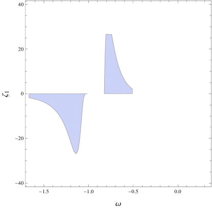
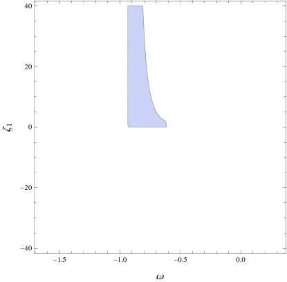
Figure 1: Stable regions in $(\omega,\zeta_{1})$ space for $\Omega_{1}^{2}$ with $c_{1}=1$ (left) and $c_{1}=5$ (right).

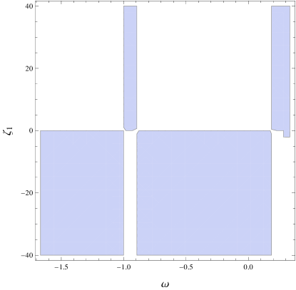
Figure 2: Stable regions in $(\omega,\zeta_{1})$ space for $\Omega_{2}^{2}$ with $c_{1}=1$ (left) and $c_{1}=-1$ (right).

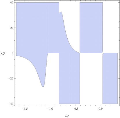
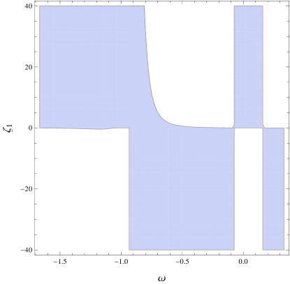
Figure 3: Stable regions in $(\omega,\zeta_{1})$ space for $\Omega_{1,2}^{2}$ with $c_{1}=1$ (left) and $c_{1}=5$ (right).

3.2 Non-Conserved EMT

Here, we analyze the stability of $f(\mathcal{G},T)$ model when EMT is not conserved. We consider generic function $f_{1}(\mathcal{G})$ and a linear form of $f_{2}(T)$ in Eq.(26) as follows

$$f(\mathcal{G},T)=f_{1}(\mathcal{G})+\kappa^{2}\chi T,$$ (30)

where $\chi$ is an arbitrary constant. Substituting in Eq.(13), we obtain

$$\rho=\tilde{\rho}_{0}a^{-3\varphi},\quad\varphi=\frac{2(1+\chi)(1+\omega)}{2+\chi(3-\omega)},$$

where $\tilde{\rho}_{0}$ is an integration constant. The perturbed field equations (3) and (20) take the following form

$$6\delta a+\kappa^{2}a_{0}^{2}\rho_{0}\left[1-\frac{\chi}{2}(\omega-3)\right]\delta\rho=0,$$ (31)

$$2\delta\ddot{a}-\frac{2}{a_{0}^{2}}\delta a+\kappa^{2}\left[\omega-\frac{\chi}{2}(1-3\omega)\right]\rho_{0}\delta\rho-\frac{96}{a_{0}^{4}}f_{1}^{\prime\prime}(\mathcal{G}_{0})\delta a^{(iv)}=0.$$ (32)

The first field equation shows the relationship between the perturbed energy density and scale factor perturbations. Eliminating $\delta\rho$ from Eqs.(31) and (32), the resulting differential equation in perturbed $a(t)$ is given by

$$2\delta\ddot{a}-\frac{2}{a_{0}^{2}}\left[1+\frac{3(2\omega-\chi(1-3\omega))}{2-\chi(\omega-3)}\right]\delta a-\frac{96}{a_{0}^{4}}f_{1}^{\prime\prime}(\mathcal{G}_{0})\delta a^{(iv)}=0.$$ (33)

In this case, the addition of static field equations yields

$$\frac{2}{a_{0}^{2}}=\kappa^{2}\rho_{0}(1+\chi)(1+\omega).$$ (34)

Inserting this value of $\frac{2}{a_{0}^{2}}$ in Eq.(33), we obtain

$$\kappa^{2}\rho_{0}[\chi(1+\chi)(1-\omega^{2})-(1+\chi)^{2}(1+\omega)(1+3\omega)]\delta a+[2(1+\chi)$$ (35)

$$+ \chi(1-\omega)]\delta\ddot{a}-12\kappa^{4}\rho_{0}^{2}[2(1+\chi)^{3}(1+\omega)^{2}+\chi(1+\chi)^{2}(1-\omega)(1+\omega)^{2}]$$

$$\times f_{1}^{\prime\prime}(\mathcal{G}_{0})\delta a^{(iv)}=0,$$

whose solution provides the following four frequencies as

$$\Upsilon^{2}_{1,2}=\frac{-2(1+\chi)-\chi(1-\omega)\pm\sqrt{[2(1+\chi)+\chi(1-\omega)]^{2}-48\kappa^{6}\rho_{0}^{3}\Delta_{4}f_{1}^{\prime\prime}(\mathcal{G}_{0})}}{24\kappa^{4}\rho_{0}^{2}[\chi(1+\chi)^{2}(\omega-1)(1+\omega)^{2}-2(1+\chi)^{3}(1+\omega)^{2}]f_{1}^{\prime\prime}(\mathcal{G}_{0})},$$

where

$$\Delta_{4} = [2(1+\chi)^{3}(1+\omega)^{2}+\chi(1+\chi)^{2}(1-\omega)(1+\omega)^{2}][(1+\chi)^{2}(1+\omega)$$

$$\times (1+3\omega)-\chi(1+\chi)(1-\omega^{2})].$$

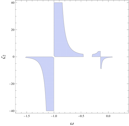
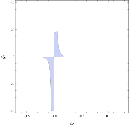
Figure 4: Stable regions in $(\omega,\zeta_{2})$ space for $\Upsilon_{1}^{2}$ with $\chi=1$ (left) and $\chi=5$ (right).

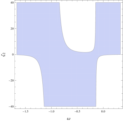
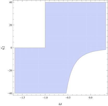
Figure 5: Stable regions in $(\omega,\zeta_{2})$ space for $\Upsilon_{2}^{2}$ with $\chi=1$ (left) and $\chi=-0.5$ (right).

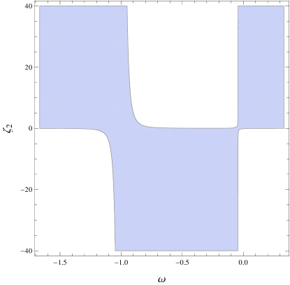
Figure 6: Stable regions in $(\omega,\zeta_{2})$ space for $\Upsilon_{1,2}^{2}$ with $\chi=1$ (left) and $\chi=5$ (right).

When $f_{1}(\mathcal{G}_{0})=0=\chi$, the frequencies $\Upsilon^{2}_{1}$ recover the GR result as obtained in the previous case while frequencies $\Upsilon^{2}_{2}$ diverge. We simplify the expression by introducing a new parameter $\zeta_{2}=-48\kappa^{6}\rho_{0}^{3}f_{1}^{\prime\prime}(\mathcal{G}_{0})$ which remains positive for $f_{1}^{\prime\prime}(\mathcal{G}_{0})<0$. Figure 4 shows stable regions against homogeneous perturbations of EU for frequencies $\Upsilon_{1}^{2}$. It is found that when $\chi=1$ (left panel), the stable EU exists for all values of $\omega$ with suitable choice of $\zeta_{2}$ while less stable regions are obtained when $\chi=5$ as shown in the right plot. In the case of non-conserved EMT, the stability regions decrease as the value of model parameter $\chi$ increases while no stable regions are observed for $\chi<0$. The regions of stability in EU for frequencies $\Upsilon^{2}_{2}$ are shown in Figure 5 for considered values of $\chi$ while stability regions for whole system is observed in Figure 6.

Now, we consider the generalized model given by

$$f(\mathcal{G},T)=f_{1}(\mathcal{G})+\kappa^{2}\chi T^{n},\quad n\neq 0.$$ (36)

Following the same procedure, we obtain the following fourth-order differential equation in perturbed $a(t)$ as follows

$$24\kappa^{4}\rho_{0}^{2}(1+\omega)^{2}\left[1+n\chi\rho_{0}^{n-1}(1-3\omega)^{n-1}\right]^{2}f_{1}^{\prime\prime}(\mathcal{G}_{0})\delta a^{(iv)}-2\delta\ddot{a}$$

$$+ \kappa^{2}\rho_{0}(1+\omega)\left(1+n\chi\rho_{0}^{n-1}(1-3\omega)^{n-1}\right)\left[1+3\left(\omega-\frac{n}{2}\chi(1-3\omega)^{n}\rho_{0}^{n-1}\right)\right.$$

$$\times \left.\left(1+n\chi(1-3\omega)^{n-1}\rho_{0}^{n-1}\left[(1+\omega)+\frac{1}{2}(1-3\omega)+(n-1)\right.\right.\right.$$

$$\times \left.\left.\left.(1+\omega)\right]\right)^{-1}\right]\delta a=0,$$

whose solution provides the following four frequencies as

$$\Xi^{2}_{1,2}=\frac{1\pm\sqrt{1-24\kappa^{6}\Delta_{5}f^{\prime\prime}_{1}(\mathcal{G}_{0})}}{24\left[\kappa^{2}\rho_{0}(1+\omega)\left(1+n\chi\rho_{0}^{n-1}(1-3\omega)^{n-1}\right)\right]^{2}f_{1}^{\prime\prime}(\mathcal{G}_{0})},$$

where

$$\Delta_{5} = \rho_{0}^{3}(1+\omega)^{3}\left(1+n\chi\rho_{0}^{n-1}(1-3\omega)^{n-1}\right)^{3}\left[1+3\left(\omega-\frac{n}{2}\chi(1-3\omega)^{n}\right.\right.$$

$$\times \left.\left.\rho_{0}^{n-1}\right)\left[1+n\chi(1-3\omega)^{n-1}\rho_{0}^{n-1}\left((1+\omega)+\frac{1}{2}(1-3\omega)+(n-1)\right.\right.\right.$$

$$\times \left.\left.\left.(1+\omega)\right)\right]^{-1}\right].$$

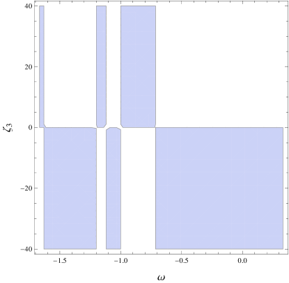
Figure 7: Stable regions in $(\omega,\zeta_{3})$ space for $\Xi_{2}^{2}$ with $n=-5$ (left) and $n=0.5$ (right).

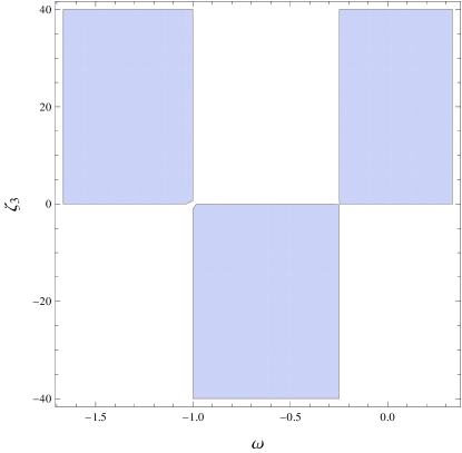
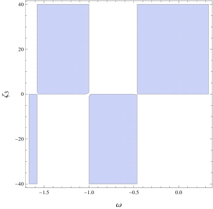
Figure 8: Stable regions in $(\omega,\zeta_{2})$ space for $\Xi_{2}^{2}$ with $n=2$ (left) and $n=5$ (right).

The graphical analysis of frequencies $\Xi_{2}^{2}$ are shown in Figures 7 and 8 where we have used $\zeta_{3}=-24\kappa^{6}f_{1}^{\prime\prime}(\mathcal{G}_{0}),~{}\kappa^{2}=1,~{}\rho_{0}=0.3$ and $\chi=1$. It is found that stable regions are obtained for all the considered values of $n$ while stable EU does not exist for the frequencies $\Xi_{1}^{2}$. In this case, the stability region of whole system is completely described by the frequencies $\Xi_{2}^{2}$. It is interesting to mention here that for $f_{1}(\mathcal{G}_{0})=0=\chi$, the frequencies $\Xi^{2}_{1}$ diverge while GR is recovered for the frequencies $\Xi^{2}_{2}$ as in the previous case.

4 Final Remarks

In this paper, we have analyzed the stability issue of EU in the context of $f(\mathcal{G},T)$ gravity which is the extension of $f(\mathcal{G})$ gravity and is based on the ground of matter-curvature coupling. Due to this coupling, the conservation law does not hold as in $f(R,T)$ gravity [7]. We have considered the isotropic and homogeneous positive curvature FRW line element with perfect fluid as matter content of the universe. The static as well as perturbed field equations are constructed against linear homogeneous perturbations which are parameterized by equation of state parameter. We have formulated the fourth-order perturbed differential equation whose solutions are analyzed for the existence and stability of EU for specific form of $f(\mathcal{G},T)=f_{1}(\mathcal{G})+f_{2}(T)$. For this choice, we have discussed both the models when EMT is conserved as well not conserved and obtained distinct results as compared to $f(\mathcal{G})$ gravity.

• We have assumed that EMT is conserved in this gravity and obtained a particular form of $f_{2}(T)$ for which the covariant divergence of EMT becomes zero. We have analyzed the regions of stability around EU and found that stable results are observed for a suitable choice of integration constant $c_{1}$.

• Two particular forms of $f_{2}(T)$ are considered for which the covariant divergence of EMT remains non-zero and the value of energy density in terms of scale factor is evaluated. It is found that stable EU exists in this case for both models if the model parameter $\chi$ is chosen appropriately.

We conclude that the stable EU universe exists against scalar homogeneous perturbations in the background of $f(\mathcal{G},T)$ for all values of the equation of state parameter if the model parameters are chosen suitably. Einstein universe against vector perturbations (comoving dimensionless vorticity vector) are stable for all equations of state on all scales since any initial vector perturbations remain frozen. The mechanism for stability analysis of EU against tensor perturbations (comoving dimensionless traceless shear tensor) suggests that these fluctuations may not break the stability of EU in the background of $f(\mathcal{G},T)$ gravity [12]. It would be interesting to investigate complete analysis of tensor as well as inhomogeneous perturbations in this gravity which will be helpful to explore the EU. It is worth mentioning here that our results reduce to $f(\mathcal{G})$ gravity in the absence of matter-curvature coupling [18].

References

- [1] Calcagni, G., Tsujikawa, S. and Sami, M.: Class. Quantum Grav. 22(2005)3977; De Felice, A., Hindmarsh, M. and Trodden, M.: J. Cosmol. Astropart. Phys. 08(2006)005.
- [2] Metsaev, R.R. and Tseytlin, A.A.: Nucl. Phys. B 293(1987)385; Antoniadis, I., Rizos, J. and Tamvakis, K.: Nucl. Phys. B 415(1994)497; Kanti, P., Rizos, J. and Tamvakis, K.: Phys. Rev. D 59(1999)083512; Nojiri, S. and Odintsov, S.D.: Int. J. Geom. Meth. Mod. Phys. 4(2007)115.
- [3] Nojiri, S. and Odintsov, S.D.: Phys. Lett. B 631(2005)1.
- [4] Cognola, G. et al.: Phys. Rev. D 73(2006)084007.
- [5] De Felice, A. and Tsujikawa, S.: Phys. Lett. B 675(2009)1.
- [6] De Felice, A. and Tsujikawa, S.: Phys. Rev. D 80(2009)063516.
- [7] Harko, T. et al.: Phys. Rev. D 84(2011)024020.
- [8] Sharif, M. and Ikram, A.: Eur. Phys. J. C 76(2016)640.
- [9] Eddington, A.S.: Mon. Not. R. Astron. Soc. 90(1930)668.
- [10] Harrison, E.R.: Rev. Mod. Phys. 39(1967)862.
- [11] Gibbons, G.W.: Nucl. Phys. B 292(1987)784.
- [12] Barrow, J.D. et al.: Class. Quantum Grav. 20(2003)L155.
- [13] Ellis, G.F.R. and Maartens, R.: Class. Quantum Grav. 21(2004)223; Ellis, G.F.R., Murugan, J. and Tsagas, C.G.: Class. Quantum Grav. 21(2004)233.
- [14] Gergely, L.Á. and Maartens, R.: Class. Quantum. Grav. 19(2002)213; Gruppuso, A. Roessl, E. and Shaposhnikov, M.: J. High Energy Phys. 08(2004)011; Böhmer, C.G.: Class. Quantum. Grav. 21(2004)1119; Mulryne, D.J. et al.: Phys. Rev. D 71(2005)123512; Atazadeh, K. and Darabi, F.: Phys. Lett. B 744(2015)363; Zhang, K. et al.: Phys. Lett. B 758(2016)37.
- [15] Böhmer, C.G., Hollenstein, L. and Lobo, F.S.N.: Phys. Rev. D 76(2007)084005.
- [16] Goswami, R., Goheer, N. and Dunsby, P.K.S.: Phys. Rev. D 78(2008)044011.
- [17] Goheer, N. Goswami, R. and Dunsby, P.K.S.: Class. Quantum Grav. 26(2009)105003.
- [18] Böhmer, C.G. and Lobo, F.S.N.: Phys. Rev. D 79(2009)067504.
- [19] Böhmer, C.G., Lobo, F.S.N. and Tamanini, N.: Phys. Rev. D 88(2013)104019.
- [20] Li, J.T., Lee, C.C. and Geng, C.Q.: Eur. Phys. J. C 73(2013)2315.
- [21] Huang, H., Wu, P. and Yu, H.: Phys. Rev. D 89(2014)103521.
- [22] Huang, H., Wu, P. and Yu, H.: Phys. Rev. D 91(2015)023507.
- [23] Böhmer, C.G., Tamanini, N. and Wright, M.: Phys. Rev. D 92(2015)124067.
- [24] Darabi, F., Heydarzade, Y. and Hajkarim, F.: Can. J. Phys. 93(2015)1566.
- [25] Shabani, H. and Ziaie, A.H.: arXiv:1606.07959.
- [26] Landau, L.D. and Lifshitz, E.M.: The Classical Theory of Fields (Pergamon Press, 1971).
- [27] Ade, P.A.R. et al.: Astron. Astrophys. 594(2016)A13.
- [28] Li, B., Barrow, J.D. and Mota, D.F.: Phys. Rev. D 76(2007)044027.