Exploring cosmic origins with CORE: effects of observer peculiar motion

Abstract

We discuss the effects on the cosmic microwave background (CMB), cosmic infrared background (CIB), and thermal Sunyaev-Zeldovich effect due to the peculiar motion of an observer with respect to the CMB rest frame, which induces boosting effects. After a brief review of the current observational and theoretical status, we investigate the scientific perspectives opened by future CMB space missions, focussing on the Cosmic Origins Explorer (CORE) proposal. The improvements in sensitivity offered by a mission like CORE, together with its high resolution over a wide frequency range, will provide a more accurate estimate of the CMB dipole. The extension of boosting effects to polarization and cross-correlations will enable a more robust determination of purely velocity-driven effects that are not degenerate with the intrinsic CMB dipole, allowing us to achieve an overall signal-to-noise ratio of 13; this improves on the Planck detection and essentially equals that of an ideal cosmic-variance-limited experiment up to a multipole $\ell\simeq 2000$. Precise inter-frequency calibration will offer the opportunity to constrain or even detect CMB spectral distortions, particularly from the cosmological reionization epoch, because of the frequency dependence of the dipole spectrum, without resorting to precise absolute calibration. The expected improvement with respect to COBE-FIRAS in the recovery of distortion parameters (which could in principle be a factor of several hundred for an ideal experiment with the CORE configuration) ranges from a factor of several up to about 50, depending on the quality of foreground removal and relative calibration. Even in the case of $\simeq 1$ % accuracy in both foreground removal and relative calibration at an angular scale of $1^{\circ}$, we find that dipole analyses for a mission like CORE will be able to improve the recovery of the CIB spectrum amplitude by a factor $\simeq 17$ in comparison with current results based on COBE-FIRAS. In addition to the scientific potential of a mission like CORE for these analyses, synergies with other planned and ongoing projects are also discussed.

1 Introduction

The peculiar motion of an observer with respect to the cosmic microwave background (CMB) rest frame gives rise to boosting effects (the largest of which is the CMB dipole, i.e., the multipole $\ell=1$ anisotropy in the Solar System barycentre frame), which can be explored by future CMB missions. In this paper, we focus on peculiar velocity effects and their relevance to the Cosmic Origins Explorer (CORE) experiment. CORE is a satellite proposal dedicated to microwave polarization and submitted to the European Space Agency (ESA) in October 2016 in response to a call for future medium-sized space mission proposals for the M5 launch opportunity of ESA’s Cosmic Vision programme.

This work is part of the Exploring Cosmic Origins (ECO) collection of articles, aimed at describing different scientific objectives achievable with the data expected from a mission like CORE. We refer the reader to the CORE proposal [CORE2016] and to other dedicated ECO papers for more details, in particular the mission requirements and design paper [delabrouille_etal_ECO] and the instrument paper [debernardis_etal_ECO], which provide a comprehensive discussion of the key parameters of CORE adopted in this work. We also refer the reader to the paper on extragalactic sources [2016arXiv160907263D] for an investigation of their contribution to the cosmic infrared background (CIB), which is one of the key topics addressed in the present paper, as well as the papers on $B$-mode component separation [baccigalupi_etal_ECO] for a stronger focus on polarization, and mitigation of systematic effects [ashdown_etal_ECO] for further discussion of potential residuals included in some analyses presented in this work. Throughout this paper we use the CORE specifications summarised in Table 1.

Channel	Beam	$N_{\rm det}$	$\Delta T$	$\Delta P$	$\Delta I$	$\Delta I$	$\Delta y\times 10^{6}$
[GHz]	[arcmin]		[$\mu$K.arcmin]	[$\mu$K.arcmin]	[$\mu$KRJ.arcmin]	[kJy sr-1.arcmin]	[$y_{\rm SZ}$.arcmin]
60	17.87	48	7.5	10.6	6.81	0.75	$-$1.5
70	15.39	48	7.1	10	6.23	0.94	$-$1.5
80	13.52	48	6.8	9.6	5.76	1.13	$-$1.5
90	12.08	78	5.1	7.3	4.19	1.04	$-$1.2
100	10.92	78	5.0	7.1	3.90	1.2	$-$1.2
115	9.56	76	5.0	7.0	3.58	1.45	$-$1.3
130	8.51	124	3.9	5.5	2.55	1.32	$-$1.2
145	7.68	144	3.6	5.1	2.16	1.39	$-$1.3
160	7.01	144	3.7	5.2	1.98	1.55	$-$1.6
175	6.45	160	3.6	5.1	1.72	1.62	$-$2.1
195	5.84	192	3.5	4.9	1.41	1.65	$-$3.8
220	5.23	192	3.8	5.4	1.24	1.85	…
255	4.57	128	5.6	7.9	1.30	2.59	3.5
295	3.99	128	7.4	10.5	1.12	3.01	2.2
340	3.49	128	11.1	15.7	1.01	3.57	2.0
390	3.06	96	22.0	31.1	1.08	5.05	2.8
450	2.65	96	45.9	64.9	1.04	6.48	4.3
520	2.29	96	116.6	164.8	1.03	8.56	8.3
600	1.98	96	358.3	506.7	1.03	11.4	20.0
Array		2100	1.2	1.7			0.41

Table 1: Proposed CORE-M5 frequency channels. The sensitivity is estimated assuming $\Delta\nu/\nu=30\,\%$ bandwidth, 60 % optical efficiency, total noise of twice the expected photon noise from the sky and the optics of the instrument being at 40 K. The second column gives the FWHM resolution of the beam. This configuration has 2100 detectors, about 45 % of which are located in CMB channels between 130 and 220 GHz. Those six CMB channels yield an aggregated CMB sensitivity of $2\,\mu$K.arcmin ($1.7\,\mu$K.arcmin for the full array).

The analysis of cosmic dipoles is of fundamental relevance in cosmology, being related to the isotropy and homogeneity of the Universe at the largest scales. In principle, the observed dipole is a combination of various contributions, including observer motion with respect to the CMB rest frame, the intrinsic primordial (Sachs-Wolfe) dipole and the Integrated Sachs-Wolfe dipole as well as dipoles from astrophysical (extragalactic and Galactic) sources. The interpretation that the CMB dipole is mostly (if not fully) of kinematic origin has strong support from independent studies of the galaxy and cluster distribution, in particular via the measurements of the so-called clustering dipole. According to the linear theory of cosmological perturbations, the peculiar velocity of an observer (as imprinted in the CMB dipole) should be related to the observer’s peculiar gravitational acceleration via $\vec{v}_{\rm lin}=\beta_{\rm rd}\vec{g}_{\rm lin}$, where $\beta_{\rm rd}\simeq\Omega_{\rm m}^{0.55}/b_{\rm g}$ is also know as the redshift-space distortion parameter ($b_{\rm g}$ and $\Omega_{\rm m}$ being, respectively, the bias of the particular galaxy sample and the matter density parameter at the present time). The peculiar velocity and acceleration of, for instance, the Local Group treated as one system, i.e., as measured from its barycentre, should thus be aligned and have a specific relation between amplitudes. The former fact has been confirmed from analyses of many surveys over the last three decades, such as IRAS [1987MNRAS.228P...5H, 1992ApJ...397..395S], 2MASS [2003ApJ...598L...1M, 2006MNRAS.368.1515E], or galaxy cluster samples [1996ApJ...460..569B, 1998ApJ...500....1P]. As far as the amplitudes are concerned, the comparison has been used to place constraints on the $\beta_{\rm rd}$ parameter [1996ApJ...460..569B, 2000MNRAS.314..375R, 2006MNRAS.368.1515E, 2006MNRAS.373.1112B, 2011ApJ...741...31B], totally independent of those from redshift-space distortions observed in spectroscopic surveys. In this context, confirming the kinematic origin of the CMB dipole, through a comparison accounting for our Galaxy’s motion in the Local Group and the Sun’s motion in the Galaxy (see e.g., Refs. [1999AJ....118..337C, 2012MNRAS.427..274S]), would provide support for the standard cosmological model, while finding any significant deviations from this assumption could open up the possibility for other interpretations (see e.g., Refs. [2013PhRvD..88h3529W, 2016JCAP...06..035B, 2016JCAP...12..022G, Roldan:2016ayx]).

Cosmic dipole investigations of more general type have been carried out in several frequency domains [2012MNRAS.427.1994G], where the main signal comes from various types of astrophysical sources differently weighted in different shells in redshift. An example are dipole studies in the radio domain, pioneered by Ref. [1984MNRAS.206..377E] and recently revisited by Ref. [2013A&A...555A.117R] performing a re-analysis of the NRAO VLA Sky Survey (NVSS) and the Westerbork Northern Sky Survey, as well as by Refs. [2015APh....61....1T, 2015MNRAS.447.2658T] using NVSS data alone. Prospects to accurately measure the cosmic radio dipole with the Square Kilometre Array have been studied by Ref. [2015aska.confE..32S]. Perspectives on future surveys jointly covering microwave/millimeter and far-infrared wavelengths aimed at comparing CMB and CIB dipoles have been presented in Ref. [2011ApJ...734...61F]. The next decades will see a continuous improvement of cosmological surveys in all bands. For the CMB, space observations represent the best, if not unique, way to precisely measure this large-scale signal. It is then important to consider the expectations from (and the potential issues for) future CMB surveys beyond the already impressive results produced by Planck.

In addition to the dipole due to the combination of observer velocity and Sachs-Wolfe and intrinsic (see ref. [2017arXiv170400718M] for a recent study) effects, a moving observer will see velocity imprints on the CMB due to Doppler and aberration effects [Challinor:2002zh, Burles:2006xf], which manifest themselves in correlations between the power at subsequent multipoles of both temperature and polarization anisotropies. Precise measurements of such correlations [Kosowsky:2010jm, Amendola:2010ty] provide important consistency checks of fundamental principles in cosmology, as well as an alternative and general way to probe observer peculiar velocities [2014A&A...571A..27P, Roldan:2016ayx]. This type of analysis can in principle be extended to thermal Sunyaev-Zeldovich (tSZ) [2005A&A...434..811C] and CIB signals. We will discuss how these investigations could be improved when applied to data expected from a next generation of CMB missions, exploiting experimental specifications in the range of those foreseen for LiteBIRD [2016SPIE.9904E..0XI] and CORE.

Since the results from COBE [1992ApJ...397..420B], no substantial improvements have been achieved in the observations of the CMB spectrum at $\nu\,\lower 2.0pt\hbox{${>\atop\hbox{\raise 4.0pt\hbox{$\sim$}}}$}\,30$ GHz. Absolute spectral measurements rely on ultra-precise absolute calibration. FIRAS [1996ApJ...473..576F] achieved an absolute calibration precision of 0.57 mK, with a typical inter-frequency calibration accuracy of $0.1$ mK in one decade of frequencies around 300 GHz. The amplitude and shape of the CIB spectrum, measured by FIRAS [Fixsen:1998kq], is still not well known. Anisotropy missions, like CORE, are not designed to have an independent absolute calibration, but nevertheless can investigate the CMB and CIB spectra by looking at the frequency spectral behaviour of the dipole amplitude [DaneseDeZotti1981, Balashev2015, 2016JCAP...03..047D, Planck_inprep]. Unavoidable spectral distortions are predicted as the result of energy injections in the radiation field occurring at different cosmic times, related to the origin of cosmic structures and to their evolution, or to the different evolution of the temperatures of matter and radiation (for a recent overview of spectral distortions within standard $\Lambda$CDM, see Ref. [2016MNRAS.460..227C]). For quantitative forecasts we will focus on well-defined types of signal, namely Bose-Einstein (BE) and Comptonization distortions [1969Ap&SS...4..301Z, 1970Ap&SS...7...20S]; however, one should also be open to the possible presence of unconventional heating sources, responsible in principle for imprints larger than (and spectral shapes different from) those mentioned above, and having parameters that could be constrained through analysis of the CMB spectrum. Deciphering such signals will be a challenge, but holds the potential for important new discoveries and for constraining unexplored processes that cannot be probed by other means. At the same time, a better determination of the CIB intensity greatly contributes to our understanding of the dust-obscured star-formation phase of galaxy evolution.

The rest of this paper is organised as follows. In Sect. 2 we quantify the accuracy of a mission like CORE for recovering the dipole direction and amplitude separately at a given frequency, focussing on a representative set of CORE channels. Accurate relative calibration and foreground mitigation are crucial for analysing CMB anisotropy maps. In Sect. 3 we describe a parametric approach to modelling the pollution of theoretical maps with potential residuals. The analysis in Sect. 2 is then extended in Sect. 4 to include a certain level of residuals. The study throughout these sections is carried out in pixel domain.

In Sect. 5 we describe the imprints at $\ell>1$ due to Doppler and aberration effects, which can be measured in harmonic space. Precise forecasts based on CORE specifications are presented and compared with those expected from LiteBIRD. The intrinsic signature of a boost in Sunyaev-Zeldovich and CIB maps from CORE is also discussed in this section.

In Sect. 6 we study CMB spectral distortions and the CIB spectrum through the analysis of the frequency dependence of the dipole distortion; we introduce a method to extend predictions to higher multipoles, coupling higher-order effects and geometrical aspects. The theoretical signals are compared with sensitivity at different frequencies, in terms of angular power spectrum, for a mission like CORE. In Sect. 7 we exploit the available frequency coverage through simulations to forecast CORE’s sensitivity to the spectral distortion parameters and the CIB spectrum amplitude, considering the ideal case of perfect relative calibration and foreground subtraction; however, we also parametrically quantify the impact of potential residuals, in order to define the requirements for substantially improve the results beyond those from FIRAS.

In Sect. LABEL:sec:end we summarise and discuss the main results. The basic concepts and formalisms are introduced in the corresponding sections, while additional information and technical details are provided in several dedicated appendices for sake of completeness.

2 The CMB dipole: forecasts for CORE in the ideal case

A relative velocity, $\beta\equiv v/c$, between an observer and the CMB rest frame induces a dipole (i.e., $\ell=1$ anisotropy) in the temperature of the CMB sky through the Doppler effect. Such a dipole is likely dominated by the velocity of the Solar System, $\vec{\beta_{\rm S}}$, with respect to the CMB (Solar dipole), with a seasonal modulation due to the velocity of the Earth/satellite, $\vec{\beta_{\rm o}}$, with respect to the Sun (orbital dipole). In this work we neglect the orbital dipole (which may indeed be used for calibration), thus hereafter we will denote with $\vec{\beta}$ the relative velocity of the Solar dipole.

In this section we forecast the ability to recover the dipole parameters (amplitude and direction) by performing a Markov chain Monte Carlo (MCMC) analysis in the ideal case (i.e., without calibration errors or sky residuals). Results including systematics are given in Sect. 4. We test the amplitude of the parameter errors against the chosen sampling resolution and we probe the impact of both instrumental noise and masking of the sky. We consider the “Planck common mask 76” (in temperature), which is publicly available from the Planck Legacy Archive (PLA) [PLArefESA], and keeps 76 % of the sky, avoiding the Galactic plane and regions at higher Galactic latitudes contaminated by Galactic or extragalactic sources. We exploit here an extension of this mask that excludes all the pixels at $|b|\leq 30^{\circ}$.

Additionally, we explore the dipole reconstruction ability for different frequency channels, specifically 60, 100, 145, and 220 GHz. We finally investigate the impact of spectral distortions (see Sects. 6 and 7), treating the specific case of a BE spectrum (with chemical potential $\mu_{0}=1.4\times 10^{-5}$, which is several times smaller than FIRAS upper limits).

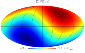
Figure 1: Map of the CMB dipole used in the simulations, corresponding to an amplitude $A=3.3645$ mK and a dipole direction defined by the Galactic coordinates $b_{0}=48.24^{\circ}$ and $l_{0}=$ $264.00^{\circ}$. The map is in Galactic coordinates and at a resolution of $\simeq 3.4$ arcmin, corresponding to HEALPix $N_{\rm side}=1024$.

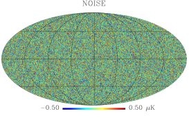
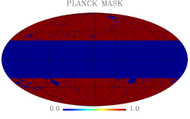
Figure 2: Instrumental noise map and Planck Galactic mask (extended to cut out $\pm 30^{\circ}$ of the Galactic plane) employed in the simulations. The noise map corresponds to 7.5 $\mu$K.arcmin, as expected for the 60-GHz band. The Map is in Galactic coordinates and at resolution of $\simeq 3.4$ arcmin, corresponding to HEALPix $N_{\rm side}=1024$.

We write the dipole in the form:

$$d(\hat{n})=A\,\hat{n}\cdot\hat{n}_{0}+T_{0},$$ (2.1)

where $\hat{n}$ and $\hat{n}_{0}$ are the unit vectors defined respectively by the Galactic longitudes and latitudes $(l,b)$ and $(l_{0},b_{0})$. In Fig. 1 we show the dipole map we have used in our simulations, generated assuming the best-fit values of the measurements of the dipole amplitude, $A=(3.3645\pm 0.002)$ mK, and direction, $l_{0}=264.00^{\circ}\pm 0.03^{\circ}$ and $b_{0}=48.24^{\circ}\pm 0.02^{\circ}$, found in the Planck (combined result from the High Frequency Instrument, HFI, and Low Frequency Instrument, LFI) 2015 release [2016A&A...594A...1P, 2016A&A...594A...5P, 2016A&A...594A...8P]. Assuming the dipole to be due to velocity effects only, its amplitude corresponds to $\beta\equiv|\vec{\beta}|\equiv v/c=A/T_{0}=1.2345\times 10^{-3}$, with $T_{0}=2.72548\pm 0.00057\,$K being the present-day temperature of the CMB [2009ApJ...707..916F]. In Fig. 2 we show the instrumental noise map and the Planck Galactic mask employed in the simulations. The noise map corresponds to 7.5 $\mu$K.arcmin, as expected for the 60-GHz band.

We calculate the likelihoods for the parameters $A$, $l_{0}$, $b_{0}$ and $T_{0}$ using the publicly available COSMOMC generic sampler package [2002PhRvD..66j3511L, Metropolis53, Hastings70]. While the monopole $T_{0}$ is not an observable of interest in this context, we include it as a free parameter, to verify any degeneracy with the other parameters and for internal consistency checks.

To probe the dependence of the parameter error estimates on the sampling resolution, we investigate the dipole reconstruction at HEALPix [2005ApJ...622..759G] $N_{\rm side}=128$, 256, 512, and 1024, eventually including the noise and the Galactic mask. The reference frequency channel for this analysis is the 60-GHz band. The corresponding likelihoods are collected in Appendix LABEL:sec:Likelihoods (see Fig. LABEL:fig:conflevel128+1024) for the same representative values of $N_{\rm side}$ (see also Table LABEL:table:conflevel128+1024 for the corresponding 68% confidence levels).

In Fig. 4 we plot the 1 $\sigma$ uncertainties on the parameter estimates as functions of the HEALPix $N_{\rm side}$ value. We find that the pixelization error due to the finite resolution is dominant over the instrumental noise at any $N_{\rm side}$. This means that we are essentially limited by the sampling resolution. As expected, the impact of noise is negligible, although the effect of reducing the effective sky fraction is relevant. In fact, the presence of the Galactic mask results in larger errors (for all parameters) and introduces a small correlation between the parameters $A$ and $b_{0}$, as clearly shown in these plots.

The likelihood results for some of the different frequencies under analysis are collected in Figs. LABEL:fig:conflevel100220 of Appendix LABEL:sec:Likelihoods (see also Table LABEL:table:conflevel60220 for the 68% confidence levels at the four considered frequencies). Here we keep the resolution fixed at HEALPix $N_{\rm side}=1024$ and consider both noise level and choice of Galactic mask. We find that the dipole parameter estimates do not significantly change among the frequency channels, which is clearly due to the sub-dominant effect of the noise.

As a last test of the ideal case, we compare the dipole parameter reconstruction between the cases of a pure blackbody (BB) spectrum and a BE-distorted spectrum. The comparison of the likelihoods is presented in Fig. LABEL:fig:conflevelBE of Appendix LABEL:sec:Likelihoods (see also Table LABEL:table:conflevelBE for the corresponding 68% confidence levels). This analysis shows that the parameter errors are not affected by the spectral distortion and that the direction of the dipole is successfully recovered. The difference found in the amplitude value is consistent with the theoretical difference of about 76 nK.

3 Parametric model for potential foreground and calibration residuals in total intensity

In the previous section we showed that in the ideal case of pure noise, i.e., assuming perfect foreground subtraction and calibration (and the absence of systematic effects) in the sky region being analysed, pixel-sampling limitation dominates over noise limitation.

Clearly, specific component-separation and calibration methods (and implementations) introduce specific types of residuals. Rather than trying to accurately characterise them (particularly in the view of great efforts carried out in the last decade for specific experiments and the progress that is expected over the coming years), we implemented a simple toy model to parametrically estimate the potential impact of imperfect foreground subtraction and calibration in total intensity (i.e., in temperature). This includes using some of the Planck results and products made publicly available through the PLA.

The PLA provides maps in total intensity (or temperature) at high resolution ($N_{\rm side}=2048$) of global foregrounds at each Planck frequency (here we use those maps based on the COMMANDER method). It provides also suitable estimates of the zodiacal light emission (ZLE) maps (in temperature) from Planck-HFI. Our aim is to produce templates of potential foreground residuals that are simply scalable in amplitude according to a tunable parameter. In order to estimate such emission at CORE frequencies, without relying on particular sky models, we simply interpolate linearly (in logarithmic scale, i.e., in ${\rm log}(\nu)$–${\rm log}(T))$ pixel by pixel the foreground maps and the ZLE maps, and linearly extrapolate the ZLE maps at $\nu<100$ GHz. We then create a template of signal sky amplitude at each CORE frequency, adding the absolute values in each pixel of these foreground and ZLE maps and of the CMB anisotropy map available at the same resolution in the PLA (we specifically use that based on COMMANDER). Since for this analysis we are not interested in separating CMB and astrophysical emission at $\ell\geq 3$, we then generate templates from these maps, extracting the $a_{lm}$ modes for $\ell\leq 2$ only. These templates are then degraded to the desired resolution. Finally, we generate maps of Gaussian random fields at each CORE frequency, with rms amplitude given by these templates, $T_{\rm amp,for}$, multiplied by a tunable parameter, $E_{\rm for}$, which globally characterizes the potential amplitude of foreground residuals after component separation. Clearly, the choice of reasonable values of $E_{\rm for}$ depends on the resolution being considered (or on the adopted pixel size), with the same value of $E_{\rm for}$ but at smaller pixel size implying less contamination at a given angular scale.

Planck maps reveal, at least in temperature, a greater complexity in the sky than obtained by previous experiments. The large number of frequencies of CORE is in fact designed to accurately model foreground emission components with a precision much better than Planck’s. Also, at least in total intensity, ancillary information will come in the future from a number of other surveys, ranging from radio to infrared frequencies.

The target for CORE in the separation of diffuse polarised foreground emission corresponds to $E_{\rm for}\simeq 0.01$, i.e., to $\simeq 1$ % precision at the map level for angular scales larger than about $1^{\circ}$ (i.e., up to multipoles $\ell\,\lower 2.0pt\hbox{${<\atop\hbox{\raise 4.0pt\hbox{$\sim$}}}$}\,200$), where the main information on primordial $B$-modes is contained, while at larger multipoles the main limitation comes from lensing subtraction and characterization and secondarily through control of extragalactic source contributions. We note also that comparing CMB anisotropy maps available from the PLA at $N_{\rm side}=2048$ derived with four different component-separation methods and degraded to various resolutions, shows that the rms of the six difference maps does not scale strongly with the adopted pixel size, at least if we exclude regions close to the Galactic plane. For example, outside the Planck common mask 76, if we pass from $N_{\rm side}=2048$ to $N_{\rm side}=256$ or $64$, i.e., increasing the pixel linear size by a factor of 8 or 32 (with the exception of the comparison of SEVEM versus SMICA), the rms values of the cross-comparisons range from about 8–9 $\mu$K to about 3–5 $\mu$K, i.e., a decreases by a factor of only about 2.5. This suggests that, at least for temperature analyses, the angular scale adopted to set $E_{\rm for}$ is not so critical.

Data calibration represents one of the most delicate aspects of CMB experiments. The quality of CMB anisotropy maps does not rely on absolute calibration of the signal (as it would, for example, in experiments dedicated to absolute measurements of the CMB temperature, i.e., in the direct determination of the CMB spectrum). However, the achievement of very high accuracy in the relative calibration of the maps (sometimes referred to as absolute calibration of the anisotropy maps), as well as the inter-frequency calibration of the maps taken in different bands, is crucial for enabling the scientific goals of CMB projects. Although this calibration step could in principle benefit from the availability of precise instrumental reference calibrators (implemented for example in FIRAS [1999ApJ...512..511M] and foreseen in PIXIE [2011JCAP...07..025K], or – but with much less accurate requirements – in Planck-LFI [2009JInst...4T2006V]), this is not necessary for anisotropy experiments, as shown for example by WMAP and Planck-HFI. This represents a huge simplification in the design of anisotropy experiments with respect to absolute temperature ones. Planck demonstrated the possibility to achieve relatively calibration of anisotropy data at a level of accuracy of about 0.1 % up to about 300 GHz, while recent analyses of planet flux density measurements and modelling [2016arXiv161207151P] indicate the possibility to achieve a calibration accuracy of $\simeq 1$ % even above 300 GHz, with only moderate improvements over what is currently realised.

The goal of CORE is to achieve a calibration accuracy level around 0.01 %, while the requirement of $0.1$ % is clearly feasible on the basis of current experiments, with some possible relaxation at high frequencies. Methods for improving calibration are fundamental in astrophysical and cosmological surveys, and clearly critical in CMB experiments. In principle, improvements in various directions can be pursued: from a better characterization of all instrument components to cross-correlation between different CMB surveys; from the implementation of external precise artificial calibration sources to the search for a better characterization (and increasing number) of astronomical calibration sources; and, in general, with the improvement of data analysis methods.

To parametrically model potential residuals due to imperfect calibration we follow an approach similar to that described above for foreground contamination. We note that calibration uncertainty implies an error proportional to the global effective (anisotropy in our case) signal. We therefore produce templates as described above, but do so by adding the foreground, ZLE, and CMB anisotropy maps, keeping their signs and maintaining all the $a_{lm}$ modes contained in the maps. The absolute values of these templates are then multiplied by a tunable parameter, $E_{\rm cal}$ (possibly dependent on frequency), which globally characterizes the amplitude of potential residuals arising from imperfect calibration. These are then used to define the pixel-by-pixel rms amplitudes, which are adopted to construct maps, $T_{\rm res,cal}$, of Gaussian random fields at each CORE frequency.

In fact, we might also expect calibration errors to affect the level of foreground residuals. Hence, as a final step, we include in the model a certain coupling between the two types of residuals. At each frequency, we multiply the above simulated maps of foreground residuals by $(1+T_{\rm res,cal}/T_{\rm amp,for})$.

4 The CMB dipole: forecasts for CORE including potential residuals

We now extend the analysis presented in Sect. 2 by including two sources of systematic effects, namely calibration errors and sky foreground residuals. We consider two pairs of calibration uncertainty and sky residuals (parameterised by $E_{\rm for}=0.04$ and $E_{\rm cal}=0.004$, and by $E_{\rm for}=0.64$ and $E_{\rm cal}=0.064$) at $N_{\rm side}=1024$ in order to explore different resolutions through pixel degradation. Rescaled to $N_{\rm side}=64$, the two cases correspond to a set-up respectively better and worse by a factor of 4 with respect to the case $E_{\rm cal}=10^{-3}$ and $E_{\rm for}=10^{-2}$.

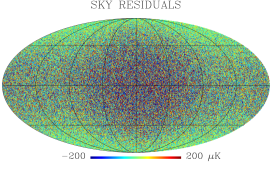
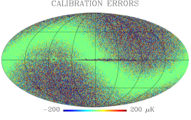
Figure 3: Sky residual and calibration error maps (in Galactic coordinates) in the 60-GHz band employed in the simulations. Their amplitudes correspond to the pessimistic case, $E_{\rm for}=0.64$ and $E_{\rm cal}=0.064$, for maps at resolution HEALPix $N_{\rm side}=1024$.

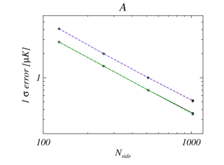
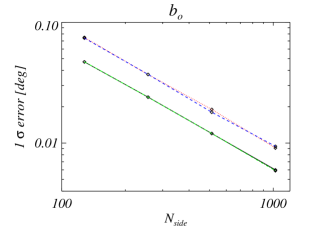
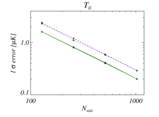
Figure 4: 1 $\sigma$ errors as function of HEALPix $N_{\rm side}$ values for the parameters $A$, $b_{0}$, $l_{0}$, and $T_{0}$: dipole-only (solid black line); dipole+noise (green dot-dashed line); dipole+noise+mask (red dotted line); and dipole+noise+mask+systematics (blue dashed line). The chosen frequency channel is 60 GHz and the noise map corresponds to 7.5 $\mu$K.arcmin. The adopted mask is the Planck Galactic mask extended to cut out $\pm 30^{\circ}$ of the Galactic plane. The systematics correspond to the pessimistic expectation of calibration errors and sky (foreground, etc.) residuals. Notice that the pixelization error, due to the finite map resolution, is dominant over the noise for any $N_{\rm side}$. While the impact of noise and systematics is negligible, we find that the effect of reducing the effective sky fraction is important.

In Fig. 3 we display the maps used in the simulations (for the 60-GHz band). The amplitudes correspond to the worse expected case; the most optimistic case is not shown, since the amplitude is just rescaled by a factor 16. The corresponding likelihood plots and 68% confidence levels are collected in Appendix LABEL:sec:Likelihoods.

We find that the impact of systematic effects on the parameter errors is negligible. In fact, as shown in Fig. 4, calibration errors and sky residuals do not noticeably worsen the 1 $\sigma$ uncertainty at any sampling resolution. Furthermore, the frequency analysis confirms that the impact of systematic effects is not relevant in any of the bands under consideration (from 60 to 220 GHz).

While the effect of the systematics studied here on the precision of the parameter reconstruction is negligible, we find instead that they may have a moderate impact on the accuracy, introducing a bias in the central values of the estimates. Nonetheless, the bias is usually buried within the 1 $\sigma$ error, with the marginal exception of the estimate of $l_{0}$ for the 220-GHz band (in the case of pessimistic systematics).

In conclusion, our results show that the dipole recovery (in both amplitude $A$ and direction angles $b_{0}$ and $l_{0}$) is completely dominated by the sky sampling resolution. We find that: the noise impact is negligible; the reduction of the sky fraction due to the presence of the Galactic mask impacts on the parameter error amplitude by increasing the 1 $\sigma$ errors on $A$, $b_{0}$ and $l_{0}$ by a factor of about 1.5, 1.6, and 1.9, respectively; and the effect of systematics slightly worsens the accuracy of the MCMC chain without affecting the error estimate.

The main point of our analysis is that, in order to achieve an increasing precision in the dipole reconstruction, high resolution measurements are required, in particular when a sky mask has to be applied. This is especially relevant for dipole spectral distortion analyses, based on the high-precision, multi-frequency observations that are necessary to study the tiny signals expected.

5 Measuring Doppler and aberration effects in different maps

5.1 Boosting effects on the CMB fields

As discussed in the previous sections, a relative velocity between an observer and the CMB rest frame induces a dipole in the CMB temperature through the Doppler effect. The CMB dipole, however, is completely degenerate with an intrinsic dipole, which could be produced by the Sachs-Wolfe effect at the last-scattering surface due to a large-scale dipolar Newtonian potential [Roldan:2016ayx]. For $\Lambda$CDM such a dipole should be of order of the Sachs-Wolfe plateau amplitude (i.e., $10^{-5}$) [2008PhRvD..78h3012E, 2008PhRvD..78l3529Z], nevertheless the dipole could be larger in the case of more exotic models. In addition to the dipole, a moving observer will also see velocity imprints at $\ell>1$ in the CMB due to Doppler and aberration effects [Challinor:2002zh, Burles:2006xf]. Such effects can be measured as correlations among different $\ell$s, as has been proposed in Refs. [Kosowsky:2010jm, Amendola:2010ty, Notari:2011sb] and subsequently demonstrated in Ref. [2014A&A...571A..27P].

The aberration effect changes the arrival direction of photons from $\hat{n}^{\prime}$ to $\hat{n}$, which, at linear order in $\beta$, is completely degenerate with a lensing dipole. The Doppler effect modulates the CMB (an effect that is partly degenerate with an intrinsic CMB dipole) changing the specific intensity $I^{\prime}$ in the CMB rest frame to the intensity $I$ in the observer’s frame by a multiplicative, direction-dependent factor as [1986rpa..book.....R, Challinor:2002zh]

$$I^{\prime}(\nu^{\prime},\,\hat{n}^{\prime})=I(\nu,\,\hat{n})\left(\frac{\nu^{\prime}}{\nu}\right)^{3},$$ (5.1)

where

$$\nu\,=\,\nu^{\prime}\,\gamma\,\big{(}1+\vec{\beta}\cdot\hat{n}^{\prime}\big{)}\,,\qquad\hat{n}\,=\,\frac{\hat{n}^{\prime}+\left[\gamma\,\beta+(\gamma-1)\big{(}\hat{n}^{\prime}\cdot\hat{\beta}\big{)}\right]\hat{\beta}}{\gamma(1+\vec{\beta}\cdot\hat{n}^{\prime})}\,,$$ (5.2)

with $\gamma\equiv(1-\vec{\beta}^{2})^{-1/2}$. The temperature and polarization fields $X(\hat{n})$ in the CMB rest frame (where $X$ stands for $T,\,E$ or $B$) are similarly transformed as

$$X^{\prime}(\hat{n}^{\prime})\,=\,X(\hat{n})\gamma\big{(}1-\vec{\beta}\cdot\hat{n}\big{)}\,.$$ (5.3)

Decomposing Eq. (5.3) into spherical harmonics leads to an effect in the multipole $\ell$ of order $\beta^{\ell}.$ Although this effect is dominant in the dipole, it also introduces a small, non-negligible correction to the quadrupole, with a different frequency dependence, due to the conversion of intensity to temperature [2003PhRvD..67f3001K, 2004A&A...424..389C, Notari:2015kla, Quartin:2015kaa]. In addition, both aberration and Doppler effects couple multipoles $\ell$ to $\ell\pm n$ [Chluba:2011zh, Notari:2011sb]. This coupling is largest in the correlation between $\ell$ and $\ell\pm 1$ [Challinor:2002zh, Kosowsky:2010jm, Amendola:2010ty], which was measured by Planck at 2.8 and 4.0 $\sigma$ significance for the aberration and Doppler effects, respectively [2014A&A...571A..27P]. These ${\cal O}(\beta)$ couplings are present on all scales and the measurability of aberration is mostly limited by cosmic variance, which constrains our ability to assume fully uncorrelated modes for $\ell\neq\ell^{\prime}$. Hence, in order to improve their measurement, it is important to have as many modes as possible, which drives us to cosmic-variance-limited measurements of temperature and polarization up to very high $\ell_{\rm max}$ and coverage of a large fraction of the sky $f_{\rm sky}$. CORE probes a larger $\ell_{\rm max}$ and covers a larger effective $f_{\rm sky}$ than Planck (as the extra frequency channels and the better sensitivity allow for an improved capability in doing component separation), hence it should achieve a detection of almost $13\,\sigma$ even with a 1.2-m telescope, as shown below.

As discussed in Ref. [Challinor:2002zh], upon a boost of a CMB map $X$, the $a_{\ell m}$ coefficients of the spherical harmonic decomposition transform as

$$a^{X}_{\ell m}\;=\;\sum_{\ell^{\prime}=0}^{\infty}{}_{s}K_{\ell^{\prime}\ell m}\,a^{\prime X}_{\ell^{\prime}m}\,,$$ (5.4)

where $s$ indicates the spin of the quantity $X$. For scalars (such as the temperature), $s=0$, while for spin-2 quantities (such as the polarization), $s=2.$

The kernels ${}_{s}K_{\ell^{\prime}\,\ell\,m}$ in general cannot be computed analytically and their numerical computation is not trivial, since this involves highly oscillatory integrals [Chluba:2011zh]. However, efficient methods using an operator approach in harmonic space have been developed [2014PhRvD..89l3504D], although for our estimates more approximate methods will suffice. It was shown in Ref. [Notari:2011sb, 2014PhRvD..89l3504D] that the kernels can be well approximated by Bessel functions as follows:

$$K_{(\ell-n)\ell m}^{X} \;\simeq\;J_{n}\!\left(\!-2\,\beta\left[\prod_{k=0}^{n-1}\big{[}(\ell-k)\;{}_{s}G_{(\ell-k)m}\big{]}\right]^{1/n}\right);$$ (5.5)

$$K_{(\ell+n)\ell m}^{X} \;\simeq\;J_{n}\!\left(\,2\,\beta\left[\prod_{k=1}^{n}\big{[}(\ell+k)\;{}_{s}G_{(\ell+k)m}\big{]}\right]^{1/n}\right).$$

Here

$${}_{s}G_{\ell m}\equiv\sqrt{\frac{\ell^{2}-m^{2}}{4\ell^{2}-1}\left[1-\frac{s^{2}}{\ell^{2}}\right]}\,,$$ (5.6)

and $n\geq 1$ (where $n$ is the difference in multipole between a pair of coupled multipoles, namely $\ell$ and $\ell\pm n$ ). It is also assumed that $\beta\ll 1$, although the formula above can be generalised to large $\beta$ [Notari:2011sb, 2014PhRvD..89l3504D]. These kernels couple different multipoles so that, by Taylor expanding, we find $\big{<}a_{\ell m}\leavevmode\nobreak\ a_{(\ell+n)m}^{\ast}\big{>}={\cal O}(\beta\ell)^{n}$. For $\ell\ll 1/\beta,$ the most important couplings are between neighbouring multipoles, $\ell$ and $\ell\pm 1$ (e.g. [Challinor:2002zh]). One may wonder about the importance of the couplings between non-neighbouring multipoles, i.e., $\ell$ and $\ell\pm n$, for $\ell\gtrsim 1/\beta$. However, quite surprisingly, for $\ell\gg 1/\beta$ we find that: (1) in the $(\ell,\ell\pm 1)$ correlations, terms that are higher order in $\beta\ell$ are negligible [Chluba:2011zh, Notari:2011sb]; and (2) most of the correlation seems to remain in the $(\ell,\ell\pm 1)$ coupling. For these reasons, from here onwards, we will ignore terms that are higher order in $\beta$ and couplings between non-neighbouring multipoles (i.e., $n>1).$

In order to measure deviations from isotropy due to the proper motion of the observer, we therefore compute the off-diagonal correlations $\big{<}a_{\ell m}^{X}\leavevmode\nobreak\ a_{(\ell+1)m}^{X\ast}\big{>}.$ Assuming that in the rest frame the Universe is statistically isotropic and that parity is conserved, then in the boosted frame, for $\ell^{\prime}=\ell+1,$ we find that (see Refs. [Challinor:2002zh, Kosowsky:2010jm, Amendola:2010ty])

$$a_{\ell\,m}^{X}\,\simeq\,c_{\ell m}^{-}a^{{}^{\prime}\,X}_{(\ell-1)m}+c_{\ell m}^{+}a^{{}^{\prime}\,X}_{(\ell+1)m}\,,$$ (5.7)

where

$$c_{\ell m}^{+}=\beta(\ell+2-d){}_{s}G_{(\ell+1)m}\,,\qquad c_{\ell m}^{-}=-\beta(\ell-1+d){}_{s}G_{\ell m}\,,$$ (5.8)

and $d$ parametrizes the Doppler effect of dipolar modulation. It then follows that

$$\left<a_{\ell m}^{X}\leavevmode\nobreak\ a_{(\ell+1)m}^{Y\ast}\right>=\beta\left[(\ell+2-d)\,{}_{s_{X}}\!G_{(\ell+1)m}C_{\ell+1}^{XY}-(\ell+d)\,{}_{s_{Y}}\!G_{(\ell+1)m}C_{\ell}^{XY}\right]+O(\beta^{2})\,.$$ (5.9)

For $\ell\gtrsim 20$, we have ${}_{2}G_{\ell m}\simeq{}_{0}G_{\ell m}$. As will be shown, large scales are not important for measuring the boost, and thus it is not important to keep the indication of the spin. Thus from here onwards, we will drop $s$. The above equation reduces to

$$\left<a_{\ell m}^{X}\leavevmode\nobreak\ a_{(\ell+1)m}^{Y\ast}\right>=\beta G_{(\ell+1)m}\left[(\ell+2-d)C_{\ell+1}^{XY}-(\ell+d)C_{\ell}^{XY}\right]+O(\beta^{2})\,,$$ (5.10)

where the angular power spectra $C^{XY}_{\ell}$ are measured in the CMB rest frame. For the CMB temperature and polarization, $d=1$, as observed from Eqs. (5.1)–(5.2). In this case, no mixing of $E$- and $B$-polarization modes occurs, not even in higher orders in $\beta$ [Notari:2011sb, 2014PhRvD..89l3504D]. However, for $d\neq 1$, the coupling is non-zero already at first order in $\beta$ [Challinor:2002zh, 2014PhRvD..89l3504D]. Maps estimated from spectra that are not blackbody have different Doppler coefficients, as we discuss in the next subsection.

Note that in practice one never measures temperature and polarization anisotropies directly, instead one measures anisotropies in intensity and then converts this to temperature and polarization. This distinction (though perhaps seeming trivial) is relevant for the Doppler effect, which induces a dipolar modulation of the CMB anisotropies, appearing with frequency-dependent factors [2014A&A...571A..27P, 2016PhRvD..94d3006N]. In particular such factors were shown to be proportional to a Compton $y$-type spectrum (exactly like the quadrupole correction [2003PhRvD..67f3001K, 2004A&A...424..389C, Notari:2015kla, Quartin:2015kaa] and therefore degenerate with the tSZ effect); they are measurable in the Planck maps at about 12$\,\sigma$ and in the CORE maps even at 25–60 $\sigma$ [2016PhRvD..94d3006N], depending on the template that is used for contamination due to the tSZ effect. Such S/N ratios are much larger than those that can be obtained in temperature and polarization and so, at first sight, they may appear to represent a better way to measure the boosting effects. However, the peculiar frequency dependence is strictly a consequence of the intensity-to-temperature (or intensity-to-polarization) conversion and thus agnostic to the source of the dipole [2014A&A...571A..27P, 2016PhRvD..94d3006N] (i.e., whether it is from our peculiar velocity or is an intrinsic CMB dipole). For this reason we focus on the frequency-independent part of the dipolar modulation signal in Eq. (5.10) (with $d=1$), which is unlikely to be caused by an intrinsically large CMB dipole (see Ref. [Roldan:2016ayx] for details), in our forecast.

5.2 Going beyond the CMB maps

Since CORE will also measure the thermal Sunyaev-Zeldovich effect, the CIB, and the weak lensing signal over a wide multipole range, it is interesting to examine if these maps could also be used to measure the aberration and Doppler couplings.

The intensity of a tSZ Compton-$y$ map is given by

$$I^{\prime}_{tSZ}(\nu^{\prime})\,=\,y\cdot g\left(\frac{h\nu^{\prime}}{k_{\rm B}T_{0}}\right)\,K(\nu^{\prime})\,,$$ (5.11)

where $g(x^{\prime})=x^{\prime}\coth(x^{\prime}/2)-4$, $K(\nu^{\prime})$ is the conversion factor that derives from setting $T=T_{0}+\delta T$ in the Planck distribution and expanding to first order in $\delta T$, and $x^{\prime}\equiv h\nu^{\prime}/k_{\rm B}T_{0}$ ($T_{0}$ being the present temperature of the CMB). Explicitly $K(\nu^{\prime})$ is given by

$$K(\nu^{\prime})\,=\,\frac{2\,h\nu^{\prime 3}}{c^{2}}\frac{x^{\prime}\exp(x^{\prime})}{(\exp(x^{\prime})-1)^{2}}\,.$$ (5.12)

A boosted observer will see an intensity as defined in Eq. (5.1). Such intensity, expanded at first order in $\beta$, will contain Doppler couplings with a non-trivial frequency dependence, similarly to what happens in the case of CMB fluctuations, where frequency-dependent boost factors are generated, as discussed in the previous subsection. For simplicity we only analyse the couplings that retain the same frequency dependence of the original tSZ signal, which come from aberration, and so we here set $d=0$ in Eq. (5.10).

For the intensity of the CIB map (see Sect. 6.2 for further details), we assume the template obtained by Ref. [Fixsen:1998kq],

$$I^{\prime}_{\rm CIB}\,\propto\,\nu^{\prime 0.64}\frac{\nu^{\prime 3}}{\exp\!\left[\frac{h\nu^{\prime}}{k_{\rm B}\,18.5{\rm K}}\right]-1}\,.$$ (5.13)

At low frequencies, the intensity scales as

$$I^{\prime}_{\rm CIB}=A_{\rm CIB}\,\nu^{\prime 2.64}\,,$$ (5.14)

where $A_{\rm CIB}$ is a constant related to the amplitude. In the boosted frame and to lowest order in $\beta,$ we find that

$$I_{\rm CIB}(\nu)=\left(\frac{\nu}{\nu^{\prime}}\right)^{3}A^{\prime}_{\rm CIB}\,\nu^{\prime 2.64}\simeq A^{\prime}_{\rm CIB}\big{[}\gamma(1-\vec{\beta}\cdot{\hat{n}})\big{]}^{-0.36}\nu^{2.64}\,.$$ (5.15)

Therefore, the boosted amplitude is $A_{\rm CIB}\equiv A^{\prime}_{\rm CIB}/\big{[}\gamma(1-\vec{\beta}\cdot\hat{n})\big{]}^{0.36},$ which implies $d=0.36$. Note that in this case, since we work in a low-frequency approximation (relative to the peak of the CIB at around 3000 GHz), we do not have any frequency-dependent boost factors.

The CMB weak lensing maps can also be used to measure the boost. However, since the estimation of the weak lensing potential involves 4-point correlation functions of the CMB fields, the boost effect is more complex to estimate; hence we leave this analysis for a future study.

5.3 Estimates of the Doppler and aberration effect

For full-sky experiments, it has been shown in Ref. [Challinor:2002zh] that, under a boost, the corrections to the power spectra are ${\cal O}(\beta^{2}),$ whereas for experiments with partial sky coverage there can be an ${\cal O}(\beta)$ correction [Pereira:2010dn, Jeong:2013sxy, Louis:2016ahn]. Nevertheless, even for the partial-sky case, this correction to $C_{\ell}^{XY}$ would only propagate at ${\cal O}(\beta^{2})$ in the correlations above. In what follows, we will neglect the effect of the sky coverage in the boost corrections. Also, since we will be restricting ourselves to ${\cal O}(\beta)$ effects, from here onwards we will drop ${\cal O}(\beta^{2})$ from the equations.

For the CMB fields, as it was shown in Refs. [Amendola:2010ty, Notari:2011sb], that the fractional uncertainty in the estimator of $\left<a_{\ell m}^{X}\leavevmode\nobreak\ a_{(\ell+1)m}^{Y\ast}\right>$ is given by

$$\left.\frac{\delta\beta}{\beta}\right|_{XY}\simeq\left[\sum_{\ell}\sum_{m=-\ell}^{\ell}\frac{\left<a_{\ell m}^{X}\leavevmode\nobreak\ a_{(\ell+1)m}^{Y\ast}\right>^{2}}{{\mathfrak{C}}^{XX}_{\ell}{\mathfrak{C}}^{YY}_{\ell+1}}\right]^{-1/2}$$ (5.16)

(see also Ref. [2016A&A...594A..16P]). Here, ${\mathfrak{C}}^{XX}_{\ell}\equiv(C^{XX}_{\ell}+N^{XX}_{\ell,\text{total}})/\sqrt{f_{\rm sky}},$ where $f_{\rm sky}$ is the fraction of the sky covered by the experiment and $\,N^{XX}_{\ell,\text{total}}\,$ is the effective noise level on the map $X.$ Thus ${\mathfrak{C}}^{XX}_{\ell}$ represents the sum of instrumental noise and cosmic variance. The effective noise is obtained by taking the inverse of the sum over the different channels $i$ of the inverse of the individual $N_{\ell,i}^{2}$ [Notari:2011sb],

$$N_{\ell,\text{total}}=\left[\sum_{i}^{\text{nchannel}}{1\over N_{\ell,i}^{2}}\right]^{-1/2}\,.$$ (5.17)

The noise in each channel is given by a constant times a Gaussian beam characterised by the beam width $\theta_{\text{FWHM}}$:

$$N_{\ell,i}^{X}\,=\,\big{(}\sigma^{X}\big{)}^{2}\exp\left[\frac{\ell(\ell+1)\theta_{\text{FWHM}}^{2}}{8\ln 2}\right]\,,$$ (5.18)

where $\sigma^{X}$ is the noise in $\mu$K.arcmin for the map $X.$

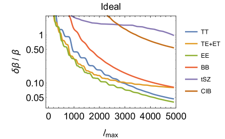
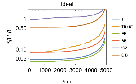
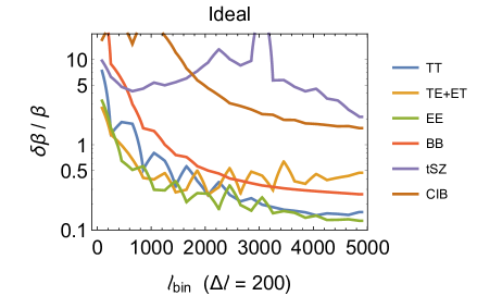
Figure 5: Achievable precision in estimating the velocity through aberration and Doppler effects in an ideal experiment (with $f_{\rm sky}=1$ and limited by cosmic variance only) for different maps. Left: as a function of $\ell_{\rm max}$. Right: as a function of $\ell_{\rm min}$ (with fixed $\ell_{\rm max}=5000$). Bottom: for individual bins with $\Delta\ell=200$. We see that: (i) the first hundred $\ell$s are not important for achieving a high S/N; and (ii) the non-CMB diffuse maps exhibit low precision and are not very useful for measuring $\beta$. Note that for simplicity we have assumed no primordial $B$-modes (our constraints are very weakly sensitive to this choice).

For the tSZ signal, we assume as a fiducial spectrum the one obtained in ref. [Aghanim:2015eva] (slightly extrapolated to higher $\ell$s). For the forecast noise spectrum we use the estimates obtained in ref. [2017arXiv170310456M] using the NILC component separation technique (see figure 14 therein), where it was shown that residual foreground contamination is a large fraction of the total noise. For the CIB signal, we use the spectra obtained in Ref. [Cai2013]; for the noise, we rely on the simulations carried out in Ref. [2016arXiv160907263D]. We also make the conservative assumption that the different channels of the CIB are 100 % correlated. Since different channels pick up different redshifts, effectively the correlation is not going to be total and some extra signal can be obtained from multiple channels; however, since this makes the analysis much more complex (due to the need to have all the covariance matrices) and since the CIB turns out not to be promising for measuring aberration (see Fig. 5), we neglect these corrections.

We computed Eq. (5.16) for the different maps of different experiments. We compared the detection potentials of CORE (see Table 1) with those expected from both Planck and LiteBIRD [2016SPIE.9904E..0XI]. For the Planck specifications, we use the values of the 2015 release, while the LiteBIRD specifications used in this analysis are listed in Table 2.

In Fig. 5 we show the precision that could be reached by an ideal experiment with $f_{\rm sky}=1$ and limited by cosmic variance only. We show the results for: the range $\ell\in[2,\ell_{\rm max}]$; the range $\ell\in[\ell_{\rm min},5000]$; and for individual $\ell$ bins of width $\Delta\ell=200.$ The signal-to-noise ratios in the tSZ and CIB maps are considerably lower than in the CMB maps, which is due to the fact that the spectra are smoother, as explained later. For instance, for $\ell_{\rm max}=4000,$ in the $TT$ and $EE$ maps separately we have ${\rm S/N}>16,$ whereas in tSZ and in CIB we have ${\rm S/N}\simeq 1.$

Channel	Beam	$\Delta T$	$\Delta P$
[GHz]	[arcmin]	[$\mu$K.arcmin]	[$\mu$K.arcmin]
40	108	42.5	60.1
50	86	26	36.8
60	72	20	28.3
68.4	63	15.5	21.9
78	55	12.5	17.7
88.5	49	10	14.1
100	43	12	17.
118.9	36	9.5	13.4
140	31	7.5	10.6
166	26	7	9.9
195	22	5	7.1
234.9	18	6.5	9.2
280	37	10	14.1
337.4	31	10	14.1
402.1	26	19	26.9

Table 2: LiteBIRD specifications used in this analysis.

In Fig. 6 and Table 3 we summarise our forecasts for CORE and compare them with both Planck and LiteBIRD forecasts. These results differ from the ideal case due to the inclusion of instrumental noise, foreground contamination (in the case of tSZ) and $f_{\rm sky}\neq 1.$ In the last panel we also show the total precision by combining all temperature and polarization channels assuming a negligible correlation among them (which was shown in Ref. [Amendola:2010ty] to be a good approximation). Note also that the $TE$ and $ET$ correlation functions were shown to be independent in Ref. [Amendola:2010ty] and both carry the same S/N. So we usually present the combined S/N for $TE+ET$, which is $\sqrt{2}$ times their individual S/N values.

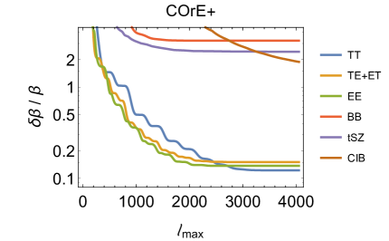
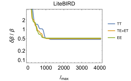
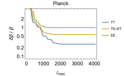
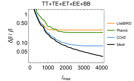
Figure 6: Similar to the left panel of Fig. 5 but for realistic experiments (described in detail in Table 1) and assuming $f_{\rm sky}=0.8.$ In the bottom right panel we compare the total precision after combining all temperature and polarization maps, including also the case of an ideal experiment (no instrumental noise and $f_{\rm sky}=1$).

Experiment	Channel	$\theta_{\rm{FWHM}}$	$\sigma^{T}$	S/N	S/N	S/N	S/N
	[GHz]	[arcmin]	[$\mu$K.arcmin]	$TT$	$TE+ET$	$EE$	Total
Planck	(all)	$\simeq 5.5$	$\simeq 13$	3.8	1.7	1.0	4.3
LiteBIRD	(all)	$\simeq 19$	$\simeq 1.7$	2.0	1.8	1.8	3.3
CORE	60	17.87	7.5	2.1	1.9	1.8	3.4
	70	15.39	7.1	2.5	2.4	2.2	4.1
	80	13.52	6.8	2.8	2.8	2.6	4.8
	90	12.08	5.1	3.5	3.4	3.3	5.9
	100	10.92	5	3.9	3.7	3.7	6.5
	115	9.56	5	4.3	4.2	4.2	7.3
	130	8.51	3.9	5.1	4.9	5.	8.6
	145	7.68	3.6	5.7	5.3	5.5	9.5
	160	7.01	3.7	6.1	5.6	5.8	10.1
	175	6.45	3.6	6.5	5.8	6.1	10.7
	195	5.84	3.5	7.1	6.1	6.5	11.4
	220	5.23	3.8	7.5	6.3	6.7	11.9
	255	4.57	5.6	7.5	5.9	6.2	11.4
	295	3.99	7.4	7.5	5.7	5.8	11.
	340	3.49	11.1	7.	5.1	4.9	9.9
	390	3.06	22	5.8	3.8	3.1	7.6
	450	2.65	45.9	4.5	2.3	1.4	5.3
	520	2.29	116.6	2.9	1.	0.3	3.1
	600	1.98	358.3	1.4	0.3	0.	1.4
	(all)	$\simeq 4.5$	$\simeq 1.4$	8.2	6.6	7.3	12.8
Ideal ($\ell_{\rm max}$ = 2000)	(all)	0	0	5.3	7.1	8.7	12.7
Ideal ($\ell_{\rm max}$ = 3000)	(all)	0	0	10	9.8	14	21
Ideal ($\ell_{\rm max}$ = 4000)	(all)	0	0	16	11.4	19	29
Ideal ($\ell_{\rm max}$ = 5000)	(all)	0	0	22	12.6	26	38

Table 3: Aberration and Doppler effects with CORE. We assume $f_{\rm sky}=0.8$ for all experiments (and $f_{\rm sky}=1$ in the ideal cases) in order to make comparisons simpler. For CORE we assume the 1.2-m telescope configuration, but with extended mission time to match the 1.5-m noise in $\mu$K.arcmin. For CORE and LiteBIRD we assume $\sigma^{P}$ = $\sqrt{2}\sigma^{T}$, while for Planck we use the 2015 values. The combined channel estimates are effective values that best approximate Eq. (5.18) in the $\ell$ range of interest. Note that CORE will have ${\rm S/N}\geq 5$ in 14 different frequency bands. Also, by combining all frequencies, CORE will have similar S/N in $TT$, $TE+ET$ and $EE$.

As a side note, since the estimators for $\left<a_{\ell m}^{X}\leavevmode\nobreak\ a_{(\ell+1)m}^{Y\ast}\right>$ involve a sum over all $\ell$s and $m$s and since $m$ enters through $G_{\ell m}$ only, it is useful to use the following approximations, which are valid to very good accuracy for $\ell\gtrsim 20$ [Notari:2011sb, 2016PhRvD..94d3006N]:

$$\sum_{m}G_{\ell,m}=0.39(2\ell+1)\,;\qquad\sum_{m}\big{[}G_{\ell,m}\big{]}^{2}=0.408^{2}(2\ell+1)\,.$$ (5.19)

Although we did not use these approximations in our results, they yield up to 1 %-level accuracy and by allowing the sum over $m$s to be removed, they significantly simplify the calculation of the estimators.

The achievable precision in $\beta$ through this method depends strongly on the shape of the power spectrum – strongly varying spectra give much lower uncertainties compared to smooth spectra. For instance, for the tSZ and CIB maps, many modes are in the cosmic-variance-limited regime, thus one might think that they would yield a good measurement of $\beta$. However, since their $C_{\ell}$s are smooth functions of $\ell,$ they do not carry much information on the boost. To understand this and gain some insight, we rewrite Eq. (5.9) by approximating $C_{\ell+1}$ as $C_{\ell}+\textrm{d}C_{\ell}/\textrm{d}\ell$ and adding the approximation that $\textrm{d}C_{\ell}/\textrm{d}\ell\ll C_{\ell}$ (note, however, that $\ell\textrm{d}C_{\ell}/\textrm{d}\ell$ could be comparable to $C_{\ell}$ at small scales). We thus find that

$$\sum_{m}\left<a_{\ell m}^{X}\leavevmode\nobreak\ a_{(\ell+1)m}^{Y\ast}\right>=0.39(2\ell+1)\beta\left[(2-2d)C_{\ell}^{XY}-(\ell+d)\frac{\textrm{d}C_{\ell}^{XY}}{\textrm{d}\ell}\right]\,.$$ (5.20)

Assuming the cosmic-variance dominated regime (i.e., ${\mathfrak{C}}^{XX}_{\ell}\simeq C^{XX}_{\ell}$) for $\ell\gtrsim 20$ and putting $X=Y$, we find that

$$\left.\frac{\delta\beta}{\beta}\right|_{XX}\,\simeq\,\frac{1}{0.408\beta}\left[\sum_{\ell}(2\ell+1)\left[(2-2d)-\ell\left(1-\frac{C_{\ell+1}^{XX}}{C_{\ell}^{XX}}\right)\right]^{2}\right]^{-\frac{1}{2}}.$$ (5.21)

For the $TE$ case, the formula is less useful. For the CMB temperature and polarization ($d=1$), only the derivative term survives:

$$\left.\frac{\delta\beta}{\beta}\right|_{XX=TT,EE,BB}\,\simeq\,\frac{1}{0.408\beta}\left[\sum_{\ell}(2\ell+1)\left[\frac{\textrm{d}\ln C_{\ell}^{XX}}{\textrm{d}\ln\ell}\right]^{2}\right]^{-\frac{1}{2}}.$$ (5.22)

Note that for the CIB the precision is smaller than for the CMB temperature and polarization, not only because the spectra are smoother, but also because there is a partial cancellation between the two terms in the summand of Eq. (5.21).

In this analysis we relied only on the diffuse background components of the measured maps. Aberration and Doppler effects can in principle also be detected using point sources, since the boosting effects will change both their number counts, angular distribution, and redshift. For the upcoming CMB experiments, however, the number density of point sources is probably insufficient for a significant signal, since one needs more than about $10^{6}$ objects to have a detection at greater than $1\,\sigma$ [Yoon:2015lta].

6 Differential approach to CMB spectral distortions and the CIB

Using the complete description of the Compton-Getting effect [1970PSS1825F] we compute full-sky maps of the expected effect at desired frequency. We start discussing the frequency dependence of the dipole spectrum [DaneseDeZotti1981, Balashev2015] and then extend the analysis beyond the dipole.

6.1 The CMB dipole

The dipole amplitude is directly proportional to the first derivative of the photon occupation number, $\eta(\nu)$, which is related to the thermodynamic temperature, $T_{\rm therm}(\nu)$, i.e., to the temperature of the blackbody having the same $\eta(\nu)$ at the frequency $\nu$, by

$$T_{\rm therm}={h\nu\over k_{\rm B}\ln(1+1/\eta(\nu))}.$$ (6.1)

The difference in $T_{\rm therm}$ measured in the direction of motion and in the perpendicular direction is given by [DaneseDeZotti1981]:

$$\Delta T_{\rm therm}={h\nu\over k}\left\{{1\over\ln\left[1+1/\eta(\nu)\right]}-{1\over\ln\left[1+1/\eta(\nu(1+\beta))\right]}\right\}\,,$$ (6.2)

which, to first order, can be approximated by:

$$\Delta T_{\rm therm}\simeq-{x\beta T_{0}\over(1+\eta)\ln^{2}(1+1/\eta)}{d\ln\eta\over d\ln x},$$ (6.3)

where $x\equiv h\nu/kT_{0}$ is the dimensionless frequency.

In Fig. 7 we show the dipole spectrum derived for two well-defined deviations from the Planck distribution, namely the BE and Comptonization distortions induced by unavoidable energy injections in the radiation field occurring at different cosmic times, early and late, respectively. We briefly discuss below their basic properties and the signal levels expected from different processes.

A BE-like distorted spectrum is produced by two distinct processes. Firstly there is the dissipation of primordial perturbations at small scales [1994ApJ...430L...5H, chlubasunyaev2012], which generates a positive chemical potential. Secondly we have Bose condensation of CMB photons by colder electrons, as a consequence of the faster decrease of the matter temperature relative to the radiation temperature in an expanding Universe, which generates a negative chemical potential [2012MNRAS.419.1294C, sunyaevkhatri2013].

The photon occupation number of the BE spectrum is given by [1970Ap&SS...7...20S]

$$\eta_{\rm BE}={1\over e^{x_{\rm e}+\mu}-1},$$ (6.4)

where $\mu$ is the chemical potential that quantifies the fractional energy, $\Delta\epsilon/\varepsilon_{\rm i}$, exchanged in the plasma during the interaction, $x_{\rm e}=x/\phi(z)$, $\phi(z)=T_{\rm e}(z)/T_{\rm CMB}(z)$, with $T_{\rm e}(z)$ being the electron temperature. For a BE spectrum, $\phi=\phi_{\rm BE}(\mu)$. The dimensionless frequency $x$ is redshift invariant, since in an expanding Universe both $T_{\rm CMB}$ and the physical frequency $\nu$ scale as $(1+z)$. For small distortions, $\mu\simeq 1.4\Delta\epsilon/\varepsilon_{\rm i}$ and $\phi_{\rm BE}\simeq(1-1.11\mu)^{-1/4}$. The current FIRAS 95 % CL upper limit is $|\mu_{0}|<9\times 10^{-5}$ [1996ApJ...473..576F], where $\mu_{0}$ is the value of $\mu$ at the redshift $z_{1}$ corresponding to the end of the kinetic equilibrium era. At earlier times $\mu$ can be significantly higher, and the ultimate limits on $\Delta\epsilon/\varepsilon_{\rm i}$ before the thermalization redshift (when any distortion can be erased) comes from cosmological nucleosynthesis.

These two kinds of distortions are characterised by a $|\mu_{0}|$ value in the range, respectively, $\sim 10^{-9}$–$10^{-7}$ (and in particular $\simeq 2.52\times 10^{-8}$ for a primordial scalar perturbation spectral index $n_{\rm s}=0.96$, without running), and $\simeq 3\times 10^{-9}$. Since very small scales that are not explored by current CMB anisotropy data are relevant in this context, a broad set of primordial spectral indices needs to be explored. A wider range of chemical potentials is found by [chlubaal12], allowing also for variations in the amplitude of primordial perturbations at very small scales, as motivated by some inflation models.

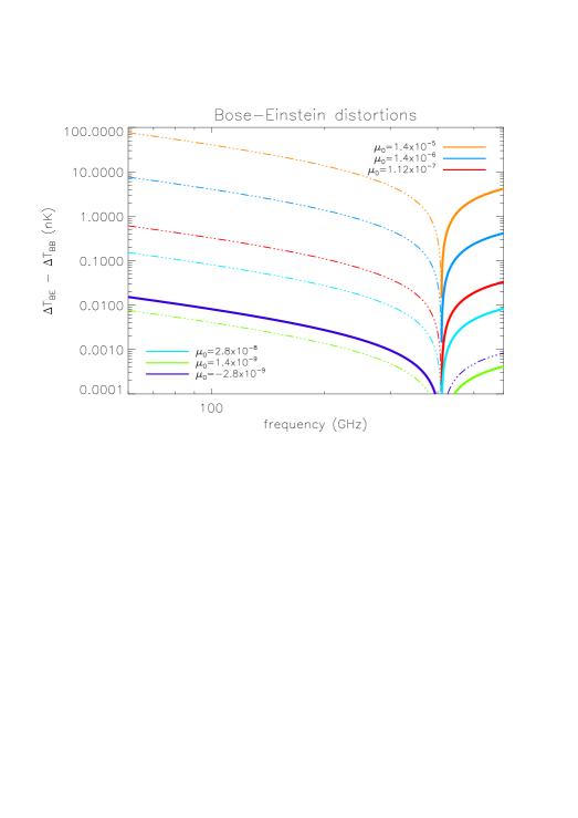
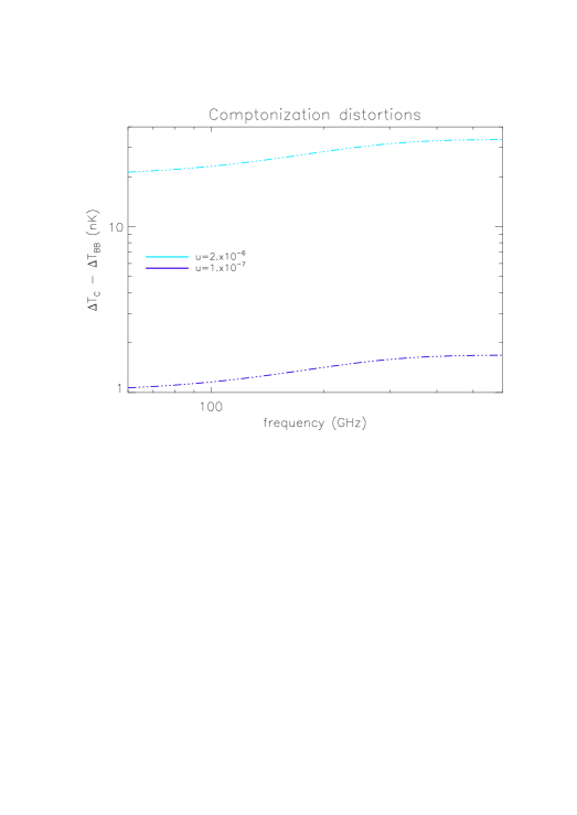
Figure 7: Spectrum of dipole (in equivalent thermodynamic, or CMB, temperature) expressed as the difference between that produced by a distorted spectrum and that corresponding to the blackbody at the current temperature $T_{0}$. Thick solid lines (or thin three dots-dashes) correspond to positive (or negative) values. Left: the case of BE distortions for $\mu_{0}=-2.8\times 10^{-9}$ (representative of adiabatic cooling; green dots, note the opposite signs with respect to the cases with positive $\mu_{0}$), $\mu_{0}=1.4\times 10^{-5}$, $1.4\times 10^{-6}$ (representative of improvements with respect to FIRAS upper limits), $\mu_{0}=1.12\times 10^{-7}$, $2.8\times 10^{-8}$, and $1.4\times 10^{-9}$ (representative of primordial adiabatic perturbation dissipation). Right: the case of Comptonization distortions for $u=2\times 10^{-6}$ (upper curves) and $u=10^{-7}$ (lower curves), representative of imprints by astrophysical or minimal reionization models, respectively.

Cosmological reionization associated with the early stages of structure and star formation is an additional source of photon and energy production. This mechanism induces electron heating that is responsible for Comptonization distortions [1972JETP...35..643Z]. The characteristic parameter for describing this effect is

$$u(t)=\int_{t_{\rm i}}^{t}[(\phi-\phi_{\rm i})/\phi](k_{\rm B}T_{\rm e}/m_{\rm e}c^{2})n_{\rm e}\sigma_{\rm T}cdt\,.$$ (6.5)

In the case of small energy injections and integrating over the relevant epochs then $u\simeq(1/4)\Delta\varepsilon/\varepsilon_{\rm i}$. In Eq. (6.5), $\phi_{\rm i}=\phi(z_{\rm i})=(1+\Delta\epsilon/\varepsilon_{\rm i})^{-1/4}\simeq 1-u$ is the ratio between the equilibrium matter temperature and the radiation temperature evaluated at the beginning of the heating process (i.e., at $z_{\rm i}$). The distorted spectrum is then

$$\eta_{\rm C}\simeq\eta_{\rm i}+u{x/\phi_{\rm i}{\rm exp}(x/\phi_{\rm i})\over[{\rm exp}(x/\phi_{\rm i})-1]^{2}}\left({x/\phi_{\rm i}\over{\rm tanh}(x/2\phi_{\rm i})-4}\right),$$ (6.6)

where $\eta_{\rm i}$ is the initial photon occupation number (before the energy injection).

Typically, reionization induces Comptonization distortions with minimal values $u\simeq 10^{-7}$ [buriganaetal08]. In addition to this, the variety of energy injections expected in astrophysical reionization models, including: energy produced by nuclear reactions in stars and/or by nuclear activity that mechanically heats the intergalactic medium (IGM); super-winds from supernova explosions and active galactic nuclei; IGM heating by quasar radiative energy; and shocks associated with structure formation. Together these induce much larger values of $u$ ($\simeq\hbox{several}\times 10^{-6}$) [2000PhRvD..61l3001R, 2015PhRvL.115z1301H], i.e., not much below the current FIRAS 95 % CL upper limit of $|u|<1.5\times 10^{-5}$ [1996ApJ...473..576F]. Free-free distortions associated with reionization [2014MNRAS.437.2507T] are instead more relevant at the lowest frequencies (below $10\,$GHz), and thus we do not consider them in this paper.

We could also consider the possible presence of unconventional heating sources. Decaying and annihilating particles during the pre-recombination epoch may affect the CMB spectrum, with the exact distorted shape depending on the process timescale and, in some cases, being different from the one produced by energy release. This is especially interesting for decaying particles with lifetimes $t_{X}\simeq$ few$\times 10^{8}$–$10^{11}$ sec [1993PhRvL..70.2661H, daneseburigana94, 2013MNRAS.436.2232C]. Superconducting cosmic strings would also produce copious electromagnetic radiation, creating CMB spectral distortion shapes [ostrikerthompson87] that would be distinguishable with high accuracy measurements. Evaporating primordial black holes provide another possible source of energy injection, with the shape of the resulting distortion depending on the black hole mass function [carretal2010]. CMB spectral distortion measurements could also be used to constrain the spin of non-evaporating black holes [paniloeb2013]. The CMB spectrum could additionally set constraints on the power spectrum of small-scale magnetic fields [jedamziketal2000], the decay of vacuum energy density [BartlettSilk1990], axions [ejllidolgov2014], and other new physical processes.

6.2 The CIB dipole

Multi-frequency measurements of the dipole spectrum will allow us to constrain the CIB intensity spectrum [DaneseDeZotti1981, Balashev2015]. The spectral shape of the CIB is hard to determine directly because it requires absolute intensity measurements, which are also compromised by Galactic and other foregrounds. Although the dipole amplitude is about $10^{-3}$ of the monopole, its spatial form is already known and hence this indirect route may provide the most robust measurements of the CIB in the future.

Fig. 8 shows the CIB dipole spectrum computed according to Eq. (6.2), using the analytic representation of the CIB spectrum (observed at present time) given in Ref. [Fixsen:1998kq]:

$$\eta_{\rm CIB}={c^{2}\over 2h\nu^{3}}I_{\rm CIB}(\nu)=I_{0}\left({k_{\rm B}T_{\rm CIB}\over h\nu_{0}}\right)^{k_{F}}{x^{k_{\rm F}}_{\rm CIB}\over\exp(x_{\rm CIB})-1}\,,$$ (6.7)

where $T_{\rm CIB}=(18.5\pm 1.2)\,$K, $x_{\rm CIB}=h\nu/k_{\rm B}T_{\rm CIB}=7.78(\nu/\nu_{0})$, $\nu_{0}\simeq 3\times 10^{12}\,$Hz and $k_{\rm F}=0.64\pm 0.12$. Here $I_{0}$ sets the CIB spectrum amplitude, its best-fit value being $1.3\times 10^{-5}$ [Fixsen:1998kq]. On the other hand, the uncertainty of the CIB amplitude is currently quite high, with $I_{0}$ only known to a 1 $\sigma$ accuracy of about 30 %.

The CIB dipole amplitude, in terms of thermodynamic temperature, increases rapidly with frequency, reaching $257\,\mu$K (or $652\,\hbox{Jy}\,\hbox{sr}^{-1}$) at 600 GHz and $420\,\mu$K (or $1306\,\hbox{Jy}\,\hbox{sr}^{-1}$) at 800 GHz. The measurement of the CIB dipole amplitude will be dependent on systematic effects from the foreground Galaxy subtraction, which has a similar spectrum to the CIB [2011ApJ...734...61F]. Although the calibration of the dipole signal at different frequencies is not trivial (since the orbital part of the dipole will be used for calibration), the Planck experience is that with sufficient care the limitation is removal of the Galactic signals, not calibration uncertainty. Hence the CIB dipole should be clearly detectable by CORE in its highest frequency bands. Such a detection will provide important constraints on the CIB intensity; its amplitude uncertainty constitutes a major current limitation in our understanding of the dust-obscured star-formation phase of galaxy evolution.

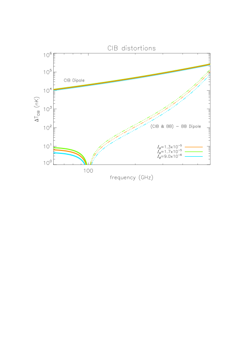
Figure 8: Expected behaviour of the dipole spectrum. The upper lines show the spectrum of the (pure) CIB dipole, while the lower lines show the spectrum coming from the dipole pattern computed from the CIB distribution function added to the blackbody (at temperature $T_{0}$) distribution function, minus the dipole pattern computed by the blackbody distribution function. Thick solid lines (or thin three dots-dashes) correspond to positive (or negative) values. The analytic representation of the CIB spectrum by [Fixsen:1998kq] is adopted here, considering the best-fit amplitude and the range of $\pm 1\,\sigma$.

Figure 9: Top row: maps of the dipole, quadrupole and octupole computed assuming a CMB blackbody spectrum at the current temperature $T_{0}$, for reference. In all other cases we show the maps of the dipole (second row), quadrupole (third row), and octupole (bottom row) at three different frequencies (namely 60, 145, and 600 GHz, from left to right), in terms of the difference between the pattern computed for a BE distortion with $\mu_{0}=1.5\times 10^{-5}$ and that computed for a blackbody at the present-day temperature $T_{0}$.

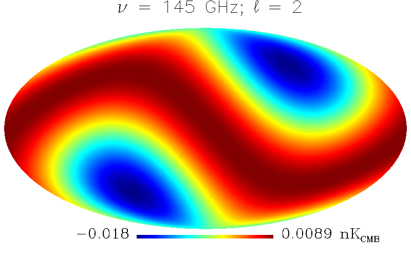
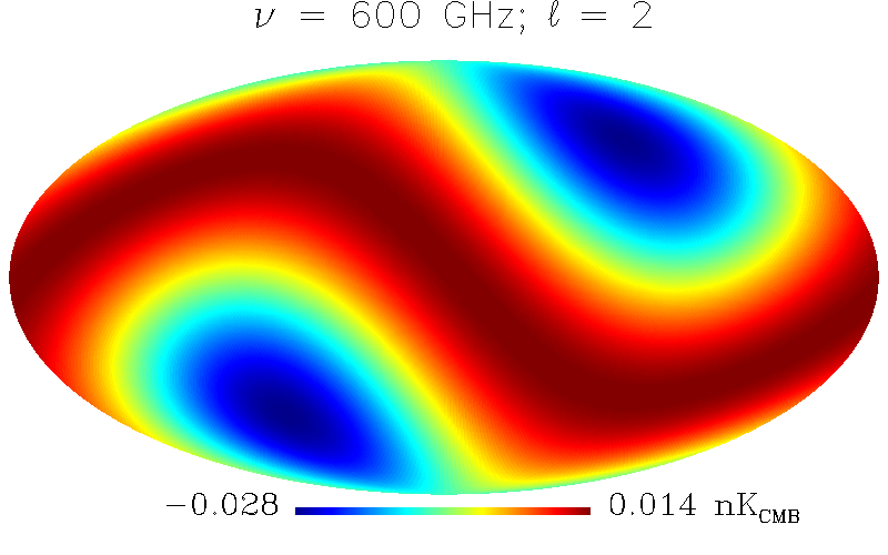
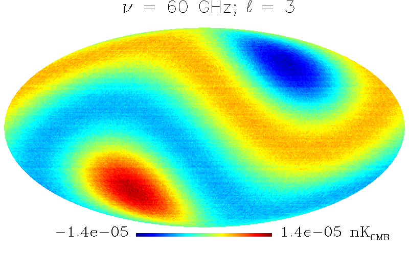
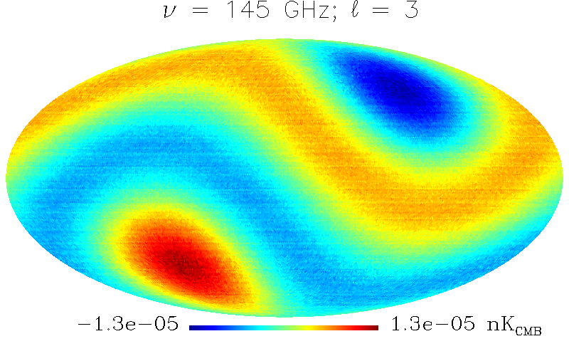
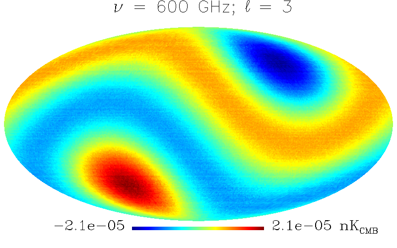
Figure 10: The same as in Fig. 9, but for the case of a Comptonization distortion with $u=2\times 10^{-6}$.

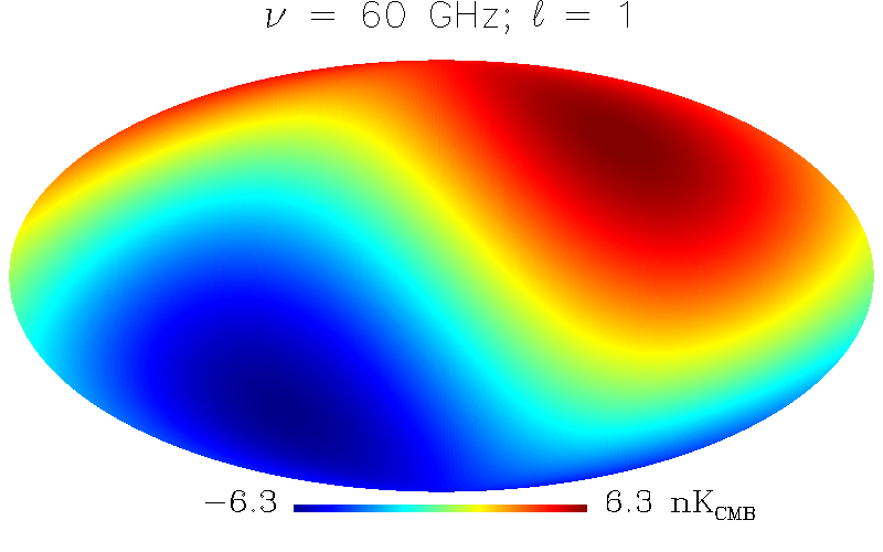
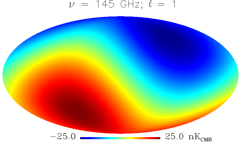
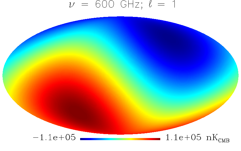
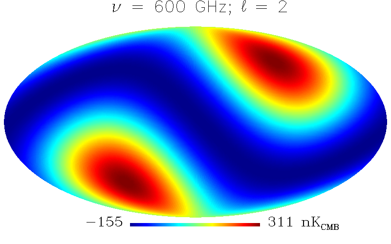
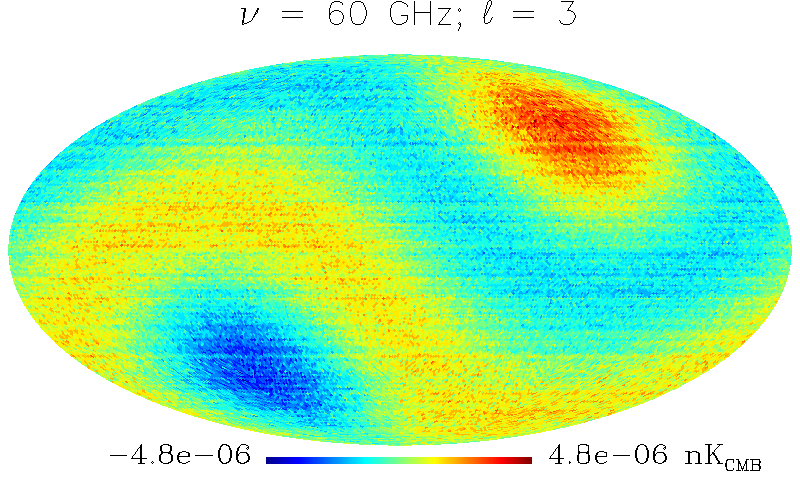
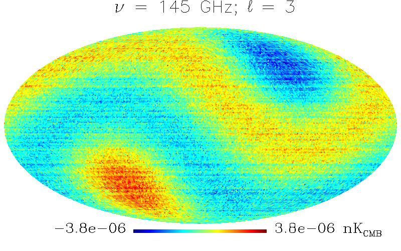
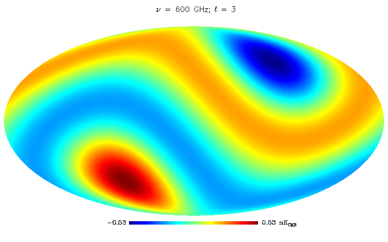
Figure 11: The same as in Fig. 9, but for the case of the CIB with amplitude set at the best-fit value found by FIRAS. More precisely, we display the temperature pattern of the CIB distribution function added to the blackbody one, minus the temperature pattern coming from the blackbody.

6.3 Beyond the dipole

A generalization of the considerations of the previous section allows us to evaluate the effect of peculiar velocity on the whole sky. To achieve this, we generate maps and, using the Lorentz-invariance of the distribution function, we can include all orders of the effect, coupling them with the geometrical properties induced at low multipoles. To compute the maps at each multipole $\ell\geq 1$, we first derive the maps at all angular scales, both for the distorted spectra and for the blackbody at the current temperature $T_{0}$. From the dipole direction found in the Planck (HFI+LFI combined) 2015 release and defining the motion vector of the observer, we produce the maps in a pixelization scheme at a given observational frequency $\nu$ by computing the photon distribution function, $\eta^{\rm BBdist}$, for each considered type of spectrum at a frequency given by the observational frequency $\nu$ but multiplied by the product $(1-\hat{n}\cdot\vec{\beta})/(1-\vec{\beta}^{2})^{1/2}$ to account for all the possible sky directions with respect to the observer peculiar velocity. Here the notation ‘BBdist’ stands for BB, CIB, BE, or Comptonization (C). Hence, the map of the observed signal in terms of thermodynamic temperature is given by generalising Eq. (6.1):

$$T_{\rm therm}^{\rm BB/dist}(\nu,{\hat{n}},\vec{\beta})=\frac{xT_{0}}{{\rm{log}}(1/(\eta(\nu,{\hat{n}},\vec{\beta}))^{\rm BB/dist}+1)}\,,$$ (6.8)

where $\eta(\nu,{\hat{n}},\vec{\beta})=\eta(\nu^{\prime})$ with $\nu^{\prime}=\nu(1-{\hat{n}}\cdot\vec{\beta})/(1-\vec{\beta}^{2})^{1/2}$.

We adopt the HEALPix pixelization scheme to discretise the sky at the desired resolution. We decompose the maps into spherical harmonics and then regenerate them considering the $a_{lm}$ only up to a desired multipole $\ell_{\rm{max}}$. We start setting $\ell_{\rm{max}}=5$ and then iterate the process with a decreasing $\ell_{\rm{max}}$. We produce maps containing the power at a single multipole by taking the difference of the map at $\ell_{\rm{max}}$ from the map at $\ell_{\rm{max}-1}$. We then compute the difference of maps having specific spectral distortions from the purely blackbody maps. As seen in Figs. 9–11, the expected signal is important for the dipole, can be considerable for the quadrupole and, depending on the distortion parameters, still not negligible for the octupole (although this will depend on the amplitude relative to experimental noise levels, as we discuss below). For higher-order multipoles, the signal is essentially negligible.

Note that the maps present a clear and obvious symmetry with respect to the axis of the observer’s peculiar velocity. This is simply due to the angular dependence in Eq. (6.8). For coordinates in which the positive $z$-axis is aligned with the dipole, the only angular dependence comes from $\hat{n}\cdot\vec{\beta}\equiv\beta\cos{\theta_{\rm d}}$. In terms of the spherical harmonic expansion, this implies that higher-order multipoles will appear as polynomial functions of $\cos{\theta_{\rm d}}$, with different frequency-dependent factors depending on the specific type of spectral distortion being considered.

In the above considerations we assumed that each multipole pattern can be isolated from that of the other multipoles. In reality, a certain leakage is expected (particularly between adjacent multipoles), especially as a result of masking for foregrounds. The sources of astrophysical emission are highly complex, and their geometrical properties mix with their frequency behaviour. Furthermore, in real data analysis, there is an interplay between the determination of the calibration and zero levels of the maps, and this issue is even more critical when data in different frequency domains are used to improve the component-separation process. The analysis of these aspects is outside the scope of the present paper, but deserves further investigation.

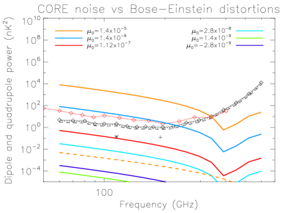
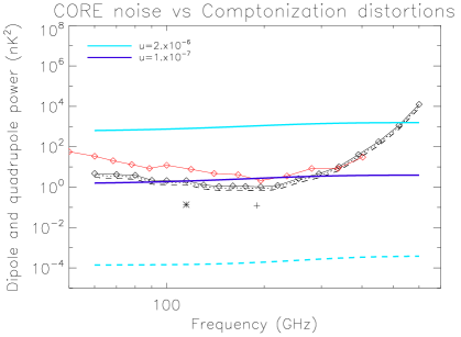
Figure 12: Angular power spectrum of the dipole map, derived from the difference between distorted spectra and the current blackbody spectrum versus CORE sensitivity. The CORE white noise power spectrum (independent of multipole, shown as the black upper solid curve and with diamonds for different frequency channels) and its rms uncertainty (for $\ell=1$, using dots, and for $\ell=2$, using dashes) are plotted in black. The cross (asterisk) displays aggregated CORE noise from all channels (up to 220 GHz). We shown also for comparison the LiteBIRD white noise power spectrum (red solid curve and diamonds for different frequency channels). Left: BE distortions for $\mu_{0}=-2.8\times 10^{-9}$ (representative of adiabatic cooling), $\mu_{0}=1.4\times 10^{-5}$, $1.4\times 10^{-6}$ (representative of improvements with respect to FIRAS upper limits), $\mu_{0}=1.12\times 10^{-7}$, $2.8\times 10^{-8}$, and $1.4\times 10^{-9}$ (representative of primordial adiabatic perturbation dissipation). For $\mu_{0}=1.4\times 10^{-5}$ we show also the angular power spectrum of the quadrupole map. Right: Comptonization distortions for $u=2\times 10^{-6}$ (upper solid curve for the dipole map and bottom dashed curve for the quadrupole map) and $u=10^{-7}$ (lower solid curve for the dipole map), representative of imprints by astrophysical and minimal reionization models, respectively.

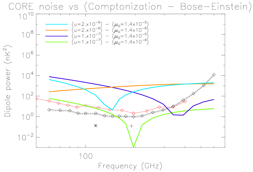
Figure 13: The same as in Fig. 12, but comparing the two above cases of Comptonization distortions with the two above cases of BE distortions with the largest values of $\mu_{0}$.

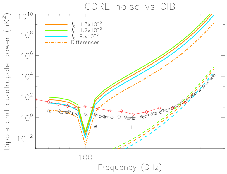
Figure 14: The same as in Fig. 12, but for the CIB (assuming the model from [Fixsen:1998kq]). Also shown is the quadrupole signal (dashes). The different values of $I_{0}$ in Eq. (6.8) are the best-fit value and deviations by $\pm 1\,\sigma$.

6.4 Detectability

Here we discuss the detectability of the dipolar and quadrupolar signals introduced in Sects. 6.1–6.3. To this end we compare the dipole signal with the noise dipole as a function of frequency. Note that since the prediction includes the specific angular dependence of the dipole, there is no cosmic-variance related component in the noise. The noise for each frequency is determined by Table 1, assuming full-sky coverage for simplicity.

In Fig. 12 we show the dipole signal for BE and Comptonization distortions (left and right, respectively), defined as the temperature dipole coming from Eq. (6.8) subtracted from the CMB dipole (shown as coloured lines). In black we show the CORE noise as a function of frequency. For BE distortions, the signal is clearly above the CORE noise up to about 200 GHz for $\mu_{0}\,\lower 2.0pt\hbox{${>\atop\hbox{\raise 4.0pt\hbox{$\sim$}}}$}\,10^{-6}$ and comparable or slightly above the aggregated noise below about 100 GHz for $\mu_{0}\,\lower 2.0pt\hbox{${>\atop\hbox{\raise 4.0pt\hbox{$\sim$}}}$}\,10^{-7}$, while for Comptonization distortions, the signal is clearly above the noise up to around 500 GHz for $u\,\lower 2.0pt\hbox{${>\atop\hbox{\raise 4.0pt\hbox{$\sim$}}}$}\,2\times 10^{-6}$ and comparable to or above the noise between approximately 100 GHz and 300 GHz for $u\,\lower 2.0pt\hbox{${>\atop\hbox{\raise 4.0pt\hbox{$\sim$}}}$}\,10^{-7}$. The analogous analysis for the quadrupole (shown for simplicity only for the largest values of $\mu_{0}$ and $u$) shows that, for CORE sensitivity, noise dominates at any frequency for CMB spectral distortion parameters compatible with FIRAS limits, thus experiments beyond CORE are needed to use the quadrupole pattern to infer constraints on CMB spectral distortions. In Fig. 14 we show the dipole signal of the difference between Comptonization and BE distortion maps. In Fig. 14 we show the size of the dipole signal (the quadrupole is shown as dashed curves) for the CIB (where we have removed the CMB dipole) compared to noise. The signal is always above the noise except at about 100 GHz. Due to the large uncertainty in the amplitude of the CIB spectra ($I_{0}$), we show also deviations of $\pm 1\,\sigma$ from the best-fit value of $1.3\times 10^{-5}$ (as well as their difference from the best fit). The signal is orders of magnitude above the noise at high frequencies and moreover, the quadrupole is above the noise at frequencies greater than about 400 GHz, although it is always much smaller than the dipole (since it is suppressed by an extra factor of $\beta$).

Comparing Fig. 14 with Fig. 12, it is evident that the dipole power expected from the CIB is above those predicted for CMB spectral distortions at $\nu\,\lower 2.0pt\hbox{${>\atop\hbox{\raise 4.0pt\hbox{$\sim$}}}$}\,200$ GHz for the classes of processes and parameter values discussed here. Since the dependence of the quoted power on the CMB spectral distortion parameter is quadratic, the above statement does not hold for larger CMB distortions, even just below the FIRAS limits. Although they are not predicted by standard scenarios, they may be generated by unconventional dissipation processes, such those discussed at the end of Sect. 6.1, according to their characteristic parameters.

We computed for comparison the power spectrum sensitivity of LiteBIRD (see Table 2): it is similar to that of CORE around 300 GHz and significantly worse at $\nu\,\lower 2.0pt\hbox{${<\atop\hbox{\raise 4.0pt\hbox{$\sim$}}}$}\,150$ GHz, a range suitable in particular for BE distortions. As discussed in Sects. 2 and 4, resolution is important to achieve the sky sampling necessary for ultra-accurate dipole analysis, thus adopting a resolution changing from a range of $\simeq 2$–18 arcmin to a range of $\simeq 0.5^{\circ}$–$1.5^{\circ}$ is certainly critical. Furthermore, the number of frequency channels is relevant, in particular (see next section) when one compares between pairs of frequencies, the number of which scales approximately as the square of the number of frequency channels. In addition, a large number of frequency channels and especially the joint analysis of frequencies around 300 GHz and above 400 GHz (not foreseen in LiteBIRD) is crucial for separating the various types of signals, and, in particular, to accurately control the contamination by Galactic dust emission.

The analysis carried out here will be extended to include all frequency information in the following section. This will also include a discussion of the impact of residual foregrounds.

7 Simulation results for CMB spectral distortions and CIB intensity

In order to quantify the ideal CORE sensitivity to measure spectral distortion parameters and the CIB amplitude, we carried out some detailed simulations. The idea here is to simulate the sky signal assuming a certain model and to quantify the accuracy level at which (in the presence of noise and of potential residuals) we can recover the key input parameters. We consider twelve reference cases, physically or observationally motivated, based on considerations and works quoted in Sect. 6.2 (cases 2–4) and Sect. 6.1 (cases 8–12), namely:

(1) a (reference) blackbody spectrum defined by $T_{0}$;
(2) a CIB spectrum at the FIRAS best-fit amplitude;
(3) a CIB spectrum at the FIRAS best-fit amplitude plus $1\,\sigma$ error;
(4) a CIB spectrum at the FIRAS best-fit amplitude minus $1\,\sigma$ error;
(5) a BE spectrum with $\mu_{0}=1.12\times 10^{-7}$, representative of a distortion induced by damping of primordial adiabatic perturbations in the case of relatively high power at small scales;
(6) a BE spectrum with $\mu_{0}=1.4\times 10^{-5}$, a value 6.4 times smaller than the FIRAS $95\,\%$ upper limits;
(7) a BE spectrum with $\mu_{0}=1.4\times 10^{-6}$, a value 64 times smaller than the FIRAS $95\,\%$ upper limits;
(8) a BE spectrum with $\mu_{0}=1.4\times 10^{-9}$, representative of the typical minimal distortion induced by the damping of primordial adiabatic perturbations;
(9) a BE spectrum with $\mu_{0}=2.8\times 10^{-8}$, representative of the typical distortion induced by damping of primordial adiabatic perturbations;
(10) a BE spectrum with $\mu_{0}=-2.8\times 10^{-9}$, representative of the typical distortion induced by BE condensation (adiabatic cooling);
(11) a Comptonised spectrum with $u=10^{-7}$, representative of minimal reionization models;
(12) a Comptonised spectrum with $u=2\times 10^{-6}$, representative of typical astrophysical reionization models.

For each model listed we generate both an ideal sky (the “prediction”) and a sky with noise realizations (“simulated data”) according to the sensitivity of CORE (see Table 1), at each of its 19 frequency channels. For a suitable number of cases we repeated the analysis working with maps simply containing only the dipole term and verified that the major contribution to the significance comes from the dipole, i.e., the quadrupole (the only other possibly relevant term) contributes almost negligibly, in agreement with Sect. 6.4. For the sake of simplicity our noise realizations assume Gaussian white noise. Our simulation set consists of 10 realizations for each of the 19 CORE frequencies (giving 190 independent noise realizations). These are generated at $N_{\rm side}=64$ (roughly $1^{\circ}$ resolution). We will also consider the inclusion of certain systematics in the following subsections. We then compare each theoretical prediction with all maps of our simulated data. We calculate $\Delta\chi^{2}$ for each combination, summarised in a $12\times 12$ matrix, quantifying the significance level at which each model can be potentially detected or ruled out. We report our results in terms of $\sqrt{|\Delta\chi^{2}|}\;{\rm sign}(\Delta\chi^{2})$, which directly gives the significance in terms of $\sigma$ levels, since we only consider a single parameter at a time.

We perform the $\sqrt{\Delta\chi^{2}}$ analysis for three different approaches:

1. using each of the 19 frequency channels, assuming they are independent;

2. using the 171 ($19\times 18/2$) combinations coming from the differences of the maps from pairs of frequency bands;

3. combining cases (a) and (b) together.

When differences of maps from pairs of frequency bands are included in the analysis, in the corresponding contributions to the $\chi^{2}$ the variance comes from the sum of the variances at the two considered frequencies.

Approach (a) essentially compares the amplitude of dipole of a distorted spectrum with that of the blackbody, being so sensitive to the overall difference between the two cases, while approach (b) compares the dipole signal at different frequencies for each type of spectrum, being so sensitive to its slope.

7.1 Ideal case: perfect calibration and foreground subtraction

$\sigma$ level Current FIRAS CIB amplitude $(\Delta\varepsilon/\varepsilon_{\rm i})_{z_{1}}$ $(\Delta\varepsilon/\varepsilon_{\rm i})_{\rm late}$ significance blackbody (units $10^{-5}$) $8\times 10^{-8}$ $10^{-5}$ $10^{-6}$ $10^{-9}$ $2\times 10^{-8}$ $-2\times 10^{-9}$ $4\times 10^{-7}$ $8\times 10^{-6}$ $I_{0}^{\rm bf}$ $+1\,\sigma$ $-1\,\sigma$ $\mu_{0}$ $u$ $1.3$ $1.7$ $0.9$ $1.12\times 10^{-7}$ $1.4\times 10^{-5}$ $1.4\times 10^{-6}$ $1.4\times 10^{-9}$ $2.8\times 10^{-8}$ $-2.8\times 10^{-9}$ $10^{-7}$ $2\times 10^{-6}$ Case (1) (2) (3) (4) (5) (6) (7) (8) (9) (10) (11) (12) $(1)$ $0$ $3650$ $4740$ $2540$ $1.63$ $175.$ $17.9$ $0.0998$ $0.532$ $-0.137$ $7.95$ $154.$ $(2)$ $3650$ $0$ $1100$ $1110$ $3650$ $3640$ $3650$ $3650$ $3650$ $3650$ $3650$ $3620$ $(3)$ $4740$ $1100$ $0$ $2210$ $4740$ $4740$ $4740$ $4740$ $4740$ $4740$ $4740$ $4710$ $(4)$ $2540$ $1110$ $2200$ $0$ $2540$ $2540$ $2540$ $2540$ $2540$ $2540$ $2540$ $2510$ $(5)$ $0.403$ $3650$ $4740$ $2540$ $0$ $174.$ $16.5$ $0.384$ $-0.111$ $0.445$ $6.83$ $153.$ $(6)$ $174.$ $3640$ $4740$ $2540$ $173.$ $0$ $157.$ $174.$ $174.$ $174.$ $168.$ $108.$ $(7)$ $17.0$ $3650$ $4740$ $2540$ $15.6$ $158.$ $0$ $17.0$ $16.6$ $17.0$ $11.8$ $140.$ $(8)$ $-0.0975$ $3650$ $4740$ $2540$ $1.62$ $175.$ $17.9$ $0$ $0.514$ $-0.165$ $7.93$ $154.$ $(9)$ $-0.346$ $3650$ $4740$ $2540$ $1.28$ $175.$ $17.6$ $-0.342$ $0$ $-0.352$ $7.66$ $153.$ $(10)$ $0.142$ $3650$ $4740$ $2540$ $1.67$ $175.$ $17.9$ $0.176$ $0.567$ $0$ $7.98$ $154.$ $(11)$ $7.25$ $3650$ $4740$ $2540$ $6.22$ $169.$ $12.8$ $7.23$ $6.98$ $7.27$ $0$ $146.$ $(12)$ $153.$ $3620$ $4710$ $2510$ $152.$ $108.$ $140.$ $153.$ $153.$ $153.$ $145.$ $0$

Table 4: Average values of $\sqrt{|\Delta\chi^{2}|}\;{\rm sign}(\Delta\chi^{2})$ from a Monte Carlo simulation at $N_{\rm side}=64$, full-sky coverage, adopting perfect foreground subtraction and calibration, and considering each of the 19 frequency channels.

$\sigma$ level Current FIRAS CIB amplitude $(\Delta\varepsilon/\varepsilon_{\rm i})_{z_{1}}$ $(\Delta\varepsilon/\varepsilon_{\rm i})_{\rm late}$ significance blackbody (units $10^{-5}$) $8\times 10^{-8}$ $10^{-5}$ $10^{-6}$ $10^{-9}$ $2\times 10^{-8}$ $-2\times 10^{-9}$ $4\times 10^{-7}$ $8\times 10^{-6}$ $I_{0}^{\rm bf}$ $+1\,\sigma$ $-1\,\sigma$ $\mu_{0}$ $u$ $1.3$ $1.7$ $0.9$ $1.12\times 10^{-7}$ $1.4\times 10^{-5}$ $1.4\times 10^{-6}$ $1.4\times 10^{-9}$ $2.8\times 10^{-8}$ $-2.8\times 10^{-9}$ $10^{-7}$ $2\times 10^{-6}$ Case (1) (2) (3) (4) (5) (6) (7) (8) (9) (10) (11) (12) $(1)$ $0$ $14000$ $18200$ $9740$ $1.96$ $271.$ $27.8$ $0.124$ $0.666$ $-0.170$ $-0.229$ $43.7$ $(2)$ $14000$ $0$ $4180$ $4240$ $14000$ $14100$ $14000$ $14000$ $14000$ $14000$ $14000$ $14000$ $(3)$ $18200$ $4190$ $0$ $8430$ $18200$ $18200$ $18200$ $18200$ $18200$ $18200$ $18200$ $18200$ $(4)$ $9740$ $4240$ $8420$ $0$ $9740$ $9810$ $9750$ $9740$ $9740$ $9740$ $9740$ $9730$ $(5)$ $0.0596$ $14000$ $18200$ $9740$ $0$ $269.$ $25.6$ $0.0456$ $-0.249$ $0.0910$ $1.44$ $45.7$ $(6)$ $269.$ $14000$ $18200$ $9810$ $267.$ $0$ $242.$ $269.$ $269.$ $269.$ $271.$ $312.$ $(7)$ $26.0$ $14000$ $18200$ $9750$ $23.8$ $244.$ $0$ $26.0$ $25.4$ $26.1$ $28.1$ $69.6$ $(8)$ $-0.122$ $14000$ $18200$ $9740$ $1.93$ $271.$ $27.8$ $0$ $0.644$ $-0.205$ $-0.209$ $43.7$ $(9)$ $-0.386$ $14000$ $18200$ $9740$ $1.51$ $271.$ $27.2$ $-0.384$ $0$ $-0.391$ $0.228$ $44.2$ $(10)$ $0.178$ $14000$ $18200$ $9740$ $2.00$ $271.$ $27.9$ $0.220$ $0.708$ $0$ $-0.267$ $43.6$ $(11)$ $2.66$ $14000$ $18200$ $9740$ $4.69$ $273.$ $29.9$ $2.68$ $3.11$ $2.62$ $0$ $41.4$ $(12)$ $46.4$ $14000$ $18200$ $9730$ $48.4$ $314.$ $72.0$ $46.4$ $46.9$ $46.4$ $44.1$ $0$

Table 5: The same as in Table 4, but considering all 171 independent combinations of pairs of different frequency channels.

$\sigma$ level Current FIRAS CIB amplitude $(\Delta\varepsilon/\varepsilon_{\rm i})_{z_{1}}$ $(\Delta\varepsilon/\varepsilon_{\rm i})_{\rm late}$ significance blackbody (units $10^{-5}$) $8\times 10^{-8}$ $10^{-5}$ $10^{-6}$ $10^{-9}$ $2\times 10^{-8}$ $-2\times 10^{-9}$ $4\times 10^{-7}$ $8\times 10^{-6}$ $I_{0}^{\rm bf}$ $+1\,\sigma$ $-1\,\sigma$ $\mu_{0}$ $u$ $1.3$ $1.7$ $0.9$ $1.12\times 10^{-7}$ $1.4\times 10^{-5}$ $1.4\times 10^{-6}$ $1.4\times 10^{-9}$ $2.8\times 10^{-8}$ $-2.8\times 10^{-9}$ $10^{-7}$ $2\times 10^{-6}$ Case (1) (2) (3) (4) (5) (6) (7) (8) (9) (10) (11) (12) $(1)$ $0$ $14400$ $18800$ $10100$ $2.67$ $323.$ $33.1$ $0.157$ $0.844$ $-0.214$ $7.83$ $160.$ $(2)$ $14500$ $0$ $4320$ $4380$ $14500$ $14500$ $14500$ $14500$ $14500$ $14500$ $14500$ $14400$ $(3)$ $18800$ $4330$ $0$ $8710$ $18800$ $18800$ $18800$ $18800$ $18800$ $18800$ $18800$ $18800$ $(4)$ $10100$ $4380$ $8710$ $0$ $10100$ $10100$ $10100$ $10100$ $10100$ $10100$ $10100$ $10100$ $(5)$ $0.369$ $14400$ $18800$ $10100$ $0$ $320.$ $30.5$ $0.346$ $-0.105$ $0.413$ $7.24$ $159.$ $(6)$ $321.$ $14500$ $18800$ $10100$ $318.$ $0$ $288.$ $321.$ $320.$ $321.$ $319.$ $330.$ $(7)$ $31.1$ $14500$ $18800$ $10100$ $28.5$ $290.$ $0$ $31.0$ $30.4$ $31.1$ $30.5$ $157.$ $(8)$ $-0.153$ $14400$ $18800$ $10100$ $2.64$ $323.$ $33.1$ $0$ $0.816$ $-0.259$ $7.82$ $160.$ $(9)$ $-0.537$ $14400$ $18800$ $10100$ $2.07$ $322.$ $32.4$ $-0.532$ $0$ $-0.547$ $7.61$ $160.$ $(10)$ $0.224$ $14400$ $18800$ $10100$ $2.73$ $323.$ $33.1$ $0.277$ $0.900$ $0$ $7.85$ $160.$ $(11)$ $7.92$ $14400$ $18800$ $10100$ $8.03$ $321.$ $32.5$ $7.92$ $7.87$ $7.93$ $0$ $152.$ $(12)$ $160.$ $14400$ $18800$ $10000$ $160.$ $332.$ $157.$ $160.$ $160.$ $160.$ $152.$ $0$

Table 6: The same as in Table 4, but considering each of the 19 frequency channels independently and all 171 independent combinations of pairs of different frequency channels.

Tables 4 and LABEL:MC_corr_rms_ideal (and Tables 5 and LABEL:MC_cross_rms_ideal, Tables 6 and LABEL:MC_corr_cross_rms_ideal, respectively) report the results of approach a (approach b, and c, respectively) in terms of average and rms of $\sqrt{|\Delta\chi^{2}|}\;{\rm sign}(\Delta\chi^{2})$ (see Appendix LABEL:app_rms_ideal).

We find that, in general, the analysis of the difference of pairs of frequency channels (approach b) tends to substantially increase the significance of the recovery of the CIB amplitude, which is due to the very steep frequency shape of the CIB dipole spectrum. For the opposite reason, the same does not occur in general for CMB distortion parameters, and, in particular, approach (b) can make the recovery of the Comptonization distortion more difficult. These results are in agreement with the shapes displayed in Figs. 12, 14, and 14. It is important to note that, in general, the rms values found in approach (b) are larger than those found in approach (a), seemingly relatively more stable. We interpret this as an effect of larger susceptibility of approach (b) to realization combinations. On the other hand, for the estimation of the CIB amplitude this rms amplification does not spoil the improvement in significance. We find that combining the two approaches, as in (c), typically results in an overall advantage, with an improvement in significance larger than the possible increasing of the quoted rms. We anticipate that these results will still be valid when including potential residuals, as discussed below.

We remark that in the present analysis both pure theoretical maps and maps polluted with noise are pixelised in the same way. So, the sampling problem discussed in Sects. 2 and 4 is automatically by-passed. This is not a limitation for the present analysis, given the high resolution achieved by CORE, and because it is clear that we could in principle perform our simulations at the desired resolution. Working at roughly $1^{\circ}$ resolution makes our analysis feasible without supercomputing facilities, with no significant loss of information. Nonetheless, we also report some results carried out at higher resolution. In particular, in Appendix LABEL:ideal_highres we present results of the analysis repeated at $N_{\rm side}=512$ (i.e., at about 7 arcmin resolution), for a single realization. The results are fully compatible, within the statistical variance, with those derived working at $N_{\rm side}=64$.

The matrices reported in each of these tables perhaps require a little more explanation. Firstly, we should point out that the diagonals are zero by construction. We found that the reduced $\chi^{2}$ ($\chi^{2}_{\rm r}=\chi^{2}/(n_{\rm d}-1)$, where $n_{\rm d}$ is the global number of data being treated and we are considering the estimate of a single parameter, namely CMB distortion or CIB amplitude), is always extremely close to unity, which is an obvious validation cross-check. Note that, in principle, when potential residuals are included, one should specify the variance pixel-by-pixel in the estimation of $\chi^{2}$. This requires a precise local characterization of residuals. While this can easily be included by construction in our analyses, we explicitly avoid implementing this in the $\chi^{2}$ analysis, but instead perform our forecasts assuming knowledge of only the average level of the residuals in the sky region being considered. Secondly, we note that the matrices are not perfectly symmetric, due to the cross-terms in the squares (from noise and signal) entering into the $\chi^{2}$. Thirdly, the off-diagonal terms are sometimes negative, but with absolute values compatible with the quoted rms. These second and third effects are clearly statistical in nature.

The results found in this section (see also Appendix LABEL:ideal_highres) identify the ideal sensitivity target for CMB spectral distortion parameters and CIB amplitude that are achievable from the dipole frequency behaviour.

Elements (2:4, 2:4) of the matrix quantify the sensitivity to the CIB amplitude. Comparison with FIRAS in terms of the $\sigma$ level of significance can be extracted directly from the tables; the ideal improvement ranges from a factor of about 1000 to 4000.

The ideal improvement found for CMB spectral distortion parameters is also impressive. Elements (1, 5:10) and (5:10, 1) and elements (1, 11:12) and (11:12, 1) refer to comparisons between the blackbody and BE and Comptonization distortions, respectively. The comparison with FIRAS is simply quoted by the element of the matrix of the table multiplied by the ratio between the FIRAS $1\,\sigma$ upper limit on $\mu_{0}$ or $u$ and the distortion parameter value considered in the table. The sensitivity on $u$ is clearly enough to disentangle between minimal models of reionization and a variety of astrophysical models that predict larger amounts of energy injection by various types of source. The ideal improvement with respect to FIRAS limits is about 500–600. The level of (negative) BE distortions is much lower, and the same holds also for BE distortions predicted for the damping of primordial adiabatic perturbations. Only weak, tentative constraints on models with high power at small scales could be set with this approach, for a mission with the sensitivity of CORE. Nonetheless, the ideal improvement with respect to FIRAS limits on BE distortions lies in the range 600–1000.

The other elements of the matrix refer to the comparison of distorted spectra; note in particular the elements (6:7, 11:12) and (11:12, 6:7) that show how Comptonization distortions can be distinguished from BE distortions, for the two larger values considered for $\mu_{0}$, as suggested by Fig. 14.

7.2 Including potential foreground and calibration residuals

We expect that potential residuals from imperfect foreground subtraction and calibration may affect the results presented in the previous section, depending on their level. To assess this, we have carried out a wide set of simulations in order to quantify the accuracy in recovering the CMB distortion parameters and CIB amplitude under different working assumptions.

We first perform simulations adopting $E_{\rm for}=10^{-2}$ and $E_{\rm cal}=10^{-4}$ (defined by the parametric model introduced in Sect. 3) at $N_{\rm side}=64$, and then add many tests exploring combinations of possible improvements in foreground characterization (assuming $E_{\rm for}=10^{-3}$ or $E_{\rm for}=10^{-2}$, but at larger $N_{\rm side}$), as well as different levels of calibration accuracy (including possible worsening at higher frequencies).