The 2015-2016 outburst of the classical EXor V1118 Ori

Abstract

After a quiescence period of about 10 years,the classical EXor source V1118 Ori has undergone an accretion outburst in 2015 September. The maximum brightness (DV $\gtrsim$ 4 mag) was reached in 2015 December and was maintained for several months. Since 2016 September, the source is in a declining phase. Photometry and low/ high-resolution spectroscopy were obtained with MODS and LUCI2 at the Large Binocular Telescope, with the facilities at the Asiago 1.22 and 1.82 m telescopes, and with GIANO at the Telescopio Nazionale Galileo. The spectra are dominated by emission lines of H I and neutral metallic species. From line and continuum analysis we derive the mass accretion rate and its evolution during the outburst. Considering that extinction may vary between 1.5 and 2.9 mag, we obtain $\dot{M}_{acc}$ = 0.3$-$2.0 10^-8 M_⊙ yr^-1  in quiescence and $\dot{M}_{acc}$ = 0.2$-$1.9 10^-6 M_⊙ yr^-1  at the outburst peak. The Balmer decrement shape has been interpreted by means of line excitation models, finding that from quiescence to outburst peak, the electron density has increased from $\sim$ 2 10⁹ cm^-3 to $\sim$ 4 10¹¹ cm^-3. The profiles of the metallic lines are symmetric and narrower than 100 km s^-1, while H I  and He I  lines show prominent wings extending up to $\pm$ 500 km s^-1. The metallic lines likely originate at the base of the accretion columns, where neutrals are efficiently shielded against the ionizing photons, while faster ionized gas is closer to the star. Outflowing activity is testified by the detection of a variable P Cyg-like profile of the H$\alpha$ and He I  1.08 $\mu$m lines.

1 Introduction

EXors are pre-main sequence objects showing eruptive variability that is caused by intermittent events of magnetospheric accretion (Shu et al. 1994). Because of its relevance in the overall star formation process, the unsteady mass accretion phenomenon is a theme that has been largely investigated in the past decade and a comprehensive review of the phenomenological aspects has recently been given by Audard et al. (2014). What is observed is essentially a sequence of short-duration outbursts (typically months) occurring at different timescales (years) and showing different amplitudes. EXors are believed to share the same triggering mechanism with as FUors objects (Hartmann & Kenyon 1985), but they present substantial differences such as shorter and more frequent outbursts, spectra dominated by emission lines instead of absorption lines, and lower values of the mass accretion rate. Since a detailed model of the disk structure and its evolution does not yet exist for EXor stars, their phenomenology has so far been interpreted by adopting the theoretical approaches that have been developed for studying FUor events (e.g. Zhu et al. 2009). In this framework D’Angelo & Spruit (2010) provided quantitative predictions for the episodic accretion of piled-up material at the inner edge of the disk.

Although the details of the mechanism responsible for the onset of EXor accretion outbursts are not known, two main scenarios have been proposed, which involve (1) disk instability, and (2) perturbation of the disk by an external body. The first group of models considers gravitational, thermal, or magnetospheric instabilities. While gravitational instabilities (e.g. Adams & Lin 1993) do not predict observed short time-scale of the photometric fluctuation, thermal instabilities (Bell $\&$ Lin 1994) offer a more acceptable explanation. They occur when the disk temperature reaches a value of about 5000 K and the opacity becomes a strong function of any (even very small) temperature fluctuation. Thermal models, however, present some difficulties and limitations that are mainly related to the unrealistic constraints on the disk viscosity. Alternatively, outbursts might be indirectly triggered by stellar dynamo cycles via radial diffusion of the magnetic field across the disk (Armitage 2016). In the second group of models, several relevant mechanisms have been considered, such as a massive planet that opens up a gap in the disk (Lodato $\&$ Clarke 2004) that is then able to trigger thermal instabilities at the gap itself. Alternatively, accretion bursts can be caused by an external trigger such as a close encounter in a binary system (Bonnell & Bastien 1992; Reipurth & Aspin 2004).

The lack of specific models is also related to a description of the onset phase that is not detailed enough. Hence a monitoring that continuously follows the pre-outburst and the outburst evolution is fundamental in order to provide the variations of both the photometric (light curve, colors) and spectroscopic properties (line excitation, ionization, dynamics). Remarkable efforts in this sense have been made by Sicilia-Aguilar et al. (2012) and Hillenbrand et al. (2013), who give details of the last outburst of EX Lup, the prototype of the class, and the more embedded V2492 Cyg. Another classical EXor frequently monitored is V1118 Ori ($\alpha_{J2000.0}$= 05^h 34^m 44${\farcs}$745, $\delta_{J2000.0}$= $-$05^∘ 33^′ 42${\farcs}$18): its flares-ups in the past 40 years have been photometrically documented in the optical bands (e.g. Parsamian et al. 1993, 1996, 2002; Garcia Garcia & Parsamian 2000, 2008; Audard et al. 2005, 2010; Jurdana-Šepić et al. 2017), and in particular, we followed different phases of activity during the past 10 years (Lorenzetti et al. 2006, 2009, 2015a, hereafter Paper I), while Audard et al. have performed a detailed photometric monitoring of the 2005 outburst that spanned a wide interval of frequencies from near- and mid-IR to X-rays. In the framework of our monitoring program EXORCISM (EXOR optiCal and Infrared Systematic Monitoring, Antoniucci et al. 2014), we have discovered a new outburst of V1118 Ori in September 2015 (Lorenzetti et al. 2015b, Giannini et al. 2016, hereafter Paper II).

In this work we present the optical and near-IR follow-up observations of this last outburst. Our aim is to provide a global picture of all the outburst phases (rising, peak, and declining) from an observational point of view. Photometric and spectroscopic observations are presented in Section 2, and are analyzed and discussed in Section 3. Our concluding remarks are given in Section  4.

2 Data

2.1 Literature and archival photometry

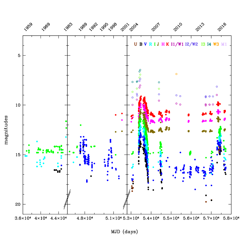
Figure 1: Historical light curve of V1118 Ori. Optical/near-IR and mid-IR magnitudes are represented with filled and open circles, respectively. Magnitudes in different filters are depicted with different colors, as indicated in the top-right label. $UBVRIJHK$ photometry was taken from: Audard et al. 2005, 2010; Garcia Garcia et al. 1995, 2006; Garcia Garcia & Parsamian 2000, 2008; Gasparian & Ohanian 1989; Jurdana-Šepić et al. 2017; Hayakawa et al. 1998; Hillenbrand 1997; Parsamian & Gasparian 1987; Parsamian et al. 1993, 1996, 2002; Papers I, II; Verdenet et al. 1990; Williams et al. 2005. We have also retrived data from the catalogs: AAVSO ($BVRI$), 2MASS ($JHK$), DENIS ($IJK$), WISE (3.4 / 4.6 / 12 $\mu$m, W1-W3), Spitzer/IRAC (3.6 / 4.5 / 5.8 /8.0 $\mu$m, I1-I4), and Spitzer/MIPS (24 $\mu$m, M1).

To have a complete view of the photometric activity of V1118 Ori, we have searched the literature and public archives to construct its multiwavelength historical light curve. This is depicted in Figure 1 (where our new data are also shown) and commented in Section 3.1.1. We collected data since 1959 for the bands $UBVRIJHK$ (references are in the Figure caption), WISE/1-3 (at 3.4 / 4.6 / 12 $\mu$m), Spitzer/IRAC (3.6 / 4.5 / 5.8 /8.0 $\mu$m), and Spitzer/MIPS (24 $\mu$m). Spitzer data are published in Audard et al. (2010), while Wide-field Infrared Survey Explorer (WISE) data are reported here for the first time (Sect. 2.2.3). For completeness, we also account for a few data before 1960s, which indicate a remarkable level of activity ($m_{\rm{pg}}$ $\sim$ 14.0) in 1939, 1956, and 1961 (Paul et al. 1995).

2.2 New photometry

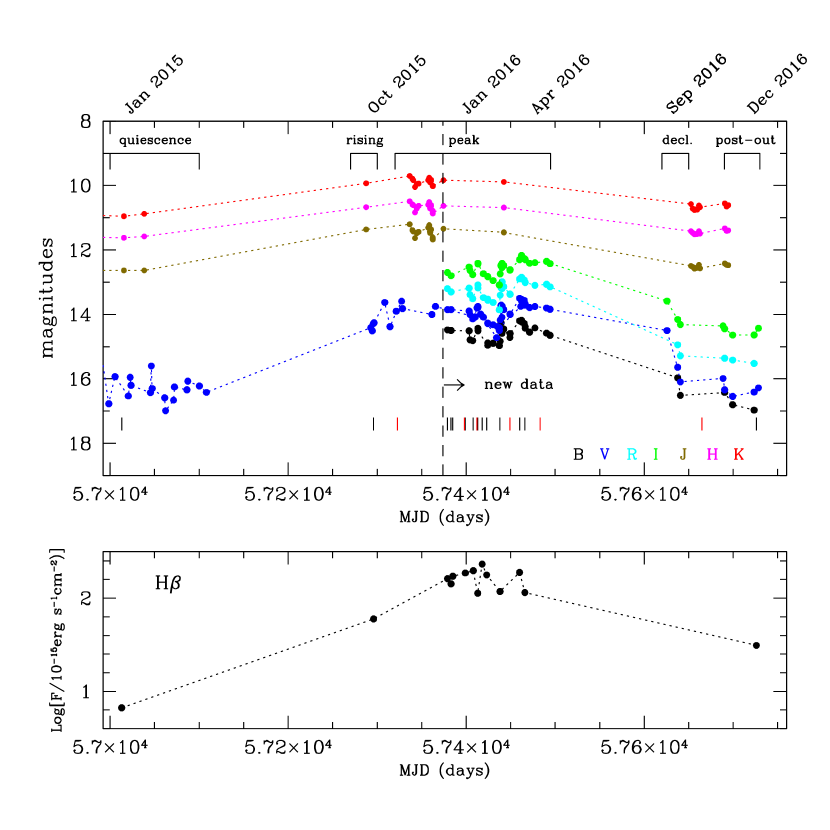
Figure 2: Top panel: optical and near-IR light curve in the period 2015 January-2016 December. Colors indicate the same bands as in Figure 1. Data taken after the date marked with a dashed vertical line are reported in this paper for the first time, while those before that date are taken from the literature. These are shown to have a global view of the 2015-2016 outburst. Different temporal phases are labeled: (1) quiescence: up to 2015 March; (2) rising: 2015 October; /3) peak: 2015 November-2016 April; (4) declining: 2016 September; and (5) post-outburst: since 2016 December. Vertical black and red segments indicate the dates when optical and near-IR spectra were taken. Bottom panel: flux of the H$\beta$ line as a function of time.

The new photometry covers the period 2015 December-2016 December. Together with the photometry reported in Papers I, II it follows the evolution from quiescence to the post-outburst phases. In Figure 2 we show the light curve from 2015 January-2016 December, where we have empirically identified five phases to which we refer in the analysis: (1) quiescence: up to 2015 March; (2) rising: 2015 October; (3) peak: 2015 November-2016 April; (4) declining: 2016 September; and (5) post-outburst: since 2016 December.

2.2.1 Optical photometry

$BVR_{\rm C}I_{\rm C}$ optical photometry of V1118 Ori has been obtained with the Asiago Novae and Symbiotic stars (ANS) Collaboration telescopes 36 and 157, 0.3m $f$/10 instruments located in Cembra and Granarolo (Italy). Technical details and operational procedures of the ANS Collaboration network of telescopes are presented by Munari et al. (2012), while analysis of the photometric performances and multi-epoch measurements of the actual transmission profiles for all the photometric filter sets are discussed by Munari & Moretti (2012). The same local photometric sequence was used at both telescopes in all observing epochs, ensuring a high consistency of the data. The sequence was calibrated from APASS survey data (Henden et al. 2012, Henden & Munari 2014) using the SLOAN-Landolt transformation equations calibrated in Munari (2012) and Munari et al. (2014a,b). Reduction was achieved by using standard procedures for bad-pixel cleaning, bias and dark removal, and flat fielding. All measurements were carried out with aperture photometry, the long focal length of the telescopes and the absence of nearby contaminating stars not requiring to revert to PSF-fitting.

The $BV$$R_{\rm C}$$I_{\rm C}$ photometry of V1118 Ori is given in Table 1 and shown in Figure 2, top panel. The source has remained bright (with daily variations of up to 0.4 mag in $V$) throughout the monitoring period until 2016 April, when observations had to be momentarily alted for Solar conjunction. They restarted in 2016 August, and at that time the visual magnitude dropped by about 1 mag. Since 2016 August, V1118 Ori has continued to rapidly fade to $V\approx$ 16.5 mag, even if it has not reached the magnitude ($V\approx$ 17$-$18 mag) typical of its quiescent state at present.

2.2.2 Near-infrared photometry

$JHK$ aperture photometry was achieved with the 1.1m AZT-24 telescope at Campo Imperatore (L’Aquila, Italy) with the SWIRCAM camera (D’Alessio et al. 2000). Data reduction was performed by using standard procedures for bad-pixel cleaning, flat fielding, and sky subtraction. Calibration was achieved on the basis of $2MASS$ photometry of several bright stars in the field. We present in Table 2 and Figure 2 (top panel) the data obtained between 2015 December and 2016 November, which follow those provided in Papers I and II. The peak of the infrared activity occurred between 2015 December and 2016 February. No data are available between 2016 March and September; after this period, the source has faded and reached the quiescence value in all the near-IR bands (see Paper I).

2.2.3 WISE photometry

V1118 Ori was also observed in its quiescent phase by WISE, (Wright et al. 2010) during both the cryogenic (2009 December 2009 - 2010 August) and the 3-band (2010 August - September) surveys (see Table 3). Average values of the WISE magnitudes are [3.4] = 9.9, [4.6] = 9.0, [12] = 6.9, and [22] $>$ 3.4 mag. More recent observations have been collected in the first two bands during the ongoing Neowise-R survey. Measurements taken on 2015 September 16 are [3.4] = 8.9 and [4.6] = 8.1, with a brightness increase of $\approx$ 1 mag in both bands with respect to the quiescence values.

2.3 Spectroscopy

V1118 Ori has been spectroscopically observed in low- and high-resolution configurations at optical and near-IR wavelengths. A journal of the spectroscopic observations is given in Table 4.

2.3.1 Optical spectroscopy

Four optical low-resolution spectra have been collected on 2016 January 12, 26, and 31 and 2016 December 4 with the 8.4 m Large Binocular Telescope (LBT) using the Multi-Object Double Spectrograph (MODS - Pogge et al. 2010). All observations have been taken with the dual grating mode (Blue + Red channels) and integrated 1500 s in the spectral range 3200$-$9500 Å  by using a 0$\farcs$8 slit ($\Re\sim$ 1500). Data reduction was performed at the Italian LBT Spectroscopic Reduction Center by means of scripts optimized for LBT data. Steps of the data reduction of each two-dimensional spectral image are correction for dark and bias, bad-pixel mapping, flat-fielding, sky background subtraction, and extraction of one-dimensional spectrum by integrating the stellar trace along the spatial direction. Wavelength calibration was obtained from the spectra of arc lamps, while flux calibration was achieved using the ANS Collaboration telescopes photometry, taken within one day from the spectroscopic observations.

Seven additional spectra (3300$-$8050 Å) at $\Re$ $\sim$ 2400 were obtained with the 1.22m telescope + B&C spectrograph operated in Asiago by the University of Padova. The slit has been kept fixed at a width of 2$\arcsec$ and was always aligned with the parallactic angle for optimal absolute flux calibration.

Finally, six high-resolution spectra in the range 3600$-$7300 Å  were taken with the REOSC Echelle spectrograph mounted on the 1.82m telescope operated in Asiago by the National Institute of Astrophysics (INAF). The spectrograph covers the whole wavelength interval in 32 orders without interorder gaps. The slit width was set to provide a resolving power of 20 000, and - as for the 1.22m - the slit was always aligned with the parallactic angle for optimal absolute flux calibration.

The spectra from the Atwo siago telescopes were reduced within IRAF following all the steps cited above for the reduction of the MODS spectra. Flux calibration was achieved by means of standards observed at similar airmass before and after V1118 Ori. While this ensures an excellent correction of the instrumental response, the zero-point of the flux scale was sometimes affected by the unstable sky transparency. Check (and correction whenever necessary, always $\leq$30%) of the zero-point has been performed by integrating on the spectrum the flux through the $B$,$V$ and $R$-band profiles and comparing to values from the photometric campaign.

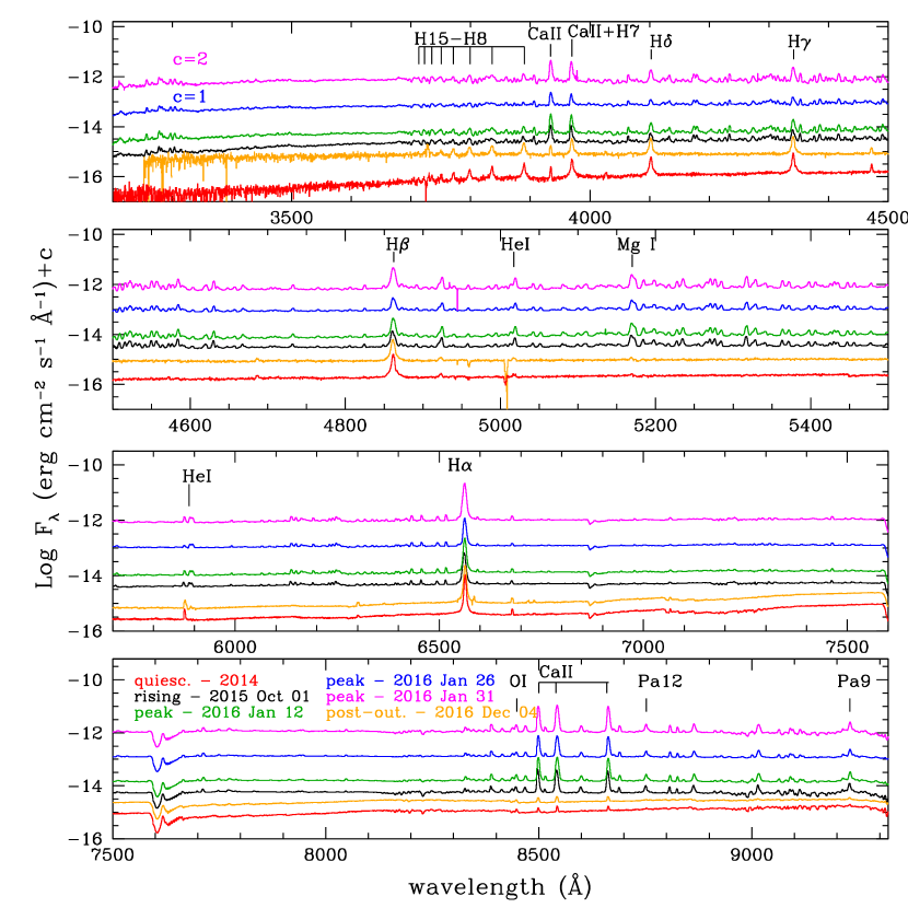
Figure 3: Optical (LBT/MODS) spectra of V1118 Ori taken in 2016 January (peak: green, blue, and pink) and 2016 December (post-outburst: orange), shown in comparison with the spectra taken in quiescence (red, Paper I) and during the rising phase (black, Paper II). For a better visualization a constant (indicated in the top panel) was added to the spectra taken on January 26 and 31. Main emission lines are labeled.

In Figure 3 the four MODS spectra are depicted in comparison with the quiescence spectrum (Paper I) and that obtained during the rising phase (Paper II). The same forest of lines as observed in the 2015 October spectrum is present in the burst spectra, but further increased in brightness. The large majority are recombination lines or lines of neutral and ionized metals (H I, He I, Ca II, Fe I, and Fe II), most of them blended with each other. We give in Table 5 the line fluxes of bright and unblended lines that are used in the spectral analysis. Their flux is computed by integrating the signal below the spectral profile. The FWHM is compatible with the instrumental one because the lines are not resolved in velocity at the adopted resolution. The associated uncertainty is estimated by evaluating the rms in a wavelength range close to the line, and then multiplying it by the FWHM.

The low-resolution Asiago spectra are shown in Figure 4. Together with H I  and Ca II  lines, other features of metallic lines are prominent in the spectrum, but they result from blends of two or more lines, so their flux is not useful for the line analysis.

Most of the permitted lines that appear blended in the optical low-resolution spectrum are clearly identified at the spectral resolution achieved in the echelle spectra. A list and comments on these lines are provided in Appendix A and in Section 3.2.4, respectively. Profiles of the most interesting lines (in particular the Balmer lines) are presented in Section 3.3.

Fluxes of unblended bright lines observed with the Asiago telescopes are listed in Table 6. The sensitivity limit is about a factor of ten lower than the limit of MODS, therefore reliable fluxes can be given only for some permitted lines (not reported in Table 6), along with the Balmer and Ca II  H lines. Whenever both a low- and a high-resolution spectrum is available at a certain date, the fluxes agree each other within 20%, with the exception of the flux of H$\alpha$, which shows prominent wings that are better resolved at higher dispersion. In Table 6 we therefore give the average of the two determinations, except for H$\alpha$, for which we report the flux measured in the high-resolution spectrum.

Finally, we note that many lines present a remarkable level of variability on timescales of days (see Tables 5 and 6). For example, H$\alpha$ and H$\beta$ fluxes increase by about a factor of two from January 26 to 31. As we show as an example in the bottom panel of Figure 2, the variation of F(H$\beta$) roughly follows that of the continuum, although with a certain delay. In particular, the continuum fades faster than lines. This is evident for the last spectroscopic point (MJD 57726), when the continuum level was close to that of quiescence (top panel), while F(H$\beta$) was still about a factor of 5 brighter. This circumstance appears to be a common feature of EXor variability (Paper I).

2.3.2 Near-IR spectroscopy

Three near-infrared, low-resolution spectra have been obtained with the LUCI2 instrument at LBT on 2016 January 25, March 2, and October 4. The observations were carried out with the G200 low-resolution grating coupled with the 1$\farcs$0 slit on the first two dates and with the 0$\farcs$75 slit on October 4. The standard ABB’A’ technique was adopted to perform the observations using the $zJ$ and $HK$ grisms, for a total integration time of 12 and 8 minutes, respectively. The final spectrum covers the wavelength range 1.0$-$2.4 $\mu$m at $\Re\sim$1000. Data reduction was performed at the Italian LBT Spectroscopic Reduction Center. The raw spectral images were flat-fielded, sky-subtracted, and corrected for optical distortions in both the spatial and spectral directions. Telluric absorptions were removed using the normalized spectrum of a telluric standard star, after fitting its intrinsic spectral features. Wavelength calibration was obtained from arc lamps, while flux calibration was achieved through the observations of spectrophotometric standards, carried out in the same night as the target. No intercalibration was performed between the $zJ$ and $HK$ parts of the spectrum, since they were optimally aligned. We evaluated possible flux losses by comparing the continuum level at the $JHK$ effective wavelengths (1.25, 1.60, and 2.20 $\mu$m) with the magnitudes of the closest photometric points, obtained within a week from the spectroscopic observations. While for the first two spectra (January 25 and March 2), the agreement is within 20%, significant flux losses, mainly due to the bad weather conditions during the observation, are registered in the spectrum of October 4. Therefore we used the photometric data of October 1 to calibrate this spectrum, which in any case is much fainter than the first two. No intercalibration was applied between near-IR and optical spectra as they all were acquired on different dates.

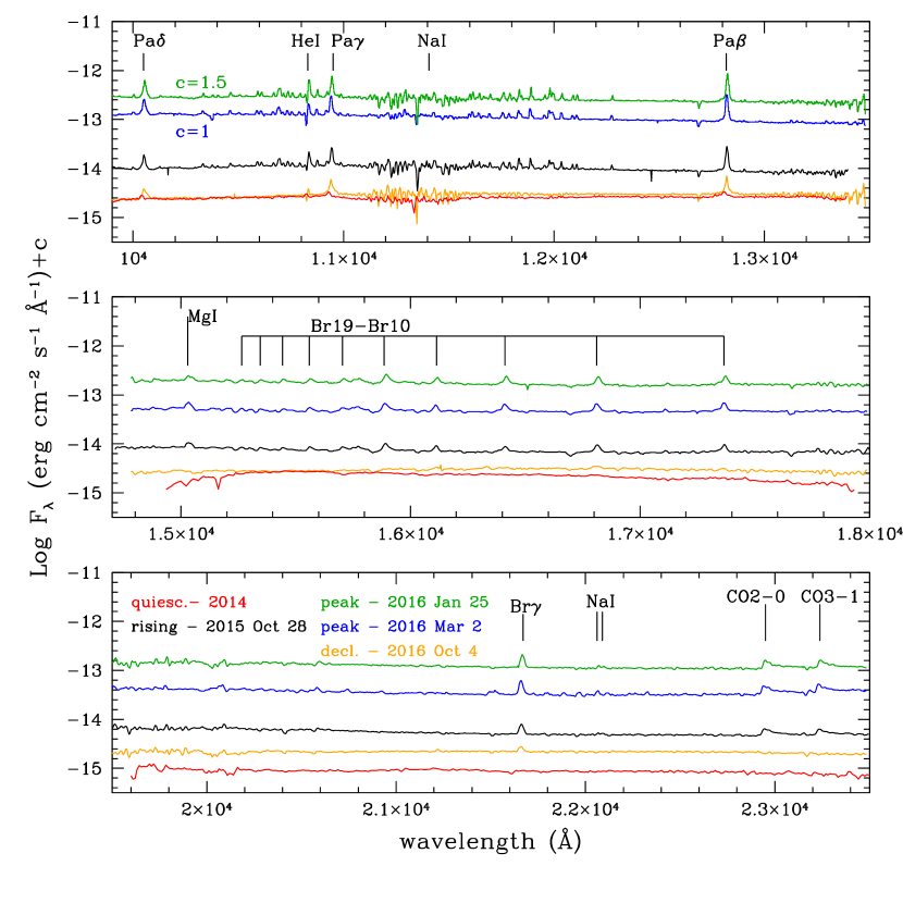
Figure 5: Near-IR LUCI2 spectra taken on 2016 January and March (peak: green, blue), and 2016 October (declining: orange) in comparison with spectra taken in quiescence (red, Paper I) and during the rising phase (black, Paper II). For a better visualization a constant (indicated in the top panel) was added to the spectra taken on January 25 and March 2. Main emission lines are labeled.

The three LUCI2 spectra are shown in Figure 5, in comparison with the spectra taken in quiescence (Paper I) and during the rising phase (Paper II). Fluxes of the main unblended lines are listed in Table 7. In the peak phase the most prominent lines are H I  recombination lines of the Paschen and Brackett series, He I  1.08 $\mu$m, Mg I, and Na I  lines. CO 2-0 and 3-1 ro-vibrational bands are also observed in emission. Other metallic lines are likely present, but they are too faint or strongly blended to be clearly identified. In the last spectrum, taken during the declining phase, we detect the brightest H I  lines, He I  1.08 $\mu$m, and H₂ 2.12 $\mu$m. Notably, while H I  line fluxes are similar to those during the rising phase (Paper II), the continuum level is closer to the quiescence level. This confirms what we have already noted about the optical lines in Sect.2.3.1.

Near-IR, high-resolution spectra were obtained on 2016 January 10 and 2016 April 05 with GIANO at the Telescopio Nazionale Galileo (La Palma. Spain) during two Director Discretionary Time (DDT) runs. GIANO provides in a single-exposure cross dispersed echelle spectroscopy at a resolution of 50 000 ($\delta$v $\sim$ 6 km s^-1 at $\lambda$ =  1 $\mu$m) over the 0.95-2.45 $\mu$m spectral range. Since at longer wavelengths the echelle orders become larger than the 2k$\times$2k detector, the spectral coverage in the $K$ band is 75%, with gaps, for example, at the Br$\gamma$ and CO 1-0 wavelengths. GIANO is fiber-fed with two fibers of 1$\arcsec$ angular diameter at a fixed angular distance of 3$\arcsec$ on sky. The science target is acquired by nodding on fiber, namely alternatively acquiring target and sky on fibers A and B, and vice versa. This allows an optimal subtraction of the detector pattern and sky background. Data reduction was achieved by means of specific scripts optimized for GIANO . In particular, observations of a uranium-neon lamp were carried out to perform wavelength calibration, while flat-fielding and mapping of the order geometry were achieved through exposures with a tungsten calibration lamp. The reduced spectrum is rich in metallic lines that were barely detected in the low-resolution spectrum, which we list in Appendix B and comment in Section  3.2.4. Profiles of the most interesting lines (H I  lines and He I  1.08  $\mu$m) are presented in Section 3.3.

3 Analysis and Discussion

3.1 Photometric analysis

3.1.1 Light curve

The 2015-2016 outburst is the sixth documented during the recent history (about 40 years) of V1118 Ori; previous events (1983, 1989, 1992, 1997, and 2005) are recognizable in the light curve in Figure 1. This global view of the V1118 Ori photometric behavior shows two facts: (1) the present outburst is roughly at the same intensity level ($V_{peak}\sim$ 13.5 mag) and duration ($\sim$ 1 year) as the bursts that occurred between 1989 and 1997, whereas the outburst occurred in 2005 has been the brightest ($V_{peak}\sim$ 12 mag) and maybe the longest ($\gtrsim$ 2 years); (2) in the course of time the monitoring improved progressively in both sampling cadence and spectral coverage. In particular, systematic observations have shown that V1118 Ori has remained quiescent for about a decade (from 2006 to 2015). Indeed, four out of the five previously known events have occurred with a roughly regular cadence of 6-8 years, with the only exception the outburst occurred in 1992 (Garcia Garcia et al. 1995), which was much fainter than all the others ($V\leq$ 14.7 mag), however. The evidence that the 2015 outburst is not in phase with the previous outbursts, does not support periodic phenomena as the cause of the outburst triggering. A quiescence period of about 15 years (from 1966 to 1981) has also been shown by a recent analysis of historical plates (Jurdana-Šepić et al. 2017).

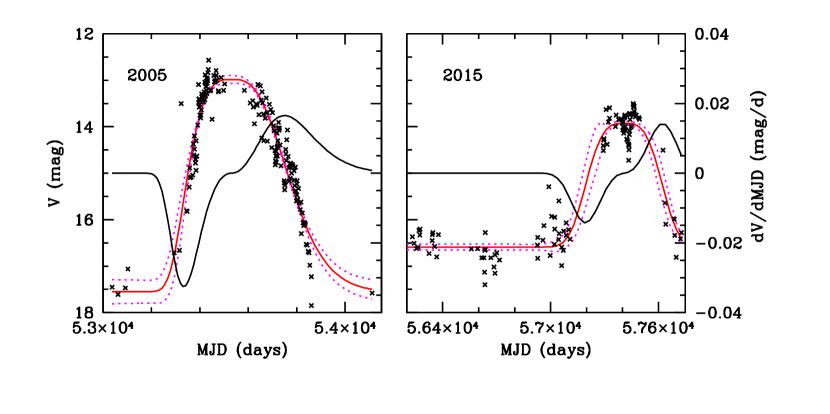
Figure 6: Left panel: $V$ light curve of the 2005 outburst. The red solid curve is the best distorted Gaussian through the data points, whose uncertainty is represented by the pink dotted lines. The black solid line is the derivative of the distorted Gaussian, which represents the velocity in magnitude variation. Right panel: the same as in the left panel for the 2015 outburst. A large portion of the light curve before the outburst is plotted to show the quiescence level.

We have compared the present outburst with the outburst of 2005 to understand whether they have followed a similar evolution in time. In Figure 6 the $V$ light curves of the 2005 and 2015 outbursts are shown in the left and right panel, respectively. While the 2005 outburst has occurred as a sudden event starting from a very faint level ($V\,\gtrsim$ 17.5 mag), the outburst of 2015 followed a long period that was characterized by a higher average brightness ($<V>$ $\sim$ 16.5 mag) with daily scale fluctuation of several tens of magnitude, presumably unrelated with the accretion burst. Quantitatively, the two light curves (covering about 1200 days each) have been fitted with a single distorted Gaussian This is depicted as a red solid curve, while the fit uncertainty is represented with pink dotted lines. The derivative to the fitted Gaussian (black line) allows us to account for the speed typical of the different outburst phases. In 2005, the rising speed has increased monotonically to values ($\sim$ 0.035 mag/day) about twice the decreasing speed ($\sim$ 0.015 mag/day). Notably, the 2015 outburst is characterized by a similar rising and declining speed ($\sim$ 0.015 mag/day). This might indicate that while triggering has occurred under different modalities, the relaxing phenomenon has followed as similar evolution.

In conclusion, as also confirmed by spectroscopic data, see Sect.3.2.2, the 2015 outburst appears different from the outburst in 2005, as far as intensity, duration, recurrence time, and rising speed are concerned. Whether the observed behavior is specific of V1118 Ori, or is more in general a common feature of the EXor variability, remains an open question. For the moment, the possible comparison is with the candidate EXor V2492 Cyg, which shows a slower rising than declining speed, although the variability of this source is not fully due to disk-accretion phenomena (Hillenbrand et al. 2013).

3.1.2 Color analysis

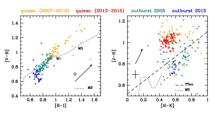
Figure 7: Left panel: optical two-color plot [$V-R$] vs. [$R-I$]. Orange/red crosses: quiescence data ($V\geq$ 15) in the periods 2007-2010/2013-2015; teal-blue/blue crosses: 2005/2015 outbursts data ($V<$ 15). References: present paper; Audard et al. 2010. Dotted line: unreddened main-sequence. Colors of M1 and M3 stars are indicated. Arrow: extinction vector corresponding to A_V =  1 mag (reddening law of Cardelli et al. 1989). The average error is indicated with a black cross. Right panel: the same as in the left panel for the near-IR two color plot [$J-H$] vs. [$H-K$]. Quiescence and outburst are defined as $H\geq$ 11 and $H<$ 11, respectively. References: present paper; Papers I, II; Audard et al. 2010. Dashed line: locus of the T Tauri stars (Meyer et al. 1997).

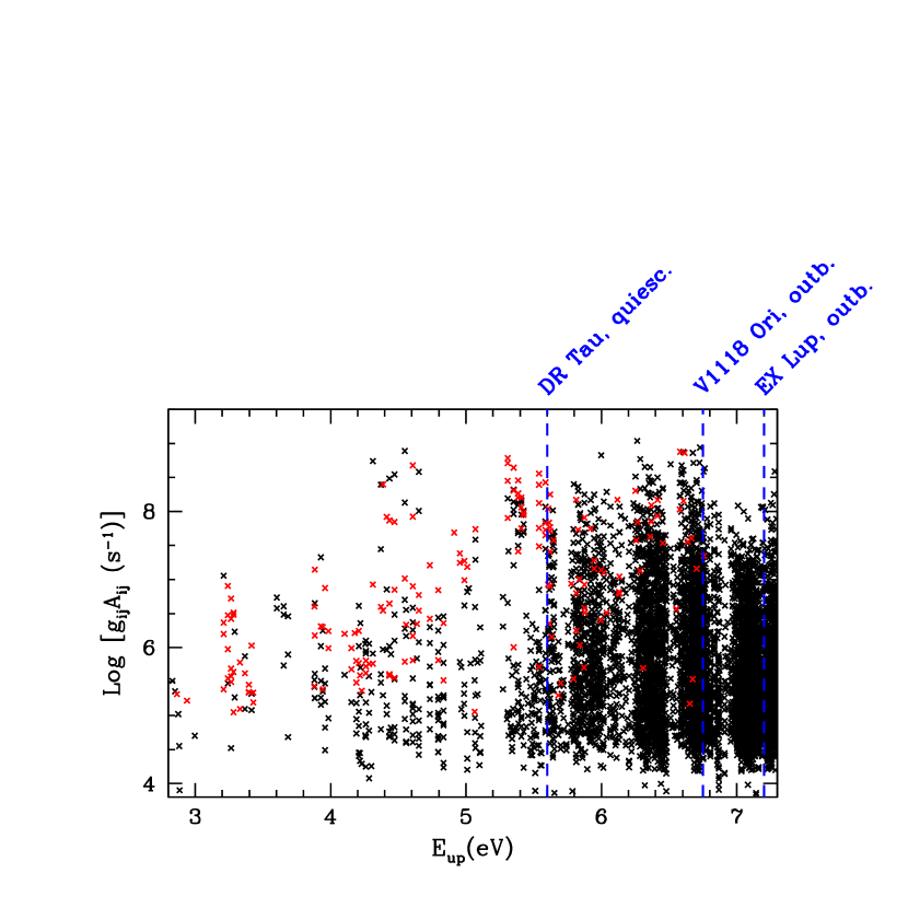
Figure 11: Einstein coefficients $\times$ statistical weight (g_ijA_ji) of Fe I lines between 4 000 and 20 000 Å  as a function of the energy of the upper level (black dots). Lines observed in V1118 Ori are represented in red. Blue lines indicate the energy of the line with the highest value of E_up observed in DR Tau (Beristain et al. 1998), V1118 Ori, and EX Lup (Sicilia-Aguilar et al. 2012).

To investigate the origin of the photometric fluctuation, we plot in Figure 7, left panel, the optical [$V-R$] vs. [$R-I$] colors of V1118 Ori measured during quiescence and recent outbursts (2005 and 2015). These are obtained by combining the data of the present paper with those by Audard et al. (2010). Quiescence and outburst phases are identified by $V$ lower or greater, respectively, than 15 mag. The data points of the 2015 outburst follow a similar distribution as those of 2005. As has been shown by Audard et al. (their Figure 11), colors become bluer with increasing brightness, moving almost parallel to the reddening vector in the direction of a decreasing extinction. However, although a variable extinction certainly plays a role (see also Sect. 3.2.1), it cannot be the primary cause of the brightness enhancement typical of outbursts. Indeed, as shown in the Figure, the colors of an unreddened main-sequence star of the V1118 Ori spectral type (M1-M3) are typically redder than the outburst colors. Instead, and in agreement with previous studies on EXors (Audard et al. 2010; Lorenzetti et al. 2012), we interpret the blueing of the optical colors as mainly due to a hotter temperature component appearing during the outburst. Note that in this view the extinction may even increase during outburst, but not enough to compensate for the blueing of the color indices.

The near-IR [$J-H$] vs. [$H-K$] color diagram (Figure 7, right panel) is in agreement with the above interpretation. Indeed, although colors of the different phases (quiescence: $H\geq 11$, outburst: $H<11$) spread over a large portion of the plot, they roughly segregate into two different portions of the plot, whose connecting direction does not follow that of the reddening vector.

3.2 Line analysis

3.2.1 Extinction estimate

As a first step of the line analysis, we have estimated the extinction toward V1118 Ori. A common and powerful tool to achieve this is to use pairs of optically thin and bright transitions coming from the same upper level, since in this case the difference between observed and theoretical flux ratio depends only on the extinction value. We have considered pairs of H I  lines whose profiles do not seem affected by evident opacity effects, such as self-absorption or flatted peaks (see Sect.3.3). These are Pa$\beta$/H$\gamma$, Pa$\gamma$/H$\delta$, Pa9/H9, Pa12/H12, and Br$\gamma$/Pa$\delta$. Considering all the available spectra, we estimate A_V in the range 1.5$-$2.9 mag, without any significant trend between quiescence and outburst phases. Indeed, extinction fluctuations up to 1 mag are also recognizable in the color-color diagrams of Figure  7.

As an alternative method, we estimate A_V by modeling and fitting the uv/optical MODS continuum (Section 3.2.2). In good agreement with the range found from line ratios, the best fit provides A_V = 2.9 mag in quiescence, rising, and at the outburst peak, and A_V = 1.9  mag in the post-outburst phase.

For comparison, our A_V estimate is also compatible with that between 1.4 and 1.7 mag obtained by Audard et al. (2010) on the basis of X-ray observations during the outburst of 2005.

Summarizing, since our analysis is largely based on the uv/optical lines and continua, an A_V intrinsic variability of about 1 mag might significantly reflect on the estimate of physical parameters and mass accretion rate. Therefore, in the following we will consider conservatively the two extreme values of A_V, namely 1.5 and 2.9 mag. This will give us an idea of how much the A_V variability influences the results.

3.2.2 Mass accretion rate

To determine the mass accretion rate ($\dot{M}_{acc}$) we applied two different methods (indeed not strictly independent) involving both continuum and emission lines.

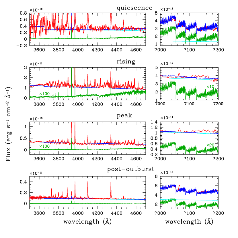
Figure 8: Top panel: dereddened spectrum (A_V = 2.9 mag) of V1118 Ori between 3500$-$4700 Å  and 7000$-$7200 Å, during quiescence (red). The spectrum of an M3 star template is shown in green. The continuum excess emission of the slab model is plotted in cyan, while the best fit with the emission predicted from the slab model added to the template is given by the blue line. Other panels: the same as in the top panel for the rising, peak, and post-outburst phases. In this latter, the spectrum was dereddened for A_V = 1.9 mag. For a better visualization, the template spectrum has been multiplied by a constant where indicated.

In the first method, described in Manara et al. (2013), we fitted the observed MODS spectrum in various continuum regions from $\sim$3200 Å  to $\sim$7500 Å  using the sum of a photospheric template and a slab model to reproduce the continuum excess emission due to accretion. We adopted the reddening law by Cardelli et al. (1989) with $R_{V}$ = 3.1. We first fitted the quiescence spectrum taking as free both the stellar parameters and the extinction value. The best fit (Fig. 8, top panel), is obtained with a photospheric template of spectral type (SpT) M3 and for $A_{V}$ = 2.9 mag (as anticipated in the previous Section). These lead to $R_{\mathrm{*}}$ = 1.67 R_⊙  and $L_{\star}$ = 0.32 $L_{\odot}$, when a distance of 414 pc is adopted. By assuming the evolutionary models of Baraffe et al. (2015), the fitted parameters correspond to $M_{\mathrm{*}}$ = 0.29 M_⊙ . According to our working plan, we also fitted the quiescence spectrum adopting $A_{V}$ = 1.5 mag (not shown in the Figure). The fit gives SpT =  M3, $R_{\mathrm{*}}$ = 1.07 R_⊙ , $L_{\star}$ = 0.18 $L_{\odot}$, and $M_{\mathrm{*}}$ = 0.29 M_⊙ .

Fits of the subsequent phases (rising, peak, and post-outburst, Fig. 8, second, third, and fourth panel) were made by assuming the stellar parameters fitted in quiescence, and keeping $A_{V}$ and SpT fixed. We varied the contribution of the slab to the emission until a best fit was found. This is the same procedure as adopted to fit DR Tau by Banzatti et al. (2014). The fit of the rising and peak spectra, in particular, is very uncertain because the continuum emission is dominated by the accretion shock. The $\dot{M}_{acc}$  derived with this ’Continuum’ (C) method are listed in Table 8, first and second column.

As a second method, we applied the empirical relationships derived by Alcalá et al. (2016) between line and accretion luminosity ($L_{\mathrm{acc}}$)  for a sample of young active T Tauri stars in Lupus. We assumed the same parameter values as for the continuum fitting, which were also taken to recompute the mass accretion rate in quiescence and rising phases (given in Papers I and II). This allows us to meaningfully compare the results. We applied the Alcalá et al. relationships to the brightest H I  lines (those detected with S/N $\gtrsim$ 10), which are the Balmer lines in the MODS and Asiago spectra, and the Paschen and Br$\gamma$ lines in the LUCI2 spectra. Finally, we converted $L_{\mathrm{acc}}$  into $\dot{M}_{acc}$ by applying the relationship reported by Gullbring et al. (1998). The results are summarized in Table 8, third and fourth column (’Line’ (L) method).

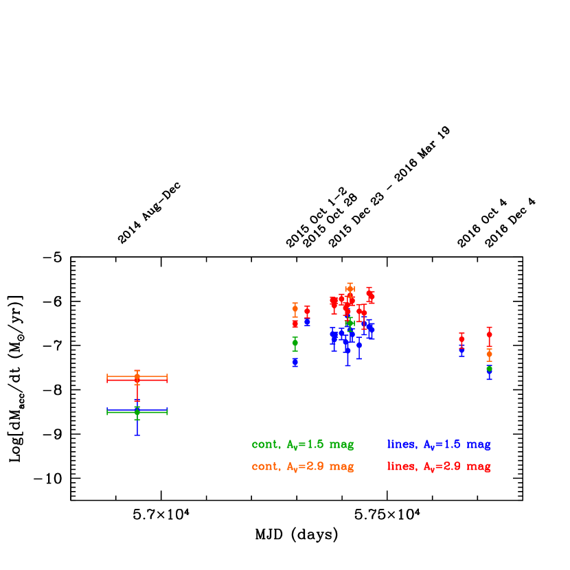
Figure 9: Mass accretion rate as a function of time. With different colors we depict $\dot{M}_{acc}$  values derived under different assumptions for the fitting method or the adopted extinction. Determinations of $\dot{M}_{acc}$  that refer to 2014 August-December and 2015 October have been obtained from the spectra published in Papers I and II, respectively.

The $\dot{M}_{acc}$  values are also shown in Figure 9, where different colors are used to represent the adopted fitting method and extinction value. $\dot{M}_{acc}$  increased by about two orders of magnitude from quiescence to the outburst peak, going from 0.3 $-$ 2.0 10^-8 M_⊙ yr^-1 to 0.2 $-$ 1.9 10^-6 M_⊙ yr^-1 . The upper end value is close to the estimate by Audard et al. (2010) at the peak of the 2005 outburst, obtained by means of Spectral Energy Distribution (SED) fitting. Given the higher brightness attained by the 2005 outburst, its mass accretion rate should presumably be higher than for the 2015 event.

For a fixed A_V, the $\dot{M}_{acc}$  derived with the two methods is consistent within the uncertainties, with the only exception that of the rising phase; conversely, differences of up to a factor of four are found between $\dot{M}_{acc}$  derived under a different A_V assumption. Since these differences are a due to the intrinsic, short-timescale variability of V1118 Ori, and not to a poor determination of A_V, the extreme $\dot{M}_{acc}$  values have to be taken as the lower and upper end values that characterize the considered temporal phase.

Finally, it is also interesting to note that $\dot{M}_{acc}$ (post-outburst) $\approx$ $\dot{M}_{acc}$ (rising), even if the continuum level is very close to the quiescence value. This result is a direct consequence of the slower decrease of the line fluxes, as we have shown in Figure 2 for the case of the H$\beta$ flux.

3.2.3 Hydrogen physical conditions

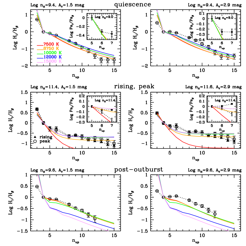
Figure 10: Balmer decrements (H_i/H$\beta$ flux ratios vs. upper level of the transition) in quiescence (top panels), rising/peak (central panels), and post-outburst phases (bottom panels). In the left and right panels the observed ratios are corrected for A_V =  1.5 mag and 2.9 mag, respectively. The fluxes have been normalized to the H$\beta$ flux. The observations have been fitted with the local line excitation models of Kwan & Fischer (2011). Models with different temperatures are depicted with different colors, and the adopted density is labeled. In the insets, the Paschen decrements (normalized to the Pa$\beta$) are shown and compared with the relative predictions of Edwards et al. (2013).

To derive the physical conditions of the gas that emits the H I  lines, we have compared the observed Balmer decrements (plots of flux ratios vs. upper level of the transition) with the predictions of the local line excitation computation by Kwan & Fischer (2011), who provide a grid of models in the range of hydrogen density log [$n_{\rm{H}}$ (cm^-3)] = 8-12 and temperature between 3750 K and 15 000 K. We have also examined the Paschen decrements for the few lines we observe, and compared them with the models by Edwards et al. (2013). We show the results in Figure 10, where Balmer (from MODS spectra) and Paschen (from LUCI2 spectra) decrements are represented in the large panels and the insets, respectively. Since the H$\alpha$ line can be severely contaminated by opacity effects and chromospheric emission, we preferred to use the H$\beta$ as a reference line for the Balmer decrements (e.g. Antoniucci et al. 2017). Furthermore, as the decrement shape may vary depending on the adopted reference line, we have verified that using lines with a higher n_up as reference does not provide significantly different results from those reported here. The Paschen decrements have been normalized to the Pa$\beta$ line.

Balmer decrements during the quiescence phase are shown in the top panels, after they have been corrected for A_V = 1.5 mag (left) and A_V = 2.9 mag (right). Regardless of the adopted extinction value, the decrement shape resembles the straight type 2 shape cataloged by Antoniucci et al. (2017). To this class of decrements typically belong T Tauri sources with $\dot{M}_{acc}$  in the range -10.8 $<$ log [$\dot{M}_{acc}$(M_⊙ yr^-1)]$<$ -8.8, in good agreement with our estimates of Section 3.2.2. For the two A_V values, we find that models with log [$n_{\rm{H}}$ (cm^-3)] = 9.4 are those that best fit the observed decrements, even if the overall shape is not well reproduced. No significant constraint can be placed on the hydrogen temperature from the Balmer decrements alone. While lower temperatures seem favored when A_V = 1.5 mag is adopted, the opposite occurs for A_V = 2.9 mag. The Paschen decrements, although not well fitted by models, suggest $T\lesssim$ 10 000 K.

In the central panels we show the Balmer decrements of the rising (triangles) and peak (circles) phases. The most important difference with respect to quiescence is the enhancement of the ratios of lines with n_up $\gtrsim$ 10 of at least an order of magnitude. When compared with the decrement classification of Antoniucci et al., rising and peak decrements resemble the $L-shape$ type 4 decrements, observed mostly in objects with log [$\dot{M}_{acc}$(M_⊙ yr^-1)] $>$ -8.8. Again according to the Kwan & Fischer models, the hydrogen density has increased by about two orders of magnitude with respect to quiescence, while temperatures between 8750 and 15 000 K are suggested by both the Balmer and Paschen decrements.

In the bottom panels we show the Balmer decrements of the post-outburst phase. Their shape is of type 3, or (bumpy), according to the definition of Antoniucci et al., which is intermediate between types 2 and 4 (-9.8 $<$ log [$\dot{M}_{acc}$(M_⊙ yr^-1)]$<$ -8.8). A good agreement between models and data is found only for log [$n_{\rm{H}}$ (cm^-3)] = 9.6, T$\lesssim$ 10 000 K and A_V = 1.5 mag.

We can conclude that the physical conditions of the gas profoundly changed from quiescence to outburst, and this is especially true for the gas density. We can argue that this has led also to a similar enhancement in the accretion column density and consequently in the mass accretion rate.

3.2.4 Other lines

The high-resolution Asiago (echelle) and TNG (GIANO) spectra display a number of unblended emission lines of neutral atoms typical of M-type stars (e.g. Na, Ca, Fe, Ti, and Si, see Appendices A and B). Because of their low-ionization potential (between 5 and 8 eV), these lines likely originate in neutral regions close to the disk surface, far enough from the central star and accretion columns to prevent their ionization, but still reached by stellar UV photons able to populate energy levels close to the continuum, however. In Table 9 we list for each metallic species the energy of the most highly excited line, max(E_up), and the number of detected lines, N_lines. The reported statistics is done considering only the optical lines (in the 3300$-$7300 Å  range covered at high resolution), since this allows a meaningful comparison with the optical spectrum of EX Lup, taken during its 2008 outburst by Sicilia-Aguilar et al. (2012). As we show in the last two columns of Table 9, the EX Lup spectrum is definitely richer of high-excitation lines. This suggests that in this source the accretion shock produces more energetic photons or that the radiation shielding is less efficient in its environment. It is interesting, however, that in contrast to this general trend, much more highly excited lines of Ti I and V I are detected in V1118 Ori. Very likely, both these species are almost completely ionized in EX Lup, given their low-ionization potential (6.8 eV for Ti I and 6.7 eV for V I). Finally, we report the detection of Li I  6707 Å  in emission (S/N $\sim$ 4), a feature that is also present in the outburst of 2005 (Herbig 2008). This line is usually absent or seen in absorption in the spectra of classical T Tauri stars.

It is interesting to perform a more in-depth study of the Fe I lines that dominate the emission spectrum during the outburst. For this study we have considered all the Fe I lines predicted by theory with $\lambda$ between 4000 and 20 000 Å  and inside the atmospheric windows, but discarding those with $A$ Einstein coefficients $\leq$ 10³ s^-1 or energy of the upper level E_up $\geq$ 7.15 eV. The atomic data ($A-$coefficients, statistical weights and E_up values) are taken from ’The atomic line list’, v.2.05b21, http://www.pa.uky.edu/ peter/newpage/. In Figure 11 we plot as black crosses the theoretical product g_ijA_ij (statistical weight $\times$ Einstein coefficient) of the Fe I lines as a function of E_up. This product is proportional to the line intensity, and therefore it gives an idea of the brightest lines depending on the level of the gas excitation. With red crosses we indicate the lines observed in V1118 Ori. Although with exceptions, we observe the lines having g_ijA_ij $\gtrsim$ 5 10⁵ s^-1 for E_up $\lesssim$ 6.5 eV and g_ijA_ij $\gtrsim$ 10⁷ s^-1 for E_up $\gtrsim$ 6.5 eV. We do not observe lines having E_up $>$ 6.7 eV, a value in between the maximum E_up of lines observed in DR Tau (in quiescence, Beristain et al 1998) and in EX Lup (during outburst, Sicilia-Aguilar et al. 2012).

Indications of the temperature and density of the line-emitting regions can be derived from the ratios of bright lines. The three Ca II  emission lines at $\lambda\lambda$ 8498, 8542, and 8662 Å  remained roughly constant throughout the outburst duration with ratios close to unity, which are suggestive of optically thick environments. According to the analysis of a sample of Herbig stars, Hamann & Persson (1992) have estimated that Ca II  optically thick lines are produced for an electron density of 10¹¹ cm^-3 and a hydrogen column density $\geq$ 10²¹ cm^-2, if the temperature is between 4000 and 10 000 K. Indeed, we can set as upper limit the maximum hydrogen temperature of $\sim$ 15 000 K derived from the analysis of the Balmer lines (Sect.3.2.3), and as a lower limit the few thousand Kelvin (typically $\lesssim$ 4000 K) that are typically traced by the emission of the CO ro-vibrational bands (see below).

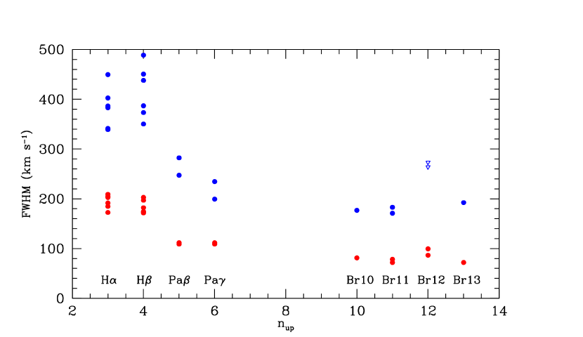
Figure 14: FHWM of the brigthest H I  lines plotted against n_up. Red and blue dots represent the narrow and broad component, respectively. Triangles indicate upper limits on the FWHM of the Br12 line (see text). Multiple points of the same line refer to different dates of observation.

Other remarkable lines are the O I  triplet at 1.29 $\mu$m, pumped by the Ly$\beta$ (McGregor et al. 1988), and whose de-excitation originates the 8446 Å , and the Na I  2.206, 2.207 $\mu$m doublet. Lorenzetti et al. (2009, their Figure 14) noted that in EXor spectra the Na I  doublet is detected both in emission and in absorption following the same behavior of the CO bands. Usually, strong CO emission is seen during outburst phases, while a progressive fading, absence, or absorption is detected as the outburst proceeds toward the quiescence (e.g. Aspin 2008 and references therein; Biscaya et al. 1997; Hillenbrand et al. 2013). This is also seen in V1118 Ori: neither quiescent nor declining spectra show either CO bands or the Na I doublet, while in outburst both species are seen in emission (Figure 5). The common origin of CO and Na I  emission is likely due to the very low-ionization potential of neutral sodium (5.1 eV), which can survive only close to low-mass late-type stars (like EXor, T Tauri, e.g. Antoniucci et al. 2008), and more generally, in regions deep enough inside the circumstellar disks where CO ro-vibrational bands are collisionally excited and shielding against photons that are able to produce Na⁺ is efficient (McGregor et al. 1988). These conditions require densities $>$10⁷ cm^-3 and only moderately warm temperatures, because CO is completely dissociated at $\sim$4000 K.

The [O I] 6300 Å  line is the only forbidden optical line present in the V1118 Ori spectrum (at an S/N $\sim$ 6$-$8). In the Asiago high-resolution spectra, the line presents a structured profile that can be deconvolved into two components, one close to the peak of the diffuse [O I] 6300 Å  in the Orion nebula (v${}_{helio}\sim$ +30 km s^-1, García-Díaz & Henney 2007), and a blue-shifted component centered at v${}_{helio}\sim$ $-$15 km s^-1, likely originating in an outflowing wind. The line was also detected during the rising phase (Paper I), then increased by about a factor 4$-$5 in the peak spectra, and progressively faded in the following months. Hence, although the outflowing activity is not strictly connected with the accretion variability, it varies on the same timescales.

Finally, we signal the detection of a faint H₂ v=1-0, 2.12 $\mu$m line in the LUCI2 spectrum taken during the declining phase on 2016 October 4. It was most likely confused inside the continuum fluctuation in the peak spectra, but it was barely detected during quiescence and rising phases (Papers I and II). Moreover, the line is resolved in the high-resolution GIANO spectra, where it is detected at an S/N $\sim$ 10. The heliocentric line peak is located at $\sim$ +36 km s^-1, and the FHWM is $\sim$ 32 km s^-1. Both these values are close to the peak and FWHM of the diffuse [O I] 6300 Å.  This circumstance, added to the fact that the 2.12 $\mu$m flux does not increase with the continuum (since the line was undetected in the peak spectra), favors the hypothesis that the H₂ emission is related to the diffuse cloud rather than to the local emission close to V1118 Ori.

3.3 Spectral profiles

The kinematical evolution of the emitting gas during outburst was studied through the analysis of selected spectral profiles (those detected with the highest S/N). These have been deconvolved in a number of Gaussians using the curve-fitting tool PAN within the package DAVE (Azuah et al. 2009). Given the complexity of some profiles, for most of the lines the deconvolution is not unique, since several fits with comparable $\chi^{2}$ can be found by varying the number of Gaussians and/or their parameters. The most complex profiles are exhibited by the H$\alpha$ and H$\beta$ lines. Their components change in intensity with time but remain substantially constant in number. The same is true for the other H I  lines, whose profiles can be accounted for with three or fewer Gaussians.

Given the evidence described above, we applied the following fitting procedure: (1) first, every line profile observed in the first date was fitted with the smallest possible number of Gaussians, letting free all the parameters (center, FWHM, area); (2) for each line, the output relative to the first date was taken as a guess solution for fitting the profile of the second date, maintaining fixed the number of Gaussians and allowing the parameters to vary within 30%; (3) the same procedure was applied for all the dates of observations, considering as a guess solution that fitted in the previous date. As a check of the validity of the adopted procedure, we also verified that the results did not change when lines with similar profiles, as for example H$\alpha$ and H$\beta$, were fitted simultaneously at a fixed date.

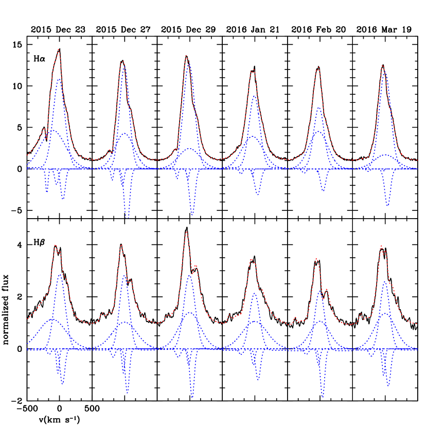
Figure 12: H$\alpha$ and H$\beta$ continuum-normalized profile (black). In red we show the fit to the profile, obtained by adding multiple Gaussians (blue dotted lines, where a constant c=1 was subtracted from the fit for better visualization). The date of the observation is reported as well.

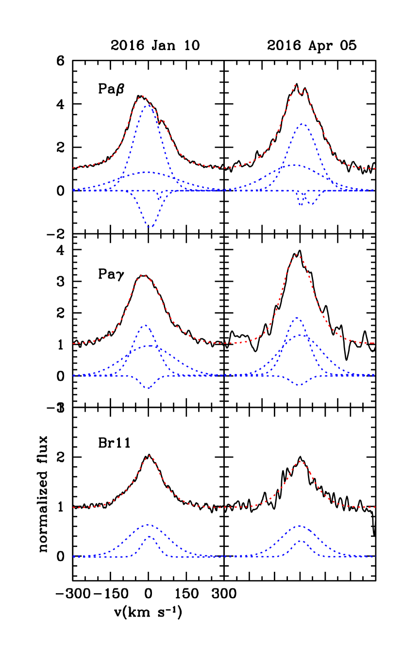
Figure 13: Continuum-normalized profile of the brightest Paschen and Brackett lines (black). In red we show the fit to the profile, obtained by adding multiple Gaussians (blue dotted lines, where a constant c=1 was subtracted fromthe fit for better visualization). The date of the observation is reported as well.

Fits of selected lines are shown in Figures 12, 13 and in Table 10. Although five Gaussians are required to fit the H$\alpha$ and H$\beta$ profiles, most of the observed flux is accounted for by two main components. These are a narrow component, slightly blue-shifted of a few km s^-1 with a FWHM close to 200 km s^-1, and a broad component, centered close to the rest velocity, with extended wings wider than $\pm$ 500 km s^-1. Variable self-absorption features are recognizable on both sides of the profile, and the red-shifted feature (centered at $\sim$ +40 km s^-1) is the most prominent. An outflowing wind is shown by a P Cyg-like absorption (e.g. Edwards et al. 2003) at v $\sim$ $-$200 km s^-1, clearly visible in the H$\alpha$ profile on 2015 December 23. In contrast to the observations of Herbig (2008), who noted a link between the source activity and a P Cyg absorption, our spectra reveal a more complex situation, since the P Cyg clearly faded in a few days while the outburst was in a stable and peak phase. Similarly, the H$\beta$, although not presenting a prominent P Cyg-like feature, exhibits a pronounced blue wing in the spectrum of December 23 that disappears in the following days. Such sudden and brief wind enhancement is also shown by the shift of the broad velocity component peak of about $-$100 km s^-1 (see Table 10).

In contrast to the Balmer lines, other H I  lines present more symmetric profiles (Figure 13) composed of a narrow and a broad component, which tend to become narrower with the increase of the number of the upper energy level (n_up, Figure 14). First, this might be explained in the framework of a temperature and density gradient in the emitting gas. For example, according to the Kwan and Fischer models of the Balmer decrements (Figure  10), flux ratios involving lines with higher n_up increase with increasing temperature and density. Since this hot and dense gas is probably only a portion of the total hydrogen emitting gas, we expect that it is characterized by a smaller range of velocity than the gas probed by lines with lower n_up (e.g. H$\alpha$). Other possible causes for differential line broadening may be Stark and van der Waals effects, which may produce significant high-velocity emission in H$\alpha$ and, to a lesser extent, in other Balmer lines (Muzerolle, Calvet, & Hartmann 2001). We cannot exclude, however, that the observed behavior is, at least partially, a consequence of other causes. In particular, the FHWM of the narrow component of the brightest lines might be overestimated as the profiles can be saturated or even self-absorbed because of opacity effects. Conversely, in the broad component, the FWHM of the faintest lines may be underestimated because the wings are confused inside the continuum fluctuation.

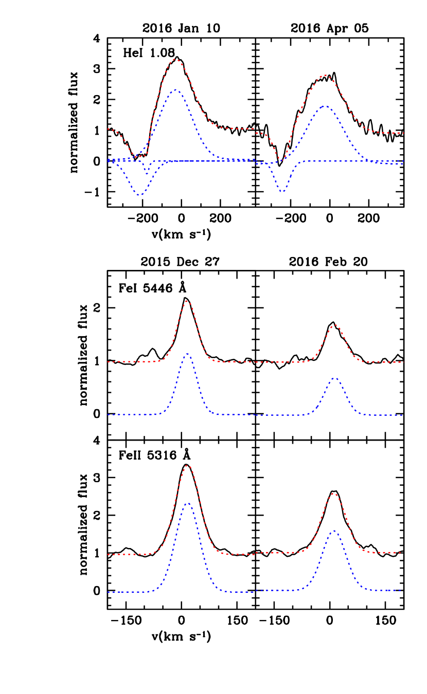
Figure 15: Top panel: Continuum-normalized He I  1.08 $\mu$m profile (black). In red we show the fit to the profile, obtained by adding multiple Gaussians (blue dotted lines, where a constant c=1 was subtracted from the fit for a better visualization). The date of the observation is reported, as well. Bottom panels: the same as in the top panel for Fe I  5446 Å  and Fe II  5316 Å  taken as examples of the metallic lines. These profiles are shown on two dates that are representative of the outburst evolution.

In Figure 15, top panel, we show the profile of the He I  1.08 $\mu$m. The line can be deconvolved into two main Gaussians in the two observation dates in 2016 January and April. The main component is in emission, with the center a v $\sim$ $-$25 km s^-1 and FHWM $\sim$ 200 km s^-1, namely similar to the parameters of the narrow component of the H$\alpha$ line. An ionized wind is shown by a pronounced P Cyg-like absorption (v_peak $\sim$ $-$200 km s^-1 ), which, differently from the H I  lines, is well visible until the end of the peak phase.

Fe I  and Fe II  lines are well fitted with a single Gaussian centered close to the rest velocity with width $<$ 100 km s^-1 (Figure 15, bottom panels). This allows us to rule out both that they form in the stellar photosphere (the FHWM should be of only a few km s^-1) and that they originate from the same gas as the H I  and the He I  lines. Rather, as already hypothesized in Section 3.2.4, they might arise at the base of the accretion columns close to the disk surface, where the gas is mostly neutral and still relatively slow. Given the large number of Fe I  and Fe II  lines, we have investigated whether or not a difference exists between their average width ($<$FHWM$>$). We find that Fe I  lines have $<$FHWM$>$ = 64$\pm$8 km s^-1 against a $<$FHWM$>$ of Fe II  lines of 85$\pm$15 km s^-1. For both species, the $<$FHWM$>$ evolves with time, and the maximum value is reached on 2016 January, when the $<$FHWM$>$ was 71$\pm$11 km s^-1 and 109$\pm$33 km s^-1 for the Fe I  and Fe II  lines, respectively.

4 Summary

We have presented a photometric and spectroscopic study of the recent outburst of the classical EXor source V1118 Ori, after following its evolution from the rising to the peak and declining phase. The derived parameters have been meaningfully compared with those already measured in quiescence at a similar level of sensitivity. Our main results are summarized in Table 11, and can be listed as follows:

• The 2015-2016 outburst of V1118 Ori is the sixth well-documented event in the past $\sim$ 40 years. The source brightness suddenly increased around 2015 September, reaching its peak around 2016 January and starting to decline around 2016 April. Magnitudes close to the quiescence values have been measured since 2016 September.

• The 2015 outburst has occurred after a relatively long period of quiescence (about 10 years), while the events of the past three decades have shown a roughly regular recurrence of 6$-$8 years. This circumstance does not support the theory that periodic phenomena are the cause of the outburst triggering.

• A blueing effect is clearly recognizable in the [$V-R$] vs. [$R-I$] diagram. In agreement with previous works on the same object and on EXors in general, we interpret it as the signature of the accretion burst.

• Mass accretion rates were computed for all the outburst phases and compared with the quiescence value. We estimate that $\dot{M}_{acc}$  increases by about two orders of magnitude from the quiescence to the outburst peak, specifically from 0.3$-$2.0 10^-8 M_⊙ yr^-1  to 0.2-1.9 10^-6 M_⊙ yr^-1. A comparable increase occurs in the hydrogen density, from $\sim$ 2 10⁹ cm^-3 to $\sim$ 4 10¹¹ cm^-3. The gas temperature is not well constrained, but we can place a lower limit of $\sim$ 8000 $-$ 9000 K during outburst.

• Optical/near-infrared outburst spectra are rich in metallic lines, mainly coming from neutral atoms typical of M-type stars. Our analysis suggests that these lines originate close to the disk surface, in regions sufficiently shielded from UV radiation to prevent their ionization. This view is confirmed by the relatively narrow profiles ($\sim$ 60 km s^-1) of the Fe I  lines.

• H$\alpha$ and H$\beta$ lines present complex profiles, with wings extending up to $\pm$ 500 km s^-1, while profiles of other H I  lines are more symmetric and tend to become narrower for increasing n_up. We tentatively explain such behavior considering that lines at higher energy originate preferentially in the warmest and densest gas component. Stark and van der Waals effects may also play a role.

• An outflowing activity is demonstrated by a P Cyg-like absorption in the H$\alpha$, H$\beta$, and He I  1.08 $\mu$m profiles. While this feature disappears in the H I line profiles on a timescale of a week, it is more stable in the highly ionized gas, being recognizable for at least four months in the He I  profile.
  

  As a final consideration, we remark that our study has taken benefited greatly from the observations of the quiescence phase, since this allowed us to define the zeroes of the physical parameters. Therefore systematic observations of EXors also during quiescence (like our EXORCISM monitoring program, which has been ongoing since several years), are of great help in order to place the outburst phenomenology in a comparative and statistical context.

Appendix A Appendix A

In Table 12 we give the list of the optical, unblended lines detected with the echelle at the 1.82 Asiago telescope ($\Re$ $\sim$ 20 000).

Appendix B Appendix B

In Table 13 we give the list of the near-infrared, unblended lines detected with GIANO at the TNG telescope ( $\Re$ $\sim$ 50 000).

Appendix C Acknowledgements

The authors sincerely thank John Kwan for providing the predictions of his local line excitation models. CFM acknowledges an ESA Research Fellowship. This work is based on observations made with different instruments:[1] the Large Binocular Telescope (LBT). The LBT is an international collaboration among institutions in the United States, Italy and Germany. LBT Corporation partners are: The University of Arizona on behalf of the Arizona university system; Istituto Nazionale di Astrofisica, Italy; LBT Beteiligungsgesellschaft, Germany, representing the Max-Planck Society, the Astrophysical Institute Potsdam, and Heidelberg University; The Ohio State University, and The Research Corporation, on behalf of The University of Notre Dame, University of Minnesota and University of Virginia; [2] the Asiago ANS Collaboration telescopes operated under the responsability of the INAF-Osservatorio Astronomico di Padova (OAPd); [3] the AZT-24 IR telescope at Campo Imperatore (L’Aquila - Italy) operated by INAF-Osservatorio Astronomico di Roma (OAR); [4] the TNG telescope at La Palma (Spain) operated by INAF. We acknowledge the observers that contribute to the AAVSO International Database.

Figure 4: Optical low-resolution spectra of V1118 Ori taken with the 1.22m Asiago telescope during the peak phase. For a better visualization a constant was added to the flux density. Main emission lines are labeled.

Table 1: Optical photometry

Date	MJD	B	V	Rc	Ic	Tel.
	(days)	(mag)
2016 Jan 06	57393.412	14.59	13.83	13.24	12.51	036
2016 Jan 13	57400.420	14.59	13.92	13.28	12.56	036
2016 Jan 14	57401.371	14.66	14.08	13.39	12.68	157
2016 Jan 16	57403.251	14.51	13.89	13.18	12.53	157
2016 Jan 17	57404.352	14.79	14.01	13.38	12.63	036
2016 Jan 20	57407.357	14.81	14.14	13.51	12.76	036
2016 Jan 26	57413.230	14.43	13.75	13.09	12.41	157
2016 Jan 26	57413.245	14.51	13.78	13.18	12.43	036
2016 Feb 01	57419.427	-	14.08	13.48	12.74	036
2016 Feb 06	57424.234	14.96	14.28	13.52	12.83	157
2016 Feb 06	57424.253	14.89	14.26	13.56	12.82	036
2016 Feb 12	57430.236	14.89	14.32	13.63	12.95	157
2016 Feb 19	57437.242	14.97	14.49	13.86	13.09	157
2016 Feb 20	57438.243	14.84	14.17	13.40	12.74	157
2016 Feb 21	57439.296	14.53	13.72	13.06	12.47	036
2016 Feb 21	57439.312	14.26	13.74	13.17	12.49	157
2016 Feb 21	57439.362	-	13.71	-	12.46	036
2016 Feb 22	57440.259	14.59	14.09	13.20	12.55	157
2016 Feb 22	57440.364	14.45	13.75	12.97	12.42	036
2016 Feb 24	57442.249	14.46	13.85	13.14	12.48	157
2016 Mar 02	57449.244	14.72	13.98	13.36	12.63	157
2016 Mar 02	57449.319	14.59	14.00	13.38	12.61	036
2016 Mar 15	57462.257	14.18	13.53	12.84	12.17	157
2016 Mar 15	57462.281	14.23	13.58	12.88	12.19	036
2016 Mar 18	57465.256	14.28	13.56	12.93	12.26	157
2016 Mar 19	57466.258	14.38	13.72	13.01	12.29	157
2016 Mar 19	57466.316	14.43	13.67	13.00	12.30	036
2016 Mar 24	57471.301	14.55	13.79	-	12.41	036
2016 Mar 30	57477.284	14.42	13.75	13.08	12.39	157
2016 Apr 12	57490.279	14.58	13.80	13.06	12.36	157
2016 Apr 16	57494.285	14.65	13.84	13.14	12.42	157
2016 Aug 25	57625.622	-	14.50	-	13.59	036
2016 Sep 06	57637.619	15.97	15.64	14.94	14.16	157
2016 Sep 09	57640.637	16.51	16.10	15.28	14.31	157
2016 Oct 27	57688.675	-	15.99	-	14.35	036
2016 Oct 29	57690.455	16.42	16.34	15.36	14.45	157
2016 Nov 11	57699.466	16.81	16.54	15.41	14.64	157
2016 Nov 30	57723.435	16.97	16.41	15.52	14.64	157
2016 Dec 05	57728.473	-	16.28	-	14.43	036

Note. — Typical errors are smaller than 0.02 mag.

Table 2: Near-IR photometry.

Date	MJD	J	H	K
	(days)	(mag)
2015 Dec 18	57374.474	11.34	10.63	9.83
2016 Feb 02	57442.356	11.45	10.69	9.89
2016 Feb 24	57442.366	11.46	10.68	-
2016 Sep 21	57652.574	12.49	11.41	10.57
2016 Sep 23	57654.600	12.53	11.47	10.71
2016 Sep 25	57656.616	12.58	11.51	10.76
2016 Sep 27	57658.612	12.56	11.51	10.74
2016 Sep 28	57659.597	12.55	11.51	10.75
2016 Sep 30	57661.580	12.46	11.41	10.62
2016 Oct 01	57662.667	12.57	11.50	10.67
2016 Oct 29	57690.548	12.42	11.33	10.67
2016 Oct 31	57692.598	12.46	11.41	10.65
2016 Nov 02	57694.504	12.47	11.39	10.61

Note. — Typical errors are smaller than 0.03 mag.

Table 3: WISE photometry.

Date	MJD	[3.4]	[4.6]	[12]
	(days)	(mag$\pm$ $\Delta$mag)
2010 Aug 03	55263	9.84$\pm$0.03	9.01$\pm$0.02	6.87$\pm$0.06
2010 Sep 09	55454	9.95$\pm$0.05	9.10$\pm$0.06	6.96$\pm$0.06
2014 Mar 08	56724	9.93$\pm$0.03	9.14$\pm$0.03	-
2014 Mar 11	56727	10.04$\pm$0.17	9.21$\pm$0.09	-
2014 Mar 12	56728	9.94$\pm$0.02	9.12$\pm$0.03	-
2014 Sep 15	56915	9.95$\pm$0.03	9.13$\pm$0.03	-
2014 Sep 19	56919	9.96$\pm$0.03	9.12$\pm$0.03	-
2015 Mar 06	57087	9.94$\pm$0.03	9.13$\pm$0.02	-
2015 Sep 16	57281	8.98$\pm$0.06	8.14$\pm$0.06	-

Table 4: Journal of spectroscopic observations.

Date	MJD	Telescope/Instrument	$\Delta\lambda$	$\Re$	rms	Exp time
			(Å)		($10^{-16}$ erg s-1 cm-2 Å-1)	(s)
2015 Dec 23	57379	1.22m/B&C	3300-8050	2400	7-12	1800
2015 Dec 23	57379	1.82m/ECH	3600-7300	20 000	7-20	1800
2015 Dec 27	57383	1.22m/B&C	3300-8050	2400	4-7	3600
2015 Dec 27	57383	1.82m/ECH	3600-7300	20 000	7-25	1800
2015 Dec 29	57385	1.82m/ECH	3600-7300	20 000	4-13	3600
2016 Jan 10	57397	TNG/GIANO	9500-24 500	50 000	-	3000
2016 Jan 12	57399	LBT/MODS	3200-9500	1500	0.9-1.2	1500
2016 Jan 21	57408	1.82m/ECH	3600-7300	20 000	15-38	3600
2016 Jan 21	57408	1.22m/B&C	3300-8050	2400	3-6	3600
2016 Jan 25	57412	LBT/LUCI2	10 000-24 000	1000	0.7-1.6	1200
2016 Jan 26	57413	LBT/MODS	3200-9500	1500	0.9-1.1	1500
2016 Jan 31	57418	LBT/MODS	3200-9500	1500	0.7-1.0	1500
2016 Feb 05	57423	1.22m/B&C	3300-8050	2400	4-7	3600
2016 Feb 20	57438	1.22m/B&C	3300-8050	2400	2-6	5400
2016 Feb 20	57438	1.82m/ECH	3600-7300	20 000	12-41	3600
2016 Mar 02	57449	LBT/LUCI2	10 000-24 000	1000	1.1-2.2	1200
2016 Mar 13	57460	1.22m/B&C	3300-8050	2400	10-20	900
2016 Mar 19	57466	1.82m/ECH	3600-7300	20 000	12-42	1800
2016 Mar 19	57466	1.22m/B&C	3300-8050	2400	8-20	2400
2016 Apr 05	57483	TNG/GIANO	9500-24 500	50 000	-	3000
2016 Oct 04	57665	LBT/LUCI2	10 000-24 000	1300	0.7-2.0	1200
2016 Dec 04	57726	LBT/MODS	3250-9500	1500	0.7-1.0	1500

Table 5: Fluxes of main lines detected with LBT/MODS.

		2016 Jan 12	2016 Jan 26	2016 Jan 31	2016 Dec 04
Line	$\lambda_{air}$	Flux$\pm\Delta$ Flux
	(Å)	(10-15 erg s-1 cm-2)
H15	3711.97	10.5$\pm$1.8	-	15.8$\pm$2.0	-
H14	3721.94	14.3$\pm$1.8	9.9$\pm$0.9	18.8$\pm$2.0	-
H13	3734.37	18.7$\pm$1.8	12.2$\pm$1.1	23.9$\pm$2.0	-
H12	3750.15	21.7$\pm$1.8	12.7$\pm$1.1	25.5$\pm$2.0	2.1$\pm$0.7
H11	3770.63	20.4$\pm$1.8	11.6$\pm$1.1	22.4$\pm$2.0	3.1$\pm$0.7
H10	3797.90	21.9$\pm$1.8	10.9$\pm$1.1	31.6$\pm$2.0	4.9$\pm$0.7
H9	3835.38	32.8$\pm$1.8	10.7$\pm$1.1	32.5$\pm$2.0	6.3$\pm$0.7
H8	3889.05	29.6$\pm$1.8	10.3$\pm$0.9	33.0$\pm$2.0	9.5$\pm$0.7
CaII H	3933.66	105.92$\pm$1.7	73.3$\pm$1.0	170.3$\pm$2.0	3.5$\pm$0.7
CaII K + H7	3968.45/3970.07	99.2$\pm$1.7	55.3$\pm$1.0	152.4$\pm$2.0	14.1$\pm$0.7
HeI	4026.19	9.2$\pm$1.7	6.5$\pm$1.0	9.8$\pm$2.0	-
H$\delta$	4101.73	50.4$\pm$1.7	28.3$\pm$1.0	75.7$\pm$2.0	17.15$\pm$0.4
H$\gamma$	4340.46	71.9$\pm$1.7	42.0$\pm$1.0	96.8$\pm$2.0	20.3$\pm$0.4
H$\beta$	4861.32	186.11$\pm$1.7	112.6$\pm$1.0	231.3$\pm$2.0	31.1$\pm$0.2
HeI	5015.68	16.18$\pm$1.7	12.0$\pm$1.0	14.1$\pm$2.0	1.4$\pm$0.2
Mg I	5168.76/5174.12	27.8$\pm$1.7	36.2$\pm$1.7	20.2$\pm$1.0	-
Mg I	5185.05	7.3$\pm$1.7	10.2$\pm$1.7	5.4$\pm$1.0	-
HeI	5875.6	27.1$\pm$1.8	13.5$\pm$1.1	29.5$\pm$2.0	3.5$\pm$0.2
$[\rm{OI}]$	6300.30	15.5$\pm$1.8	9.5$\pm$1.2	11.7$\pm$2.0	15.75$\pm$0.2
H$\alpha$	6562.80	1546.8$\pm$2.0	765.0$\pm$1.2	1635.5$\pm$2.0	149.4$\pm$0.2
HeI	6678.15	23.9$\pm$2.0	14.5$\pm$1.2	23.2$\pm$2.0	2.8$\pm$0.2
HeI	7065.2	15.8$\pm$2.0	10.3$\pm$1.2	14.3$\pm$2.0	-
OI	8446.5	59.6$\pm$2.0	34.4$\pm$1.1	51.9$\pm$2.0	4.5$\pm$0.2
CaII	8498.03	572.8$\pm$2.0	372.3$\pm$1.0	526.8$\pm$2.0	9.1$\pm$0.2
CaII	8542.09	670.5$\pm$2.0	430.7$\pm$1.0	636.5$\pm$2.0	8.0$\pm$0.2
CaII	8662.14	584.9$\pm$2.0	370.6$\pm$1.0	546.2$\pm$2.0	8.4$\pm$0.2
Pa12	8750.47	97.0$\pm$2.0	64.3$\pm$1.3	75.4$\pm$2.0	-
Pa9	9229.01	183.7$\pm$2.0	89.3$\pm$1.3	144.5$\pm$2.0	5.2$\pm$0.2

Table 6: Fluxes of lines detected with the Asiago telescopes.

Date	Flux${}^{a}\pm\Delta$ Flux (10-15 erg s-1 cm-2)
	H$\alpha^{b}$	H$\beta$	H$\gamma$	H$\delta$	CaII H
2015 Dec 23	1259$\pm$19	162$\pm$18	71$\pm$22	54$\pm$20	89$\pm$20
2015 Dec 27	1070$\pm$16	142$\pm$18	69$\pm$20	51$\pm$20	68$\pm$25
2015 Dec 29c	1291$\pm$18	172$\pm$19	74$\pm$20	71$\pm$20	74$\pm$20
2016 Jan 21	1129$\pm$19	197$\pm$20	97$\pm$24	50$\pm$20	84$\pm$20
2016 Feb 05d	1076$\pm$12	177$\pm$12	58$\pm$17	-	-
2016 Feb 20	1051$\pm$18	118$\pm$18	64$\pm$20	-	86$\pm$25
2016 Mar 13d	1110$\pm$30	189$\pm$30	63$\pm$23	-	-
2016 Mar 19	1056$\pm$18	115$\pm$18	52$\pm$20	-	-

Table 7: Fluxes of main lines detected with LUCI2.

		2016 Jan 25	2016 Mar 02	2016 Oct 04
Line	$\lambda_{air}$	Flux$\pm\Delta$ Flux
	(Å)	(10-15 erg s-1 cm-2)
Pa$\delta$	10049.37	238.1$\pm$2.0	181.5$\pm$2.0	40.0$\pm$2.0
HeI	10830.3	(-32.2) 79.8$\pm$2.0	(-18.0) 113.8$\pm$2.0	(-3.5) 7.2 $\pm$0.3
Pa$\gamma$	10938.09	274.9$\pm$2.0	196.2$\pm$2.0	65.3$\pm$1.0
NaI	11406.90	27.9 $\pm$3.0	32.6$\pm$3.0	-
Pa$\beta$	12818.08	362.5$\pm$2.0	282.8$\pm$2.0	71.8$\pm$1.0
MgI	15029/15051	75.6$\pm$4.0	52.3$\pm$3.0	-
Br19	15264.71	26.8$\pm$4.0	23.4$\pm$3.0	-
Br18	15345.98	27.7$\pm$4.0	26.8$\pm$3.0	-
Br17	15443.14	34.3$\pm$4.0	34.0$\pm$3.0	-
Br16	15560.70	31.2$\pm$4.0	36.8$\pm$3.0	-
Br15	15704.95	41.0$\pm$4.0	37.4$\pm$3.0	-
Br14+OI	15885/15892	111.4$\pm$4.0	97.3$\pm$3.0	-
Br13	16113.71	51.1$\pm$4.0	47.6$\pm$3.0	-
Br12	16411.67	72.0$\pm$4.0	72.0$\pm$3.0	-
Br11	16811.11	73.4$\pm$4.0	75.1$\pm$3.0	15.6$\pm$3.0
Br10	17366.85	84.9$\pm$4.0	80.0$\pm$3.0	10.1$\pm$3.0
H2 1-0 S(1)	-	-	-	3.9$\pm$0.7
Br$\gamma$	21655.29	83.8$\pm$4.0	75.6$\pm$3.0	15.5$\pm$0.7
NaI	22062.4	17.5$\pm$4.0	10.0$\pm$3.0	-
NaI	22089.7	10.9$\pm$4.0	9.9$\pm$3.0	-
CO 2-0	22943	185.1$\pm$10.0	140.8$\pm$10.0	-
CO 3-1	23235	161.7$\pm$10.0	117.9$\pm$10.0	-

Table 8: Mass accretion rate.

Phase	$\dot{M}_{acc}$ (M⊙ yr-1)a
	C-1.5	C-2.9	L-1.5	L-2.9
Quiescenceb	3.1$\pm$1.0 10-9	2.0$\pm$0.7 10-8	3.5$\pm$2.5 10-9	1.6$\pm$1.1 10-8
Risingc	1.1$\pm$0.4 10-7	6.8$\pm$2.4 10-7	4.2$\pm$0.8 10-8	3.1$\pm$0.5 10-7
Peakd	3.2$\pm$1.1 10-7	1.9$\pm$0.7 10-6	2.0$\pm$1.0 10-7	9.6$\pm$3.1 10-7
Declininge	-	-	8.0$\pm$2.2 10-8	1.4$\pm$0.5 10-7
Post-outburstf	3.0$\pm$0.4 10-8	6.4$\pm$0.4 10-8	2.6$\pm$0.9 10-8	1.8$\pm$0.8 10-7

Table 9: Statistics^a of the optical permitted lines.

Element	IPb	V1118 Ori		EX Lup
		max(Eup)b	Nlines	max(Eup)b	Nlines
Li I	5.39	1.8	2	-	-
Na I	5.13	2.1	2	4.9	3
Mg I	7.64	5.1	1	7.6	10
Si I	8.15	5.1	1	7.5	7
Si II	16.34	10.1	2	14.8	6
Ca I	6.11	4.5	15	5.7	27
Ca II	11.87	3.1	2	10.0	3
Ti I	6.82	6.0	15	3.9	6
Ti II	13.57	5.6	21	5.6	43
V I	6.74	5.4	10	4.7	4
Cr I	6.76	5.0	11	5.0	31
Cr II	16.49	6.8	5	6.8	12
Fe I	7.87	6.7	112	7.2	$>$ 400
Fe II	16.18	5.9	39	8.2	$\sim$ 70
Co I	7.86	4.0	2	4.2	9
Ni I	7.63	4.1	4	6.1	17

Table 10: Parameters of the main Gaussians fitting the H I  lines. Units are km s^-1.

Date	Narrow		Broad		P Cygni
	Center	FWHM	Center	FWHM	Center	FWHM
H$\alpha$
2015 Dec 23	-9	209	-101	449	-195	42
2015 Dec 27	-4	172	-3	339	-191	41
2015 Dec 29	-12	203	-7	387	-195	38
2016 Jan 21	-8	192	-37	383	-213	60
2016 Feb 20	-17	185	-25	341	-243	71
2016 Mar 19	-3	205	1	402	-259	61
H$\beta$
2015 Dec 23	3	197	-111	488	-159	65
2015 Dec 27	-4	174	-1	434	-176	69
2015 Dec 29	-5	203	-1	387	-177	83
2016 Jan 21	-5	182	-2	451	-212	83
2016 Feb 20	-5	174	-2	350	-212	83
2016 Mar 19	-5	172	-2	373	-212	83
Pa$\beta$
2016 Jan 10	-3	112	-5	282	-	-
2016 Apr 05	10	109	-23	247	-	-
Pa$\gamma$
2016 Jan 10	-14	112	2	234	-	-
2016 Apr 05	-12	109	2	199	-	-
Br10
2016 Jan 10	3	81	6	177	-	-
Br11
2016 Jan 10	5	72	-2	183	-	-
2016 Apr 05	4	78	-1	171	-	-
Br12
2016 Jan 10	4	86	3	273a	-	-
2016 Apr 05	4	99	3	264a	-	-
Br13
2016 Jan 10	6	72	-4	192	-	-

Table 11: 2015-2016 outburst parameters of V1118 Ori.

Parameter	Value
$\Delta V^{a}$	4 mag
Duration	$\sim$ 1 year
Rising velocity	$\lesssim$ 0.008 mag/day
Declining velocity	$\sim$ 0.015 mag/day
Periodicity	hints
$<\Delta$[V-R]$>^{a}$	$\sim$ 0.4 mag
$<\Delta$[H-K]$>^{a}$	$\sim$ 0.0 mag
Peak $\dot{M}_{acc}$	0.1-1.2 10-6 M⊙ yr-1
Electron density	$\sim$ 4 1011 cm-3
Metals	mostly neutrals
$<$FHWM$>$ neutrals	$<$ 100 km s-1
$<$FHWM$>$ H I  lines	up to 450 km s-1
Wind?	yes, variable P Cyg

Table 12: Lines observed with the REOSC Echelle at the 1.82m Asiago telescope, grouped according to element

Line	$\lambda_{air}$	Aij	Eup
	(Å)	(s-1)	(eV)
H$\delta$	4101.73	9.72e+05	13.220
H$\gamma$	4340.46	2.53e+06	13.054
H$\beta$	4861.28	8.41e+06	12.748
H$\alpha$	6562.57	4.41e+07	12.087
He I	4471.47	2.47e+07	23.736
He I	5875.6	7.09e+07	23.073
He I	6678.15	6.38e+07	23.074
He I	7065.19	1.55e+07	22.718
Li I	6707.76	3.70e+07	1.847
Li I	6707.91	3.70e+07	1.847
O I	6300.30	5.63e-03	1.967
O I	6363.77	1.82e-03	1.967
NaI D	5889.95	6.24e+07	2.104
NaI D	5895.92	6.22e+07	2.102
Mg I	5183.60	5.61e+07	5.107
Si I	3905.52	1.39e+07	5.082
Si II	6347.10	6.11e+07	10.073
Si II	6371.36	6.05e+07	10.066
Ca I	4226.73	2.19e+08	2.932
Ca I	4302.53	1.43e+08	4.779
Ca I	4434.96	6.37e+07	4.680
Ca I	4454.77	8.38e+07	4.681
Ca I	5602.85	1.78e+07	4.735
Ca I	6102.72	9.53e+06	3.910
Ca I	6122.22	2.85e+07	3.910
Ca I	6162.17	4.74e+07	3.910
Ca I	6169.06	8.12e+06	4.532
Ca I	6439.07	4.26e+07	4.450
Ca I	6449.81	6.68e+06	4.443
Ca I	6462.57	3.75e+07	4.440
Ca I	6471.66	4.66e+06	4.440
Ca I	6717.69	1.08e+07	4.554
Ca I	7148.15	3.90e+07	4.443
CaII H	3933.66	1.40e+08	3.150
CaII K	3968.46	1.36e+08	3.123
Ti I	4783.30	6.20e+04	3.41
Ti I	4899.91	-	4.41
Ti I]	4934.58	-	4.84
Ti I	5006.99	-	5.69
Ti I	5136.64	-	5.96
Ti I	5153.48	-	5.69
Ti I	5265.71	-	4.48
Ti I/V I	5473.50/5473.59	-	4.59/4.62
Ti I	5527.61	-	4.67
Ti I	5711.89	-	4.47
Ti I	6359.20	-	4.10
Ti I	6583.64	-	5.20
Ti I	6738.33	-	5.30
Ti I	6743.12	6.90e+05	2.74
Ti I	6772.66	-	6.05
Ti II	4294.10	4.70e+06	3.97
Ti II	4307.86	4.60e+06	4.04
Ti II	4314.97	1.30e+07	4.03
Ti II	4320.96	2.40e+06	4.03
Ti II	4394.05	2.20e+06	4.04
Ti II	4399.77	3.10e+06	4.05
Ti II	4417.72	2.10e+06	3.97
Ti II	4443.79	1.10e+07	3.87
Ti II	4450.49	2.00e+06	3.87
Ti II	4464.45	7.00e+05	3.94
Ti II	4468.50	1.00e+07	3.90
Ti II	4501.27	9.80e+06	3.86
Ti II	4563.77	8.80e+06	3.94
Ti II	4571.98	1.20e+07	4.28
Ti II/Fe II	4629.28/.34	2.20e+05/1.30e+05	3.86/5.48
Ti II	4779.98	6.20e+06	4.64
Ti II	4798.52	1.80e+05	3.66
Ti II	4805.08	1.10e+07	4.64
Ti II	4911.19	3.20e+07	5.65
Ti II	5129.15	1.00e+06	4.31
Ti II	5188.68	2.50e+06	3.97
Ti II	5336.77	5.80e+05	3.90
Ti II	5381.01	3.20e+05	3.87
V I	3912.88	3.30e+06	4.23
V I	3914.39	-	5.44
V I	4405.01	3.40e+05	3.09
V I	4753.93	1.50e+07	4.68
V I	5410.46	-	4.86
V I]	5413.36	-	2.56
V I	5415.24	3.10e+07	4.66
V I	5463.34	-	4.85
V I	5489.93	2.9e+07	4.63
V I	5762.73/.83	-/-	4.72/4.28
V I	7005.45	-	3.89
Cr I	4254.33	3.15e+07	2.91
Cr I	4580.04	2.40e+06	3.65
Cr I	4903.22	7.40e+06	5.07
Cr I	5204.51	5.09e+07	3.32
Cr I	5206.04	5.14e+07	3.32
Cr I	5208.44	5.06e+07	3.32
Cr I	5247.57	1.90e+06	3.32
Cr I	5298.27	3.30e+06	3.32
Cr I	5345.81	4.90e+06	3.32
Cr I	5348.61	1.70e+06	3.32
Cr I	5409.77	6.20e+06	3.32
Cr II	4558.66	8.80e+06	6.79
Cr II	4634.07	8.90e+06	6.75
Cr II	4824.13	1.70e+06	6.44
Cr II	4848.23	2.60e+06	6.42
Cr II	4876.47	1.60e+06	6.41
Fe I	4063.59	6.80e+07	4.61
Fe I	4118.54	5.80e+07	6.58
Fe I	4123.72/.76	2.79/4.50e+05/	6.00/5.6
Fe I	4132.05	1.20e+07	4.61
Fe I	4154.49	4.96e+07	5.82
Fe I	4173.31	2.10e+06	5.82
Fe I	4191.43	3.19e+07	5.43
Fe I	4198.63	2.46e+07	6.37
Fe I	4202.02	8.22e+06	4.43
Fe I	4216.18	1.84e+04	2.93
Fe I	4233.60	2.33e+07	5.41
Fe I	4250.11/.79	2.63/1.00e+07	5.39/4.47
Fe I	4260.47	4.67e+07	6.31/5.3
Fe I	4271.15/.76	2.26/2.28e+07	5.35/4.3
Fe I	4282.40	1.10e+07	5.07
Fe I	4289.91	2.69e+06	6.29
Fe I	4324.94	1.63e+04	5.06
Fe I	4375.98	2.96e+05	5.8
Fe I	4415.12	1.19e+07	4.42
Fe I	4427.29	6.87e+06	6.45
Fe I	4442.34	3.76e+06	4.99
Fe I	4443.19	1.26e+07	5.64
Fe I	4447.71	5.11e+06	5.01
Fe I	4459.11	2.52e+06	4.96
Fe I	4461.65	2.95e+04	2.87
Fe I	4466.55	1.58e+07	5.61
Fe I	4476.01	1.36e+07	5.61
Fe I	4482.25	1.95e+06	4.98
Fe I	4489.73	1.19e+04	2.88
Fe I	4494.56	3.45e+06	4.95
Fe I	4528.61	5.44e+06	4.91
Fe I/Ti II	4533.96/.97	2.21e+04/9.20e+06	5.68/3.97
Fe I	4583.72	5.90e+05	5.82
Fe I	4602.94	1.48e+05	4.18
Fe I/Cr II	4618.76/.80	1.60e+05/6.1e+06	5.63/6.76
Fe I	4654.60/.63	9.98e+06/9.33e+05	6.26/5.87
Fe I	4667.45	4.18e+06	6.25
Fe I	4678.84	2.23e+07	6.25
Fe I	4702.91	3.92e+04	5.87
Fe I	4736.77	4.90e+06	5.83
Fe I	4786.80	1.21e+06	5.61
Fe I	4871.31	3.22e+07	5.41
Fe I	4877.60	5.79e+04	5.53
Fe I	4891.49	4.10e+07	5.39
Fe I	4918.99	2.31e+07	5.39
Fe I	4920.50	4.90e+07	5.35
Fe I	4939.24	5.78e+06	6.66
Fe I	4957.60	5.53e+07	5.31
Fe I	4985.25	2.96e+07	6.41
Fe I	4994.12	3.18e+04	3.39
Fe I	5006.11	7.28e+06	5.31
Fe I	5012.06	5.50e+04	3.33
Fe I	5030.77	2.60e+04	5.70
Fe I	5041.07	2.15e+05	3.42
Fe I	5049.81	2.31e+06	4.73
Fe I	5051.63	4.65e+04	3.37
Fe I	5064.95	2.88e+06	6.70
Fe I	5068.76	3.37e+06	5.39
Fe I	5079.22/.74	7.39e+05/5.19e+04	4.64/3.43
Fe I	5083.33	4.06e+04	3.40
Fe I	5098.57/.69	6.08e+05/2.97e+05	6.36/4.61
Fe I	5107.64	1.95e+05	3.98
Fe I	5110.35	1.26e+06	6.0
Fe I	5123.72	7.24e+04	3.4
Fe I	5127.36	1.14e+04	3.3
Fe I	5139.25	1.13e+07	5.4
Fe I	5141.73	7.62e+05	4.8
Fe I	5150.83	3.10e+04	3.4
Fe I	5167.49	2.00e+06	3.88
Fe I	5171.60	4.46e+05	3.8
Fe I	5191.45	2.97e+07	5.43
Fe I	5194.94	2.87e+05	3.94
Fe I	5202.25	5.14e+06	6.64
Fe I	5216.27	3.47e+05	3.98
Fe I	5227.15/.19	1.40e+06/4.23e+06	4.80/3.93
Fe I	5232.94	2.57e+07	5.31
Fe I	5250.64	3.10e+05	4.56
Fe I	5254.97	2.15e+04	6.65
Fe I	5270.35	2.50e+06	3.96
Fe I	5302.30	1.17e+06	5.62
Fe I	5307.36	3.49e+04	3.94
Fe I	5324.17	2.74e+07	5.54
Fe I	5328.03	1.15e+06	3.24
Fe I	5332.89	3.00e+04	3.88
Fe I	5341.02	4.10e+05	3.93
Fe I	5371.48	1.05e+06	3.27
Fe I	5383.36	5.60e+07	6.61
Fe I	5393.16	6.34e+06	5.54
Fe I	5397.12	2.59e+05	3.21
Fe I	5405.77	1.09e+06	3.28
Fe I	5429.69	4.27e+05	3.24
Fe I	5434.52	1.71e+06	3.29
Fe I	5446.91	5.30e+05	3.26
Fe I	5455.60	1.02e+06	3.28
Fe I	5487.74	9.70e+06	6.58
Fe I	5497.51	6.25e+04	3.27
Fe I	5501.46	2.70e+04	3.21
Fe I	5506.77	5.01e+04	3.24
Fe I	5572.84	3.55e+07	5.62
Fe I	5586.75	3.81e+07	5.59
Fe I	5615.64	4.02e+07	5.5
Fe I	5624.54	1.17e+07	5.6
Fe I	5658.81	7.64e+06	5.5
Fe I	5662.51	7.83e+06	6.3
Fe I	5701.54	3.78e+05	4.7
Fe I	5709.37	3.41e+06	5.5
Fe I	5753.12	1.72e+07	6.4
Fe I	5755.34	6.96e+04	5.79
Fe I	5791.01	1.12e+05	5.3
Fe I	5853.68	1.67e+05	6.31
Fe I	5914.11/.20	1.61e+07/1.57e+07	6.70/6.70
Fe I	5930.18	1.60e+07	6.74
Fe I	5934.65	1.80e+06	6.0
Fe I	6003.01	1.60e+06	5.95
Fe I	6007.95/8.55	6.68E+06/2.11e+06	6.72/5.95
Fe I	6024.05	1.30e+07	6.61
Fe I	6027.05	1.00+06	6.13
Fe I	6065.48	1.18e+06	4.65
Fe I	6136.61/7.69	1.01e+06/1.14e+06	4.47/4.61
Fe I	6141.73	1.60e+06	5.62
Fe I	6173.33	2.31e+05	4.23
Fe I	6191.55	4.90e+05	4.43
Fe I	6200.31	9.24e+04	4.61
Fe I	6213.43	1.30e+05	4.22
Fe I	6219.28	1.27e+05	4.19
Fe I	6230.72	1.15e+06	4.55
Fe I	6246.31	6.40e+06	3.88
Fe I	6252.55	3.19e+05	4.39
Fe I	6254.25	2.14e+05	4.26
Fe I/Ni I	6256.36/.36	4.50e+04/1.90e+05	4.43/3.65
Fe I	6265.13	6.84e+04	4.15
Fe I	6270.22	1.10e+05	4.83
Fe I	6280.77	1.23e+06	6.55
Fe I	6297.79	6.12e+04	4.19
Fe I	6301.50	1.03e+07	5.62
Fe I	6318.01	1.31e+05	4.42
Fe I	6322.68	6.87e+04	4.55
Fe I	6335.33	1.40e+05	4.15
Fe I	6355.02	1.30e+05	4.79
Fe I	6380.74	1.30e+06	6.13
Fe I	6393.60	4.40e+05	4.37
Fe I	6400.00	1.48e+07	5.54
Fe I	6408.01	5.16e+06	5.62
Fe I	6411.64	9.71e+06	5.59
Fe I/Fe II	6416.93/.92	2.52e+06/3.80E+04	6.73/5.82
Fe I	6421.35	3.49e+05	4.21
Fe I	6430.84	1.77e+05	4.10
Fe I	6475.62	5.13e+04	4.47
Fe I	6481.87	3.52e+03	4.19
Fe I	6494.98	7.67e+05	4.31
Fe I	6546.23	7.00e+05	4.65
Fe I	6593.87	5.28e+04	4.31
Fe I	6604.58	7.74e+05	6.71
Fe I	6609.11	4.26e+04	4.43
Fe I	6663.44	5.72e+05	4.28
Fe I	6750.15	1.40e+05	4.26
Fe I	6945.20	1.18e+05	4.21
Fe I	6978.85	1.76e+05	4.26
Fe I	6999.88	4.20e+05	5.87
Fe I	7024.06	1.20e+05	5.84
Fe I	7164.44	7.98e+06	5.92
Fe I	7207.38	9.04e+06	5.87
Fe I	7307.93	1.45e+06	5.84
Fe II	4173.45	4.20e+05	5.55
Fe II	4178.86	1.60e+05	5.55
Fe II	4296.57	5.90e+04	5.58
Fe II	4303.17	2.90e+05	5.58
Fe II	4351.76	4.86e+05	5.55
Fe II/Fe I	4385.38/5.25	4.70e+05/1.08e+04	5.60/5.84
Fe II	4472.92	3.10e+04	5.61
Fe II	4491.40	1.70e+05	5.61
Fe II	4508.28	1.00e+06	5.60
Fe II	4515.33	1.80e+05	5.59
Fe II	4520.22	1.00e+05	5.55
Fe II	4522.63	7.60e+05	5.58
Fe II	4541.52	7.20e+04	5.58
Fe II	4549.47	9.60e+05	5.55
Fe II	4555.89	2.10e+05	5.55
Fe II	4576.34	4.80e+04	5.55
Fe II	4620.52	2.00e+04	5.51
Fe II	4656.98	1.20e+04	5.55
Fe II	4670.18	3.00e+03	5.24
Fe II	4731.45	1.60e+04	5.51
Fe II	4923.92	3.30e+06	5.41
Fe II	5018.43	2.70e+06	5.36
Fe II	5197.57	4.90e+05	5.62
Fe II	5234.62	3.60e+05	5.59
Fe II	5276.00	3.40e+05	5.55
Fe II	5284.10	1.90e+04	5.24
Fe II	5316.61	3.30e+05	5.48
Fe II	5325.55	7.40e+04	5.55
Fe II	5362.86	-	5.51
Fe II	5425.25	9.90e+03	5.48
Fe II/Ti I	5534.84	2.60e+04/-	5.48/3.13
Fe II	5991.37	3.40e+03	5.22
Fe II	6084.11	2.40e+03	5.24
Fe II	6147.73	1.3e+05	5.90
Fe II	6238.37	7.5e+04	5.88
Fe II	6247.56	1.30e+05	5.87
Fe II	6432.68	4.90e+03	4.82
Fe II	6456.37	1.30e+05	5.82
Fe II	6516.05	7.00e+03	4.79
Co I	6128.23/9.09	5.06e+05/3.60e+04	5.69/4.04
Co I	7016.62	4.60e+05	3.77
Ni I	5476.91	9.50e+06	4.09
Ni I	6108.12	1.30e+05	3.71
Ni I	6643.64	1.50e+05	3.54
Ni I	6767.77	3.30e+05	3.66
INDEF	4990.7	-	-
INDEF	5598.33	-	-
INDEF	5956.69	-	-

Table 13: Lines observed with TNG/GIANO, grouped according to element

Line	$\lambda_{vac}$	Aij	Eup
	(nm)	(s-1)	(eV)
H I Pa$\delta$	1005.21	3.35e+05	13.321
H I Pa$\gamma$	1094.10	7.77e+05	13.221
H I Pa$\beta$	1282.12	2.20e+06	13.054
H I Br20	1519.59	1.18e+03	13.564
H I Br19	1526.47	1.53e+03	13.560
H I Br18	1534.59	2.01e+03	13.556
H I Br17	1544.31	2.69e+03	13.551
H I Br16	1556.06	3.67e+03	13.545
H I Br15	1570.49	5.11e+03	13.538
H I Br14	1588.48	7.28e+03	13.529
H I Br13	1611.37	1.07e+04	13.518
H I Br12	1641.16	1.62e+04	13.504
H I Br11	1681.11	2.55e+04	13.486
H I Br10	1736.68	4.23e+04	13.462
He I	1083.3	1.02e+07	20.964
C I	1032.91	6.56e+04	10.531
C I	1068.60	1.25e+07	8.643
C I	1068.82	9.29e+06	8.640
C I	1069.41	1.67e+07	8.647
C I	1071.02	6.92e+06	8.640
C I	1073.24	4.13e+06	8.643
C I	1166.20	8.85e+06	9.834
C I	1175.80	2.01e+07	9.697
C I	1689.50	1.14e+07	9.736
O I	1128.94	2.12e+07	12.087
O I	1128.95	1.18e+07	12.087
O I	1129.00	3.11e+07	12.087
Na I	2208.97	6.51e+06	3.752
Mg I	1081.40	1.92e+07	7.092
Mg I	1183.14	2.22e+07	5.394
Mg I	1208.69	1.54e+07	6.779
Mg I	1502.90	1.35e+07	5.933
Mg I	1504.43	1.34e+07	5.932
Mg I	1575.32	1.15e+07	6.719
Mg I	1577.00	1.23e+07	6.719
Mg I	1711.33	8.86e+06	6.118
Al I	1312.70	1.40e+07	4.087
Al I	1315.43	1.39e+07	4.085
Si I	1037.41	3.96e+06	6.124
Si I	1060.63	5.10e+06	6.098
Si I	1066.38	9.11e+06	6.083
Si I	1075.23	1.01e+07	6.083
Si I	1078.98	2.45e+07	6.078
Si I	1098.23	5.03e+06	6.082
Si I	1161.15	1.07e+05	7.290
Si I	1195.35	-	8.077
Si I	1198.74	1.40e+07	5.964
Si I	1199.48	1.04e+07	5.954
Si I	1203.47	1.72e+07	5.984
Si I	1210.68	6.11e+06	5.954
Si I	1227.43	3.32e+06	5.964
Si I	1589.27	8.67e+06	5.862
Si I	1596.44	8.25e+06	6.761
Si I	1668.53	2.61e+06	6.727
Ca I	999.88	2.54e+06	5.983
Ca I	1000.02	4.44e+05	5.983
Ca I	1045.99	1.65e+06	5.920
Ca I	1050.50	-	6.056
Ca I	1166.37	-	6.107
Ca I	1169.41	-	6.109
Ca I	1203.50	-	6.078
Ca I	1210.91	1.06e+07	5.578
Ca I	1577.40	-	6.107
Ti I	1039.96	7.1e+04	2.040
Ti I	1049.92	6.7e+04	2.016
Ti I	1058.93	-	1.996
Ti I	1184.33	-	2.344
Ti I	1533.94	2.84e+05	2.695
Ti I	1638.57	-	3.089
Fe I	1142.54	3.75e+04	3.283
Fe I	1159.67	1.85e+05	3.291
Fe I	1161.07	9.85e+04	3.265
Fe I	1164.14	4.25e+04	3.240
Fe I	1169.31	1.45e+05	3.283
Fe I	1178.64	2.15e+05	3.883
Fe I	1188.60	1.35e+05	3.240
Fe I	1188.73	7.53e+04	3.265
Fe I	1197.63	1.75e+05	3.211
Fe I	1529.87	1.36e+07	6.119
H2	2121.82	3.47e-07	0.861
Na I	22062.4	6.54E+06	3.753
Na I	22089.7	6.51E+06	3.752
CO 3-1	2222.84	-	0.52

References

- Adams & Lin (1993) Adams, F. C., & Lin, D. N. C. 1993, Protostars and Planets III, 721
- Alcala’ et al. (2016) Alcala’, J. M., Manara, C. F., Natta, A., et al. 2016, arXiv:1612.07054
- Antoniucci et al. (2014) Antoniucci, S., Arkharov, A. A., Di Paola, A., et al. 2014, A&A, 565, L7
- Antoniucci et al. (2008) Antoniucci, S., Nisini, B., Giannini, T., & Lorenzetti, D. 2008, A&A, 479, 503
- Antoniucci et al. (2016) Antoniucci, S., Nisini, B.. Giannini, T., et al. 2017, A&A, 599, 105
- Armitage (2016) Armitage, P. J. 2016, ApJ, 833, L15
- Aspin et al. (2008) Aspin, C., Beck, T. L., & Reipurth, B. 2008, AJ, 135, 423
- Audard et al. (2014) Audard, M., Ábrahám, P., Dunham, M. M., et al. 2014, Protostars and Planets VI, 387
- Audard et al. (2005) Audard, M., Güdel, M., Skinner, S. L., et al. 2005, ApJ, 635, L81
- Audard et al. (2010) Audard, M., Stringfellow, G. S., Güdel, M., et al. 2010, A&A, 511, 63
- Azuah et al. (2009) Azuah, R.T., Kneller, L.R., Qiu, Y., et al. 2009, J. Res. Natl. Inst. Stan. Technol. 114, 341
- Banzatti et al. (2014) Banzatti, A., Meyer, M. R., Manara, C. F., Pontoppidan, K. M., & Testi, L. 2014, ApJ, 780, 26
- Baraffe et al. (2015) Baraffe, I., Homeier, D., Allard, F., & Chabrier, G. 2015, A&A, 577, A42
- Bell & Lin (1994) Bell, K. R., & Lin, D. N. C. 1994, ApJ, 427, 987
- Beristain et al. (1998) Beristain, G., Edwards, S., & Kwan, J. 1998, ApJ, 499, 828
- Biscaya et al. (1997) Biscaya, A. M., Rieke, G. H., Narayanan, G., Luhman, K. L., & Young, E. T. 1997, ApJ, 491, 359
- Bonnell & Bastien (1992) Bonnell, I., & Bastien, P. 1992, ApJ, 401, L31
- Cardelli et al. (1989) Cardelli, J. A., Clayton, G. C., & Mathis, J. S. 1989, ApJ, 345, 245
- D’Alessio et al. (2000) D’Alessio, F., Di Cianno, A., Di Paola, A., et al. 2000, Proc. SPIE, 4008, 748
- D’Angelo & Spruit (2010) D’Angelo, C. R., & Spruit, H. C. 2010, MNRAS, 406, 1208
- Edwards et al. (2003) Edwards, S., Fischer, W., Kwan, J., Hillenbrand, L., & Dupree, A. K. 2003, ApJ, 599, L41
- Edwards et al. (2013) Edwards, S., Kwan, J., Fischer, W., et al. 2013, ApJ, 778, 148
- García-Díaz & Henney (2007) García-Díaz, M. T., & Henney, W. J. 2007, AJ, 133, 952
- Garcia Garcia et al. (1995) Garcia Garcia, J., Mampaso, A., & Parsamian, E. S. 1995, Information Bulletin on Variable Stars, 4268, 1
- Garcia Garcia & Parsamian (2000) Garcia Garcia, J., & Parsamian, E. S. 2000, Information Bulletin on Variable Stars, 4925, 1
- Garcia Garcia & Parsamian (2008) Garcia Garcia, J., & Parsamian, E. S. 2008, Information Bulletin on Variable Stars, 5829, 1
- Garcia Garcia et al. (2006) Garcia Garcia, J., Parsamian, E. S., & Velazquez, J. C. 2006, Information Bulletin on Variable Stars, 5691, 1
- Gasparian & Ohanian (1989) Gasparian, K. G., & Ohanian, G. B. 1989, Information Bulletin on Variable Stars, 3327, 1
- Giannini et al. (2016) Giannini, T., Lorenzetti, D., Antoniucci, S., et al. 2016, ApJ, 819, L5 (Paper II)
- Gullbring et al. (1998) Gullbring, E., Hartmann, L., Briceño, C., & Calvet, N. 1998, ApJ, 492, 323
- Jurdana-Šepić et al. (2017) Jurdana-Šepić, R., Munari, U., Antoniucci, S., et al. 2017 A&A in press, arXiv:1703.02357
- Hamann & Persson (1992) Hamann, F., & Persson, S. E. 1992, ApJS, 82, 285
- Hartmann & Kenyon (1985) Hartmann, L., & Kenyon, S. J. 1985, ApJ, 299, 462
- Hayakawa et al. (1998) Hayakawa, T., Ueda, T., Uemura, M., et al. 1998, Information Bulletin on Variable Stars, 4615, 1
- Henden et al. (2012) Henden, A. A., Levine, S. E., Terrell, D., Smith, T. C., & Welch, D. 2012, Journal of the American Association of Variable Star Observers (JAAVSO), 40, 430
- Henden & Munari (2014) Henden, A., & Munari, U. 2014, Contributions of the Astronomical Observatory Skalnate Pleso, 43, 518
- Herbig (2008) Herbig, G. H. 2008, AJ, 135, 637
- Hillenbrand (1997) Hillenbrand, L. A. 1997, AJ, 113, 1733
- Hillenbrand et al. (2013) Hillenbrand, L. A., Miller, A. A., Covey, K. R., et al. 2013, AJ, 145, 59
- Hillenbrand et al. (2013) Jurdana-Šepić, R, Munari, U., Antoniucci, S. et al. 2017, A&A, submitted
- Kwan & Fischer (2011) Kwan, J., & Fischer, W. 2011, MNRAS, 411, 2383
- Lodato & Clarke (2004) Lodato, G., & Clarke, C. J. 2004, MNRAS, 353, 841
- Lorenzetti et al. (2015) Lorenzetti, D., Antoniucci, S., Giannini, T., et al. 2015a, ApJ, 802, 24 (Paper I)
- Lorenzetti et al. (2012) Lorenzetti, D., Antoniucci, S., Giannini, T., et al. 2012, ApJ, 749, 188
- Lorenzetti et al. (2015) Lorenzetti, D., Arkharov, A. A., Di Paola, A., et al. 2015b, The Astronomer’s Telegram, 8
- Lorenzetti et al. (2006) Lorenzetti, D., Giannini, T., Calzoletti, L., et al. 2006, A&A, 453, 579
- Lorenzetti et al. (2009) Lorenzetti, D., Larionov, V. M., Giannini, T., et al. 2009, ApJ, 693, 1056
- Manara et al. (2013) Manara, C. F., Beccari, G., Da Rio, N., et al. 2013, A&A, 558, A114
- McGregor et al. (1988) McGregor, P. J., Hyland, A. R., & Hillier, D. J. 1988, ApJ, 334, 639
- Meyer et al. (1997) Meyer, M. R., Calvet, N., & Hillenbrand, L. A. 1997, AJ, 114, 288
- Munari (2012) Munari, U. 2012, Journal of the American Association of Variable Star Observers (JAAVSO), 40, 582
- Munari et al. (2012) Munari, U., Bacci, S., Baldinelli, L., et al. 2012, Baltic Astronomy, 21, 13
- Munari et al. (2014) Munari, U., Henden, A., Frigo, A., & Dallaporta, S. 2014a, Journal of Astronomical Data, 20, 4
- Munari et al. (2014) Munari, U., Henden, A., Frigo, A., et al. 2014b, AJ, 148, 81
- Munari & Moretti (2012) Munari, U., & Moretti, S. 2012, Baltic Astronomy, 21, 22
- Muzerolle et al. (2001) Muzerolle, J., Calvet, N., & Hartmann, L. 2001, ApJ, 550, 944
- Parsamian & Gasparian (1987) Parsamian, E. S., & Gasparian, K. G. 1987, Astrofizika, 27, 447
- Parsamian et al. (1996) Parsamian, E. S., Gasparian, K. G., Oganian, G. B., & Melkonian, A. S. 1996, Astrophysics, 39, 201
- Parsamian et al. (1993) Parsamian, E. S., Ibragimov, M. A., Oganyan, G. B., & Gasparyan, K. G. 1993, Astrophysics, 36, 12
- Parsamian et al. (2002) Parsamian, E. S., Mujica, R., & Corral, L. 2002, Astrophysics, 45, 393
- Paul et al. (1995) Paul, C., Kroll, P., & Lehmann, T. 1995, IAU Colloq. 151: Flares and Flashes, 454, 229
- Pogge et al. (2010) Pogge, R. W., Atwood, B., Brewer, D. F., et al. 2010, Proc. SPIE, 7735, 77350A
- Reipurth & Aspin (2004) Reipurth, B., & Aspin, C. 2004, ApJ, 608, L65
- Sicilia-Aguilar et al. (2012) Sicilia-Aguilar, A., Kóspál, Á., Setiawan, J., et al. 2012, A&A, 544, A93
- Shu et al. (1994) Shu, F. H., Najita, J., Ruden, S. P., & Lizano, S. 1994, ApJ, 429, 797
- Verdenet et al. (1990) Verdenet, M., Bortle, J. E., & Chanal, R. 1990, IAU Circ., 4966, 2
- Williams et al. (2005) Williams, P., Bembrick, C., & Lee, S. 2005, IAU Circ., 8460, 3
- Wright et al. (2010) Wright, E. L., Eisenhardt, P. R. M., Mainzer, A. K., et al. 2010, AJ, 140, 1868
- Zhu et al. (2009) Zhu, Z., Hartmann, L., Gammie, C., & McKinney, J. C. 2009, ApJ, 701, 620