Global Stability for a HIV/AIDS Model

Abstract.

We investigate global stability properties of a HIV/AIDS population model with constant recruitment rate, mass action incidence, and variable population size. Existence and uniqueness results for disease-free and endemic equilibrium points are proved. Global stability of the equilibria is obtained through Lyapunov’s direct method and LaSalle’s invariance principle.

1. Introduction

Mathematical models may represent a useful tool in the development of public health policies [8, 20, 21]. Although it is unlikely that a mathematical model will provide accurate long-term predictions on the number of AIDS cases, one such model, based on interactions that lead to disease transmission, could eventually allow researchers to answer many useful questions [13]. As a result, several mathematical models have been proposed in the last decades for HIV/AIDS transmission dynamics: see, e.g., [1, 2, 3, 4, 11, 17, 19, 22] and references cited therein.

Global stability of equilibrium points for mathematical models of HIV/AIDS transmission dynamics has been studied by different authors: see, e.g., [5, 9, 12]. In [12], the authors consider different latent stages depending on other chronic diseases that each individual may have. The epidemic model in [16] considers a latent stage and vaccination of newborns and susceptible. In [18], it is assumed that the HIV epidemic spreads both through horizontal and vertical transmission; in [23], the immigration of infective individuals is considered, both models with a variable size population. The effect of screening unaware infective individuals on the spread of HIV, in a constant population, is considered in the mathematical model proposed in [25]. In [5], the global stability is studied for a HIV/AIDS model with two infective stages and where a discrete time delay is introduced, describing the time from start of treatment in the symptomatic stage until treatment effects become visible.

Motivated by the results of [24], in this paper we propose a mathematical model for HIV/AIDS transmission with varying population size in a homogeneously mixing population. Differently from [24], here we consider a mass action hypothesis for the transmission rate. We assume that the rate at which susceptible are infected by individuals with AIDS symptoms is bigger or equal than the rate of infection by contact with HIV-infected individuals (pre-AIDS). This is justifiable because individuals with AIDS symptoms have a higher viral load and it is known that there exists a positive correlation between viral load and infectiousness [6]. On the other hand, individuals with HIV-infection under anti-retroviral treatment (ART) suffer a partial restoration of the immune function and, therefore, we assume that the rate of infection by contact with individuals under ART is smaller or equal than the rate of infection by contact with HIV-infected individuals (pre-AIDS), which are not under ART (see, e.g., [7]). We prove the global stability of the disease free equilibrium whenever the basic reproduction number $R_{0}$ is less than one; and the global stability of the unique endemic equilibrium when $R_{0}$ is greater than one. The global stability analysis is done through Lyapunov’s direct method combined with LaSalle’s invariance principle.

The paper is organized as follows. In Section 2, we describe the mathematical model for HIV/AIDS transmission. Then, in Section 3, we prove existence and global stability of the disease free equilibrium. The existence and global stability of the unique endemic equilibrium point is proved in Section 4. The stability results are then illustrated through numerical simulations in Section 5. We finish the paper with Section 6 of concluding remarks.

2. Model for HIV/AIDS transmission

In this paper, we propose and analyze a mathematical model for HIV/AIDS transmission with varying population size in a homogeneously mixing population. The model is based on that of [24], and subdivides the human population into four mutually-exclusive compartments: susceptible individuals ($S$); HIV-infected individuals with no clinical symptoms of AIDS (the virus is living or developing in the individuals but without producing symptoms or only mild ones) but able to transmit HIV to other individuals ($I$); HIV-infected individuals under ART treatment (the so called chronic stage) with a viral load remaining low ($C$); and HIV-infected individuals with AIDS clinical symptoms ($A$). The total population at time $t$, denoted by $N(t)$, is given by

$$N(t)=S(t)+I(t)+C(t)+A(t).$$

The effective contact with people infected with HIV is at a rate $\lambda$, given by

$$\lambda=\beta\left(I+\eta_{C}\,C+\eta_{A}A\right),$$

where $\beta$ is the contact rate for HIV transmission. The modification parameter $\eta_{A}\geq 1$ accounts for the relative infectiousness of individuals with AIDS symptoms, in comparison to those infected with HIV and no AIDS symptoms. Individuals with AIDS symptoms are more infectious than HIV-infected individuals (pre-AIDS) because they have a higher viral load and there is a positive correlation between viral load and infectiousness [6]. On the other hand, $\eta_{C}\leq 1$ translates the partial restoration of the immune function of individuals with HIV infection that are correctly treated under ART [7].

We assume that HIV-infected individuals with and without AIDS symptoms have access to ART treatment. HIV-infected individuals with no AIDS symptoms, $I$, progress to the class of individuals with HIV infection under ART treatment, $C$, at a rate $\phi$, and HIV-infected individuals with AIDS symptoms are treated for HIV at a rate $\alpha$. We assume that HIV-infected individuals with AIDS symptoms, $A$, that start treatment, move to the class of HIV-infected individuals, $I$, and will move to the chronic class, $C$, only if the treatment is maintained. HIV-infected individuals with no AIDS symptoms, $I$, that do not take ART treatment, progress to the AIDS class, $A$, at rate $\rho$. We assume that only HIV-infected individuals with AIDS symptoms, $A$, suffer from an AIDS induced death, at a rate $d$. These assumptions are translated into the following mathematical model:

$$\begin{cases}\dot{S}(t)=\Lambda-\beta\left(I(t)+\eta_{C}\,C(t)+\eta_{A}A(t)\right)S(t)-\mu S(t),\\[5.69046pt] \dot{I}(t)=\beta\left(I(t)+\eta_{C}\,C(t)+\eta_{A}A(t)\right)S(t)-\left(\rho+\phi+\mu\right)I(t)+\omega C(t)+\alpha A(t),\\[5.69046pt] \dot{C}(t)=\phi I(t)-(\omega+\mu)C(t),\\[5.69046pt] \dot{A}(t)=\rho\,I(t)-(\alpha+\mu+d)A(t).\end{cases}$$ (2.1)

From $N(t)=S(t)+I(t)+C(t)+A(t)$ and (2.1), it follows that

$$\dot{N}(t)=\Lambda-\mu N(t)-dA(t).$$

Thus, the total population size $N$ may vary in time. Let $\Omega$ denote the biologically feasible region

$$\Omega=\left\{\left(S,I,C,A\right)\in\mathbb{R}_{+}^{4}\,:\,N\leq\Lambda/\mu\right\}.$$

Using a standard comparison theorem (see [14]), one can easily show that $N(t)\leq\frac{\Lambda}{\mu}$ if $N(0)\leq\frac{\Lambda}{\mu}$. Thus, the region $\Omega$ is positively invariant. Hence, it is sufficient to consider the dynamics of the flow generated by (2.1) in $\Omega$. In this region, the model is epidemiologically and mathematically well posed in the sense of [10]. In other words, every solution of the model (2.1) with initial conditions in $\Omega$ remains in $\Omega$ for all $t>0$. Therefore, the dynamics of our model will be considered in $\Omega$.

3. Existence and global stability of the DFE

Model (2.1) has a disease-free equilibrium (DFE) given by

$$\Sigma_{0}=\left(S^{0},I^{0},C^{0},A^{0}\right)=\left(\frac{\Lambda}{\mu},0,0,0\right).$$ (3.1)

Following [26], the basic reproduction number $R_{0}$ for (2.1), which represents the expected average number of new HIV infections produced by a single HIV-infected individual when in contact with a completely susceptible population, is given by

$$R_{0}=\frac{S^{0}\beta\,\left(\xi_{2}\left(\xi_{1}+\rho\,\eta_{A}\right)+\eta_{C}\,\phi\,\xi_{1}\right)}{\mu\,\left(\xi_{2}\left(\rho+\xi_{1}\right)+\phi\,\xi_{1}+\rho\,d\right)+\rho\,\omega\,d}=\frac{S^{0}\mathcal{N}}{\mathcal{D}},$$

where $\xi_{1}=\alpha+\mu+d$, $\xi_{2}=\omega+\mu$, $\mathcal{N}=\beta\,\left(\xi_{2}\left(\xi_{1}+\rho\,\eta_{A}\right)+\eta_{C}\,\phi\,\xi_{1}\right)$, and

$$\mathcal{D}=\mu\,\left(\xi_{2}\left(\rho+\xi_{1}\right)+\phi\,\xi_{1}+\rho\,d\right)+\rho\,\omega\,d.$$

The following local stability result follows easily from Theorem 2 of [26].

Lemma 1.

The disease free equilibrium $\Sigma_{0}$ is locally asymptotically stable if $R_{0}<1$ and unstable if $R_{0}>1$.

Now we prove the global stability of the disease free equilibrium (3.1).

Theorem 1.

The disease free equilibrium $\Sigma_{0}$ is globally asymptotically stable for $R_{0}<1$.

Proof.

Let $\xi_{3}=\rho+\phi+\mu$. Consider the following Lyapunov function:

$$\begin{split}V&=\left(\xi_{1}\xi_{2}+\xi_{1}\phi\eta_{C}+\xi_{2}\rho\eta_{A}\right)I+\left(\xi_{1}\omega+\xi_{1}\xi_{3}\eta_{C}+\rho\eta_{A}\omega-\eta_{C}\rho\alpha\right)C\\ &\quad+\left(\alpha\xi_{2}+\xi_{2}\xi_{3}\eta_{A}+\phi\eta_{C}\alpha-\phi\eta_{A}\omega\right)A.\end{split}$$

Note that $\xi_{1}\omega+\xi_{1}\xi_{3}\eta_{C}+\rho\eta_{A}\omega-\eta_{C}\rho\alpha=\xi_{1}\omega+\alpha(\phi+\mu)\eta_{C}+(\mu+d)\xi_{3}\eta_{C}+\rho\eta_{A}\omega>0$ and $\alpha\xi_{2}+\xi_{2}\xi_{3}\eta_{A}+\phi\eta_{C}\alpha-\phi\eta_{A}\omega=\alpha\xi_{2}+\omega(\rho+\mu)\eta_{A}+\mu\xi_{3}\eta_{A}+\phi\eta_{C}\alpha>0$. The time derivative of $V$ computed along the solutions of (2.1) is given by

$$\begin{split}\dot{V}&=\left(\xi_{1}\xi_{2}+\xi_{1}\phi\eta_{C}+\xi_{2}\rho\eta_{A}\right)\dot{I}+\left(\xi_{1}\omega+\xi_{1}\xi_{3}\eta_{C}+\rho\eta_{A}\omega-\eta_{C}\rho\alpha\right)\dot{C}\\ &\quad+\left(\alpha\xi_{2}+\xi_{2}\xi_{3}\eta_{A}+\phi\eta_{C}\alpha-\phi\eta_{A}\omega\right)\dot{A}\\ &=\left(\xi_{1}\xi_{2}+\xi_{1}\phi\eta_{C}+\xi_{2}\rho\eta_{A}\right)\left(\beta\left(I+\eta_{C}\,C+\eta_{A}A\right)S-\xi_{3}I+\alpha A+\omega C\right)\\ &\quad+\left(\xi_{1}\omega+\xi_{1}\xi_{3}\eta_{C}+\rho\eta_{A}\omega-\eta_{C}\rho\alpha\right)\left(\phi I-\xi_{2}C\right)\\ &\quad+\left(\alpha\xi_{2}+\xi_{2}\xi_{3}\eta_{A}+\phi\eta_{C}\alpha-\phi\eta_{A}\omega\right)\left(\rho\,I-\xi_{1}A\right),\end{split}$$

which can be further simplified to

$$\begin{split}\dot{V}&=(\xi_{1}\xi_{2}\beta+\xi_{1}\phi\eta_{C}\beta+\xi_{2}\rho\eta_{A}\beta)IS+(-\xi_{1}\xi_{2}\xi_{3}+\xi_{1}\omega\phi+\alpha\xi_{2}\rho)I\\ &\quad+\eta_{C}(\xi_{1}\xi_{2}\beta+\xi_{1}\phi\eta_{C}\beta+\xi_{2}\rho\eta_{A}\beta)CS+\eta_{C}(-\xi_{1}\xi_{3}\xi_{2}+\xi_{1}\phi\omega+\rho\alpha\xi_{2})C\\ &\quad+\eta_{A}(\xi_{1}\xi_{2}\beta+\xi_{1}\phi\eta_{C}\beta+\xi_{2}\rho\eta_{A}\beta)AS+\eta_{A}(-\xi_{2}\xi_{3}\xi_{1}+\phi\omega\xi_{1}+\xi_{2}\rho\alpha)A.\end{split}$$

As $S\leq S^{0}$, the following inequality holds:

$$\begin{split}\dot{V}&\leq(\xi_{1}\xi_{2}\beta+\xi_{1}\phi\eta_{C}\beta+\xi_{2}\rho\eta_{A}\beta)IS^{0}+(-\xi_{1}\xi_{2}\xi_{3}+\xi_{1}\omega\phi+\alpha\xi_{2}\rho)I\\ &\quad+\eta_{C}(\xi_{1}\xi_{2}\beta+\xi_{1}\phi\eta_{C}\beta+\xi_{2}\rho\eta_{A}\beta)CS^{0}+\eta_{C}\left(-\xi_{1}\xi_{3}\xi_{2}+\xi_{1}\phi\omega+\rho\alpha\xi_{2}\right)C\\ &\quad+\eta_{A}(\xi_{1}\xi_{2}\beta+\xi_{1}\phi\eta_{C}\beta+\xi_{2}\rho\eta_{A}\beta)AS^{0}+\eta_{A}\left(-\xi_{2}\xi_{3}\xi_{1}+\phi\omega\xi_{1}+\xi_{2}\rho\alpha\right)A.\end{split}$$

From $S^{0}\left(\xi_{1}\xi_{2}\beta+\xi_{1}\phi\eta_{C}\beta+\xi_{2}\rho\eta_{A}\beta\right)=\mathcal{N}$ and $-\xi_{1}\xi_{2}\xi_{3}+\xi_{1}\omega\phi+\alpha\xi_{2}\rho=-\mathcal{D}$,

$$\begin{split}\dot{V}&\leq\mathcal{N}I-\mathcal{D}I+\eta_{C}(\mathcal{N}C-\mathcal{D}C)+\eta_{A}(\mathcal{N}A-\mathcal{D}A)\\ &=\mathcal{D}I\left(R_{0}-1\right)+\eta_{C}\mathcal{D}C\left(R_{0}-1\right)+\eta_{A}\mathcal{D}A\left(R_{0}-1\right)\\ &\leq 0\,\,\text{for}\,\,R_{0}<1.\end{split}$$

Because all model parameters are nonnegative, it follows that $\dot{V}\leq 0$, for $R_{0}<1$ with $\dot{V}=0$, if and only if $I=C=A=0$. Substituting $(I,C,A)=(0,0,0)$ into (2.1) shows that $S\to S^{0}=\frac{\Lambda}{\mu}$ as $t\to\infty$. Hence, $V$ is a Lyapunov function on $\Omega$ and the largest compact invariant set in $\{(S,I,C,A)\in\Omega\,:\,\dot{V}=0\}$ is the singleton $\{\Sigma_{0}\}$. Thus, by LaSalle’s invariance principle [15], every solution of (2.1), with initial conditions in $\Omega$, approaches $\Sigma_{0}$ as $t\to\infty$, whenever $R_{0}<1$. ∎

4. Existence and global stability of the endemic equilibrium

It is easy to show that model (2.1) has a unique endemic equilibrium

$$\Sigma_{+}=(S^{*},I^{*},C^{*},A^{*})$$

whenever $R_{0}>1$. This is precisely stated in Lemma 2.

Lemma 2.

The model (2.1) has a unique endemic equilibrium $\Sigma_{+}=(S^{*},I^{*},C^{*},A^{*})$ whenever $R_{0}>1$, which is given by

$$S^{*}=\frac{\mathcal{D}}{\mathcal{N}},\quad I^{*}=\frac{\xi_{1}\xi_{2}(\Lambda\mathcal{N}-\mu\mathcal{D})}{\mathcal{D}\mathcal{N}},\quad C^{*}=\frac{\phi\xi_{1}(\Lambda\mathcal{N}-\mu\mathcal{D})}{\mathcal{D}\mathcal{N}},\quad A^{*}=\frac{\rho\xi_{2}(\Lambda\mathcal{N}-\mu\mathcal{D})}{\mathcal{D}\mathcal{N}}.$$

We now prove the global stability of the endemic equilibrium $\Sigma_{+}$.

Theorem 2.

The endemic equilibrium $\Sigma_{+}$ of model (2.1) is globally asymptotically stable for $R_{0}>1$.

Proof.

We start by defining the region $\Omega_{0}=\left\{(S,I,C,A)\in\Omega\,|\,I=C=A=0\right\}$. Consider the following Lyapunov function:

$$V=\left(S-S^{*}\ln(S)\right)+\left(I-I^{*}\ln(I)\right)+\frac{\omega}{\xi_{2}}\left(C-C^{*}\ln(C)\right)+\frac{\alpha}{\xi_{1}}\left(A-A^{*}\ln(A)\right).$$

Differentiating $V$ with respect to time gives

$$\dot{V}=\left(1-\frac{S^{*}}{S}\right)\dot{S}+\left(1-\frac{I^{*}}{I}\right)\dot{I}+\frac{\omega}{\xi_{2}}\left(1-\frac{C^{*}}{C}\right)\dot{C}+\frac{\alpha}{\xi_{1}}\left(1-\frac{A^{*}}{A}\right)\dot{A}.$$

Substituting the expressions for the derivatives in $\dot{V}$, it follows from (2.1) that

$$\begin{split}\dot{V}&=\left(1-\frac{S^{*}}{S}\right)\left[\Lambda-\beta\left(I+\eta_{C}\,C+\eta_{A}A\right)S-\mu S\right]\\ &\quad+\left(1-\frac{I^{*}}{I}\right)\left[\beta\left(I+\eta_{C}\,C+\eta_{A}A\right)S-\xi_{3}I+\alpha A+\omega C\right]\\ &\quad+\frac{\omega}{\xi_{2}}\left(1-\frac{C^{*}}{C}\right)\left[\phi I-\xi_{2}C\right]+\frac{\alpha}{\xi_{1}}\left(1-\frac{A^{*}}{A}\right)\left[\rho I-\xi_{1}A\right].\end{split}$$ (4.1)

Using the relation $\Lambda=\beta\left(I^{*}+\eta_{C}\,C^{*}+\eta_{A}A^{*}\right)S^{*}+\mu S^{*}$, we have from the first equation of system (2.1) at steady-state that (4.1) can be written as

$$\begin{split}\dot{V}&=\left(1-\frac{S^{*}}{S}\right)\left[\beta\left(I^{*}+\eta_{C}\,C^{*}+\eta_{A}A^{*}\right)S^{*}+\mu S^{*}-\beta\left(I+\eta_{C}\,C+\eta_{A}A\right)S-\mu S\right]\\ &\quad+\left(1-\frac{I^{*}}{I}\right)\left[\beta\left(I+\eta_{C}\,C+\eta_{A}A\right)S-\xi_{3}I+\alpha A+\omega C\right]\\ &\quad+\frac{\omega}{\xi_{2}}\left(1-\frac{C^{*}}{C}\right)\left[\phi I-\xi_{2}C\right]+\frac{\alpha}{\xi_{1}}\left(1-\frac{A^{*}}{A}\right)\left[\rho I-\xi_{1}A\right],\end{split}$$

which can then be simplified to

$$\begin{split}\dot{V}&=\left(1-\frac{S^{*}}{S}\right)\beta I^{*}S^{*}+\mu S^{*}\left(2-\frac{S}{S^{*}}-\frac{S^{*}}{S}\right)-\beta IS+\beta IS^{*}\\ &\quad+\beta(\eta_{C}C^{*}+\eta_{A}A^{*})S^{*}-\beta(\eta_{C}C+\eta_{A}A)S-\frac{S^{*}}{S}\beta(\eta_{C}C^{*}+\eta_{A}A^{*})S^{*}\\ &\quad+S^{*}\beta(\eta_{C}C+\eta_{A}A)+\left(1-\frac{I^{*}}{I}\right)\left[\beta\left(I+\eta_{C}\,C+\eta_{A}A\right)S-\xi_{3}I+\alpha A+\omega C\right]\\ &\quad+\frac{\omega}{\xi_{2}}\left(1-\frac{C^{*}}{C}\right)\left[\phi I-\xi_{2}C\right]+\frac{\alpha}{\xi_{1}}\left(1-\frac{A^{*}}{A}\right)\left[\rho I-\xi_{1}A\right].\end{split}$$

Using the relations at the steady state

$$\xi_{3}I^{*}=\beta(I^{*}+\eta_{C}C^{*}+\eta_{A}A^{*})S^{*}+\alpha A^{*}+\omega C^{*},\quad\xi_{2}C^{*}=\phi I^{*},\quad\xi_{1}A^{*}=\rho I^{*},$$

and after some simplifications, we have

$$\begin{split}\dot{V}&=\left(\beta I^{*}S^{*}+\mu S^{*}\right)\left(2-\frac{S}{S^{*}}-\frac{S^{*}}{S}\right)+\beta S^{*}\left(\eta_{C}C^{*}+\eta_{A}A^{*}\right)\left(2-\frac{S^{*}}{S}-\frac{I}{I^{*}}\right)\\ &\quad+\beta S^{*}\left(\eta_{C}C+\eta_{A}A\right)\left(1-\frac{I^{*}}{I}\frac{S}{S^{*}}\right)+\alpha A^{*}\left(1-\frac{A}{A^{*}}\frac{I^{*}}{I}\right)+\omega C^{*}\left(1-\frac{C}{C^{*}}\frac{I^{*}}{I}\right)\\ &\quad+\frac{\omega\phi}{\xi_{2}}I^{*}\left(1-\frac{I}{I^{*}}\frac{C^{*}}{C}\right)+\frac{\alpha\rho}{\xi_{1}}I^{*}\left(1-\frac{I}{I^{*}}\frac{A^{*}}{A}\right).\end{split}$$

Because the geometric mean is less or equal than the arithmetic mean, it follows that the terms between the larger brackets are less or equal than zero and $\dot{V}=0$ holds if and only if $(S,I,C,A)$ take the equilibrium values $(S^{*},I^{*},C^{*},A^{*})$. Thus, by LaSalle’s invariance principle, the endemic equilibrium $\Sigma_{+}$ is globally asymptotically stable. ∎

5. Numerical simulations

In this section, we provide some numerical simulations that illustrate the analytic results proved in Sections 3 and 4. Consider the parameter values $\mu=1/70$, $\Lambda=2$, $\beta=0.001$, $\eta_{C}=0.04$, $\eta_{A}=1.3$, $\omega=0.09$, $\rho=0.1$, $\phi=1$, $\alpha=0.33$ and $d=1$. The corresponding basic reproduction number is equal to $R_{0}=0.9141$. The disease free equilibrium is given by $\left(S^{0},I^{0},C^{0},A^{0}\right)=(140,0,0,0)$. Figure 1 illustrates the stability of the disease free equilibrium proved in Theorem 1.

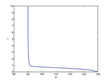
(a) $(S,I)$

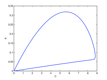
(b) $(C,A)$

Figure 1. Global stability of the disease free equilibrium (3.1) for $\mu=1/70$, $\Lambda=2$, $\beta=0.001$, $\eta_{C}=0.04$, $\eta_{A}=1.3$, $\omega=0.09$, $\rho=0.1$, $\phi=1$, $\alpha=0.33$ and $d=1$.

In Figure 2, we can observe the stability of the endemic equilibrium proved in Theorem 2 for the paremeter values $\mu=1/70$, $\Lambda=2$, $\beta=0.002$, $\eta_{C}=0.04$, $\eta_{A}=1.3$, $\omega=0.09$, $\rho=0.1$, $\phi=1$, $\alpha=0.33$ and $d=1$, which corresponds to a basic reproduction number equal to $R_{0}=1.8281$ and where the unique endemic equilibrium is given by $\Sigma_{+}=(S^{*},I^{*},C^{*},A^{*})=(76.5820,3.9959,38.3171,0.2973)$.

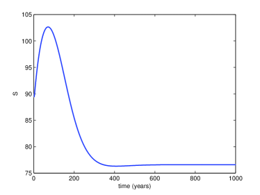
(a) $(S,I)$

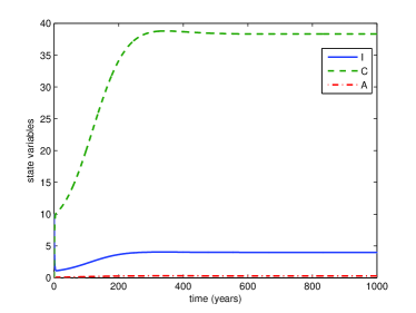
(b) $(C,A)$

Figure 2. Global stability of the endemic equilibrium of Lemma 2 for $\mu=1/70$, $\Lambda=2$, $\beta=0.002$, $\eta_{C}=0.04$, $\eta_{A}=1.3$, $\omega=0.09$, $\rho=0.1$, $\phi=1$, $\alpha=0.33$ and $d=1$.

6. Conclusion

We proposed a mathematical model for HIV/AIDS transmission with variable total population size and different transmission rates depending on the viral load of HIV infected individuals. We proved existence of a disease free equilibrium and computed the basic reproduction number $R_{0}$ using the method in [26]. Existence of an endemic equilibrium is proved for $R_{0}>1$. We also proved the global stability of the disease free equilibrium when $R_{0}<1$ and the global stability of the endemic equilibrium for $R_{0}>1$. The proofs of global stability are carried out through Lyapunov’s direct method combined with LaSalle’s invariance principle. The numerical simulations provided in Section 5 illustrate the obtained stability results.

References

• [1] U. L. Abbas, R. M. Anderson and J. W. Mellors, Potential Impact of Antiretroviral Chemoprophylaxis on HIV-1 Transmission in Resource-Limited Settings, PLoS ONE 2 (2007), e875.
• [2] R. M. Anderson, The role of mathematical models in the study of HIV transmission and the epidemiology of AIDS J. AIDS 1 (1988), 241–256.
• [3] R. M. Anderson, G. F. Medley, R. M. May and A. M. Johnson, A Preliminary Study of the Transmission Dynamics of the Human Immunodeficiency Virus (HIV), the Causative Agent of AIDS, IMA J. Math. Appl. Med. and Biol. 3 (1986), 229–263.
• [4] S. M. Blower, D. Hartel, H. Dowlatabadi, R. M. Anderson and R. M. May, Drugs, Sex and HIV: A Mathematical Model for New York City, Phil. Trans. R. Soc. Lond. B 321 (1991), 171–187.
• [5] L. Cai, X. Li, M. Ghosh and B. Guo, Stability analysis of an HIV/AIDS epidemic model with treatment, Journal of Computational and Applied Mathematics 229 (2009), 313–323.
• [6] P. W. David, G. L. Matthew, E. G. Andrew, A. C. David and M. K. John, Relation between HIV viral load and infectiousness: A model-based analysis, The Lancet 372 (2008), no. 9635, 314–320.
• [7] S. G. Deeks, S. R. Lewin and D. V. Havlir, The end of AIDS: HIV infection as a chronic disease, The Lancet, 382 (2013), no. 9903, 1525–1533.
• [8] R. Denysiuk, C. J. Silva and D. F. M. Torres, Multiobjective approach to optimal control for a tuberculosis model, Optim. Methods Softw. 30 (2015), no. 5, 893–910. arXiv:1412.0528
• [9] H. Hai-Feng, C. Rui and W. Xun-Yang, Modelling and stability of HIV/AIDS epidemic model with treatment, Applied Mathematical Modelling 40 (2016), 6550–6559.
• [10] H. W. Hethcote, The mathematics of infectious diseases, SIAM Rev. 42 (2000), 599–653.
• [11] H. W. Hethcote and J. W. Van Ark, Modeling HIV Transmission and AIDS in the United States, Lecture notes in Biomathematics, Springer-Verlag, New York, 1992.
• [12] H. Huo and L. Feng, Global stability for an HIV/AIDS epidemic model with different latent stages and treatment, Applied Mathematical Modelling 37 (2013), 1480–1489.
• [13] J. M. Hyman and E. A. Stanley, Using mathematical models to understand the AIDS epidemic, Mathematical Biosciences 90 (1988), 415–473.
• [14] V. Lakshmikantham, S. Leela and A. A. Martynyuk, Stability Analysis of Nonlinear Systems, Marcel Dekker, Inc., New York and Basel, 1989.
• [15] J. P. LaSalle, The Stability of Dynamical Systems, in: Regional Conferences Series in Applied Mathematics, SIAM, Philadelphia, 1976.
• [16] J. Li, Y. Yanga and Y. Zhoub, Global stability of an epidemic model with latent stage and vaccination Nonlinear Analysis: Real World Applications 12 (2011), 2163–2173.
• [17] Z. Mukandavire and W. Garirar, Effect of Public Health Educational Campaigns and the Role of Sex Workers on the Spread of HIV/AIDS among Heterosexuals, Theoretical Population Biology 72 (2007), 346–365.
• [18] R. Naresh, A. Tripathi and S. Omar, Modelling the spread of AIDS epidemic with vertical transmission, Applied Mathematics and Computation 178 (2006), 262–272
• [19] F. Nyabadza, Z. Mukandavire and S. D. Hove-Musekwa, Modelling the HIV/AIDS epidemic trends in South Africa: Insights from a simple mathematical model, Nonlinear Anal. Real World Appl. 12 (2011), 2091–2104.
• [20] A. Rachah and D. F. M. Torres, Mathematical modelling, simulation, and optimal control of the 2014 Ebola outbreak in West Africa, Discrete Dyn. Nat. Soc. 2015 (2015), Art. ID 842792, 9 pp. arXiv:1503.07396
• [21] H. S. Rodrigues, M. T. T. Monteiro and D. F. M. Torres, Vaccination models and optimal control strategies to dengue, Math. Biosci. 247 (2014), 1–12. arXiv:1310.4387
• [22] A. Sani, D. P. Kroese and P. K. Pollet, Stochastic Models for the Spread of HIV in a Mobile Heterosexual Population, Math Biosc 208 (2007), 98–124.
• [23] D. Sharma, Modelling and analysis of the spread of AIDS epidemic with immigration of HIV infectives, Mathematical and Computer Modelling 49 (2009), 880–892.
• [24] C. J. Silva and D. F. M. Torres, A TB-HIV/AIDS coinfection model and optimal control treatment, Discrete Contin. Dyn. Syst. 35 (2015), no. 9, 4639–4663. arXiv:1501.03322
• [25] A. Tripathi, R. Naresh and D. Sharma, Modelling the effect of screening of unaware infectives on the spread of HIV infection, Applied Mathematics and Computation 184 (2007), 1053–1068.
• [26] P. van den Driessche and J. Watmough, Reproduction numbers and subthreshold endemic equilibria for compartmental models of disease transmission, Math. Biosc. 180 (2002), 29–48.