Headphones on the wire
Statistical patterns of music listening practices

Abstract

We analyze a dataset providing the complete information on the effective plays of thousands of music listeners during several months. Our analysis confirms a number of properties previously highlighted by research based on interviews and questionnaires, but also uncover new statistical patterns, both at the individual and collective levels. In particular, we show that individuals follow common listening rhythms characterized by the same fluctuations, alternating heavy and light listening periods, and can be classified in four groups of similar sizes according to their temporal habits - “early birds”, “working hours listeners”, “evening listeners” and “night owls”. We provide a detailed radioscopy of the listeners’ interplay between repeated listening and discovery of new content. We show that different genres encourage different listening habits, from Classical or Jazz music with a more balanced listening among different songs, to Hip Hop and Dance with a more heterogeneous distribution of plays. Finally, we provide measures of how distant people are from each other in terms of common songs. In particular, we show that the number of songs $S$ a DJ should play to a random audience of size $N$ such that everyone hears at least one song he/she currently listens to, is of the form $S\sim N^{\alpha}$ where the exponent depends on the music genre and is in the range $[0.5,0.8]$. More generally, our results show that the recent access to virtually infinite catalogs of songs does not promote exploration for novelty, but that most users favor repetition of the same songs.

The reasons why human beings like listening to music, the variety of emotions music can arouse, its uses and functions in human societies: those are some long lasting questions which have been discussed by music critics and by scientists belonging to a wide range of disciplines. From the early musicology Adorno:1938 to popular music studies LeGuern:2010 through sociology of cultural practices Bourdieu:1984 , geography Carney:1998 ; Lee:2012 , music history Cohn:1972 ; Guralnick:1986 , cultural economics Cox:1995 ; Prieto-Rodriguez:2000 , educational and cognitive psychology Sloboda:1999 ; North:2000 ; Miranda:2009 ; Hallam:2011 , physiology and neurosciences Levitin:2006 ; Salimpoor:2009 , an eclectic scientific litterature has illuminated many different facets of music listening. At a collective level, it has been demonstrated several times that statistical relations between inherited social characteristics of individuals and their musical preferences exist Bourdieu:1984 ; Prior:2011 ; Bryson:1996 ; VanEijck:2001 . At the individual level, studies relying on questionnaires, interviews or experiments conducted in controled environments have documented both the functions attributed to listening and the emotions aroused, in various situations of daily life and in different contexts Juslin:2004 ; Sloboda:1999 ; Hallam:2011 ; Salimpoor:2009 . The influence of the device on the listening practice Krause:2013 , the effects of listening on a number of daily activities – e.g. performance at work Lesiuk:2005 , driving Dibben:2007 , coping and regulating emotions Miranda:2009 ; Saarikallio:2010 – or the rewarding aspects of music-evoked sadness Taruffi:2014 are other examples of listening-related research. Classifications of listeners have been proposed, with some authors concluding about the existence of a direct relation between musical preferences and cognitive styles Greenberg:2015 , other stressing the uses of music and their self-declared importance as relevant classifiers TerBogt:2011 ; Schafer:2016 . Statistical physicists also contributed by highlighting structural properties of artists and genres communities that emerge from the analysis of personal libraries of audio files Lambiotte:2005 .

However, relatively little is known about how precisely we listen to recorded music on a daily basis. By how we refer here to some kind of detailed, quantified radioscopy of our contemporary listening practices of recorded music, an important aspect of the relation we entertain with music.

Until recently, any empirical research willing to answer to questions pertaining to daily listening practices had to rely on surveys and interviews. The technological and societal evolutions have sustained the development of new mobile devices, online tools and listening possibilities, as well as new actors in the music industry. Music-on-demand services have quickly gained in popularity over the last few years, and for example, according to a recent report of the French national syndicate of phonographic publishing SNEP:2016 , more than three million of French residents (approx. 4% of the total population) were subscribing to an on-demand streaming music platform in 2016, and roughly $1/3$ of the total french population regularly stream audio content. The data recorded by streaming platforms offer great possibilities to analyze and hopefully better understand individual and collective listening practices.

Whenever an individual plays a song through such a service, with a web browser or dedicated application, online or offline, all known information associated with the stream are logged in the company’s database. For example, when Amélie plays The Roots’ Kool On on her mobile phone, a new entry is added to the database, informing that at 8:23 am on 2/10/2015 she played the song (Kool On) by The Roots, from the album Undun. Incidentally, we also know the genres tags associated to the song, the stream’s duration (and consequently if she listened to the song entirely or not), the information declared during registration, including her age and city of residence, and possibly some additional contextual information (e.g. if the song was part of one of Amélie’s playlists, if she was online or offline when listening to the song, possibly the city where Amélie was located when listening, etc.). Such a record of information is added to the database for each single play of the millions of registered users of the service. Once anonymized, users’ listening history data can be processed and analyzed, and those digital traces passively produced while listening consequently constitute an unprecedented empirical source to study quantitatively contemporary listening practices.

In the following we analyze the listening history data of one of the major streaming platforms. The data correspond to the entire listening history of about five thousands users during one hundred days (see Material for details). We note that for some of these people the music streamed may represent only a limited subset of all the recorded music they listened to during that period, and their data might not be representative of their entire listening practice Krause:2013 . In order to control this bias we selected a set of anonymous users among those who displayed a frequent use of the service (see Appendix). For these listeners we can reasonably assume that the streaming platform, if not exclusive, constitutes a daily source of music.

Results

Rhythms

We start by quantifying the relation that individuals have with music listening as a daily activity, and the rhythms and typical hours at which they perform this activity. For all individuals, we compute the total time they spent listening during the 100 days period under study. Fig. 1a represents the cumulative distribution of the average daily listening time $\bar{t}$ computed over all individuals and all days. This quantity varies theoretically from $0$ to $1440$ (number of minutes in a day) and the empirical measure reveals a range from $4$ to $1200$ minutes per day, a median value of approximately $80$ minutes, and about $75\%$ of individuals listening more that one hour per day (and $25\%$ listening more than 2 hours per day). In order to understand how listeners behave over periods of several months, we extract the distribution of the daily listening times $t_{i}$ for all individuals (the index $i$ refers to the individual) and for the whole period, splitting listeners into three groups according to their total listening time (“light”, “medium” and “heavy” listeners). We compute for each individual its average $\bar{t_{i}}$ over all days and we show on Fig. 1b the normalized $(t_{i}/\bar{t_{i}})$ distributions for the three groups. These normalized distributions collapse onto a single curve, indicating that whatever how much music they listen to, individuals display a common behavior characterized by the same fluctuations in listening times, alternating days with relatively few music listened and days of heavy listening. These distribution are peaked and can be fitted by an exponential function, suggesting a Poisson nature of the listening behavior, in contrast with previous results on daily human behavior Barabasi:2005 .

We then wonder at what time of the day people listen to music. We introduce $u(h)$ which counts the number of individuals listening to music at time $h$. In order to highlight the collective rhythm we plot the normalized values $\int_{h}^{h+1}u(h)/\int_{0}^{23}u(h)$, where $\int_{0}^{23}u(h)$ is the total number of unique individuals that listened to music during the day (see Supplementary Figure 1). Like other daily activities which have been heavily studied from individual traces Lenormand:2014 ; Lenormand:2015 the aggregated curves of activity display two characteristic patterns, one for weekdays and another for weekends. However not everyone listens to music at the same hours, and for each listener $i$ we calculate his/her proportion $p_{i}^{h}$ of plays that occurred between $h$ and $h+1$, averaged over the 100 days period. We then construct the 24-values vector $(p_{i}^{0},\dots,p_{i}^{23})$ and using these time profiles we cluster the listeners, and find four typical groups whose average profiles are shown in Fig. 1c (see the Appendix for details on the clustering). These time profiles are very specific: in one group individuals listen to music mostly in the morning (“Early birds”); in another we observe two listening peaks, one in the morning and the other in the afternoon (“Working hours listeners”); there are also individuals listening to music mostly at the end of the day (“Evening listeners”); and finally those whose listening peak is late in the evening and during the night (“Night owls”).

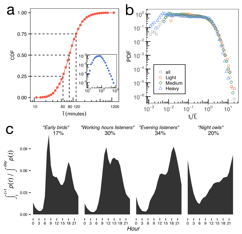
Figure 1: Music listening rhythms. (A) Cumulative distribution of the average daily listening time $\bar{t}$ (in minutes) computed over all listeners and all day. The y-value of each point gives the fraction of users that listened at most $\bar{t}$ minutes of music each day on average, during the 100 days period under study – inset: corresponding probability distribution. (B) The normalized distributions of daily listening times $(t_{i}/\bar{t_{i}})$ for three different groups of listeners: heavy listeners (more than 2 hours per day on average, blue triangles), medium (between 1 and 2 hours, green diamonds), and light (less than 1 hour per day, orange squares).(C) Average profiles of different groups of listeners obtained by clustering on their listening temporal habits.

Difference and repetition

We now investigate how individuals are distributed along various dimensions of music listening. We denote by $P_{i}$, $S_{i}$, and $A_{i}$ the total numbers of plays, unique songs and unique artists listened by individual $i$ during the 100 days period, respectively. We show on Fig. 2a the distribution $p(P/\bar{P})$, $p(S/\bar{S})$ and $p(A/\bar{A})$ of the normalized variables (where the average values are computed over all individuals and the whole 100 days period). These distributions collapse on a curve that can be fitted by a log-normal distribution of parameters $\mu\approx 3.9$ and $\sigma\approx 1.1$. It is here another occurrence of the lognormal distribution in social dynamics, although its origin here is not clear and would deserve further investigation. Also, while we can understand a priori that $P$ and $S$ display the same behavior, it is more surprising that the distribution of the number of unique artists listened also collapses on the same curve.

In order to understand how individuals distribute their plays among the songs they listen to, we compute the aggregated distributions $p(P_{i}(\alpha))$ which contain the numbers of plays per song $\alpha$ for each listener $i$ (we then have $\sum_{\alpha}P_{i}(\alpha)=P_{i}$) for the three groups defined above – heavy, medium and light listeners, according to their total number of plays. We represent in Fig. 2b these distributions $p(P_{i}(\alpha)/\overline{P_{i}(\alpha)})$ (with $\overline{P_{i}(\alpha)}=P_{i}/S_{i}$) which also collapse on a curve whose tail can be fitted by a power law with an exponent $\approx 3.0$ (the distributions $p(P_{i}(\alpha))$ are shown in the inset). The fluctuations around the average value $P/S$ are therefore the same whatever the group: no matter how much music people listen to, they distribute similarly their attention on the different songs listened. Patterns of Fig. 2a and b might result from a simple relation between $P$, $S$ and $A$ common to all listeners and that would allow to make predictions for any of these variables knowing the value of another. As shown on Supplementary Figure 4, there are however no clear relations among these variables and we observe large fluctuations from one person to another.

We now focus on the quantity $S_{i}/P_{i}$ which can be seen as the exploration rate of individual $i$ among the catalog. By definition this ratio varies between 0 – the extreme case of an individual that would listen to one and only song again and again – and 1 – a pure explorer that would never listen a song twice. The binned scatterplot of Fig. 2c shows that there is no clear relation betweeen the weight of exploration $S/P$ and the total time spent listening to music (characterized by $P$). We also see that the average value of $S/P$ is around $1/3$, indicating that the average number of plays per song is $\approx 3$. We observe a trend (despite large fluctuations) between the average rate $\overline{S_{i}/P_{i}}$ and the listeners’ age (shown in Fig. 2d; errors bars correspond to one standard deviation), indicating a decrease of repetition and an increase of exploration with age (see also Lamere:2014a ).

Streaming audio is a different experience than listening to the radio or browsing in a personnal collection of records or audio files. Several modes are offered to users: they can search and play songs one after another, listen to an entire album or listen to a playlist previously compiled by themselves, someone else or automatically generated (the latter gaining in importance thanks to increasingly sophisticated recommendation systems Bonnin:2014 ). Vinyle records favor a sequential listening from the first to the last track, CDs allowed direct access to any song of the record but still contain albums which are “meant to” be played entirely. Streaming platforms offer listeners an immediate access to any song. The possibility to pick songs among a practically infinite catalog suggests the naive assumption that we should observe a high versatility in plays, and listening sessions mixing album-centered habits with handmade sequences of songs (in playlists or not). In order to check this hypothesis we first compute for each listener the percentage of albums listened entirely (while not necessarily in sequential order), and plot the distribution of this percentage among the population of listeners on Supplementary Figure 5. More than $50\%$ of users played in their entirety less than $5\%$ of the albums. We then compute the distribution of the number of songs played per album, and compare it to the distribution of the number of songs per album. If listeners had album-centered practices, then both distributions should match. The results shown on Fig. 2e tell a different story. The distribution of the number of songs per album in the catalog (blue curve) has several small peaks around typical values that correspond to different types of records: 1 (singles), 10–12 (the typical number of songs on albums), and then 20/30/40 (likely corresponding to double/triple albums and compilations/anthologies). In contrast we observe a very different distribution (red curve) when we consider the number of songs played per album, that displays a regular decay with a smaller peak around 10, corresponding to the remainder of album-centered listening practices.

Figure 2: Dimensions of contemporary listening practices. (A) Histogram of the total numbers of plays ($P$), songs ($S$) and artists ($A$) listened among users during the $100$ days period. (B) Normalized distributions of plays per song $P/\bar{P}$ for three groups of listeners (light, medium and heavy – according to their total number of plays). Inset: distribution $p(P_{i}(\alpha))$ for the three groups of listeners. (C) Binned scatterplot of the listeners’ exploratory ratio $S/P$ vs. their total number of plays $P$. (D) Exploratory ratio $S/P$ vs. listeners’age. For each age, the error bars correspond to a standard deviation. (E) Histograms of the number of songs per album in the music catalog available to listeners (blue curve) and of the number of songs played per album listened (red curve).

Music genres and listening habits

Each song is indexed with one or several genre tags. While there are hundreds of unique tags in such songs databases, most of them are associated to a very small proportion of songs only, and concern an even smaller proportion of plays. The distribution of the listeners’ plays per genre shows us first that over a period of several months, most individuals listen to songs of very different genres (see the histogram of the number of genres listened at least once on Supplementary Figure 8). This first impression of broad eclecticism is challenged by a closer look at the individuals’ distributions of plays among genres. For each individual $i$ we compute the Gini normalized coefficient (see Supplementary Methods in Appendix) of his/her distribution $p(P_{g}(i))$ of plays in each music genre $g$, and plot on Supplementary Figure 9A the distribution of this Gini coefficient among listeners. We first observe that there are no listeners displaying small Gini values. On the contrary, most individuals have large Gini values, indicating that even eclectic individuals who listen to many different genres tend to strongly favor a subset of them. From the value of the Gini coefficient we extract a typical number of dominant genres among the listener’s plays (see Supplementary Methods in Appendix). It appears that most individuals have 2 or 3 genres that they clearly favor (cf. Supplementary Figure 9B and C). This observation naturally leads us to determine the couples of genres which often go together. We then determine for each listener his/her two most listened genres, and estimate the probability $P(g_{2}|g_{1})$ to have $g_{2}$ as second favorite genre when $g_{1}$ is the favorite one. These probabilities are represented on Supplementary Figure 10. Beyond the leading role of Pop music on streaming platforms, we recognize classic proximities, such as Metal-Rock, the Hip Hop family or the Classical-Jazz tandem. We also observed that the temporal patterns of the music genres do not strongly differ from each other (see Supplementary Figure 11) Jagger:1969 . Similarly, we could not distinguish groups of artists that are preferentially listen to at certain hours Sinatra:1955 .

We now focus on 9 broad genres (Classical music, Jazz, Rock, Metal/Hard Rock, Reggae, Electro, Pop, Hip Hop, and Dance) to see if this classic, “record store alleys” classification allows to discern various listening habits. Considering how recorded music is produced and distributed, some music genres favor the emergence of “hits” and are more “inegalitarian” than others when it comes to the repartition of the crowd’s attention towards songs (see Supplementary Figure 12). The heterogeneity of the number of plays in each genre is represented by a “violin plot” shown in Fig. 3. Each genre is represented by a violin, which gives vertically and symetrically the smoothed distribution (kernel density estimation) of the listeners’ Gini coefficient for songs in that genre. The Gini coefficient of a given individual for a given genre encodes the inequality of his/her distribution of plays among the songs of this particular genre. The violins are shown from left to right according to the average value of the individuals’ Gini coefficients. These violins show that the Gini coefficient is usually distributed over the whole range $[0,1]$, indicating that for most genres there is a strong heterogeneity of listening practices. We however observe that individuals, when they listen to the most popular genres (Pop, Hip Hop or Dance), are more homogeneous and seem more focused on a subset of songs. In contrast, in other genres we observe a greater variety of listening practices (for example for Jazz or Classical). We then group listeners according to their favorite genre: Rock, Rap, Jazz, etc. We calculate the average age of the people in each group, along with the average exploration rates $S/P$ inside and outside the favorite genre (shown on the Supplementary Figure 13). We note that in all groups the exploration rate is larger outside the favorite genre than inside, an indication that for most individuals what contributes to make a genre their favorite is the repetitive listening of a small number songs of that genre. We also note substantial differences in terms of the average age of listeners in the different groups, an expected observation in agreement with previous work LeBlanc:1999 ; Prieto-Rodriguez:2000 ; Lamere:2014a .

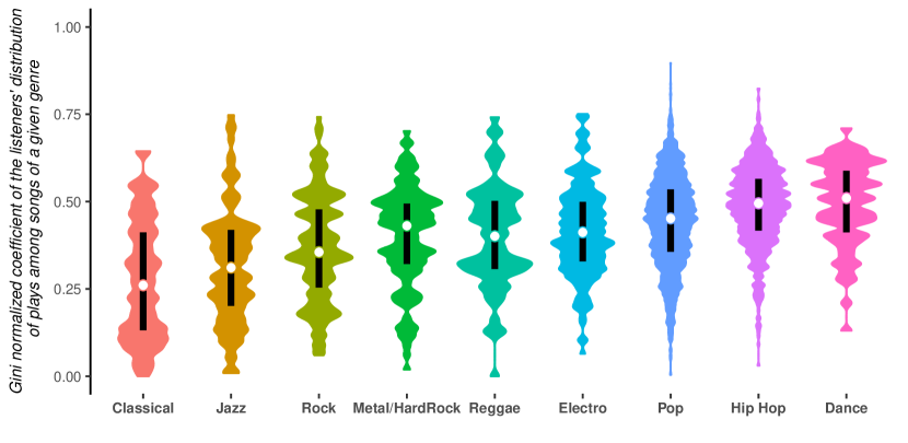
Figure 3: Inequality of music genres. Each violin is a vertical and symetric representation of the smoothed distribution (kernel density estimation) of its listeners’ Gini coefficient of plays per song, for each genre. Each violin shows to what extent individuals have an heterogeneous attention towards the songs they listen to, when they listen to that genre.

Playing music at a party

Finally, we provide measures about the “distance” between individuals in terms of the music they listen to. The size of the online music library is practically infinite which implies that individuals’ plays would have a very small overlap if random. Musical choices however depend on many things, are strongly influenced by social factors Bourdieu:1984 and we could expect a larger value of the overlap than the one obtained by chance. We first estimate from the dataset the probability that two randomly selected individuals share a given number of songs. Fig. 4a shows the probabilities $p=Prob(s\geq S,\delta t)$ that they shared at least $S$ songs during a period $\delta t$ varying between one hour and one month. This probability obviously increases as one considers longer time periods, and the probability $p(S\geq 1,\delta t=30\;days)$ that two people have listened at least one common song in 30 consecutive days is large $p\geq 0.7$ ($p\geq 0.9$ for a 100 days period). The four curves on Fig. 4a are very similar and display a cut-off value of $\approx 10-15$ songs.

A related problem is to determine the minimum number of songs that a DJ should play to an audience so that everyone hears at least one song that he/she recently listened to. This problem is well-known by non-professional DJs who have to deal with people harassing them to play specific songs at parties. This minimum number of songs $S$ obviously depends of the size $N$ of the audience, and we call the function that relates $S$ to $N$ the DJ function. In order to evaluate empirically this function, we randomly sample different sets of listeners of increasing size $N$, and for each set we determine the smallest number of songs $S$ that allow to satisfy them all (in other words, $S$ is the size of the minimum 1-mode vertex cover in the bipartite subgraph connecting the individuals sampled and the songs they listened). When plotting this number $S$ vs. $N$, we observe a behavior of the form $S\sim\sqrt{N}$, as shown by the black curve on Fig. 4b. We repeat the same calculation by focusing on specific music genres to cover the case of “specialized” DJs. We select songs (and their listeners) of a given genre only, allowing us to evaluate a DJ function per genre. Each of them has the same general form $S\sim N^{\alpha}$, with $0.64\leq\alpha\leq 0.8$ ($R^{2}>0.99$). These exponents give a lower bound to the size of the setlist that one has to play if she/he wants to “satisfy” everybody in a random crowd full of strangers. In particular, if the venue is big and the audience large ($\geq~{}10^{4}$ individuals), the required number of songs will be too large to be played during a single event, making the challenge impossible whatever the DJ. In reality, the crowd attending to a gig is not random and gather individuals with similar taste. We then reproduce the same experiment but this time by considering specialized audiences, composed of people whose favorite genre is the one played by the DJ. As expected we obtain smaller exponents, with $0.47\leq\alpha\leq 0.8$ ($R^{2}>0.99$), showing that specialized audiences are easier to “satisfy”.

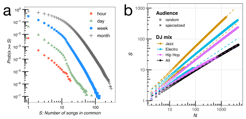
Figure 4: Organizing a party. (A) Estimated probabilities that two randomly chosen individuals listened at least to $S$ common songs, for different periods of time. (B) DJs’ functions capturing the relation between the size $N$ of an audience and the minimal number of songs $S$ one should play so that everybody in the room hears at least one song that he/she recently listened to. Colours correspond to DJs playing specific music genres, while shape of points correspond to random or specialized audiences.

Discussion

Streaming platforms contribute to increase possibilities of access to recorded music, and might possibly change the listening habits of their users. These can experience legal and unlimited access to a gigantic catalogue containing more years of unique music than what one could listen to in an entire life. Our results challenge a number of naïve assumptions about the contemporary forms of an old and widespread cultural practice. Considering the available catalog, one could think that it would encourage listeners to continuously search for novelty, and browse in many genres, artists and albums. Our results on the weight of repetition and the small number of dominant genres per listener indicate that it is currently not the case. This observation takes place in the context of discussions about the psychological function of repetition when listening to music. These considerations are however beyond the scope of this article, and we refer the readers to more specific work relying either on detailed interviews with listeners Sloboda:1999 ; Kamalzadeh:2016 , self-reports TerBogt:2011 or neuroimaging Levitin:2006 . We remind however that “talk is cheap” Jerolmack:2014 , and our observations that (i) heavy and light listening days identically alternate whatever the perceived importance of music in the listeners’ daily lives, and (ii) that the weight of repetition is independent of the amount of music listened, challenge previous results based on questionnaires and interviews.

It would be wise nonetheless not to generalize too hastily our results to music listening practices in general, whatever the listening device. The availability of pre-existing playlists and the automated generation of playlists fitted to the users’ taste might encourage a less involved listening process, resulting in distinct statistical properties between “active” and “passive” listeners. For example, the authors of Greasley:2011 concluded that those who declare listening more music are also more involved in the choice of the music they listen to. The data we analyzed include no contextual information that let us know if the songs listened were voluntarily played after a proper search, or if they were recommended and queued by the service itself. We should also mention that there is so far a limited proportion of individuals who use streaming platforms as their main source of recorded music, but this proportion is constantly increasing SNEP:2016 . We have restricted our analysis to listeners whose activity suggests that they favor streaming. But considering that these may not representative of the entire population (in terms of social and demographic criteria), our results need to be confirmed with richer datasets providing more contextual information.

The collection of individual data by companies raises privacy issues and legitimate concerns about surveillance. For obvious reasons these companies are reluctant to share the raw data they collect, even after proper anonymisation. This policy partly explains why very few results obtained from such data have been published so far in the scientific literature. Questions similar to those we addressed are nonetheless studied internally in a product-oriented research (see for example Spotify Insights SpotifyInsights or Music Machinery,, collections of blog posts discussing data-driven analysis of listening practices, e.g Lamere:2014 ). However, “digital footprints” alone do not give researchers clues about the individuals’ intentions explaining their behavior and choices. More generally, these traces poorly inform about the context of use, suffer several uncontrolled bias, and might lead to misinterpretating the results Lewis:2015 (e.g. was the user really listening – or even in the room – when the song was played?). Consequently any “blind” analysis of logs alone is doomed to be limited in scope, and in some cases may lead to wrong conclusions (e.g. see Gallotti:2016 for a discussion of the case of individual human trajectories reconstructed from unconventional data sources). While an increasing part of daily human activities produce electronic traces, designing information collection protocols which articulate the strengths of both traditions (detailed surveys and interviews in one hand and digital footprints in the other) is a contemporary challenge faced by social research.

Material and Methods

Dataset

The dataset analyzed contains the raw streaming data of 10,000 anonymous and registered users of a major streaming platform. They inform us on their entire listening history during the 6-months period spanning from June 1st 2013 till December 1st 2013. These users were randomly selected among all the registered French users of the service. We know nothing about how important is the streaming service for these users, who might also heavily rely on other music sources and devices (their own personal library of records or audio files, the radio, etc.), and might have distinct practices depending on the source and device Sloboda:1999 ; Krause:2013 ; Kamalzadeh:2016 . In order to mitigate this bias, we chose to focus on users who made a frequent use of their account. We selected a set of 4,615 anonymised French users who actively listened to music (at least every other day in average) during a 100 days period, from 2013/8/15 to 2013/11/23. For these individuals we can reasonably make the hypothesis that streaming, if not their unique, was one of their main music source during this period (see the Appendix for details on the cleaning and filtering of the data).

Normalized Gini coefficient and extraction of the number of dominant terms

We assume that we have $K$ classes and in each class, we have a random number $X_{i}$. The Gini coefficient can then be computed as follows

$$G_{K}(X)=\frac{1}{2K^{2}\overline{X}}\sum_{p,q}|X_{p}-X_{q}|$$ (1)

This coefficient is a priori in the interval $[0,1]$ but we will see that for finite $K$ the maximum value is actually different from 1 and depends on $K$.

Case $K$ and $D=1$

We denote by $D$ the number of dominant terms. If $D=1$ we have only one dominant term that we call $X_{1}=a$ and all the other terms are much smaller than $a$ and for simplicity – without any loss of generality – we take them $X_{i\neq 1}=1$. The Gini coefficient is then

$$G_{K}(a) =\frac{1}{K^{2}}\frac{(a-1)(K-1)}{\frac{a+K-1}{K}}$$

$$=\frac{K-1}{K}\frac{a-1}{a-1+K}$$

In the limit $a\gg K$ where the heterogeneity is maximal and the Gini coefficient maximum, we then obtain

$$G^{*}_{K}=\frac{K-1}{K}$$ (2)

We see on this formula that $G^{*}$ can actually be much smaller than 1 if $K$ is not too large. In the case of a small $K$ we thus have to compute the normalized Gini coefficient $G/G^{*}_{K}$ which is in the interval $[0,1]$ and reaches $1$ for the most heterogeneous distribution.

General $K$ and $D$ case

We assume here that we have $D$ dominant terms and for simplicity we assume that $X_{1}=X_{2}=\dots=X_{D}=a$ and $X_{i>D}=1$. We then have

$$\overline{X}=\frac{Da+(K-D)}{K}$$ (3)

We also obtain

$$\sum_{p,q}|X_{p}-X_{q}|=2D(K-D)(a-1)$$ (4)

and the Gini coefficient is then

$$G_{K,D}(X) =\frac{1}{2K^{2}}\frac{2D(K-D)(a-1)}{\frac{Da+(K-D)}{K}}$$ (5)

$$=\frac{K-D}{K}\frac{D(a-1)}{Da+K-D}$$ (6)

In the limit where $a\gg 1$ we then obtain the maximum value

$$G^{*}_{K,D}=\frac{K-D}{K}$$ (7)

Extracting the number of dominant terms

For a given observation of the Gini coefficient for $\{X\}$, we can ask what is the equivalent configuration with $D_{eff}$ dominant terms ? In other words, if we measure G, this value is bounded

$$\frac{K-D}{K}<G<\frac{K-D+1}{K}$$ (8)

where the number of effective dominant terms is given by

$$D_{\text{eff}}=E[K(1-G)]$$ (9)

where $E[x]$ denotes the nearest (lower) integer of $x$.

Data availability

The raw data that support the findings of this study were provided by a third-party company. Restrictions apply to the availability of these data, which were used under license for the current study, and are not publicly available. Derived, aggregated data supporting the findings presented in this article are however available from the corresponding author upon request.

Appendix

Data pre-processing

After signing a non-disclosure aggrement (NDA) with a major music-on-demand company, we were given access to a dataset containing the raw streaming data of 10,000 anonymous users of the service. These anonymous users were randomly selected among all the registered French users of the service. The streaming data correspond to their entire listening history during the 6-months period spanning from June 1st 2013 till December 1st 2013. The users were sampled uniformly among all their French users (no bias regarding suscription plan, listening activity, sex, age, geographical location or years of use). Consequently the listening data are those of users with different types of usage of the service. In particular, some of them are paying suscribers, while some other aren’t (”free” suscribing users). The latter have to listen advertisement between songs, cannot listen offline, the audio quality is lower, and for some of them the total listening time is bounded. We note that these combined aspects can obviously influence the listening activity, probably decreasing the time spent using the service each day.

Our goal was to focus on individuals who use the music-on-demand streaming platform as one of their main music sources (if not the main one). Consequently we applied a number of filters to select relevant users and eliminate those whose streaming data may not be representative of their listening habits in general, whatever the source and device. The data include a few information on the users’ profiles (self-declared age, sex and city of residence), but we do not know if the user is a paying suscriber or not, and could not get this information from the company. It prevented us to simply filter them.

From the data we inspected the number of unique users per day and realized that it displays large fluctuations. Not all users were active during the entire 6-month period (some appearing only after a given date, some disappearing). To circumvent this we focused on a 100 days period (from 15/08/2013 to 22/11/2013) during which the number of unique listeners per day remained stable. We then selected users who displayed regularity in their use of the service during this 100 days period and used the service one every two days in average. Hence the filter is not on the total activity (listening time) of the users but on their frequency of use. We ended with 4,615 anonymous users.

Supplementary Methods

Clustering listeners according to their daily streaming rhythms

For each user $i$ we construct a 24-values vector $(p_{i}^{0},\dots,p_{i}^{23})$, where $p_{i}^{h}$ is the proportion of the user’s plays that took place between hour $h$ and hour $h+1$, during the 100 days period. We clusters these vectors with the k-means method. A usual question when clustering $n$ individuals into $k$ clusters (with $k$ fixed a priori) is to determine an appropriate value of $k$. A small $k$ value will result is a very simple picture but which may poorly capture the fluctuations in the data, while $k\sim n$ will capture the variance almost perfectly but will be useless. To determine a reasonnable range of values for $k$ we plotted on Supplementary Figure 2 the averaged percentage of variance captured by $k$ clusters resulting from the application of k-means to the $n$ listeners. From this curve we use the ’elbow method’ to determine the range of reasonnable values for $k$. It appears that $4=<k<=12$ are candidates, and we looked at the average time profiles resulting from the clustering with each value of $k$. From $k>=5$ we observed less distinct average profiles, which is why we kept $k=4$ for the figure discussed in the main text.

Characterizing individual distributions of plays

Supplementary Figure 3 gives the distribution of the listeners’ Gini coefficient resuming the heterogeneity of their distribution of plays among songs (see the Methods section of the main text). Listeners who have a small Gini value (typically $<0.3$) are those whose distribution is almost flat, indicating that they listened their songs approximately the same number of times. For such listeners the average value $P/S$ (with $P$ the total number of plays and $S$ the total number of unique songs listened) gives a clear picture of their listening practice and of their repetition/discovery behavior. But for a large proportion of individuals the Gini coefficient is large ($>0.5$), revealing that these users have concentrated their plays on a limited number of songs.

S vs. P.

On Supplementary Figure 4A we plot for each user $i$ her/his number $S_{i}$ of distinct songs listened versus her/his total number of plays $P_{i}$ (here limited to the individuals with $P<5000$ – which captures 95% of listeners). Each single point represents an individual, and we see points distributed all across the triangle (by construction we have $S<=P$), which indicates a wide variety of profiles in terms of repetition/exploration. Some listen to a relatively small number of songs and listen to them a lot (small $S$ and large $P$ case), while to the opposite some other listen to many different songs and listen each of them a few number of times (the points near the dashed line $S=P$). Another way to capture the tendency of individuals to concentrate their plays on a limited fraction of the songs listened is to calculate the relative dispersion $\sigma_{i}/\mu_{i}$ of their distribution of plays per song $(P_{i})$. The histogram of $\sigma_{i}/\mu_{i}$ on Supplementary Figure 3B shows that there exists several types of listeners. Individuals with $\sigma/\mu\ll 1$ have a distribution of plays per song peaked around the mean, and the average number of plays per song $\bar{p}_{i}$ is hence an informative value. To the contrary for individuals with $\sigma/\mu\gg 1$, the average number of plays per song $P_{i}/S_{i}$ would not be representative of their listening practice.

Selection and aggregation of music genres

Each song of a music-on-demand service is tagged with one or several tags (in the following we name them basic genres tags and the histogram of the number of tags per song is displayed on Supplementary Figure 7). The weight of these basic genres – measured through their total number of songs in the streams – is very different from one genre to another. Furthermore, the analysis of the network of basic genre tags reveal different types of tags, and some hierarchical relations between them (some entirely include/contain others). We build the weighted and directed network $S_{ij}$ of genre tags. It is the 1-mode projection of the bipartite network linking songs and genres tags. In this network the nodes represent the basic genres, and $S_{i\rightarrow j}=k$ means that there are $k$ songs tagged with genre $i$ which are also tagged with genre $j$ (the network is directed and in most cases $S_{i\rightarrow j}\neq S_{j\rightarrow i}$). Some basic genre tags correspond to very broad, higher-order categories (e.g. ’Pop’, ’Rock’ ’Alternative’, ’Dance’) and serve as coarse-grained classifiers. The analysis of this network reveals that it has a hierarchical structure and that some of these genres tags entirely “contain” smaller, more informative tags. For example all “Blues” songs are also tagged as being “Rock” songs, and all “Metal/Hard-Rock” songs are also tagged as “Rock”. On the contrary, there are some “Rock” songs that are tagged only as “Rock”. The purpose of the filtering we performed and detail below was then to keep the most informative/precise tag(s) for each song, whenever it is possible and relevant.

To perform our genre analysis, we start with the same dataset $D$ used in subsections 1 (Rhythms), 2 (Difference and repetition) and 4 (Playing music at a party) of the results section in the main text. This dataset contains the entire streams history of the 4,615 users during 100 days. We first merge this dataset with the songs database provided by the music-on-demand company, which contains the genre tags associated to each song of the catalog. It results in a dataset $D^{\prime}$ giving us the complete streams associated to each of the basic genre tags. We filter this dataset of $\approx 2*10^{7}$ entries by applying the following rules:

• we remove the purely “geographical” tags (World, France, Europe, North America, Central America/Caribean, South America, Brazil, Africa, Maghreb, Middle East, Australia/Pacific) which give limited information on the music genre itself;

• we filter out the basic genre tags which account for less than $0.01\%$ (nb: arbitrary parameter choice) of the songs listened – including ”Bollywood”, ”Finnish folk”, ”Medieval”, ”Chaabi”, ”Comptines/Chansons”, ”Mento/Calypso”, ”K-Pop”, ”Celtic music, ”Bachata”, ”Classical turkish music”, ”Axé/Forró”, ”Regional méxicain”, ”Instrumental Hip Hop, ”Mariachi”, ”Argentinian folklore”, ”German rap”, ”Banda”, ”Nederlandstalige volksmuziek”, ”Brasilian rock”, ”South-African House”,”Teen thaï”, etc. –, in order to reduce the number of genres compared and focus on the most listened ones; after this step we have discarded $\approx 40$% of the basic genre tags.

• we keep all the streams of songs which are tagged with one basic genre tag only ($\approx 3\times 10^{5}$ songs); the basic genres tags that are used as single tags are the following: Hip Hop, Dance, Pop, R&B/Soul/Funk, Reggae, Electro, Rock, Alternative, International pop, Jazz, Classical, Variété, Country, Brasil, Music for kids, French chanson, Movies/Video games, Tropical, Latin rock.

• for the remaining streams of songs tagged with two or more basic genres tags ($\approx 2.5\times 10^{5}$ songs), we inspect the statistic of the pairs of basic genres tags among songs. For each pair of basic genres $(g,g^{\prime})$, if it appears that $g$ entirely contains $g^{\prime}$ (i.e. all songs tagged as $g^{\prime}$ are also tagged as $g$), then we remove $g$ from the corresponding streams (i.e. streams which were previously associated to these two basic genres will now be associated only with genre $g^{\prime}$). For example, let’s say we wish to calculate aggregated statistics for “Rock”, “Blues” and “Metal” streams. Since all songs tagged as “Blues” (resp. “Metal”) are also tagged as “Rock”, to come up with more relevant statistics for the three genres we consider that it is more significant to discard streams associated to “Blues” and “Metal” songs when computing reference statistics for “Rock” streams (and keep in the “Rock” category limited to the songs tagged solely as “Rock” ). We end up in removing basic genre tags such as Pop, Rock, Electro, Hip Hop, Jazz, Classical, etc. among the tags that qualify songs with 2 or more tags, because they are systematically associated with more informative tags (e.g. indie rock, Metal/hard-rock, Blues, Techno/House, rock’n roll/rockabilly, Funk, chill out/trip-hop, instrumental jazz, instrumental hip-hop, opera, etc.).

We end up with more than $7\times 10^{6}$ streams. The statistics of the number of basic genre tags per song in the remaining filtered streams are given in Table 1. More than 90% of the songs are tagged with 1 genre only, and almost all songs (98%) are tagged with 1 or 2 genres, limiting the risks of confusion in the analysis of listening patterns associated to various genres.

#genres	#songs	weight
1	439582	9.002220e-01
2	38348	7.853304e-02
3	9384	1.921754e-02
4	970	1.986467e-03
5	20	4.095809e-05

Table S1: Number and proportion of songs having a given number $k$ of genre tags, after filtering and removing higher-order genre tags.

Supplementary Figures

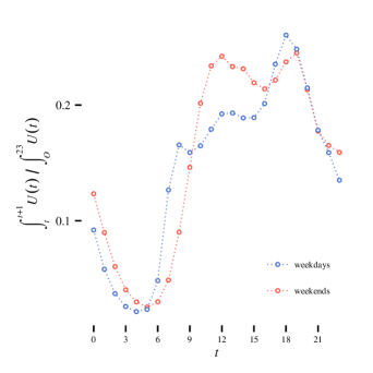
Supplementary Figure 1: Hourly evolution of the proportion of active listeners, during an average weekday and an average weekend day.During weekdays the number of individuals listening to music increases over the day to reach a maximum around 7-8 p.m. We notice two small peaks, one in the morning aroung 8 a.m. and the other one at lunchtime around 1 p.m. Most of the plays occur during the afternoon and evening. During weekends the collective rhythm is different with two peaks, one around 12 p.m. and the other in the early evening, around 7-8 p.m. (error bars are small indicating a high regularity of temporal listening habits

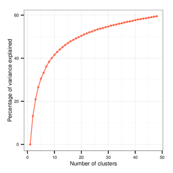
Supplementary Figure 2: Percentage of variance explained when clustering listeners in $k$ groups according to their listening time profile average over 100 days.

(a)	(b)

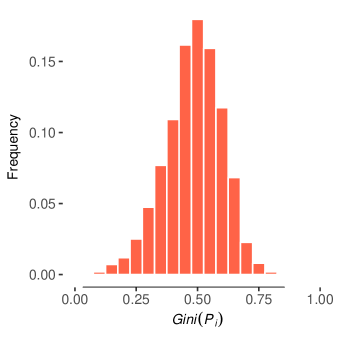
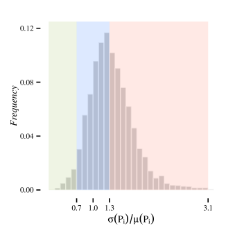
Supplementary Figure 3: (a) Histogram of the individuals’ Gini normalized coefficient resuming their distribution of plays among the songs they listened (b) Histogram of the users’ relative dispersion of plays. For each user $i$, $\mu_{i}$ is the mean value of his/her distribution of plays per song, while $\sigma_{i}$ is the standard deviation of this distribution.

(a)	(b)	(c)

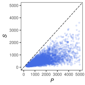
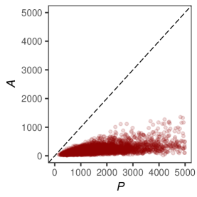
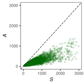
Supplementary Figure 4: On these scatterplots each dot represents a listener (a) Number of unique songs listened $S$ vs. total number of plays $P$ (b) Number of unique artists listened $A$ vs. total number of plays $P$ (c) $A$ vs $S$. The data appears clouded, we see a lot of fluctuations and no clear relation linking $P$, $S$ and $A$ that would allow to make predictions.

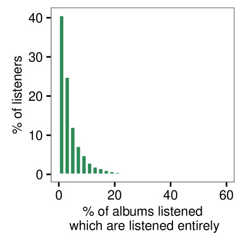
Supplementary Figure 5: Proportion of albums listened entirely (but not necessarily in just one time and sequential order). More than 50% of the users listened entirely less than 5% of all the albums in which they grabbed songs, underlining that album-oriented listening sessions are clearly not the standard practice on streaming platforms.

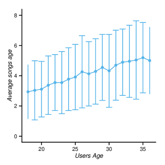
Supplementary Figure 6: Do we stay true to the music of our generation? Average age of songs listened as a function of the listener’s age. While there are of course a lot of fluctuations and different listening behaviours inside a given ’demographic group’, we observe a tendency: as people get older, they tend to listen to older music as well.

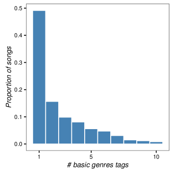
Supplementary Figure 7: Histogram of the number of basic genre tags per song, before filtering. The songs considered for building the histogram are those which have been listened to during the 100 days period under scrutinity.

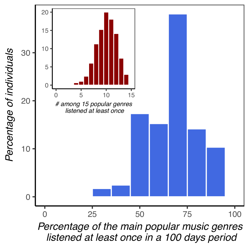
Supplementary Figure 8: Listeners seem eclectic at first sight. Histogram of the proportion of the main genres listened at least once in a 100 days period ; (inset) Histogram of the number of genres listened at least once in a 100 days period among 15 classic popular broad music genres (Pop, Rock, Hip Hop, Dance, R&B/Soul/Funk, Reggae, Electro, Alternative, Country, Jazz, Classical music, Chanson, ’Variété’, Tropical).

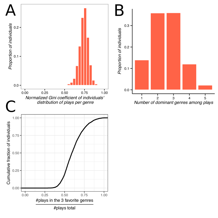
Supplementary Figure 9: The listeners’ inegal repartition of plays among the music genres they listen to. (a) Distribution of the Gini coefficient values of individuals that resume the inequality of their distribution of plays among the different main music genres (b) Histogram of the number of dominant genres $D$ among individuals (see Methods in the main text for details about the calculation of the number of dominant terms in a distribution from its Gini coefficient) (c) CDF of the weight of the 3 favorite genres (determined from the number of plays) among listeners.

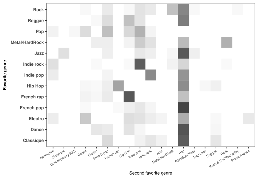
Supplementary Figure 10: Conditional probabilities to observe pairs of favorite genres among listeners. The color intensity of each cell is indexed on the probability $p(g_{2}/g_{1})$ that a listener having $g_{1}$ as favorite genre has $g_{2}$ as second favorite genre.

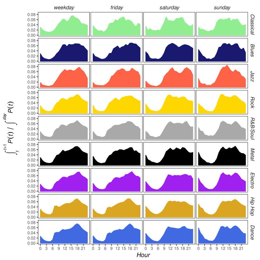
Supplementary Figure 11: Relative proportion of plays as a function of the hour of the day and day of the week, for different music genres. Let alone micro variations – which might be due to the relatively small number of listeners of certain genres at certain hours (nb: the total number of listeners under study is 4615) and to statistical fluctuations – we see no significative differences between the average listening time profiles of the genres.

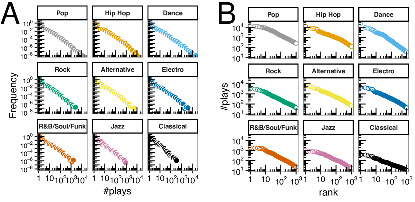
Supplementary Figure 12: The hierarchy of songs in various genres. (a) Histogram of the number of plays per song for the same set of genres (b) Rank-size plot for the 1000 most popular songs in the streams of nine classic music genres.

Supplementary Figure 13: Exploration statistics for groups of fans of various music genres, along with the average age of the group members (fill colour) and its importance among the population of listeners (circle size).

References

- (1) Theodor W. Adorno. On the Fetish-Character in Music and the Regression of Listening. Zeitschrift für Sozialforschung, 7, 1938.
- (2) Philippe Le Guern and Hugh Dauncey, editors. Stereo: Comparative Perspectives on the Sociological Study of Popular Music in France and Britain. Routledge, Farnham, Surrey, England ; Burlington, VT, December 2010.
- (3) Pierre Bourdieu. Distinction: A Social Critique of the Judgement of Taste. Harvard University Press, 1984.
- (4) George Carney. Music Geography. Journal of Cultural Geography, 18(1):1–10, September 1998.
- (5) Conrad Lee and Padraig Cunningham. The Geographic Flow of Music. In Proceedings of the 2012 International Conference on Advances in Social Networks Analysis and Mining (ASONAM 2012), ASONAM ’12, pages 691–695, Washington, DC, USA, 2012. IEEE Computer Society.
- (6) Nik Cohn. Awopbopaloobop Alopbamboom: The Golden Age of Rock. Grove Press, New York, 1972.
- (7) Peter Guralnick. Sweet Soul Music: Rhythm And Blues And The Southern Dream Of Freedom. Canongate Books, 1986.
- (8) Raymond AK Cox, James M. Felton, and Kee H. Chung. The concentration of commercial success in popular music: An analysis of the distribution of gold records. Journal of cultural economics, 19(4):333–340, 1995.
- (9) Juan Prieto-Rodríguez and Víctor Fernández-Blanco. Are Popular and Classical Music Listeners the Same People? Journal of Cultural Economics, 24(2):147–164, May 2000.
- (10) J. A. Sloboda. Everyday Uses of Music Listening: A Preliminary Study. In S.W. Yi, editor, Music, Mind & Science, pages 354–369. Seoul National University Press, 1999.
- (11) Adrian C. North, David J. Hargreaves, and Susan A. O’Neill. The importance of music to adolescents. British Journal of Educational Psychology, 70(2):255–272, June 2000.
- (12) Dave Miranda and Michel Claes. Music listening, coping, peer affiliation and depression in adolescence. Psychology of Music, 37(2):215–233, January 2009.
- (13) Susan Hallam, Ian Cross, and Michael Thaut. Oxford Handbook of Music Psychology. Oxford University Press, May 2011.
- (14) Daniel J. Levitin. This Is Your Brain on Music: The Science of a Human Obsession. Dutton, 2006.
- (15) Valorie N. Salimpoor, Mitchel Benovoy, Gregory Longo, Jeremy R. Cooperstock, and Robert J. Zatorre. The Rewarding Aspects of Music Listening Are Related to Degree of Emotional Arousal. PLOS ONE, 4(10):e7487, October 2009.
- (16) Nick Prior. Critique and Renewal in the Sociology of Music: Bourdieu and Beyond. Cultural Sociology, 5(1):121–138, January 2011.
- (17) Bethany Bryson. ”Anything But Heavy Metal”: Symbolic Exclusion and Musical Dislikes. American Sociological Review, 61(5):884–899, 1996.
- (18) Koen van Eijck. Social Differentiation in Musical Taste Patterns. Social Forces, 79(3):1163–1185, March 2001.
- (19) Patrik N. Juslin and Petri Laukka. Expression, Perception, and Induction of Musical Emotions: A Review and a Questionnaire Study of Everyday Listening. Journal of New Music Research, 33(3):217–238, September 2004.
- (20) Amanda E. Krause, Adrian C. North, and Lauren Y. Hewitt. Music-listening in everyday life: Devices and choice. Psychology of Music, August 2013.
- (21) Teresa Lesiuk. The effect of music listening on work performance. Psychology of Music, 33(2):173–191, January 2005.
- (22) Nicola Dibben and Victoria J. Williamson. An exploratory survey of in-vehicle music listening. Psychology of Music, 35(4):571–589, January 2007.
- (23) Suvi Saarikallio. Music as emotional self-regulation throughout adulthood. Psychology of Music, 39(3):307–327, October 2010.
- (24) Liila Taruffi and Stefan Koelsch. The Paradox of Music-Evoked Sadness: An Online Survey. PLOS ONE, 9(10):e110490, October 2014.
- (25) David M. Greenberg, Simon Baron-Cohen, David J. Stillwell, Michal Kosinski, and Peter J. Rentfrow. Musical Preferences are Linked to Cognitive Styles. PLOS ONE, 10(7):e0131151, July 2015.
- (26) Tom F. M. Ter Bogt, Juul Mulder, Quinten A. W. Raaijmakers, and Saoirse Nic Gabhainn. Moved by music: A typology of music listeners. Psychology of Music, 39(2):147–163, January 2011.
- (27) Thomas Schäfer. The Goals and Effects of Music Listening and Their Relationship to the Strength of Music Preference. PLOS ONE, 11(3):e0151634, March 2016.
- (28) R. Lambiotte and M. Ausloos. Uncovering collective listening habits and music genres in bipartite networks. Physical Review E, 72(6):066107, December 2005.
- (29) Patricia Sarran. Baromètre musicusages (annual report on contemporary listening practices). Syndicat National de l’édition Phonographique, 2016. available online at http://www.snepmusique.com/actualites-du-snep/barometre-musicusages-le-premier-tableau-de-bord-de-la-consommation-de-musique-en-ligne/.
- (30) Albert-László Barabási. The origin of bursts and heavy tails in human dynamics. Nature, 435(7039):207–211, 2005.
- (31) Maxime Lenormand, Miguel Picornell, Oliva Garcia Cantú-Ros, Antònia Tugores, Thomas Louail, Ricardo Herranz, Marc Barthelemy, Enrique Frías-Martínez, and José J. Ramasco. Cross-Checking Different Sources of Mobility Information. PLoS ONE, 9(8):e105184, August 2014.
- (32) Maxime Lenormand, Thomas Louail, Oliva Garcia Cantú Ros, Miguel Picornell, Ricardo Herranz, Juan Murillo Arias, Marc Barthelemy, Maxi San Miguel, and José J. Ramasco. Influence of sociodemographics on human mobility. Scientific Reports, 5:10075, May 2015.
- (33) Paul Lamere. Exploring age-specific preferences in listening. Music Machinery blog post. https://musicmachinery.com/2014/02/13/age-specific-listening/
- (34) Geoffray Bonnin and Dietmar Jannach. Automated Generation of Music Playlists: Survey and Experiments. ACM Comput. Surv., 47(2):26:1–26:35, November 2014.
- (35) M. Jagger and K. Richards. You can’t always get what you want. In Let It Bleed. Decca, 1969.
- (36) F. Sinatra. In the Wee Small Hours. Capitol, 1955.
- (37) Albert LeBlanc, Young Chang Jin, Lelouda Stamou, and Jan McCrary. Effect of Age, Country, and Gender on Music Listening Preferences. Bulletin of the Council for Research in Music Education, (141):72–76, 1999.
- (38) Mohsen Kamalzadeh, Dominikus Baur, and Torsten Möller. Listen or interact? A Large-scale survey on music listening and management behaviours. Journal of New Music Research, 45(1):42–67, January 2016.
- (39) Colin Jerolmack and Shamus Khan. Talk is cheap ethnography and the attitudinal fallacy. Sociological Methods & Research, 43(2):178–209, 2014.
- (40) Alinka E. Greasley and Alexandra Lamont. Exploring engagement with music in everyday life using experience sampling methodology. Musicae Scientiae, 15(1):45–71, March 2011.
- (41) Spotify Insights. https://insights.spotify.com
- (42) Paul Lamere. The Skip. Music Machinery blog post, https://musicmachinery.com/2014/05/02/the-skip/
- (43) Kevin Lewis. Three fallacies of digital footprints. Big Data & Society, 2(2):2053951715602496, December 2015.
- (44) Riccardo Gallotti, Armando Bazzani, Sandro Rambaldi, and Marc Barthelemy. A stochastic model of randomly accelerated walkers for human mobility. Nature Communications, 7:12600, August 2016.