How close are time series to power tail Lévy diffusions?

Abstract

This article presents a new and easily implementable method to quantify the so-called coupling distance between the law of a time series and the law of a differential equation driven by Markovian additive jump noise with heavy-tailed jumps, such as $\alpha$-stable Lévy flights. Coupling distances measure the proximity of the empirical law of the tails of the jump increments and a given power law distribution. In particular they yield an upper bound for the distance of the respective laws on path space. We prove rates of convergence comparable to the rates of the central limit theorem which are confirmed by numerical simulations. Our method applied to a paleoclimate time series of glacial climate variability confirms its heavy tail behavior. In addition this approach gives evidence for heavy tails in data sets of precipitable water vapor of the Western Tropical Pacific.

Keywords: Time series analysis; Statistics of Markovian jump diffusions; Power law distributions; Lévy flights; Wasserstein distance;

1 Introduction

Understanding the nature of noise in data is of paramount interest in nonlinear dynamics in order to build statistically trustworthy models, whose study leads to relevant new theoretical insights. In this context stochastic modeling consists in the study of deterministic and stochastic differential equations, which represent on the one hand the mechanistic understanding of the underlying phenomenon and on the other different kinds of noise accounting the effect of unresolved processes. In various applications the fluctuations present in time series of interest exceed the plausible thresholds for an underlying Gaussian white noise perturbation. The continuity of Markovian Gaussian models given as stochastic differential equations makes it necessary to go beyond the Gaussian paradigm to model random fluctuations and to include the effect of shocks. A natural class of Markovian perturbations containing discontinuous paths is given by so-called Lévy processes, sometimes referred to as Lévy flights, which are non-Gaussian and discontinuous extensions of Brownian motion which retain the white noise structure of stationary, $\delta$-correlated increments. While some such processes enjoy scaling properties (for instance $\alpha$-stable processes), scaling is not a generic property of Lévy processes, (Section 2).

In this article we present a new statistical method to estimate the proximity of time series to the paths of a given diffusion model with additive jump Lévy noise. In essence this is the comparison (in $L^{2}$-sense) of a discrete approximation of a path and “typical” paths of such a model. We stress that the path-wise comparison is the strongest possible form of comparison between stochastic processes. Our method consists of two steps.

The first step in this method uses our main theoretical result (provided in [17]), which states that the distance of the paths can be estimated using so-called coupling distances between the underlying Lévy jump measures. This distance, which compares the distributions of instantaneous jump increments of the processes, is based on appropriately scaled Wasserstein distances. Wasserstein distances between two probability distributions are well-known in the mathematics literature [33] and measure the “optimal $L^{2}$ transport” between the two distributions. In other words, they minimize on the product space the deviation from the diagonal (in $L^{2}$-sense) over all joint distributions of the two “marginal” distributions. We emphasize that an estimate of the distance of temporal path statistics using a distance only of the instantaneous jump distributions is not entirely straight-forward. First, there are in general infinitely many of such jumps in any finite time interval and the deterministic motion does not mitigate the effect of jumps or can even enhance it. Furthermore, even in the case of finitely many jumps, the jumps of two processes beyond a common threshold typically occur with different intensities. In order to compare such paths with different “random clocks” we have to “synchronize” them in order to compare the jump distributions. As a toy example of our result imagine two compound Poisson processes with joint intensity $\lambda>0$, with different jump distributions $\mu_{1}$ and $\mu_{2}$. Then our main result states that on a finite time horizon the path statistics of these two processes (in the $L^{2}$-norm of the supremum distance) can be estimated using the difference of the coupling distance of $\mu_{1}$ and $\mu_{2}$.

The second step in our method exploits the following advantage of the notion of a coupling-distance. Since its main ingredients are the so-called Wasserstein distances, it is statistically tractable in that we can use well-established results on rates of convergence. In [18] the notion of coupling distance is shown to be weak enough (in a topological sense) to allow for an efficient statistical assessment of a given time series within a class of models. In this study we prove the most relevant version of the original result on the rates of convergence and illustrate these results by using simulations. In Section 4 we demonstrate how the rates of convergence depend on the sample size. The statistical method is particularly useful for the comparison of compound Poisson (finite intensity) processes and for identifying power law distributions in time series, as will be demonstrated using meteorological and climatological examples in Section 5. The first set of time series considered is a the well-studied example of the Greeland Ice Core Project (GRIP) paleoclimatic proxies indicating abrupt transitions between stadials and interstadials of the last glacial period. In [10] Ditlevsen identified an $\alpha$-stable Lévy component in the GRIP calcium concentration record through consideration of the statistics of time series increments. Further investigation in that direction has been carried out in [15] and [21] exploiting the scaling properties of these processes. As a second example we consider long records of precipitable water vapor in the Western Tropical Pacific (Manus and Nauru) which are governed by dynamics with a strong threshold effect and exhibit clearly recognizable heavy-tailed patterns. Our approach is more general than those used previously. In particular, it does not rely on scaling properties of the time series. A preliminary investigation of heavy tail behavior in time series in [18] is systematically extended in this article, resulting in a robust and well-tested tool for the detection of polynomial tails in time series.

The article is organized as follows. In Section 2 we introduce Lévy processes and motivate the notion of Wasserstein distance between probability measures and coupling distance between Lévy measures before stating the main theoretical estimate proved in [17]. In Section 3 we describe the implementation of the coupling distance and derive asymptotic rates of convergence. Section 4 considers the application of the method to synthetic time series, and includes sensitivity analyses related to the data size and model parameters. In Section 5 we analyze climatic time series to assess evidence of heavy tailed behavior.

2 Coupling distances between Lévy measures

2.1 Lévy processes

Lévy processes are the common generalization of Poisson processes and Brownian motion. Both processes have statistically independent and stationary increments. In the case of a Poisson process $P=(P(t))_{t\geqslant 0}$, (with intensity $\lambda>0$) given by $P(t)-P(s)\sim P(t-s)\sim\mbox{Poi}(\lambda(t-s))$, and in the case of a (standard, scalar) Brownian motion $B=(B(t))_{t\geqslant 0}$ with $B(t)-B(s)\sim B(t-s)\sim\mathcal{N}(0,t-s)$. In addition, each of these processes starts at $0$ and has at least right-continuous paths, which enjoy left limits at each point in time $t\geqslant 0$. The concept of a Lévy process lifts the assumption of an explicitly prescribed stationary increment distribution. A Lévy process $L=(L(t))_{t\geqslant 0}$ is a stochastic process starting at $0$ with independent and stationary increments in the sense that $L(t)-L(s)\sim L(t-s)$ and that has trajectories which are right-continuous $L(t+)=L(t)$ and have left limits in each point of time. That is, $L(t-)$ exists, which yields a well-defined jump size $\Delta_{t}L=L(t)-L(t-)$. This type of path yields for each point in time $t$ the decomposition of the current state $L(t)=L(t-)+\Delta_{t}L$ into the “predictable” (that is, continuously accessible) part $L(t-)$ of $L(t)$ (w.r.t. the underlying flow of information) and the “non-anticipating” jump increment $\Delta_{t}L$ of $L(t)$ (w.r.t. the underlying flow of information). The jump increment is statistically independent from $L(s)$ for all $s<t$ and hence also of $L(t-)$ due to the independence of increments. Lévy processes are well-studied objects in the mathematics literature.

The so-called Lévy-Itô decomposition states that any given Lévy process $L=(L(t))_{t\geqslant 0}$ in $\mathbb{R}^{k}$ can be decomposed path-wise into the sum of the following four unique and independent components

$$L(t)=at+A^{1/2}B(t)+C(t)^{\rho}+J^{\rho}(t)\qquad\leavevmode\nobreak\ \mbox{ for all }\leavevmode\nobreak\ t\geqslant 0\quad\mathbb{P}-\mbox{a.s.}$$ (1)

The vector $a\in\mathbb{R}^{k}$ accounts for the linear drift, $B=(B(t))_{t\geqslant 0}$ is a $d$-dimensional standard Brownian motion, which comes with a non-negative definite, symmetric covariance matrix $A\in\mathbb{R}^{d\otimes d}$. The processes $(C^{\rho}(t))_{t\geqslant 0}$ and $(J^{\rho}(t))_{t\geqslant 0}$ are pure jump processes which share as a common parameter the so-called Lévy measure $\nu$ and a threshold $\rho>0$. The Lévy measure $\nu$ is given as a sigma-finite measure on the Borel sets $\nu:\mathfrak{B}(\mathbb{R}^{k})\rightarrow[0,\infty]$ satisfying for any $\rho>0$ that

$$\nu(\{0\})=0,\qquad\int_{\mathcal{B}_{\rho}(0)}|x|^{2}\nu(dx)<\infty\qquad\mbox{ and }\qquad\nu(\mathbb{R}^{k}\setminus\mathcal{B}_{\rho}(0))<\infty,$$ (2)

where $\mathcal{B}_{\rho}(0)=\{y\in\mathbb{R}^{k}\leavevmode\nobreak\ |\leavevmode\nobreak\ |y|<\rho\}$. For each fixed $\rho>0$ the measure $\nu$ parametrizes two associated processes in the following way. The first process, $C^{\rho}=(C^{\rho}(t))_{t\geqslant 0}$, is a compound Poisson process with Poisson jump intensity $\lambda_{\rho}=\nu(\mathbb{R}^{k}\setminus\mathcal{B}_{\rho}(0))$ and jump distribution $\nu_{\rho}$

$$\mathfrak{B}(\mathbb{R}^{k})\ni E\mapsto\nu_{\rho}(E):=\frac{\nu(E\cap(\mathbb{R}^{k}\setminus\mathcal{B}_{\rho}(0)))}{\lambda_{\rho}}.$$ (3)

That is, $C^{\rho}$ is a Markovian pure jump process with memoryless and hence exponentially distributed waiting times between consecutive jumps of intensity $\lambda_{\rho}$, which are independent and distributed according to $\nu_{\rho}$ in (3). Note that the jumps of $C^{\rho}$ are bounded away from zero by $\rho$. The second process is another Markovian pure jump process $J^{\rho}=(J^{\rho}(t))_{t\geqslant 0}$, whose jumps are bounded from above by $\rho$ with possibly infinite intensity. The process $(J^{\rho}(t))_{t\geqslant 0}$ can be understood as follows. The Fourier transform of the marginal law $L_{t}$ is given by the so-called Lévy-Chinchine decomposition

$$\mathbb{E}[\exp(i\langle u,L(t)\rangle)]=\exp(t\Psi(u)),\qquad t\geqslant 0,u\in\mathbb{R}^{k},$$

with

$$\Psi(u)=i\langle u,a\rangle-\frac{1}{2}\langle a,Aa\rangle+\int_{\mathbb{R}^{k}\setminus\mathcal{B}_{\rho}(0)}\big{[}e^{i\langle u,y\rangle}-1\big{]}\nu(dy)+\int_{\mathcal{B}_{\rho}(0)}\big{[}e^{i\langle u,y\rangle}-1-i\langle u,y\rangle\big{]}\nu(dy),\qquad u\in\mathbb{R}^{k}.$$

This representation tells us that $J^{\rho}=(J^{\rho}(t))_{t\geqslant 0}$ can be understood as the superposition of independent compensated (i.e. re-centered) compound Poisson processes $J^{\rho}(t)=\sum_{j=1}^{\infty}(\tilde{C}^{j}(t)-t\int_{R_{j}}y\nu(dy))$, where the compound Poisson processes $\tilde{C}^{j}$ take jumps with values in rings given by $R_{j}=\{\rho_{j}<|y|\leqslant\rho_{j-1}\}$, distributed as $E\mapsto\frac{\nu(E\cap R_{j})}{\nu(R_{j})}$ with intensity $\nu(R_{j})<\infty$. The sequence $\rho=\rho_{0}>\rho_{1}>\dots>0$ of radii is strictly decreasing and $\rho_{j}\searrow 0$ such that $\mathcal{B}_{\rho}(0)\setminus\{0\}=\bigcup_{j\in\mathbb{N}_{0}}R_{j}$ with joint (possibly infinite) intensity

$$\sum_{j\in\mathbb{N}_{0}}\nu(R_{j})=\nu(\mathcal{B}_{\rho}(0))\leqslant\infty.$$

Note that if the total jump intensity $\nu(\mathcal{B}_{\rho}(0))<\infty$ we can choose $\rho=0$ and hence $J^{\rho}\equiv 0$.

The case of $\alpha$-stable processes:

The physically most familiar class of Lévy processes beyond the Poisson process and Brownian motion are the so-called stable processes, sometimes also referred to as Lévy flights. They have a parameter $\alpha\in(0,2)$ and enjoy the following scaling property

$$\frac{1}{c^{\frac{1}{\alpha}}}L(ct)\stackrel{{\scriptstyle d}}{{=}}L(t),\qquad\mbox{ for all }c>0\mbox{ and }t\geqslant 0.$$

$\alpha$-stable processes are pure jump processes of infinite intensity with the heavy-tailed Lévy measure

$$\nu(dz)=\frac{c_{-}}{|z|^{1+\alpha}}\mathbf{1}\{z<0\}+\frac{c_{+}}{z^{1+\alpha}}\mathbf{1}\{z>0\}.$$ (4)

such that $c_{+}+c_{-}>0$. We make the following remarks on basic properties of $\alpha$-stable processes:

1. The situation that $c_{-}\neq c_{+}$ implies that the Lévy measure is asymmetric and also produces asymmetric $\alpha$-stable marginal laws, which however turn out to be still self-similar. For more on this property we refer to Sato [35].

2. The marginal distributions have all smooth densities. Closed forms of the densities however are only known in special cases. For instance the $(\alpha=1)$-stable process is known to be necessarily symmetric $c=c_{-}=c_{+}$ and is given by the standard Cauchy process.

3. All $\alpha$-stable processes are pure jump processes and only allow finite moments of order $p<\alpha<2$, as is evident from the equivalent integrability condition $\int_{|z|>1}|z|^{p}\nu(dz)<\infty$.

4. The degenerate case of a strictly asymmetric Lévy measure (4) given for instance for $c_{-}=0$ and $c_{+}=1$ yields a jump process with jumps only in positive direction. In this case the $\alpha=\frac{1}{2}$-stable Lévy process is called the Lévy subordinator. It can be constructed as the random clock given as the points in time that a Brownian motion $B$ catches up with the linear function $t\mapsto t/\sqrt{2}$

   $$t\mapsto T_{t}:=\inf\{s>0\leavevmode\nobreak\ |\leavevmode\nobreak\ B(s)>\frac{t}{\sqrt{2}}\}.$$

   For further details on the distribution and density on this relation we refer to [35].

5. The limiting case of $\alpha=2$ is also necessarily symmetric and corresponds to a Brownian motion. However Brownian motion enjoys very different properties than stable processes for parameter $0<\alpha<2$. For instance, it has continuous sample paths and exponential moments.

2.2 Coupling distance

The standard case of the coupling distance between Lévy measures:

In the article [17] the authors construct a special metric, the so-called coupling distance, on the set of Lévy measures $\nu$ in $\mathbb{R}^{k}$. This metric exploits the fact that for any $\rho>0$ the tail-measure $\nu_{\rho}$ as defined before is a probability measure. Hence, having two Lévy processes $L$ and $L^{\prime}$ with Lévy measures $\nu$ and $\nu^{\prime}$, the basic idea is now to find cutoffs $\rho$ and $\rho^{\prime}$ such that the intensities $\lambda_{\rho}$ and $\lambda^{\prime}_{\rho^{\prime}}$ are equal, that is the $C^{\rho}$ and $C^{\prime\rho^{\prime}}$ have the same intensity. Then, to compare the jump measures it is natural to compare the probability measures $\nu_{\rho}$ and $\nu^{\prime}_{\rho}$, which we will denote by $\mu$ and $\mu^{\prime}$ for short.

The Wasserstein distance:

In our case the comparison of two given probability distributions $\mu$ and $\mu^{\prime}$ relies on the so-called Wasserstein distance between $\mu$ and $\mu^{\prime}$ on $\mathbb{R}^{k}$. For the construction of the Wasserstein distance between $\mu$ and $\mu^{\prime}$ we consider all joint distributions $\Pi$ on the product space $\mathbb{R}^{k}\times\mathbb{R}^{k}$ having these two marginal distributions, that is $\Pi(E\times\mathbb{R}^{k})=\mu(E)$ and $\Pi(\mathbb{R}^{k}\times E)=\mu^{\prime}(E)$ for any $E\in\mathcal{B}(\mathbb{R}^{k})$. If $\mu=\mu^{\prime}$, then the special joint distribution $\Pi(E\times E^{\prime})=\mu(E\cap E^{\prime})$ concentrates all the mass on the diagonal $\{(x,x)\leavevmode\nobreak\ |\leavevmode\nobreak\ x\in\mathbb{R}^{k}\}$ of the product space. In particular the mean-square of the distance from the diagonal $\int_{\mathbb{R}^{k}\times\mathbb{R}^{k}}|x-y|^{2}\Pi(dx,dy)=0$. If $\mu\neq\mu^{\prime}$ there is obviously not such a joint distribution, that is $\int_{\mathbb{R}^{k}\times\mathbb{R}^{k}}|x-y|^{2}\Pi(dx,dy)>0$. However, it turns out to be a good measure of proximity of $\mu$ and $\mu^{\prime}$ to minimize over all joint distributions or couplings of $\mu$ and $\mu^{\prime}$ given by

$$\mathfrak{C}(\mu,\mu^{\prime}) :=\Big{\{}\Pi:\mathfrak{B}(\mathbb{R}^{k})\otimes\mathfrak{B}(\mathbb{R}^{k})\rightarrow[0,1]\mbox{ probability measure, with }$$

$$\qquad\leavevmode\nobreak\ \Pi(E\times\mathbb{R}^{k})=\mu(E),\quad\Pi(\mathbb{R}^{k}\times E)=\mu^{\prime}(E)\quad\mbox{ for all }E\in\mathfrak{B}(\mathbb{R}^{k})\Big{\}}.$$ (5)

The Wasserstein metric of order $2$ between two probability measures $\mu,\mu^{\prime}$ on the Borel sets of $\mathbb{R}^{k}$ is defined by

$$W_{2}(\mu,\mu^{\prime}):=\inf_{\Pi\in\mathfrak{C}(\mu,\mu^{\prime})}\Big{(}\int_{\mathbb{R}^{k}\times\mathbb{R}^{k}}|x-y|^{2}\Pi(dx,dy)\leavevmode\nobreak\ \Big{)}^{\frac{1}{2}}.$$

Any minimizer $\Pi^{*}$ is referred to as optimal coupling between $\mu$ and $\mu^{\prime}$. It is obvious that in terms of random vectors $(X,X^{\prime})$ with $X\sim\mu$ and $X^{\prime}\sim\mu^{\prime}$ and joint distribution $\Pi$ the Wasserstein-distance has the following equivalent form

$$W_{2}(\mu,\mu^{\prime}):=\inf_{\begin{subarray}{c}\Pi\in\mathfrak{C}(\mu,\mu^{\prime})\\ (X,X^{\prime})\sim\Pi\end{subarray}}\mathbb{E}_{\Pi}\big{[}|X-X^{\prime}|^{2}\big{]}^{\frac{1}{2}}.$$

Properties of the Wasserstein distance:

It is well-known in the mathematics literature [33] that the convergence $W_{2}(\mu_{n},\mu)\rightarrow 0$ is equivalent to the weak convergence of the laws $\mu_{n}\rightharpoonup\mu$, that is, the convergence $\mu_{n}(B)\longrightarrow\mu(B)$ for all “reasonable” events $B$ and the convergence of the second moments. In this work we will consider the following case. The optimal coupling between $\mu$ and $\mu^{\prime}$ is not in general known explicitly, with the notable exception of $k=1$, where a parametrization of the optimal coupling $\Pi$ is given as follows. On $(\mathbb{R},|\cdot|)$ one can show that for two distribution functions $F(x)=\mu((-\infty,x])$ and $F^{\prime}(x)=\mu^{\prime}((-\infty,x])$ the optimal coupling is realized by the random vector

$$(X,Y)=(F^{-1}(U),(F^{\prime})^{-1}(U)),$$ (6)

where $F^{-1}$ and $(F^{\prime})^{-1}$ are the quantile functions of $F$ and $F^{\prime}$ and $U$ has the uniform distribution in $[0,1]$. Therefore the Wasserstein metric is easily evaluated by

$$W_{2}^{2}(\mu,\mu^{\prime})=\int_{0}^{1}|(F^{-1}(u)-(F^{\prime})^{-1}(u)|^{2}du.$$ (7)

It is worth noting that the optimality of the pair $(X,Y)$ holds only with respect to the specific (spatial) metric $d(x,y)=|x-y|$ on $\mathbb{R}$. The law of $(X,Y)$ is obviously a coupling of $\mu$ and $\mu^{\prime}$. For metrics other than $d$ the right-hand side of (7) is in general an upper bound. If we consider the Wasserstein distance for other metric, such as the cut-off metric $d_{s}(x,y)=\min(|x-y|\wedge s)$ for some $s>0$ on $\mathbb{R}$, we lose the result that the specific coupling (6) is minimal. However, since the Wasserstein distance is given as the infimum over all couplings with respect to $d$ the means square distance with (6) yields at least an upper bound. The real line with the cut-off metric $d_{s}$ will be the space where we approximate the laws of the jumps, since we are considering processes which may not have second moments. For further results we refer to [17] and [18].

Note that Wasserstein distances can be considered on much more general spaces than $\mathbb{R}^{k}$. For instance consider two stochastic processes $(X̣^{j}_{t})_{t\in[0,1]}$ with continuous trajectories, so $\mbox{Law}(X^{j})$ is a distribution on $(\mathcal{C}([0,1]),\mathcal{B}(\mathcal{C}([0,1]))$. Then

$$W_{2}(\mu,\mu^{\prime})=\inf_{\Pi\in\mathfrak{C}(\mu,\mu^{\prime})}\Big{(}\int_{\mathcal{C}([0,1])\times\mathcal{C}([0,1])}d(x,y)^{2}\Pi(dx,dy)\leavevmode\nobreak\ \Big{)}^{\frac{1}{2}}$$

is well-defined in the usual sense, where $d(x,y)$ is any complete metric in $\mathcal{C}([0,1])$, for instance $d(x,y)=\|x-y\|_{\infty}=\sup_{t\in[0,1]}|x(t)-y(t)|$ or $d(x,y)=\|x-y\|_{\infty}\wedge s=\sup_{t\in[0,1]}d_{s}(x(t),y(t))$. The same is true for the more general space $\mathbb{D}([0,1])$ of right-continuous functions with left limits $v:[0,1]\rightarrow\mathbb{R}$, that is satisfying $v(t+)=v(t)$ and $v(t-)\in\mathbb{R}$ for any $t\in[0,1]$. This is the natural space in which Lévy processes in the sense of (1) have their paths. Analogously to the case of continuous functions, the Wasserstein distance is well-defined. For instance, for two Lévy processes $L$ and $L^{\prime}$ the Wasserstein distance between their laws $\mu=\mbox{Law}(L)$ and $\mu^{\prime}=\mbox{Law}(L^{\prime})$ in $\mathbb{D}([0,1])$ is given by

$$W_{2,d}(\mu,\mu^{\prime})=\inf_{\Pi\in\mathfrak{C}(\mu,\mu^{\prime})}\Big{(}\int_{\mathbb{D}([0,1])\times\mathbb{D}([0,1])}d(x,y)^{2}\Pi(dx,dy)\leavevmode\nobreak\ \Big{)}^{\frac{1}{2}}$$ (8)

using for identical metrics $d$ as before.

The definition of the coupling semimetric and the coupling distance, standard case:

We are now in the position to define the coupling semimetric family and the coupling distance between two Lévy measures $\nu$ and $\nu^{\prime}$.

Definition 2.1

Given two absolutely continuous Lévy measures $\nu=fdx$ and $\nu^{\prime}=f^{\prime}dx$ on $\mathbb{R}^{k}$ and a given intensity $0<\lambda<\min(\nu(\mathbb{R}^{k}),\nu^{\prime}(\mathbb{R}^{k}))$ we define the cutoffs

$$\rho(\lambda):=\inf\{r>0\leavevmode\nobreak\ |\leavevmode\nobreak\ \nu(\mathbb{R}^{k}\setminus\mathcal{B}_{r}(0))\leqslant\lambda\}$$

and $\rho^{\prime}(\lambda)$ analogously. We then introduce a family of semi-metrics $T_{\lambda}$

$$T_{\lambda}(\nu,\nu^{\prime}):=\lambda^{\frac{1}{2}}\;W_{2}(\nu_{\rho(\lambda)},\nu^{\prime}_{\rho^{\prime}(\lambda)}).$$

First note that the absolute continuity yields that given $\nu$ and intensity $\lambda>0$ we have that the mass of the Lévy measure outside $\rho(\lambda)$ is just $\lambda$, that is formally $\lambda_{\rho(\lambda)}=\lambda$, with $\lambda_{\rho}$ defined before (3). Intuitively, given Lévy measures $\mu$ and $\mu^{\prime}$, the semi-metric $T_{\lambda}(\nu,\nu^{\prime})$ compares the jump distributions $\nu_{\rho(\lambda)}$ and $\nu^{\prime}_{\rho^{\prime}(\lambda)}$ of two compound Poisson processes with common intensity $\lambda=\lambda_{\rho(\lambda)}=\lambda_{\rho^{\prime}(\lambda)}$.

A word about the renormalization pre-factor $\lambda^{\frac{1}{2}}$: roughly speaking, it comes from the fact that an increasing intensity $\lambda$ makes the cutoffs $\rho$ approach $0$. However around $0$ the Lévy measure has a well-known “worst-case” pole associated with the integrability condition $\int_{-1}^{1}z^{2}\nu(dz)<\infty$ of the Lévy-Chinchine decomposition, which has to be satisfied for any Lévy measure. The pre-factor $\lambda^{1/2}$ allows the coupling distance to remain finite even for large $\lambda$. We illustrate why this is the case using the one-sided Lévy measure $\nu(dz)=\frac{dz}{|z|^{1+\alpha}}\mathbf{1}_{(0,1)}(z)$, $z\in(0,1)$ for some $\alpha\in(0,2)$. In this case we have $\nu(0,1)=\infty$. Consider now two Lévy measures $\nu,\nu^{\prime}$ of this type with exponents $\alpha,\alpha^{\prime}\in(0,2)$. Calculating their optimal coupling explicitly we observe the following. For given intensity $\lambda\gg 1$ we calculate the cutoff $\rho$ of $\nu$ as

$$\lambda=2\int_{\rho}^{1}\frac{dz}{z^{1+\alpha}}=\frac{2}{\alpha}\Big{(}\frac{1}{\rho^{\alpha}}-1\Big{)}\quad\Leftrightarrow\quad\rho=\Big{(}\frac{2}{2+\alpha\lambda}\Big{)}^{\frac{1}{\alpha}}.$$

Hence the tail distribution function and the quantile function satisfy

$$F_{\rho}(x)=\nu_{\rho}([x,1))=\frac{1}{\lambda}\int_{x}^{1}\frac{dz}{z^{1+\alpha}}=\frac{1}{\lambda}\frac{2}{\alpha}\Big{(}\frac{1}{x^{\alpha}}-1\Big{)}\mbox{ for }\leavevmode\nobreak\ \rho\leqslant x<1\qquad\mbox{ and hence}$$

$$F_{\rho}^{-1}(y)=\Big{(}\frac{2}{\lambda\alpha y+2}\Big{)}^{\frac{1}{\alpha}}=\lambda^{-\frac{1}{\alpha}}\Big{(}\frac{\frac{2}{\alpha}}{y+\frac{2}{\alpha}\frac{1}{\lambda}}\Big{)}^{\frac{1}{\alpha}}.$$

Analogously we obtain ${\nu^{\prime}}_{\rho^{\prime}}$ and ${F^{\prime}}_{\rho^{\prime}}^{-1}(y)$ and calculate with the help of the triangular inequality for $L^{2}(0,1)$ and a standard expansion for large $\lambda\gg 1$

$$\lambda^{\frac{1}{2}}\mathcal{W}_{2}(\nu_{\rho},{\nu^{\prime}}_{\rho^{\prime}}) =\Big{(}\int_{0}^{1}\lambda(F_{\rho}^{-1}(y)-{F^{\prime}}_{\rho^{\prime}}^{-1}(y))^{2}dy\Big{)}^{\frac{1}{2}}$$

$$=\Big{(}\int_{0}^{1}\Big{[}\lambda^{\frac{1}{2}-\frac{1}{\alpha}}\Big{(}\frac{\frac{2}{\alpha}}{y+\frac{2}{\alpha}\frac{1}{\lambda}}\Big{)}^{\frac{1}{\alpha}}-\lambda^{\frac{1}{2}-\frac{1}{\alpha^{\prime}}}\Big{(}\frac{\frac{2}{\alpha^{\prime}}}{y+\frac{2}{\alpha^{\prime}}\frac{1}{\lambda}}\Big{)}^{\frac{1}{\alpha^{\prime}}}\Big{]}^{2}dy\Big{)}^{\frac{1}{2}}$$

$$\leqslant\lambda^{\frac{1}{2}-\frac{1}{\alpha}}\Big{(}\int_{0}^{1}\Big{(}\frac{\frac{2}{\alpha}}{y+\frac{2}{\alpha}\frac{1}{\lambda}}\Big{)}^{\frac{2}{\alpha}}dy\Big{)}^{\frac{1}{2}}+\lambda^{\frac{1}{2}-\frac{1}{\alpha^{\prime}}}\Big{(}\int_{0}^{1}\Big{(}\frac{\frac{2}{\alpha^{\prime}}}{y+\frac{2}{\alpha^{\prime}}\frac{1}{\lambda}}\Big{)}^{\frac{2}{\alpha^{\prime}}}dy\Big{)}^{\frac{1}{2}}$$

$$\stackrel{{\scriptstyle\lambda\gg 1}}{{\approx}}\lambda^{\frac{1}{2}-\frac{1}{\alpha}}\lambda^{1-\frac{2}{\alpha}}+\lambda^{\frac{1}{2}-\frac{1}{\alpha^{\prime}}}\lambda^{1-\frac{2}{\alpha^{\prime}}}=\lambda^{3(\frac{1}{2}-\frac{1}{\alpha})}+\lambda^{3(\frac{1}{2}-\frac{1}{\alpha^{\prime}})}.$$

Since $\alpha,\alpha^{\prime}<2$ we obtain that even for this worst case pole around $0$ there the function $\lambda\mapsto\lambda^{\frac{1}{2}}\mathcal{W}_{2}(\nu_{\rho},{\nu^{\prime}}_{\rho^{\prime}})$ is asymptotically decreasing, and hence globally bounded. Taking the supremum over all $\lambda>0$ is hence a meaningful operation.

Note further that the bivariate function $T_{\lambda}$ is symmetric and satisfies the triangle inequality hence it is a semi-metric. Clearly, $T_{\lambda}(\nu,\nu^{\prime})=0$ does not guarantee that $\nu=\nu^{\prime}$, since the values of $\nu|_{B_{\rho(\lambda)}}$ are not taken into account. Therefore it is not a proper metric despite being symmetric and satisfying the triangular inequality. For details we refer [17].

To overcome the shortcomings of using a semi-metric we take the following approach. We assume that the Lévy measure has a density with respect to the Lebesgue measure and that it has infinite mass $\nu(\mathbb{R}^{k})=\infty$. Hence, the cut-off as a function of the intensity $\lambda\mapsto\rho(\lambda)$ is continuous and monotonically decreasing with $\lim_{\lambda\rightarrow\infty}\rho(\lambda)=0$: the set of increments not taken into account by the semi-metric $T_{\lambda}$ given by $B_{\rho(\lambda)}(0)$ is strictly decreasing. Therefore it makes sense to take as a distance between two Lévy measures the supremum $T_{\lambda}$ over all $\lambda>0$.

Definition 2.2

For two absolutely continuous Lévy measures $\nu=fdx$ and $\nu^{\prime}=f^{\prime}dx$ on $\mathbb{R}^{k}$ with $\nu(\mathbb{R}^{k})=\nu^{\prime}(\mathbb{R}^{k})=\infty$ we define the coupling distance

$$T(\nu,\nu^{\prime}):=\sup_{\lambda>0}T_{\lambda}(\nu,\nu^{\prime}).$$

We stress that both the restrictions of absolutely continuous measures and infinite activity in the definition above can be removed. For details we refer to the original work [17]. On the one hand the restriction on absolute continuity is overcome by an interpolation procedure. The requirement of infinite mass can be dropped by the ad hoc introduction of an artificial point mass in $0$ carrying the missing weight. In this way, finite Lévy measures are accommodated in this framework. We also refer to [18], for further applications of coupling distances.

Coupling distances between Lévy measures, the general case:

The fact that a finite Wasserstein distance and hence finite coupling distance require finite second moments implies that coupling distances between $\alpha$-stable Lévy measures are not yet covered by Definition 2.2. In order to treat the distance between $\alpha$-stable Lévy SDEs, we slightly modify the definition of $T_{\lambda}$ and $T$ with the help of the truncated Wasserstein distance. For $s>0$ given we define

$$\tilde{W}_{2,s}^{2}(\mu,\mu^{\prime})=\inf_{\Pi\in\mathfrak{C}(\mu,\mu^{\prime})}\Big{(}\int_{\mathbb{R}\times\mathbb{R}}(|x-y|^{2}\wedge s)\leavevmode\nobreak\ \Pi(dx,dy)\leavevmode\nobreak\ \Big{)}^{\frac{1}{2}}$$

and analogously

$$\tilde{T}_{\lambda}(\nu,\nu^{\prime})=\lambda^{\frac{1}{2}}\tilde{W}_{2,s}^{2}(\nu_{\rho(\lambda)},\nu^{\prime}_{\rho^{\prime}(\lambda)}),\qquad\tilde{T}(\nu,\nu^{\prime})=\sup_{\lambda>0}T_{\lambda}(\nu,\nu^{\prime}).$$

This truncation allows us to measure the proximity of Lévy measures. While small values $|x-y|\leqslant\sqrt{s}$ are unaffected, large values of $|x-y|$, which violate the square integrability are set equal to a constant. As a result, $\tilde{T}_{\lambda}(\nu,\nu^{\prime})\leqslant(\lambda s)^{\frac{1}{2}}$. Clearly, the coupling (6) is no longer the optimal coupling for the modified Wasserstein distance $\tilde{W}_{2}^{2}$, which cannot be evaluated analogously to (7). However, for the following truncated version of (7)

$$\tilde{W}_{2,s}^{2}(\mu,\mu^{\prime})\leqslant\int_{0}^{1}\Big{(}|(F^{-1}(u)-(F^{\prime})^{-1}(u)|^{2}\wedge s\Big{)}du,$$ (9)

the Wasserstein distance given as minimal coupling of this cutoff distance is less than equal to the given coupling on the right hand side of equation 7.

2.3 The central estimates

We now turn to the estimates of the Wasserstein distance of the laws of two solutions of stochastic differential equations driven by different Lévy noise processes on path space, making use of standard distances on the parameters including the coupling distance between the underlying Lévy measures. Note that from now on we will work throughout the text with non-dimensionalized quantities. This is justified later on in Section 4 by the scaling property of our estimator shown in Figure 5. In principal the scale used for non-dimensionalization is arbitrary. In our analysis, we will focus on the interquartile range as this is defined for all random variables.

We consider two stochastic differential equations $j=1,2$ of the following type

$$X_{j}(t)=x_{j}+\int_{0}^{t}f\left(X_{j}(s)\right)ds+L_{j}(t)\qquad t\geqslant 0,\leavevmode\nobreak\ x_{j}\in\mathbb{R}.$$ (10)

where each $L_{j}$ is a Lévy process in the sense of (1) with the characteristic triplet $(a_{j},A_{j},\nu_{j})$ and the vector field $f:\mathbb{R}\rightarrow\mathbb{R}$ is continuous and satisfies the following monotonicity condition

$$(f(x)-f(y))(x-y)\leqslant\ell(x-y)^{2},\quad x,y\in\mathbb{R},\mbox{ for some }\ell>0.$$ (11)

It is well-known that unique strong Markovian solutions to (10) are obtained analogously to ordinary differential equations via a Picard - type successive iteration procedure.

Generic examples satisfying (11) are all globally Lipschitz continuous functions and polynomials of odd order with negative leading coefficient

$$f(x)=b_{n}x^{n}+\sum_{i=0}^{n-1}b_{i}x^{i},\qquad b_{n}<0,\leavevmode\nobreak\ b_{i}\in\mathbb{R},\leavevmode\nobreak\ n\mbox{ odd}.$$

In applications such a polynomial is often considered as the gradient $f=-U^{\prime}$ of an energy potential $U:\mathbb{R}\rightarrow\mathbb{R}$ with several local minima. In climate science a class of such examples examples can be derived from radiative energy balance considerations ([3], [25], [24], [10] and references therein). Under the proper choice of parameters the potential $U$ admits two local minima that correspond to two climate equilibrium states (we refer to the discussion in Section 5.1). In neuroscience the FitzHugh-Nagumo model is an example of such a fourth order potential $U$. In this case equation (10) models the membrane voltage under random excitation, which has been studied recently in the literature (e.g. [4], [11], [39]).

The first of our main theoretical results estimates the deviation between the laws of the solutions $X_{j}$ on $(\mathbb{D}(0,1),\tilde{d})$ in terms of the metric induced by $T$ and $T_{\lambda}$ on the set of tupel of parameters $(x_{j},a_{j},A_{j},\nu_{j})$.

Theorem 2.1

Let $f:\mathbb{R}\rightarrow\mathbb{R}$ be $\mathcal{C}^{2}$ and satisfy condition (11) for some constant $\ell>0$ and $(a_{j},A_{j},\nu_{j})$ be two Lévy characteristics and given initial values $x_{j}\in\mathbb{R}$, $j=1,2$.

Then for any two solutions $X_{j}$ of equation (10) driven by Lévy processes $L_{j}$ with the respective characteristics there are uniform constants $c_{1},c_{2}>0$ such that

$$\mathcal{W}_{2,\tilde{d}}^{2}\Big{(}\mathrm{Law}(X_{1}),\mathrm{Law}(X_{2})\Big{)}\leqslant c_{1}\;Q^{1}e^{\ell/\arctan(1/2)}+c_{2}\;Q^{2},$$ (12)

where $\mathcal{W}_{2,d}$ is the Wasserstein distance on the path space $\mathbb{D}([0,1])$ equipped with the cutoff metric $\tilde{d}(g,h):=\|g-h\|_{\infty}\wedge s$ in the sense of (8) and

$$Q^{1} =|x_{1}-x_{2}|^{2}\wedge s+|a_{1}-a_{2}|+(\sqrt{A_{1}}-\sqrt{A_{2}}\,)^{2}+T^{2}(\nu_{1},\nu_{2})$$

$$\quad+\big{(}\nu_{1}(|u|>s)+\nu_{2}(|u|>s)\big{)}^{1/2}T(\nu_{1},\nu_{2}),$$

$$Q^{2} =\sqrt{(\sqrt{A_{1}}-\sqrt{A_{2}})^{2}+T^{2}(\nu_{1},\nu_{2})}.$$

This result states that the Wasserstein distance of the optimal paths in the function space $\mathbb{D}([0,1])$ (that is for all $t\in[0,1]$ simultaneously) is estimated by the distances of the characteristics of the marginals $L^{j}_{t}$, which are identical for all $t\in[0,1]$. In addition, the Wasserstein distances on the right-hand side are between Lévy measures in $\mathbb{R}$, such that the optimal coupling is either known (in the case without cutoff $s=\infty$) or can be estimated in the case $s<\infty$. This result is the strongest possible since it compares the mean-square of the paths uniformly on a given time interval. The proof of this result is a consequence of the following more technical but practically much more useful result, which includes the choice of a level of intensity $\lambda$ and the estimation of $\mathcal{W}_{2,\tilde{d}}(\mathrm{Law}(X_{1}),\mathrm{Law}(X_{2}))$ by a respective semi-metric $T_{\lambda}$. In addition, all constants are given explicitly. This result is primarily of theoretical value as it is impossible in practice to evaluate the coupling distance simultaneously for all intensities $\lambda>0$, since this requires an arbitrarily large number of data points. Therefore we state a simpler version for fixed finite intensity $\lambda>0$. Since we work with non-dimensionalized data it is enough to state the following result with $s=1$.

Theorem 2.2

Let $f:\mathbb{R}\rightarrow\mathbb{R}$ be $\mathcal{C}^{2}$ and satisfy condition (11) for some constant $\ell>0$ and $(a_{j},A_{j},\nu_{j})$ be two Lévy characteristics and given initial values $x_{j}\in\mathbb{R}$, $j=1,2$. In addition, let the expression $\mathcal{W}_{2,\tilde{d}}$ be defined as in Theorem 2.1.

Then for any $\lambda>0$ and any two solutions $X_{j}$ of equation (10) driven by Lévy processes $L_{j}$ with the respective characteristics the following estimate holds true

$$\mathcal{W}_{2,\tilde{d}}^{2}\Big{(}\mathrm{Law}(X_{1}),\mathrm{Law}(X_{2})\Big{)} \leqslant Q_{\lambda}^{1}e^{\ell/C_{0}}+Q_{\lambda}^{2},$$

where

$$Q_{\lambda}^{1} =2(|x_{1}-x_{2}|^{2}\wedge 1)+C_{1}\Big{(}C_{2}|a_{1}-a_{2}|+(\sqrt{A_{1}}-\sqrt{A_{2}}\,)^{2}+U_{\lambda}\left(\nu_{1}\right)+U_{\lambda}\left(\nu_{2}\right)+$$

$$\quad+C_{3}T^{2}_{\lambda}(\nu_{1},\nu_{2})+C_{4}\min(\nu_{1}(|u|>1)+\nu_{2}(|u|>1),\lambda)^{1/2}T_{\lambda}(\nu_{1},\nu_{2})\Big{)},$$

$$Q_{\lambda}^{2} =C_{1}\sqrt{C_{5}(\sqrt{A_{1}}-\sqrt{A_{2}})^{2}+C_{6}(U_{\lambda}\left(\nu_{1}\right)+U_{\rho}\left(\nu_{2}\right)+T^{2}_{\lambda}(\nu_{1},\nu_{2}))},$$

$$U_{\lambda}\left(\nu_{j}\right)=\int_{|u|\leqslant\rho_{j}(\lambda)}u^{2}\nu_{j}(du),\qquad j=1,2,$$

with the following numerical values.

Constant	$C_{0}$	$C_{1}$	$C_{2}$	$C_{3}$	$C_{4}$	$C_{5}$	$C_{6}$
Exact value	$\arctan(1/2)$	$4/\pi$	$3^{3/4}/2$	$\pi+3^{3/4}$	$(\pi+3^{3/4})/2$	$3^{3/2}$	$(2\pi)^{2}$
Numerical approx.	$0.46$	$1.27$	$1.40$	$5.42$	$2.28$	$5.20$	$39.48$

3 Statistical implementation and rates of convergence

In this section we develop a practical implementation of the program laid out in the previous sections. In order to keep both calculations and strategy tractable we will restrict ourselves to a simple example, which can be adapted and extended. While this section has some overlap with Section 3 in [18] we present a simplified and streamlined version of the proof of the rates of convergence. We start with some basic statistics and the implementation of the sample Wasserstein distance between the empirical measure and reference measures. With these tools at hand we prove rates of convergence for the sample distance. In the last subsection we explain our procedure in detail.

3.1 Basic statistics

In this section we provide the technical background to compare the jump statistics of a data set to a given reference distribution in terms of the coupling distance. Since our focus is essentially one dimensional we concentrate on the scalar case. For higher dimensions we refer to the Conclusion.

3.1.1 Basic notions and results

For a given sequence of independent and identically distributed random variables $(X_{i})_{i\in\mathbb{N}}$ with distribution $\mu$ on $\mathbb{R}$ we denote by $\mu_{n}$ the empirical distribution based on the sample of size $n$ defined as

$$\mu_{n}(E):=\frac{\#\{X_{i}\in E\}}{n}=\frac{1}{n}\sum_{i=1}^{n}\mathbf{1}{\{X_{i}\in E\}}\ ,\quad E\in\mathfrak{B}(\mathbb{R})\ .$$ (13)

The corresponding empirical distribution function $F_{n}$ is the distribution function of $\mu_{n}$

$$F_{n}(x):=\mu_{n}((-\infty,x])=\frac{\#\{X_{i}\leqslant x\}}{n}=\frac{1}{n}\sum_{i=1}^{n}\mathbf{1}{\{X_{i}\leqslant x\}}\ ,\quad x\in\mathbb{R}\ .$$ (14)

A version of the strong law of large numbers known as the Glivenko-Cantelli Theorem tells us that for the distribution function $F(x)=\mu((-\infty,x])$, $x\in\mathbb{R}$, of $\mu$ we have for almost all $\omega\in\Omega$ the uniform convergence

$$\sup_{x\in\mathbb{R}}|F_{n}(x,\omega)-F(x)|\to 0\quad\mbox{ as }n\to\infty\ .$$ (15)

Non-trivial limits of the quantity in (15) are obtained by the following rescaling. For any fixed $x\in\mathbb{R}$, the random variables $\mathbf{1}\{X_{i}\leqslant x\}$, $i\in\mathbb{N}$ are i.i.d. Bernoulli variables with $F(x)=\mathbb{P}(X_{i}\leqslant x)$. Hence the central limit theorem (de Moivre-Laplace Theorem) states that

$$\sqrt{n}\left(F_{n}(x)-F(x)\right)=\frac{1}{\sqrt{n}}\sum_{i=1}^{n}\mathbf{1}\{X_{i}\leqslant x\}-\sqrt{n}F(x)\stackrel{{\scriptstyle d}}{{\longrightarrow}}\mathcal{N}\left(0,F(x)(1-F(x))\right).$$ (16)

Quantiles:

To compute the Wasserstein distance it is necessary to consider the empirical quantile function $F_{n}^{-1}$. For $n\in\mathbb{N}$ denote by $X_{i:n}$ the $i$-th order statistic of a sample of size $n$, i.e. $i$-th smallest element of the the ordered sample

$$X_{1:n}\leqslant\dots\leqslant X_{i:n}\leqslant\cdots\leqslant X_{n:n}.$$

The quantile $F_{n}^{-1}$ of $F_{n}$ can then be expressed in terms of the order statistics since for $0<u\leqslant 1$

$$\begin{split}F_{n}^{-1}(u)&=\inf\{x\in\mathbb{R}:\ F_{n}(x)\geqslant u\}=\inf\{x\in\mathbb{R}:\#\{X_{i}\leqslant x\}\geqslant nu\}=X_{\lceil nu\rceil:n}\ .\end{split}$$ (17)

In analogy to (15) the strong law of large numbers implies that

$$|F^{-1}_{n}(u,\omega)-F^{-1}(u)|\rightarrow 0\ ,\qquad\mbox{ for all }u\in(0,1)\mbox{ as }n\rightarrow\infty\mbox{ for almost all }\omega\in\Omega.$$

However, in general we cannot expect uniform convergence in $u$, since unbounded support of $\mu$ implies that the values of the quantile $F^{-1}(u)$ for $u$ tending to $0,1$ will tend to infinity. To obtain the analogy to the central limit theorem of formula (16) we introduce the well-known concept in time series analysis of empirical quantile process.

Definition 3.1

Let $(X_{i})_{i\in\mathbb{N}}$ be a sequence of real valued i.i.d. random variables with common distribution function $F$. The empirical quantile process is defined as

$$Q_{n}(u,\omega):=\sqrt{n}\left(F^{-1}_{n}(u,\omega)-F^{-1}(u)\right),\quad 0\leqslant u\leqslant 1,\ n\in\mathbb{N}\ .$$ (18)

For $\mu$ being the uniform distribution we obtain the following analogue of the central limit theorem.

Theorem 3.1

Let $(X_{i})_{i\in\mathbb{N}}$ be a sequence of real valued i.i.d. random variables with common uniform distribution function $F(x)=x$, $x\in[0,1]$. Then there exists a Brownian bridge $(B^{0}_{n})_{n\in\mathbb{N}}$, that is a Brownian motion conditioned to end in $0$ at the endpoint $x=1$, such that

$$\sup_{0\leqslant u\leqslant 1}|Q_{n}(u,\omega)-B^{0}_{u}(\omega)|\stackrel{{\scriptstyle d}}{{\longrightarrow}}0,\mbox{ as }n\rightarrow\infty.$$ (19)

As already mentioned, for general distributions $F$ uniform convergence of the empirical quantile process is unavailable. Instead, we will consider truncated $L^{2}$ distances later. In the following we link the empirical quantile process to the approximation of Wasserstein distances.

3.1.2 The implementation of the empirical Wasserstein distance

We measure the speed of convergence described by the Glivenko-Cantelli theorem in terms of the Wasserstein distance as follows.

The Wasserstein distance between the empirical measure and the reference measure:

For some given reference distribution $\mu$ with second moments we calculate the Wasserstein distance between an empirical measure $\mu_{n}(\omega)$ and $\mu$ itself. For convenience let us introduce the Wasserstein statistic with respect to $d(x,y)=|x-y|$

$$\operatorname{\mathrm{w}_{n}}:=\operatorname{\mathrm{w}_{n}}(\mu,\omega):=W_{2}^{2}(\mu_{n}(\omega),\mu),\qquad\mbox{ for }n\in\mathbb{N}.$$ (20)

This distance can be calculated explicitly due to the explicitly known shape of the optimal coupling by

$$\operatorname{\mathrm{w}_{n}}=\int_{0}^{1}|F_{n}^{-1}(u)-F^{-1}(u)|^{2}du=\int_{0}^{1}|X_{\lceil nu\rceil:n}-F^{-1}(u)|^{2}du\\ =\sum_{i=1}^{n}\int_{\frac{i-1}{n}}^{\frac{i}{n}}(X_{(i-1):n}-F^{-1}(u))^{2}du.$$ (21)

The expression on the right side of (21) turns out to be a second order polynomial in the order statistic, that is

$$\operatorname{\mathrm{w}_{n}}=\sum_{i=1}^{n}a_{i}X_{i:n}^{2}+b_{i}X_{i:n}+c\ ,$$ (22)

where the coefficients are determined by the binomial formula and given by

$$a_{i}=\frac{1}{n},\quad b_{i}=-2\int_{\frac{i-1}{n}}^{\frac{i}{n}}F^{-1}(u)du,\quad c=\int_{0}^{1}\big{(}F^{-1}(u)\big{)}^{2}du\ .$$ (23)

The cutoff Wasserstein distance between the empirical measure and the reference measure:

The previous result can also be adapted for the cut-off version. In this case we consider the Wasserstein distance with respect to $d(x,y)=|x-y|\wedge s$ for some cutoff $s>0$. For simplicity in this context (and because in practice we will work with non-dimensionalized time series) we restrict ourselves in the discussion to the case of $s=1$. Other cutoff values are implemented analogously. Note that in the cutoff case the optimal coupling is no longer explicit, however the analogous measure $|F_{n}^{-1}(u)-F^{-1}(u)|\wedge 1$ remains a (generally suboptimal) coupling. Therefore the Wasserstein distance with respect to $d(x,y)=|x-y|\wedge 1$ satisfies

$$W_{2}^{2}(\mu_{n},\mu)\leqslant\int_{0}^{1}\big{(}|F_{n}^{-1}(u)-F^{-1}(u)|\wedge 1\big{)}^{2}du=:\operatorname{\mathrm{w}_{n}^{*}}(\mu)=:\operatorname{\mathrm{w}_{n}^{*}}\ ,$$ (24)

where the right-hand side can be calculated similarly to (22) in terms of the order statistics as follows

$$\operatorname{\mathrm{w}_{n}^{*}}=\sum_{i=1}^{n}A_{i}X_{i:n}^{2}+B_{i}X_{i:n}+C_{i}+D.$$ (25)

For the repartition $0\leqslant\ell_{1}\leqslant r_{1}\leqslant\ell_{2}\leqslant r_{2}\leqslant\cdots\leqslant\ell_{n}\leqslant r_{n}\leqslant 1$ given by

$$\ell_{i}=\left(\frac{i-1}{n}\vee|F(X_{i:n}-1)|\right)\wedge\frac{i}{n}\ ,\qquad r_{i}=\frac{i-1}{n}\vee\left(|F(X_{i:n}+1)|\wedge\frac{i}{n}\right)$$ (26)

the coefficients are calculated by

$$A_{i}=r_{i}-\ell_{i},\quad B_{i}=-2\int_{\ell_{i}}^{r_{i}}F^{-1}(u)du,\quad C_{i}=\int_{\ell_{i}}^{r_{i}}\big{(}F^{-1}(u)\big{)}^{2}du,\quad D=1-\sum_{i=1}^{n}A_{i}\ .$$ (27)

3.2 Asymptotic distribution and rate of convergence for power laws

For rigorous statistical applications it is necessary to determine the rate of convergence of the statistic of interest, in our case $\operatorname{\mathrm{w}_{n}^{*}}$. By definition $\operatorname{\mathrm{w}_{n}^{*}}$ tends to zero as $n\rightarrow\infty$. Quantifying the rate of convergence amounts to finding the correct renormalization to obtain a non-trivial (random) limit. For calculational convenience we state the theorem for the one-sided case. The negative tail is chosen so that for a given density $f$ the function $f(F^{-1})$ is again monotonically increasing. The two-sided case is a straight-forward extension as the sum of both one-sided coupling distances.

Theorem 3.2

Assume $f(x)=c^{\alpha}|x|^{-\alpha-1}$ for all $x<-c$ and some $\alpha>0$. Then for any $\kappa$ with

$$0<\kappa<\frac{\alpha}{\alpha+2}\ ,$$

there exists a sequence of non-negative random variables $(\mathcal{E}_{\kappa,n})_{n\in\mathbb{N}}$ (on the same probability space) such that for all $n\in\mathbb{N}$

$$n^{\kappa}\;\operatorname{\mathrm{w}_{n}}^{*}\leqslant\;\mathcal{E}_{\kappa,n}\qquad\mbox{$\mathbb{P}-$almost surely,}$$

which converges in distribution

$$\mathcal{E}_{\kappa,n}\stackrel{{\scriptstyle d}}{{\longrightarrow}}c^{2}\int_{0}^{1}(u^{\frac{1}{\alpha}-1}B_{u})^{2}du\quad{as}\quad n\rightarrow\infty\ ,$$

where $B=(B_{u})_{u\in[0,1]}$ is a standard Brownian motion.

Proof: First consider a sequence of deterministic intermediate points $(k_{n})_{n\in\mathbb{N}}$ such that

$$1\leqslant k_{n}\leqslant n\quad\mbox{satisfying }\quad k_{n}\nearrow\infty\ \quad\mbox{ and }\quad n^{\kappa-1}{k_{n}}\searrow 0\quad\mbox{ as }n\to\infty\ .$$

For instance, we can choose $k_{n}=n^{\gamma}$ for any $0<\gamma<1-\kappa$. We then estimate

$$n^{\kappa}\operatorname{\mathrm{w}_{n}}^{*}=n^{\kappa}\int_{0}^{1}\Big{(}|F_{n}^{-1}(u)-F^{-1}(u)|^{2}\wedge 1\Big{)}du \leqslant n^{\kappa-1}{k_{n}}+n^{\kappa}\int_{\frac{k_{n}}{n}}^{1}\Big{(}|F_{n}^{-1}(u)-F^{-1}(u)|^{2}\Big{)}du=:\mathcal{E}_{\kappa,n}\ .$$ (28)

The first term vanishes asymptotically by assumption. The integral component of $\mathcal{E}_{\kappa,n}$ is then split into the integrals from $\frac{k_{n}}{n}$ to $\frac{1}{2}$ and from $\frac{1}{2}$ to $1$. The first integral is treated with the help of Theorem 2.4 in [8]. With a slight adaption to our situation it states precisely that for the quantile process $Q_{n}(u)$ of the uniform distribution on $[0,1]$, given by Definition 3.1 as $Q_{n}(u)=\sqrt{n}(U_{n}^{-1}(u)-u)$, and any $\eta>1$ we have the following limit in distribution

$$\Big{(}\frac{k_{n}}{n}\Big{)}^{2(\eta-1)}\int_{\frac{k_{n}}{n}}^{\frac{1}{2}}\Big{(}\frac{Q_{n}(u)}{u^{\eta}}\Big{)}^{2}du\stackrel{{\scriptstyle d}}{{\longrightarrow}}\int_{0}^{1}u^{2\eta-4}|B_{u}|^{2}du\quad{as}\quad n\rightarrow\infty.$$ (29)

The mean value theorem tells us that for some (random) intermediate value $\vartheta_{n}(u)$ satisfying

$$u\wedge U_{n}(u)\leqslant\vartheta_{n}(u)\leqslant u\vee U_{n}(u)$$ (30)

we have for each $\omega\in\Omega$

$$n\int_{\frac{k_{n}}{n}}^{\frac{1}{2}}\Big{(}|F_{n}^{-1}(u)-F^{-1}(u)|^{2}\Big{)}du =n\int_{\frac{k_{n}}{n}}^{\frac{1}{2}}\bigg{(}\Big{(}\frac{\partial}{\partial u}F^{-1}(\vartheta_{n}(u))\Big{)}^{2}|U_{n}^{-1}(u)-U^{-1}(u)|^{2}\bigg{)}du$$

$$=\int_{\frac{k_{n}}{n}}^{\frac{1}{2}}\Big{(}\frac{|\sqrt{n}(U_{n}^{-1}(u)-u)|^{2}}{f(F^{-1}(\vartheta_{n}(u))^{2}}\Big{)}du$$

$$=\int_{\frac{k_{n}}{n}}^{\frac{1}{2}}\Big{(}\frac{Q_{n}(u)^{2}}{f(F^{-1}(\vartheta_{n}(u))^{2}}\Big{)}du.$$

By means of the facts $f(F^{-1}(u))=c^{-1}u^{1+\frac{1}{\alpha}}$ for $u\in[0,1]$ and $\eta=1+\frac{1}{\alpha}$, the bound (30) and the limit (29) yields

$$n\Big{(}\frac{k_{n}}{n}\Big{)}^{2/\alpha}\int_{\frac{k_{n}}{n}}^{\frac{1}{2}}\Big{(}|F_{n}^{-1}(u)-F^{-1}(u)|^{2}\Big{)}du =\Big{(}\frac{k_{n}}{n}\Big{)}^{2/\alpha}c^{2}\int_{\frac{k_{n}}{n}}^{\frac{1}{2}}\Big{(}\frac{Q_{n}(u)^{2}}{\vartheta_{n}(u)^{2(1+\frac{1}{\alpha})}}\Big{)}du$$ (31)

$$\leqslant\Big{(}\frac{k_{n}}{n}\Big{)}^{2/\alpha}c^{2}\int_{\frac{k_{n}}{n}}^{\frac{1}{2}}\Big{(}\frac{Q_{n}(u)}{(u\wedge U_{n})^{(1+\frac{1}{\alpha})}}\Big{)}^{2}du$$

$$\stackrel{{\scriptstyle d}}{{\longrightarrow}}c^{2}\int_{0}^{1}u^{2(\frac{1}{\alpha}-1)}|B_{u}|^{2}du.$$

Analogously to the above we obtain

$$n\int_{\frac{1}{2}}^{1}\Big{(}|F_{n}^{-1}(u)-F^{-1}(u)|^{2}\Big{)}du =n\int_{\frac{1}{2}}^{1}\bigg{(}\Big{(}\frac{\partial}{\partial u}F^{-1}(\vartheta_{n}(u))\Big{)}^{2}|U_{n}^{-1}(u)-U^{-1}(u)|^{2}\bigg{)}du$$

$$\leqslant\int_{\frac{1}{2}}^{1}\Big{(}\frac{|\sqrt{n}(U_{n}^{-1}(u)-u)|^{2}}{f(F^{-1}(\vartheta_{n}(u))^{2}}\Big{)}du.$$

$$\leqslant c^{2}(\vartheta_{n}(\tfrac{1}{2}))^{-2(1+\frac{1}{\alpha})}\int_{\frac{1}{2}}^{1}\Big{(}\sqrt{n}(U_{n}^{-1}(u)-u)\Big{)}^{2}du$$

$$\stackrel{{\scriptstyle d}}{{\longrightarrow}}c^{2}(\tfrac{1}{2})^{-2(1+\frac{1}{\alpha})}\int_{\frac{1}{2}}^{1}|B^{0}_{u}|^{2}du<\infty\ ,$$

where we used the monotonicity of $f(F^{-1}(u))$ and Theorem 3.1 (Glivenko-Cantelli). $\blacksquare$

This theorem provides an upper bound for the coupling distance between the empirical law of $\mu$-distributed i.i.d. random variables with empirical measures $\mu_{n}$ and the distribution $\mu$ where they are drawn from. The mathematical formulation tells us that we can expect rates of convergence for any $\kappa\in(0,\frac{\alpha}{\alpha+2})$ in our simulation studies compare the empirical rate of convergence to the fastest rate of convergence of order $\frac{\alpha}{\alpha+2}$.

3.3 An overview of the estimation procedure

Since the data of many real-world phenomena exhibit strong fluctuations in relatively short time, it is reasonable to extend stochastic models of continuous evolution to models with jumps. The easiest case to consider is a process of the type

$$Y(t)=G(t)+L(t),\qquad t\in[0,T]\mbox{ for fixed }T>0,$$ (32)

where $G=(G(t))_{t\in[0,T]}$ is a continuous process and $L=(L(t))_{t\in[0,T]}$ is a purely discontinuous Lévy process. We have seen in Section 2 that $L$ is determined by a Lévy triplet of the form $(0,0,\nu)$, where $\nu$ is a Lévy measure defined in (2). For instance, the solutions of stochastic differential equations

$$Y(t)=x+\int_{0}^{t}f(Y(s))ds+L(t),\qquad t\in[0,T],$$

for globally Lipschitz continuous functions $f:\mathbb{R}\rightarrow\mathbb{R}$ fall into this class. The aim of this procedure is to determine the nature of $L$ and thus of its Lévy measure $\nu$.

Given a data set $y=(y_{i})_{i=0,\dots n}$ from a time series the first step of our method consists in a non-dimensionalization of the data. A natural choice for the size of fluctuations is given by the interquartile range, through which we divide throughout this study. This procedure has the particular advantage that it allows us to compare different (non-dimensionalized) time series to the same class of Lévy diffusions. We interpret the given time series $y$ as a realization of a (non-dimensionalized) process $Y$ given in the class of models (32) observed at discrete times $t_{1}<\dots<t_{i}<\dots<t_{n}$, that is

$$y_{i}=Y(t_{i},\omega)\qquad\mbox{ for some }\omega\in\Omega.$$

The following modeling assumptions determine the relation between the observed data and the underlying model. For any fixed threshold $\rho>0$:

1. The observation frequency is sufficiently high in comparison to the occurrence of large jumps given as increments beyond our threshold $\rho$ in that in each observed time interval $[t_{i-1},t_{i})$ at most one large jump occurs. That is, we do not see the sum of two or more large sums.

2. The behavior of small jumps is sufficiently benign in comparison to the large jump threshold $\rho$ during our observation. In particular, we assume that over one time interval $[t_{i-1},t_{i})$ small jump and continuous contributions cannot accumulate to this threshold and appear in the data as a large jump.

These assumptions can be made rigorous by further model assumptions on $Y$, such as the Lipschitz continuity of $G$. Under the modeling assumptions it is justified to estimate jumps by increments

$$Y(t_{i})-Y(t_{i-1})\approx C^{\rho}(s)-C^{\rho}(s-0)\quad\mbox{ for exactly one }s\in[t_{i-1},t_{i}),$$

for the compound Poisson process $C^{\rho}$ given by equation (1), of the jumps of $L$ with $|\Delta_{t}L|>\rho$. Hence the increments $Y(t_{i})-Y(t_{i-1})$ can be considered as the realization of an i.i.d. sequence $X=(X_{i})_{i=1,\dots,n}$ with some common law $\mu$ (concentrated on $\mathbb{R}\setminus(-\rho,\rho)$). We denote by $x=(x_{i})_{i=1,\dots n}$ the vector of large increments

$$x_{i}=(y_{i}-y_{i-1})\mathbf{1}\{|y_{i}-y_{i-1}|>\rho\}$$

so that

$$x_{i}=X_{i}(\omega)\qquad\mbox{ for some }\omega\in\Omega.$$

Let $\mu_{n}$ be the empirical measure of the data $X$ with respect to the common law $\mu$. The Glivenko-Cantelli theorem (14) tells us that for almost all $\omega\in\Omega$

$$\mu_{n}(\omega,\cdot)\rightarrow\mu\qquad n\rightarrow\infty,\mbox{ weakly. }$$

Since by construction $\mu=\nu_{\rho}$ we obtain that $\mu_{n}(\omega)$ converges to $\nu_{\rho}$ weakly. Since the Wasserstein distance encoded in the coupling distance metrizes the weak convergence we have for almost all $\omega\in\Omega$

$$T_{\lambda_{\rho}}(\mu_{n},\nu_{\rho})\rightarrow 0\qquad\mbox{ as }n\rightarrow\infty.$$ (33)

In particular we have an estimator for the tail of the Lévy measure $\nu_{\rho}$. We are now in the position to estimate the distance between the Lévy measure of the compound Poisson approximation $C^{\rho}$ of $L$ (respectively $Y$) with the true but unknown tail measure $\nu_{\rho}$ and the tail $\nu^{*}_{\rho^{*}}$ of a proposed Lévy measure $\nu^{*}$. In particular we obtain

$$T_{\lambda_{\rho^{*}}^{*}}(\nu^{*},\nu_{\rho})\leqslant T_{\lambda_{\rho}^{*}}(\nu^{*}_{\rho},\mu_{n})+T_{\lambda_{\rho^{*}}^{*}}(\mu_{n},\nu_{\rho})\leqslant(\lambda_{\rho^{*}}^{*}\operatorname{\mathrm{w}_{n}}^{*}(\mu_{n},\nu^{*}))^{\frac{1}{2}}+T_{\lambda_{\rho^{*}}^{*}}(\nu_{\rho},\mu_{n}).$$ (34)

The last term on the right-hand side tends to $0$ by (33) with the rate of convergence given in Theorem 3.2 in Subsection 3.2, while the first term can be calculated explicitly due to Section 3.1.2.

The first modeling assumption requires that the rate of jumps is relatively rare, we can achieve this by specifying $\lambda=1$. This requirement along with the test model $\nu^{*}$ determines $\rho^{*}$.

We point out that the term on the left-hand side of equation (34) is an upper bound in Theorem 2.1 for the comparison between two models in the following sense. Under the interpretation that our data stem from a pure jump diffusion $X^{i}$ ($a_{i}=0$ and $A_{i}=0$) with (unknown) Lévy measure $\nu$ we can compare its paths to the paths of the proposed model $\nu^{*}$ and quantify the corresponding coupling distances.

4 Simulation studies

4.1 Rates of convergence for small observation lengths

In Subsection 3.2 we obtained upper bounds for the asymptotic rate of convergence of the statistic $\operatorname{\mathrm{w}_{n}}^{*}(\mu)$ defined in (24) for large values of $n$. This section illustrates by means of simulations that the estimation procedure is unbiased and that the asymptotic rate of convergence for large $n$ holds approximately for small sample sizes driven by processes with power-law tails.

We consider a parametrized compound Poisson process $C_{t}$ with unit intensity and polynomial jump distribution of order $\alpha_{0}$. More precisely we assume that each jump is distributed according to $\nu^{\alpha_{0}}$, where

$$\nu^{\alpha}(dz)=\begin{cases}(\alpha\rho_{0}^{\alpha})\frac{\displaystyle dz}{\displaystyle z^{1+\alpha}},&z\geqslant\rho_{0}\\ 0,&z<\rho_{0}\end{cases}.$$ (35)

We fix $\rho_{0}=0.5$. Then for each given tail index parameter $\alpha_{0}\in\left\{1.4,1.8,3.0\right\}$ we simulate a sample of $m=100$ sample paths. For each single sample path we evaluate the upper bound of the random function $\alpha\mapsto W_{2}(\nu^{\alpha_{0}}_{n}(\omega),\nu^{\alpha})$, given by the random curve

$$\alpha\mapsto\operatorname{\widetilde{\mathrm{w}_{n}}}(\alpha;\alpha_{0})(\omega):=\int_{0}^{1}\big{(}|(F_{n}^{\alpha_{0}}(\omega))^{-1}(u)-(F^{\alpha})^{-1}(u)|\wedge 1\big{)}^{2}du,$$ (36)

for the first $n\in\{10^{2},10^{3},10^{4},10^{5}\}$ points of the sample path. Here, $F_{n}^{\alpha_{0}}(\omega)$ is the empirical distribution function of the first $n$ points of the sample $\omega$ and $(F_{n}^{\alpha_{0}}(\omega))^{-1}(u)$ is its corresponding quantile process, $F^{\alpha}$ is the exact empirical distribution function of $\nu^{\alpha}$ and $(F^{\alpha})^{-1}(u)$ is its corresponding quantile function. Note that for the parameter $\alpha=\alpha_{0}$ we have by construction $\operatorname{\widetilde{\mathrm{w}_{n}}}(\alpha_{0};\alpha_{0})(\omega)=\operatorname{\mathrm{w}_{n}}(\nu^{\alpha_{0}})(\omega)$, as was derived in (20) of Subsubsection 3.1.2, and for which we have obtained the rates of convergence in Subsection 3.2. This way we obtain $4$ sets (one for each value of $n$) of $m=100$ realizations of the curves $\alpha\mapsto\operatorname{\widetilde{\mathrm{w}_{n}}}(\alpha;\alpha_{0})(\omega)$. These curves are shown in Figure 1 (a), (c), (e). Figures 1 (b), (d), (f) show the histograms of the minimum distance estimator $\widehat{\alpha}_{n}$,

$$\widehat{\alpha}_{n}(\omega):=\arg\inf_{\alpha}\left\{\operatorname{\widetilde{\mathrm{w}_{n}}}(\alpha;\alpha_{0})(\omega)\right\}\ ,$$ (37)

indicating how the minima of the curves $\alpha\mapsto\operatorname{\widetilde{\mathrm{w}_{n}}}(\alpha;\alpha_{0})(\omega)$ are distributed around the true value $\alpha_{0}$.

$\longrightarrow$ Position of Figure 1

(a)

(b)

(c)

(d)

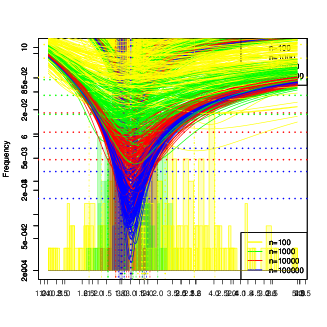
(e)

(f)

Figure 1: Simulations of the empirical distance curves $\alpha\mapsto\operatorname{\widetilde{\mathrm{w}_{n}}}(\alpha;\alpha_{0})$ and the empirical minimal distance estimator $\widehat{\alpha}_{n}$ for distinct values of $\alpha_{0}$: (a) and (b) show $\alpha_{0}=1.4$; (c) and (d) show $\alpha_{0}=1.8$; (e) and (f) show $\alpha_{0}=3.0$.

All sample curves in Figure 1(a),(c),(e) exhibit unique minima distributed around the true value $\alpha_{0}$. It is apparent that the minimum distances decrease with increasing observation length $n$. From Figure 1 (b),(d),(f) it is clear that the empirical distribution of the minimum distance estimator $\widehat{\alpha}_{n}$ is centered at $\alpha_{0}$ with decreasing variance as $n$ increases. This behavior is also seen in Table 1, which displays the empirical mean and empirical variance of the minimum distance estimator $\widehat{\alpha}_{n}$ and the minimum distance statistic $\widehat{\operatorname{\mathrm{w}_{n}}}^{*}$ for the different observation lengths $n$ and $\alpha_{0}$.

In order to compare the empirical and the asymptotic convergence rates of the empirical Wasserstein distance $\widehat{\operatorname{\mathrm{w}_{n}}}^{*}$ to $0$ we compare the sample mean and variance of $\widehat{\operatorname{\mathrm{w}_{n}}}^{*}$ to the asymptotic upper bound for the rate of convergence given in Theorem 3.2. (Tables  2 and 3) By Theorem 3.2 the statistic $\widehat{\operatorname{\mathrm{w}_{n}}}^{*}$ converges for increasing $n$ with order $n^{-\kappa}$, for any $0<\kappa<\frac{\alpha}{\alpha+2}$. It is therefore instructive to compare the convergence of the sample mean of $\widehat{\operatorname{\mathrm{w}_{n}}}^{*}$ to $0$ with $n^{-\frac{\alpha_{0}}{\alpha_{0}+2}}$ on a logarithmic scale. From inspection of the empirical means of $\widehat{\operatorname{\mathrm{w}_{n}}}^{*}$ (the dotted horizontal lines in Figures 1 (a),(c),(e)) it is apparent that the sample means for different powers of 10 are evenly spaced when scaled logarithmically. For increasing power of $10^{i}$, $i=2,\dots,5$ we compare

$$Q_{i,i+1}=\mbox{sample mean}(\widehat{\mathrm{w}_{10^{i+1}}^{*}})/\mbox{sample mean}(\widehat{\mathrm{w}_{10^{i}}^{*}})$$

with the respective power of $10^{-\frac{\alpha_{0}}{\alpha_{0}+2}}$ (Table 2). For the small values of $\alpha_{0}=1.4$ and $\alpha_{0}=1.8$ we obtain already for small sample sizes a reasonably good scaling. For $\alpha_{0}=3.0$ the empirical ratio is of the same order of magnitude but larger than the asymptotic one. The linear scaling of the standard deviation of $\hat{w^{*}}$ makes it appropriate to compare the analogous quantity

$$R_{i,i+1}=\sqrt{\mbox{sample var}(\widehat{\mathrm{w}_{10^{i+1}}^{*}})/\mbox{sample var}(\widehat{\mathrm{w}_{10^{i}}^{*}})}$$

for the (sample) standard variation with the same quantity $10^{-\frac{\alpha_{0}}{\alpha_{0}+2}}$. We see a reasonable fit of the scaling factors for $\alpha_{0}=1.4$ and $\alpha_{0}=1.8$ and larger errors for $\alpha_{0}=3.0$. This overall picture indicates that the asymptotic rates of convergences are attained faster for smaller values of $\alpha_{0}$.

$\longrightarrow$ Position of Table 1

$$\begin{array}[]{ll|ll|ll|ll|ll}&&&n=10^{2}&&n=10^{3}&&n=10^{4}&&n=10^{5}\\ \alpha_{0}&&\widehat{\alpha}_{n}&\widehat{\operatorname{\mathrm{w}_{n}}^{*}}&\widehat{\alpha}_{n}&\widehat{\operatorname{\mathrm{w}_{n}}^{*}}&\widehat{\alpha}_{n}&\widehat{\operatorname{\mathrm{w}_{n}}^{*}}&\widehat{\alpha}_{n}&\widehat{\operatorname{\mathrm{w}_{n}}^{*}}\\ \hline\cr 1.4&\text{mean}&1.48&1.30\times 10^{-1}&1.40&4.74\times 10^{-2}&1.40&1.83\times 10^{-2}&1.40&6.63\times 10^{-3}\\ &\text{var}&3.67\times 10^{-3}&2.71\times 10^{-3}&2.34\times 10^{-3}&2.02\times 10^{-4}&3.94\times 10^{-4}&2.86\times 10^{-5}&6.48\times 10^{-5}&3.99\times 10^{-6}\\ \hline\cr 1.8&\text{mean}&1.95&8.80\times 10^{-2}&1.81\times 10^{-2}&3.03\times 10^{-2}&1.81&1.05\times 10^{-2}&1.80&3.40\times 10^{-3}\\ &\text{var}&6.03\times 10^{-2}&1.54\times 10^{-2}&5.31\times 10^{-3}&0.12\times 10^{-3}&0.81\times 10^{-3}&1.37\times 10^{-5}&0.20\times 10^{-3}&1.29\times 10^{-6}\\ \hline\cr 3.0&\text{mean}&3.17&5.08\times 10^{-2}&3.02&1.76\times 10^{-2}&3.00&0.48\times 10^{-2}&3.00&0.16\times 10^{-2}\\ &\text{var}&0.20&0.70\times 10^{-3}&2.14\times 10^{-2}&9.14\times 10^{-5}&0.32\times 10^{-2}&8.06\times 10^{-6}&0.51\times 10^{-3}&7.72\times 10^{-7}\end{array}$$

Table 1: Sample mean and variance of the empirical location of the minimum $\widehat{\alpha}_{n}$ and the empirical Wasserstein distance $\widehat{\operatorname{\mathrm{w}_{n}}}^{*}$ for increasing observation length $n$ and different values of $\alpha_{0}$

$\longrightarrow$ Position of Table 2

$$\begin{array}[]{l|l|lll}\alpha_{0}&10^{-\frac{\alpha_{0}}{\alpha_{0}+2}}&Q_{2,3}&Q_{3,4}&Q_{4,5}\\ \hline\cr 1.4&0.39&0.37&0.39&0.32\\ \hline\cr 1.8&0.34&0.34&0.35&0.32\\ \hline\cr 3.0&0.25&0.35&0.27&0.33\end{array}$$

Table 2: Quotient $Q_{i,i+1}=\mbox{sample mean}(\widehat{\mathrm{w}_{10^{i+1}}^{*}})/\mbox{sample mean}(\widehat{\mathrm{w}_{10^{i}}^{*}})$

$\longrightarrow$ Position of Table 3

$$\begin{array}[]{l|l|lll}\alpha_{0}&10^{-\frac{\alpha_{0}}{\alpha_{0}+2}}&R_{2,3}&R_{3,4}&R_{4,5}\\ \hline\cr 1.4&0.39&0.31&0.34&0.37\\ \hline\cr 1.8&0.34&0.28&0.34&0.31\\ \hline\cr 3.0&0.25&0.37&0.30&0.31\end{array}$$

Table 3: Quotient $R_{i,i+1}=\sqrt{\mbox{sample var}(\widehat{\mathrm{w}_{10^{i+1}}^{*}})/\mbox{sample var}(\widehat{\mathrm{w}_{10^{i}}^{*}})}$

4.2 Sensitivity analysis for different cutoffs

In the previous subsection we fixed the cutoff $\rho=0.5$ and varied the values of $\alpha_{0}$ and $n$ in order to study the convergence of the minimal distance of the curves $\alpha\mapsto\operatorname{\widetilde{\mathrm{w}_{n}}}(\alpha;\alpha_{0})(\omega)$. We will now present a sensitivity analysis of these curves for different values of $\alpha_{0}$ and higher cutoffs $\rho$, for fixed observation number $n=10^{5}$. In the case of a pure power tail Lévy measure, increasing the cutoff has the effect of choosing a random subsample of the original data, with the same tail. Therefore, we expect increasing $\rho$ to yield samples of curves with minima at the same location but taking larger values.

Figure 2 illustrates the sensitivity of the distance functional to different cutoff values. We fix $\rho_{0}=0.5$. Then for each value $\alpha_{0}=\{0.7,1.4,1.8,2.3,3.0,4.0\}$ we simulate a sample of $m=100$ noise realizations $\omega$ with $n=10^{5}$ jump increments and calculate the functions $\alpha\mapsto\operatorname{\widetilde{\mathrm{w}_{n}}}(\alpha;\alpha_{0})(\omega)$ for those increments $x_{i}$ such that $|x_{i}|\geqslant\rho$, separately for the different values $\rho=\{0.5,0.7,1.4,1.8\}$. For each of the values $\alpha_{0}$ we obtain $4$ sets of $m=100$ such curves, illustrated using different colours for each value of $\rho$.

In Figure 2 it is evident that for fixed $\alpha_{0}$ the position of the minima of the curves does not depend on the cutoff values. However, while for fixed cutoffs the shape of the curves remains essentially the same (cf. Figure 1 (a),(c),(e)), we see a change of shape for different cutoffs, best seen in picture Figure 2(f). The logarithmic vertical scale hence indicates a polynomial growth behavior. Larger cutoff values generally result in both larger values of the coupling distance and wider troughs around the minimal value of $\alpha$, while larger values of $\alpha_{0}$ produce flatter curves with broader sampling distributions of the minima.

4.3 Estimator behavior for non-polynomial Gaussian data

For the applications to empirical data sets it is important to show that the curves $\alpha\mapsto\operatorname{\widetilde{\mathrm{w}_{n}}}(\alpha;\alpha_{0})(\omega)$ distinguish clearly between data coming from distributions with and without a polynomial tail. As prototype non-polynomial data we use standard Gaussian data.

Figure 3 illustrates on the left side the increments of one single trajectory of a compound Poisson process with polynomial Lévy measure $\nu^{\alpha_{0}}$ for tail index $\alpha_{0}=1.6$, intensity $1$ and $\rho_{0}=0.5$ with $n=10^{4}$ increments, while on the right side we see the increments of a compound Poisson process with standard Gaussian Lévy measure $N(0,1)$, intensity $1$ and $\rho_{0}=0.1$. In both cases, the horizontal axis is not continuous time but the discrete set of Gamma arrival times at which the jumps occur.

Figure 4 shows on the left side the family of curves $[1.0,2.0]\ni\alpha\mapsto\operatorname{\widetilde{\mathrm{w}_{n}}}(\alpha;\alpha_{0},\rho)(\omega)$, obtained from the compound Poisson process with polynomial Lévy measure as the cutoff $\rho$ varies from $0.1$ to $0.7$. The thick line is the locus of minima of the individual curves. The plot on the right side of this Figure shows the family of curves

$$[2.0,14.0]\ni\alpha\mapsto\int_{0}^{1}\big{(}|(F_{10^{4}}^{N(0,1)}(\omega))^{-1}(u)-(F^{\alpha})^{-1}(u)|\wedge 1\big{)}^{2}du(\alpha;\alpha_{0},\rho)(\omega),$$ (38)

where $u\mapsto(F_{n}^{N(0,1)}(\omega))^{-1}(u)$ is the empirical quantile function of the increments of the compound Poisson process with the Gaussian Lévy measure, estimated with $n$ realizations of $N(0,1)$ increments at realization $\omega$. This functional is the analogue of $\operatorname{\widetilde{\mathrm{w}_{n}}}(\alpha;\alpha_{0},\rho)$ defined in (36) for the standard normal distribution $N(0,1)$.

It is striking that for the polynomial Lévy process, the locus of the curve minima of $[1.0,2.0]\ni\alpha\mapsto\operatorname{\widetilde{\mathrm{w}_{n}}}(\alpha;\alpha_{0},\rho)(\omega)$ moves towards larger values of $\alpha$ with increasing $\rho$ until the original value $\alpha_{0}=1.6$ is reached at $\rho_{0}=0.5$. In addition the values of the minimum coupling distance decrease across this parameter range before dropping sharply just before $\rho=\rho_{0}=0.5$. For values of $\rho$ above $\rho_{0}=0.5$, the position of the minimum does not change while its value increases slightly. These results imply that the locus of minimal distances for a perfectly simulated power law attains its global minimum at the true cutoff value $\rho_{0}$ and the true power law index $\alpha_{0}$ of the simulation. Figure 4 also presents the number of observations used in the curve estimate as a function of the cutoff. For cutoffs which are smaller than $\rho_{0}$ all points are used by the estimator. As $\rho$ increases above $\rho_{0}$, the number of points entering the calculation decreases.

The corresponding figure for the Gaussian Lévy process shows that in the case of a non-polynomial behavior the locus of minima for different cutoffs $\rho$ shows no distinct minimum. While a weak local minimum is reached at $\alpha\approx 8$, rather than staying near this value as $\rho$ increases the locus of minima continues to move towards the right. For sufficiently large values of the cutoff, the minimum coupling distances for individual curves start to behave erratically due to small sample sizes.

Figure 5 presents a plot of the family of curves $[1.0,2.0]\ni\alpha\mapsto\operatorname{\widetilde{\mathrm{w}_{n}}}(\alpha;\alpha_{0},\rho)(\omega)$, as in the left Figure 4, with the following difference: we have rescaled the data by the factor $2$, the lower cutoff has been taken as $\rho=2\times 0.5$, and the constant $s$ in the coupling distance is taken to be $s=2^{2}$. It can be checked easily that the cutoff distances in this family of curves scales as $2^{2}=4$. We see that by appropriate rescaling of the data, the cutoff $\rho$ and the coupling constant $s$ we obtain exactly the same curve as the one on the left side of Figure 4, only with appropriately rescaled values of the coupling distance. As a consequence our procedure allows to adopt a systematic non-dimensionalization of all data under consideration and to fix the coupling constant at $s=1$. Specifically we will rescale all data under consideration divided by their interquartile range. This measure is a particularly convenient measure of width of the distribution since it does not require the existence of moments. A second consequence consists in the fact that the value of the minimum distance depends on the scale of the data (e.g. on the units) and only the shape of the curves gives meaningful information.

We have introduced the coupling distance as a truncated version of the Wasserstein distance, in order to accommodate processes that do not possess second-order moments, such as $\alpha$-stable processes. For Figure 6 we have simulated a compound Poisson process with $\rho=0.5$ and $\alpha_{0}=3.6$ in order to account for the existence of second moments and hence the Wasserstein-$2$ distance. We show plot of the family of curves $[2.0,5.0]\ni\alpha\mapsto\operatorname{\widetilde{\mathrm{w}_{n}}}(\alpha;3,\rho)(\omega)$, where $\rho$ varies from $0.2$ to $0.8$, for values of $s=1$ (our standard setting) and $s=\infty$ (corresponding to the non-truncated Wasserstein distance). We recognize that both measures pick as minimal distance location a value close to $\alpha_{0}=3.5$. However, it is clearly visible that the Wasserstein-$2$ distance (which does not exist for $\alpha=2$) has a pole at this value, which implies that for values $\alpha_{0}$ close to $2$ the rates of convergence which are derived in Section 4 cannot hold. As seen in Figure 4 the coupling distance works properly also for values $\alpha_{0}\leqslant 2$ and is hence more general. This fact is particularly useful in order to detect true $\alpha$-stable power laws, where $\alpha<2$.

$\longrightarrow$ Position of Figure 2

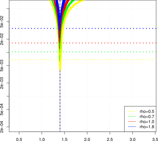
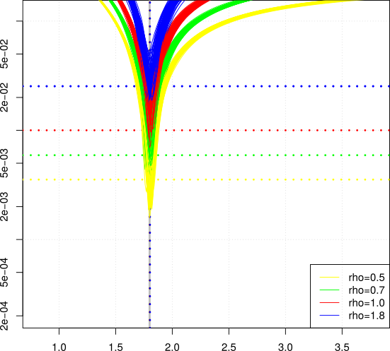
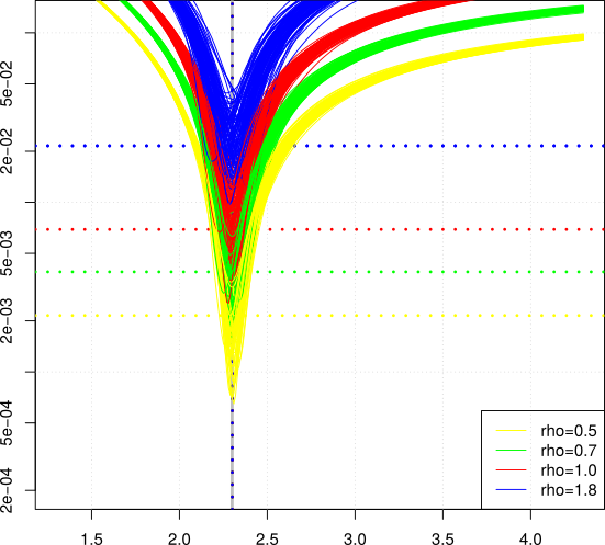
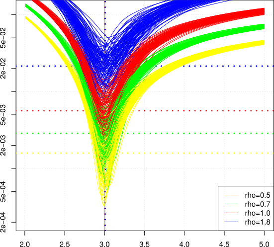
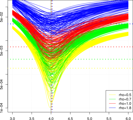
Figure 2: Plots (a) - (f) correspond to $\alpha_{0}\in\{0.7,1.4,1.8,2.3,3.0,4.0\}$, where on each plot you see four samples of $m=10$ curves with the cutoffs $\rho\in\{0.5,0.7,1.0,1.8\}$ which are color coded

$\longrightarrow$ Position of Figure 3

Figure 3: Simulation of the increments of a single realization of a compound Poisson process of intensity $1$ for tail index $\alpha_{0}=1.6$ and lower cutoff $\rho=0.5$ (left side) a compound Poisson process of intensity $1$ with standard normal $N(0,1)$ jump measure (right side).

$\longrightarrow$ Position of Figure 4

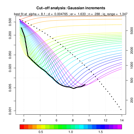
Figure 4: Cutoff sensitivity analysis for simulated data of a compound Poisson process of intensity $1$ with renormalized jump measure $\nu^{\alpha_{0}}$ with tail index $\alpha_{0}=1.6$ and lower cutoff $\rho=0.5$ (left side) and a compound Poisson process of intensity $1$ with standard normal $N(0,1)$ jump measure (right side). The number of points included for each colored curve is color coded as follows. If one picks a curve and detects its color (dark blue, say) and looks for the value of the black dashed line at the position of that (dark blue) color on the color spectrum one can read off on the right side the number of included points.

$\longrightarrow$ Position of Figure 5

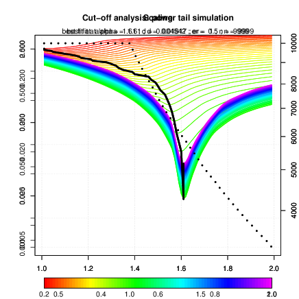
Figure 5: Scaling property of the coupling distance: Cutoff sensitivity analysis for simulated data of a compound Poisson process of intensity $1$ for with renormalized jump measure $\nu^{\alpha_{0}}$ with tail index $\alpha_{0}=1.6$. Here the data were multiplied with $2$, the lower cutoff is taken $\rho=2\times 0.5$ and the coupling distance cutoff $s=2^{2}$.

$\longrightarrow$ Position of Figure 6

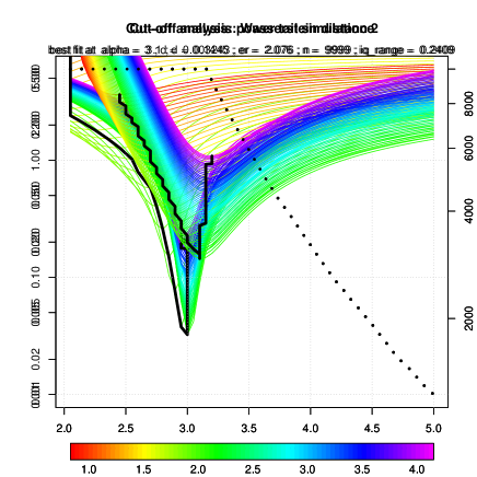
Figure 6: Cutoff sensitivity analysis for simulated data of a compound Poisson process of intensity $1$ with renormalized jump measure $\nu^{\alpha_{0}}$ with tail index $\alpha_{0}=1.6$ and lower cutoff $\rho=0.5$ (left side) and a compound Poisson process of intensity $1$ with standard normal $N(0,1)$ jump measure (right side)

5 Application to example climatic data sets

In this section we will apply the estimators discussed above to two sets of climatic data. Because the estimators as constructed assume stationary stochastic increments, that is essentially additive noise models with autonomous coefficients, the datasets we consider will be those for which the assumption of this increment stationarity is reasonable.

The first example which we discuss is a paleoclimatic time series of calcium concentration proxies (cf. [13]) which has received considerable interest in recent years. The second class of examples are data sets of precipitable water vapor from different measurement stations in the Western Tropical Pacific.

5.1 Paleoclimatic GRIP data

Paleoclimate proxy data from Greenland ice cores show clear evidence of two distinct states of high-latitude climate during the past glacial period (e.g. [29]). Residence time within both the relatively warm interstadial state and the relatively cool stadial state are in on order of $1000$ years (e.g. [10], [34]). Using the logarithm of the calcium concentration record (a measure of continental aridity which correlates well with proxy estimates of high-latitude temperature) from the Greenland Ice Core Project (GRIP), Ditlevsen [10] argued that the statistics of transitions between states shows evidence of $\alpha$-stable driving noise with $\alpha=1.75$.

$\longrightarrow$ Position of Figure 7

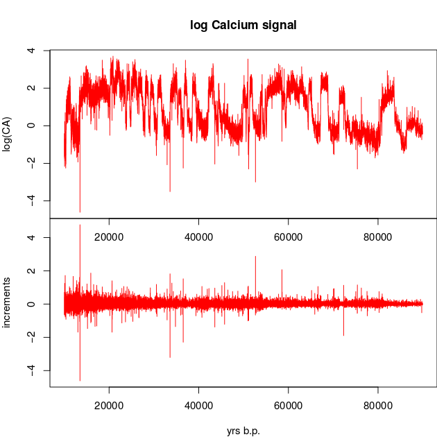
Figure 7: Paleoclimatic GRIP data

Motivated by the analysis in [10] there has been a series of works on the model selection problem ([15], [22], [21]), using different methods to estimate the tail index, which led to indications of $\alpha=0.75$ (that is following Section 2 an $\alpha$-stable process even without first moments) and $\alpha=1.75$ according with Ditlevsen’s proposal. These methods have been based on the self-similar scaling of $\alpha$-stable processes, which turns out to be a rather fragile property, since it enhances small errors to large scales.

In [18] we applied an earlier version of the estimation procedure described in this study to the same GRIP log calcium time series analyzed in [10]. Local best fits were obtained by tuning the parameters $\lambda$, $\rho$ and $\alpha$  for the positive tail at the cutoff $\rho^{+}=0.36$ and the index $\alpha_{0}^{+}=3.6$ and for the negative tail at $\rho^{-}=0.35$ and the index $\alpha_{0}^{-}=3.55$ with reasonable sample sizes $n^{+}=894$ and $n^{-}=530$ and small distances $d^{+}=0.081\ll 1$ and $d^{-}=0.089\ll 1$. A systematic optimization of the cutoff and the tails was not considered in this earlier study.

In this subsection we will re-analyze this time series using the procedure described in the second part of Subsection 4.2. First we standardize the tail intensity to $\lambda=1$. We then search for the pair $(\rho,\alpha_{0})$ such that the minimum of the curve $\alpha\mapsto\operatorname{\widetilde{\mathrm{w}_{n}}}(\alpha;\alpha_{0},\rho)(\omega)$ is minimal over all those parameter values.

$\longrightarrow$ Position of Figure 8

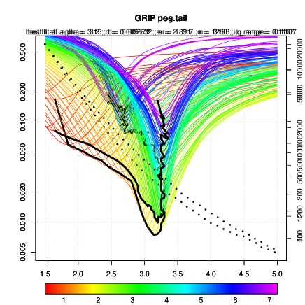
(a)

(b)

Figure 8: Plots of the functions $\alpha\mapsto\operatorname{\widetilde{\mathrm{w}_{n}}}(\alpha;\alpha_{0},\rho)(\omega)$ the negative and positive measure $\nu^{\alpha_{0}}$ for different parameters $\rho,\alpha_{0}$

The GRIP log calcium time series and that of its increments are shown in Figure 7. Both panels of Figure 8 show the functions $\alpha\mapsto\operatorname{\widetilde{\mathrm{w}_{n}}}(\alpha;\alpha_{0},\rho)(\omega)$ for different cutoffs $\rho$ ranging from $0.5$ (orange-red) to $7$ (pink). The left side of Figure 8 treats the negative tails of the empirical increment distributions and the right side the positive tails. For the negative tails the locus of minima yields a very distinctive minimum for a cutoff value of $\rho^{-}=1.71$ with approximately $n=3186$ data points and with a minimal distance at $d^{-}=0.00732$ and the best fit for the tail index $\alpha^{-}\approx 3.15$. The minimal distance is of the magnitude of the simulated compound Poisson data of Figure 4(left side) and indicates a clear polynomial behavior. For the positive tails this picture is even more pronounced with an even sharper minimum for approximately the same cutoff value $\rho^{+}\approx 3.2$ with approximately $n=1260$ data points and minimal distance of $d^{+}=0.00987$ and estimated tail index $\alpha^{+}=3.2$. For larger values of the cutoff, the curve of minima moves upward rather than laterally until the number of data points entering the analysis becomes very small. This relative insensitivity of the estimated tail index to the cutoff values is further evidence of polynomial tails in the driving noise.

The results of this analysis provide strong evidence for polynomial tails in the driving process in these data, consistent with the results of [22], [15], [14].

However, consistent with our earlier estimates in [18], we find that the tail parameter $\alpha$ is greater than two, so the increment distribution of the driving noise process has finite variance. The detection of tail behaviour with $\alpha>2$ in these data is noteworthy. Classical homogenization or stochastic averaging results such as [30] indicate that for coupled dynamics in which a slow variable is driven by a finite variance fast variable, the asymptotic dynamics in the limit of infinite scale separation should be a standard stochastic differential equation with Brownian noise. The presence of driving noise with finite-variance, polynomial-tailed increments in the GRIP data is suggestive that the timescale separation between fast and slow processes is not sufficiently large in this setting for the asymptotic dynamics to hold.

5.2 Western Tropical Pacific precipitable water vapor data

The second observational data we consider are two time series of hourly-mean precipitable water vapor (PWV, the total water content of the atmospheric column, in cm) from the islands Nauru ($0.5^{\circ}$ S, $166.9^{\circ}$ E) and Manus ($2.1^{\circ}$ S, $147.4^{\circ}$ E) in the Western Tropical Pacific. The Nauru PWV time series extends from January 1 1998 to December 31 2010, and the Manus time series from January 1 1996 to December 31 2011. These data were obtained from the ARM (Atmospheric Radiation Measurement) Best Estimate Data set ([41]), and downloaded from www.archive.arm.gov.

These data were investigated because the onset of convective precipitation is a threshold process that occurs when at least part of the atmospheric column becomes saturated with regards to water vapor. While in the non-precipitating state PWV can be considered to undergo gradual random variations, the transition to the precipitating state produces a rapid decrease in column water content. Recent analysis [32] has shown that the probability distribution of rainfall event magnitudes has a power-law tail, as do dry spell duration and (to a lesser extent) precipitation event duration. Furthermore, [36] and [37] have demonstrated that a simple two-state precipitation on and off stochastic differential equation model for column moisture can reproduce the observed statistics of precipitation. The jump-like changes in PWV resulting from the rapid onset of precipitation suggest that on sufficiently coarse timescales the driving process of PWV could be represented as an alpha-stable process (for at least the negative increments).

$\longrightarrow$ Position of Figure 9

(a)

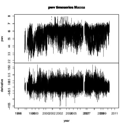
(b)

Figure 9: $16$ years of precipitable water vapor data of the measurement station on Manus island and the respective data increments (a), the same for Nauru island (b) .

$\longrightarrow$ Position of Figure 10

(a)

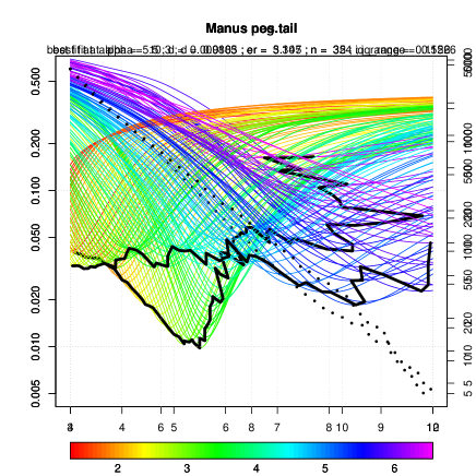
(b)

(c)

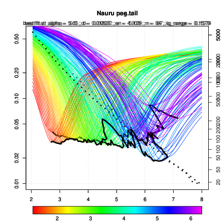
(d)

Figure 10: Plots of the functions $\alpha\mapsto\operatorname{\widetilde{\mathrm{w}_{n}}}(\alpha;\alpha_{0},\rho)(\omega)$ the negative and positive measure $\nu^{\alpha_{0}}$ for different parameters $\rho,\alpha_{0}$ of the Manus island data (a) and (b) and Nauru island (c) and (d)

Time series of PWV and its increments from Manus and Nauru are shown in Figure 9. Unlike the time series at Manus, that at Nauru shows evidence of low frequency variations (in the local mean for PWV and in the amplitude of fluctuations for the increments). Plots of the functions $\alpha\mapsto\operatorname{\widetilde{\mathrm{w}_{n}}}(\alpha;\alpha_{0},\rho)(\omega)$ for the positive and negative tails of the increments distributions for both locations are shown in Figure 10. For the negative tail at Manus, the locus of curve minima over individual cut-offs $\rho$ takes a clear minimum at $\alpha_{0}=5.5$ (corresponding to a cut-off of $\rho=3.2$ and $\sim$150 data points), beyond which it rises with increasing $\rho$. The lateral meandering for $\rho\gtrsim 5$ is interpreted as resulting from the small number of data points entering the computation. In contrast, the locus of curve minima for the positive tail at Manus shows no evidence of a robust global minimum value. Similar results are found at Nauru. The locus of curve minima for the negative tail shows a global minimum at $\alpha_{0}=6.5$ ($\rho\simeq 4.5$, $\sim 100$ data points), beyond which it increases. No evidence of a minimum is seen for the positive tail. The global minimum of the locus of curve minima for the negative tail is not as pronounced as at Manus, perhaps because of the low-frequency variability present in the PWV time series at Nauru. These results show strong evidence of polynomial behavior in the negative tail of PWV, consistent with the effects of episodic drying of the water column by convective precipitation events. No such threshold process produces jumps increasing PWV, and correspondingly no evidence is found of polynomial tails for the positive increments. The difference in the values of $\alpha_{0}$ obtained for negative increments at the two locations (5.5 at Manus and 6.5 at Nauru) could reflect real differences in moist processes at the two stations or could simply be a result of sampling variability due to the relatively short time series. The observed universality of precipitation event size distributions in [32] suggests that sampling variability is likely a large contributor to this difference. Finally, as with the ice core data considered above, the detection of polynomial tails in the PWV driving process with $\alpha_{0}>2$ indicates that the separation between fast and slow timescales in PWV dynamics is not sufficiently large for the central limit theorem to render this driving process effectively Gaussian.

6 Conclusion

This study presents a new method in time series analysis for the assessment of the proximity of data to power-law Lévy diffusions. Our method is based on the notion of coupling distance recently introduced in the mathematics literature in order to measure the distance between such models on path space (Theorems 2.2 and 2.1). The underlying statistical analysis involves a modification of the empirical Wasserstein distance, which is easily implementable and has favorable properties such as good asymptotic convergence rates as we have confirmed by extensive simulation studies for different data lengths, tail exponents and cutoff thresholds. In particular, this statistic is consistent with the Wasserstein distance, whenever the latter exists.

We stress that while this method provides insight into the noise structure of the large increments in the underlying data even on a pathwise level, it does not resconstruct the deterministic forcing $f$. For this purpose other methods analyzing the small data increments have to be applied. The construction of confidence intervals for the tail exponent is subject to future research. It is also remarkable that this method worked out in detail for the one-parameter family of power-law tail exponents can be adapted to other one-parameter families of Lévy measures.

The coupling distance curves introduced in this study provide a device for intuitive visual inspection in order to detect a power-law behavior of the driving jump noise. It is also shown how the characteristic structures of Gaussian and power-law processes are clearly distinguishable. In particular, this approach allows the detection of the presence of $\alpha$-stable signals, where the Wasserstein distance is not defined.

The central statistical estimate of our method compares the empirical quantile function of the truncated increments of the time series to the quantile function of the candidate process being tested. While other more intuitive approaches to this comparison (such as curve fitting using the empirical histogram of increments) may be simpler, our approach has the benefit of being rigorous, providing rate of convergence results, and of generalizing in a straightforward way to a broad class of stochastic differential equations (e.g. multiplicative or non-autonomous noise coefficients), driving processes (e.g. not necessarily alpha-stable) and parameters of interest (e.g. a skewness parameter instead of the tail exponent).

The concept of coupling distance curves relies heavily on the knowledge of the explicit minimizer of the Wasserstein distance in one dimension. In higher dimensions, however, the optimal coupling is not known in closed form. Therefore any coupling will only provide upper bounds. Furthermore, it is worth noting that coupling distances were developed for models with additive noise (see the modeling assumptions in Section 3.3). To treat more general stochastic differential equation models with multiplicative noise dependence the notion of transportation distance has been introduced [19]. Its statistical implementation is subject to further study.

Our method was finally applied to an often-studied set of paleoclimate data and confirms our previous results in [18], where the tail exponents were determined by a non-systematic application of coupling distances. In addition, we systematically analyze a set of atmospheric data from the Western Tropical Pacific and detected polynomial tail exponents interpreted as resulting from the threshold behavior of precipitation. Future studies will generalize the approach considered in this study to allow analysis of time series with strong deterministic non-stationarities such as annual or diurnal cycles.

References

- [1] D. Applebaum. Lévy processes and stochastic calculus. Cambridge university press, 2009.
- [2] E. del Barrio, P. Deheuvels, S. van de Geer. Lectures on Empirical Processes. Series of Lectures in Mathematics of the EMS, 2007.
- [3] R. Benzi, G. Parisi, A. Sutera, A. Vulpiani. Stochastic resonance in climate change. Tellus, 34:10-16, 1982.
- [4] N. Berglund, D. Landon. Mixed-mode oscillations and interspike interval statistics in the stochastic FitzHugh-Nagumo model. Nonlinearity, 25:2303-2335, 2012.
- [5] N. Berglund, B. Gentz. Metastability in simple climate models: Pathwise analysis of slowly driven Langevin equations. Stoch. Dyn., 2:327-356, 2002.
- [6] P. Billingsley. Convergence of probability measures. Wiley series in probability and statistics, 1999.
- [7] N. H. Bingham, C. M. Goldie, J. L. Teugels. Regular variation. Cambridge University Press, 1987.
- [8] M. Csörgö, C. Horváth, On the distributions of Lp norms and weighted uniform empirical and quantile processes. The Annals of Probability, (16) (1) 142–161, 1988.
- [9] M. Csörgö, C. Horváth, On the distributions of Lp norms and weighted quantile processes. Annales de l’I.H.P., section B (26) (1) 65–85, 1990.
- [10] P.D. Ditlevsen. Observation of a stable noise induced millennial climate changes from an ice-core record. Geophysical Research Letters, 26 (10):1441–1444, 1999.
- [11] C. Doss, M. Thieullen. Oscillations and random perturbations of a FitzHugh-Nagumo system. Preprint hal-00395284, 2009.
- [12] W. Feller. An introduction to probability theory and its applications. Vol. II, John Wiley & Sons, 1971.
- [13] K. Fuhrer, A. Neftel, M. Anklin, V. Maggi. Continuous measurement of hydrogen-peroxide, formaldehyde, calcium and ammonium concentrations along the new GRIP Ice Core from Summit, Central Greenland. Atmos. Environ. Sect. A, 27, 1873-1880, 1993.
- [14] J. Gairing. Speed of convergence of discrete power variations of jump diffusions. Diplom thesis, Humboldt-Universität zu Berlin, 2011
- [15] J. Gairing, P. Imkeller. Stable CLTs and rates for power variation of -stable Lévy processes. Methodology and Computing in Applied Probability, 1-18, 2013.
- [16] A. Debussche, M. Högele, P. Imkeller. The dynamics of non-linear reaction-diffusion equations with small Lévy noise. Springer Lecture Notes in Mathematics, Vol. 2085, 2013.
- [17] J. Gairing, M. Högele, T. Kosenkova, A. Kulik. Coupling distances between Lévy measures and applications to noise sensitivity of SDE. Stochastics and Dynamics, 15 (2), 1550009-1 – 1550009-25 (2014), DOI:10.1142/S0219493715500094
- [18] J. Gairing, M. Högele, T. Kosenkova, A. Kulik. On the calibration of Lévy driven time series with coupling distances with an application in paleoclimate. in Springer-INdAM Series, vol. 15, “Mathematical Paradigms of Climate Sciences” (2016), Springer, Milan, Heidelberg, ISBN 978-3-319-39091-8
- [19] J. Gairing, M. Högele, T. Kosenkova. Transportation distances and noise sensitivity of multipicative Lévy SDE with applications. https://arxiv.org/abs/1511.07666
- [20] K. Hasselmann. Stochastic climate models: Part I. Theory. Tellus, 28:473–485, 1976.
- [21] C. Hein, P. Imkeller, I. Pavlyukevich. Limit theorems for p-variations of solutions of SDEs driven by additive stable Lévy noise and model selection for paleo-climatic data. Interdisciplinary Math. Sciences, 8:137-150, 2009.
- [22] C. Hein, P. Imkeller, I. Pavlyukevich. Simple SDE dynamical models interpreting climate data and their meta-stability. Oberwolfach Reports, 2008
- [23] M. Högele, I. Pavlyukevich. The exit problem from the neighborhood of a global attractor for heavy-tailed Lévy diffusions. Stochastic Analysis and Applications, 32 (1), 163–190 (2013)
- [24] P. Imkeller, A. Monahan. Conceptual stochastic climate models. Stochastics and Dynamics, 2:311–326, 2002.
- [25] P. Imkeller. Energy balance models: Viewed from stochastic dynamics. Prog. Prob., 49:213–240, 2001.
- [26] P. Imkeller and I. Pavlyukevich. First exit times of SDEs driven by stable Lévy processes. Stochastic Processes and their Applications, 116(4):611–642, 2006.
- [27] P. Imkeller, I. Pavlyukevich, T. Wetzel. First exit times for Lévy-driven diffusions with exponentially light jumps. Ann. Probab., 37 (2) 530-564, 2009.
- [28] Members NGRIP. NGRRIP data. Nature, 431:147–151, 2004.
- [29] A. H. Monahan, J. Alexander, A. J. Weaver Stochastic models of meridional overturning circulation: time scales and patterns of variablility. Phil. Trans. R. Soc. A, 366: 2527-2544, 2008.
- [30] G. C. Papanicolau, W. Kohler. Asymptotic theory of mixing stochastic ordinary differential equations. Communications on Pure and Applied Mathematics, Vol. XXVII, 641-668, 1974.
- [31] I. Pavlyukevich. First exit times of solutions of stochastic differential equations with heavy tails. Stochastics and Dynamics, 11, Exp.No.2/3:1–25, 2011.
- [32] Peters, O. A. Deluca, A. Corral, J. D. Neelin, C. E. Holloway. Universality of rain event size distributions. J. Stat. Mech: Theory and Experiment. 2010. doi:10.1088/1742-5468/2010/11/P11030
- [33] S. T. Rachev, L. Rüschendorf. Mass Transportation Problems. Vol.I: Theory, Vol.II.: Applications. Probability and its Applications. Springer-Verlag, New York 1998.
- [34] S. Rahmstorf. Timing of abrupt climate change: a precise clock. Geophys. Res. Let.. 30, 1510, 2003.
- [35] K. Sato. Lévy processes and infinitely divisible distributions, volume 68 of Cambridge Studies in Advanced Mathematics. Cambridge University Press, 1999.
- [36] S. N. Stechmann, J. D. Neelin. A stochastic model for the transition to strong convection. J. Atmos. Sci. 68, 2955-2970, 2011.
- [37] S. N. Stechmann, J. D. Neelin. First-passage-time prototypes for precipitation statistics. J. Atmos. Sci. 71, 3269-3291, 2014.
- [38] G. Samoradnitsky, M. Taqqu. Stable non-Gaussian random processes. Chapman& Hall. Boca-Raton, London, New York, Washington D.C. 1994.
- [39] H.C. Tuckwell, R. Rodriguez, F.Y.M. Wan, Determination of firing times for the stochastic Fitzhugh-Nagumo neuronal model. Neural Computation, 15:143 – 159, 2003.
- [40] A.W. van der Vaard, J.A.Wellner, Weak convergence and empirical processes. Springer Series in Statistics, 1996.
- [41] S. Xie and coauthors, ARM Climate Modelling Best Estimate Data: A New Data Product for Climate Studies. Bull. Amer. Meteo. Soc. , 91, 13-20, 2010.