The O₂ A–band in fluxes and polarization of starlight
reflected by Earth–like exoplanets

Abstract

Earth–like, potentially habitable exoplanets are prime targets in the search for extraterrestrial life. Information about their atmosphere and surface can be derived by analyzing light of the parent star reflected by the planet. We investigate the influence of the surface albedo $A_{\rm s}$, the optical thickness $b_{\rm cloud}$ and altitude of water clouds, and the mixing ratio of biosignature O₂ on the strength of the O₂ A–band (around 760 nm) in flux and polarization spectra of starlight reflected by Earth–like exoplanets. Our computations for horizontally homogeneous planets show that small mixing ratios ($\eta<0.4$) will yield moderately deep bands in flux and moderate to small band strengths in polarization, and that clouds will usually decrease the band depth in flux and the band strength in polarization. However, cloud influence will be strongly dependent on their properties such as optical thickness, top altitude, particle phase, coverage fraction, horizontal distribution. Depending on the surface albedo, and cloud properties, different O₂ mixing ratios $\eta$ can give similar absorption band depths in flux and band strengths in polarization, in particular if the clouds have moderate to high optical thicknesses. Measuring both the flux and the polarization is essential to reduce the degeneracies, although it will not solve them, in particular not for horizontally inhomogeneous planets. Observations at a wide range of phase angles and with a high temporal resolution could help to derive cloud properties and, once those are known, the mixing ratio of O₂ or any other absorbing gas.

1 Introduction

After more than two decades of exoplanet detections, statistics shows that, on average, every star in the Milky Way has a planet, and that at least 20$\%$ of the solar–type stars have a rocky planet in their habitable zone (Petigura et al., 2013), the region around a star where planets receive the right amount of energy to allow water to be liquid on their surface (see, e.g. Kasting et al., 1993) (assuming they have a solid surface). Recently, Proxima Centauri, the star closest to our Sun, was shown to host a potentially rocky planet in its habitable zone (Anglada-Escudé et al., 2016). Planets in habitable zones are prime targets in the search for extraterrestrial life because liquid water is essential for life as we know it. Whether or not a rocky planet has liquid surface water also depends on the thickness, composition and structure of its atmosphere. Narrowing down planets in our search for extraterrestrial life thus requires the characterisation of planetary atmospheres in terms of composition and structure, as well as surface pressure and albedo. Of particular interest is the search for biosignatures, i.e. traces of present or past life, such as the atmospheric gases oxygen and methane, and for habitability markers, such as liquid surface water.

Gases like oxygen and methane are too chemically reactive to remain in significant amounts in any planetary atmosphere without continuous replenishment. The current globally averaged mixing ratio of biosignature (and greenhouse gas) methane is much smaller than that of dioxygen, i.e. only about 1.7 $\cdot~{}10^{-6}$. Also due to its distinct sources, its distribution varies both horizontally and vertically across the Earth and in time. The dioxygen mixing ratio in the current Earth’s atmosphere is about 0.21 and virtually altitude–independent. Although oxygenic photosynthetic organisms appeared about 3.5 $\cdot~{}10^{9}$ years ago, the oxygen they produced was efficiently chemically removed from the atmosphere by combining with dissolved iron in the oceans to form banded iron formations (Crowe et al., 2013). It is thought that when this oxygen sink became saturated, the atmospheric free oxygen started to increase in the so–called Great Oxygenation Event (GOE) around 2.3 $\cdot~{}10^{9}$ years ago. While after the GOE, the oxygen mixing ratio remained fairly low and constant at about 0.03 for about 10⁹ years, it started to rise rapidly about 10⁹ years ago to maximum levels of 0.35 about 2.80 $\cdot~{}10^{8}$ years ago. Since then, the ratio has leveled off to its current value (Crowe et al., 2013). The triatomic form of oxygen, ozone, is formed by photodissociation of dioxygen molecules. Ozone protects the Earth’s biosphere from harmful UV–radiation by absorbing it. The ozone mixing ratio is variable and shows a prominent peak between about 20 and 30 km of altitude, the so–called ozone–layer.

In this paper, we investigate the planetary properties that determine the appearance of gaseous absorption bands in spectra of starlight reflected by exoplanets with Earth–like atmospheres. We concentrate on the so–called O₂ A–band, centered around 760 nm, the strongest absorption band of O₂ across the visible. The advantage of concentrating on this band is not only that it appears to be a strong biosignature, but also that the range of absorption optical thicknesses across the band is large and thus probes virtually all altitudes within an atmosphere (assuming it is well–mixed throughout the atmosphere). The identification of biosignatures like oxygen and methane in an exoplanet signal will depend on the presence of the spectral features they leave in a planetary spectrum. The retrieval of the mixing ratio of an atmospheric gas will rely on the strength on the spectral features. This strength with respect to the continuum surrounding a feature will depend on the intrinsic strength of the feature, i.e. the absorption cross–section of the molecules and their atmospheric column number density (in molecules m^-2). It will also be affected by clouds in the atmosphere, as they will cover (part) of the absorbing molecules, and as they will change the optical path lengths of the incoming photons and hence change the amount of absorption (Fujii et al., 2013). The precise influence of clouds will depend on the (horizontal and vertical) distribution of the absorbing gases and on the cloud properties: their horizontal and vertical extent, cloud particle column number densities, the cloud particle microphysical properties, such as particle size distribution, composition, and even shape. Through the cloud particle microphysical properties, the influence of clouds on spectral features of atmospheric gases will thus also depend on the wavelength region under consideration.

On Earth, the O₂ mixing ratio is known and constant up to high altitudes. Therefore, as postulated by Yamamoto & Wark (1961) and demonstrated by Fischer & Grassl (1991) and Fischer et al. (1991), the depth of the O₂ A–band in spectra of sunlight reflected by a region of the Earth that is covered by an optically thick cloud layer allows to estimate cloud top altitudes. Because of the strength of the O₂ A–band, this method is sensitive to both high and low clouds and appears to be insensitive to temperature inversions. The method is widely applied both to measurements taken from airplanes (e.g. Lindstrot et al., 2006) and to satellite data (see Saiedy et al., 1965; Vanbauce et al., 1998; Koelemeijer et al., 2001; Preusker et al., 2007; Lelli et al., 2012; Desmons et al., 2013). However, because this method only accounts approximately for the penetration and multiple scattering of photons inside the cloud, it tends to systematically overestimate cloud top pressures (hence it underestimates cloud top altitudes) (Vanbauce et al., 1998). The retrieved pressure appears to be more representative to the pressure halfway the cloud (see Vanbauce et al., 2003; Wang et al., 2008; Sneep et al., 2008; Ferlay et al., 2010; Desmons et al., 2013).

In Earth remote–sensing, the retrieval of cloud top altitudes is important for climate research and especially for the retrieval of atmospheric column densities of trace gases, such as ozone and methane, that will be partly hidden from the view of Earth–orbiting satellites when clouds are present. Not surprisingly, there is little interest in deriving O₂ mixing ratios.

In exoplanet research, however, the O₂ mixing ratio will be unknown, and absorption band depths cannot be used to derive cloud top altitudes. Indeed, the direct detection of exoplanetary radiation to investigate the depth of gaseous absorption bands is extremely challenging, because of the huge flux contrast between a parent star and an exoplanet and the small angular separation between the two. Konopacky et al. (2013) were the first to succeed in capturing a thermal spectrum of one of the exoplanets around the star HR 8799 through spatially separating it from its star. The spectrum of this young and hot, and thus thermally bright, planet shows molecular lines from water and carbon monoxide. Because of their moderate temperatures, potentially habitable exoplanets will not be very luminous at infrared wavelengths and the relatively small size of rocky exoplanets will require highly optimized telescopes and instruments for their characterization. Examples of current instruments that aim at spatially resolving large, gaseous, old and cold exoplanets from their parent star and characterizing them from their directly detected signals are SPHERE (Spectro-Polarimetric High-contrast Exoplanet Research) (see Beuzit et al., 2006, and references therein) on ESO’s Very Large Telescope (VLT), GPI (Gemini Planet Finder) (see Macintosh et al., 2014) on the Gemini North telescope, CHARIS (Coronographic High Angular Resolution Imaging Spectrograph) (see Groff et al., 2014) on the Subaru telescope, and HROS (High–Resolution Optical Spectrograph) for the future TMT (Thirty Meter Telescope) (Froning et al., 2006; Osterman et al., 2006). The future European Extremely Large Telescope (E–ELT) also has the characterization of Earth–like exoplanets as one of its main science cases.

Both SPHERE and GPI can measure not only thermal fluxes that their target planets emit and fluxes of starlight that the planets reflect, but they can also measure the state of polarization of the planetary radiation. In particular, SPHERE has a polarimetric optical arm that is based on the ZIMPOL (Zürich Imaging Polarimeter) technique (Schmid et al., 2005; Gisler et al., 2004) (IRDIS, an infrared arm of SPHERE, has polarimetric capabilities designed for observations of circumstelllar matter, but potentially of use for exoplanet detection, too). Polarimetry is also a technique that will be used in EPICS, the Earth–like Planet Imaging Camera System (Gratton et al., 2011; Keller et al., 2010), that is being planned for the E–ELT. First detections of polarimetric signals of exoplanets have been claimed (see Wiktorowicz et al., 2015; Bott et al., 2016, and references therein).

There are several advantages of using polarimetry in exoplanet research. Firstly, light of a solar–type star can be assumed unpolarized (see Kemp et al., 1987) when integrated across the stellar disk, while starlight that has been reflected by a planet will usually be (linearly) polarized (see e.g. Seager et al., 2000; Stam et al., 2004; Stam, 2008). Polarimetry can thus increase the much–needed contrast between a planet and its parent star (Keller, 2006) and facilitate the direct detection of an exoplanet. Secondly, detecting a polarized object in the vicinity of a star would immediately confirm the planetary nature of the object, as stars or other background objects will have a negligible to low degree of polarization. Thirdly, the state of polarization of the starlight (in particular as functions of the planetary phase angle and/or wavelength) that has been reflected by the planet is sensitive to the structure and composition of the planetary atmosphere and surface, and could thus be used for characterizing the planet, e.g. by detecting clouds and hazes and their composition. A famous example of this application of polarimetry is the derivation of the size and composition of the cloud droplets that form the ubiquitous Venus clouds from disk–integrated polarimetry of reflected sunlight at three wavelengths and across a broad phase angle range by Hansen & Hovenier (1974) (thus similar observations as would be available for direct exoplanet observations, with the exoplanet’s phase angle range depending on the orbital inclination angle). These cloud particle properties, that were later confirmed by in–situ measurements, could not be derived from the spectral and phase angle dependence of the sunlight’s reflected flux, because flux phase functions are generally less sensitive to the microphysical properties of the scattering particles. For exoplanets, Karalidi et al. (2012) and Bailey (2007) have numerically shown that the primary rainbow of starlight that has been scattered by liquid water cloud particles on a planet should be observable for relatively small water cloud coverage ($10\%-20\%$), even when the liquid water clouds are partly covered by ice water clouds (which themselves do not show the rainbow feature). In Earth–observation, the PARASOL/POLDER instrument–series (Fougnie et al., 2007; Deschamps et al., 1994) uses polarimetry to determine the phase of the (water) clouds it observes (see e.g. Goloub et al., 2000).

In this paper, we not only investigate influences on the O₂ A–band in flux spectra of starlight that is reflected by exoplanets, but also in polarization spectra. Indeed, gaseous absorption bands not only show up in flux spectra of light reflected by (exo)planets, they usually also appear in polarization spectra (see Boesche et al., 2008; Joos & Schmid, 2007; Stam et al., 2004; Aben et al., 2001; Stam et al., 1999, for examples in the Solar System).

There are two main reasons why absorption bands appear in polarization spectra, despite polarization being a relative measure, i.e. the polarized flux divided by the total flux. Firstly, with increasing absorption, the reflected light contains less multiple scattered light, which usually has a lower polarization than the singly scattered light. The relative increase of the contribution of singly scattered light to the reflected signal thus increases its degree of polarization. Secondly, with increasing absorption, the altitude at which most of the reflected light has been scattered increases. If different altitude regions of the atmosphere contain different types of particles, with different single scattering polarization signatures, the polarization will vary across an absorption line, with the degree of polarization in the deepest part of the line representative for the particles in the higher atmospheric layers, and the polarization in the continuum representative for the particles in the lower, usually denser atmospheric layers. For an in–depth explanation of these effects, see Stam et al. (1999). Note that while attenuation through the Earth’s atmosphere will change the flux of an exoplanets, it does not change the degree of polarization across gaseous absorption bands in a spectrum of a planet or exoplanet. This is an additional advantage of using polarimetry for the detection of gaseous absorption bands with ground–based telescopes, in particular when (exo)planet observations are pursued in wavelength regions where the Earth’s atmosphere itself absorbs light.

The results presented in this paper can not only be used to investigate the retrieval of trace gases and cloud properties of exoplanets. They will also be useful for the design and optimization of spectrometers for exoplanetary detection and characterization: the optical response of mirrors, lenses, and e.g. gratings usually depends on the degree and direction of the light that is incident on them, and when observing a polarized signal, such as starlight that has been reflected by an exoplanet, the detected flux signal will depend on the degree and direction of polarization of the incoming light. In particular, the detected depth of a gaseous absorption band, and hence the gaseous mixing ratio that will be derived from it, thus depends on the polarization across the band. Even if a telescope’s and/or instrument’s polarization sensitivities are fully known, detected fluxes can only be accurately corrected for polarization sensitivities if the polarization of the observed light is measured as well (see Stam et al. , 2000, for examples of such corrections). In the absence of such polarization measurements, numerical simulations such as those presented in this paper can help to assess the uncertainties.

The structure of this paper is as follows. In Sect. 2, we describe our method for calculating the flux and polarization of starlight that is reflected by an exoplanet, including our disk–integration technique and how we handle the spectral computations. In Sect. 3, we present our numerical results for cloud–free, completely cloudy and partly cloudy exoplanets. Finally, in Sects. 4 and 5, we discuss and summarize our results.

2 Calculating reflected starlight

2.1 Flux vectors and polarization

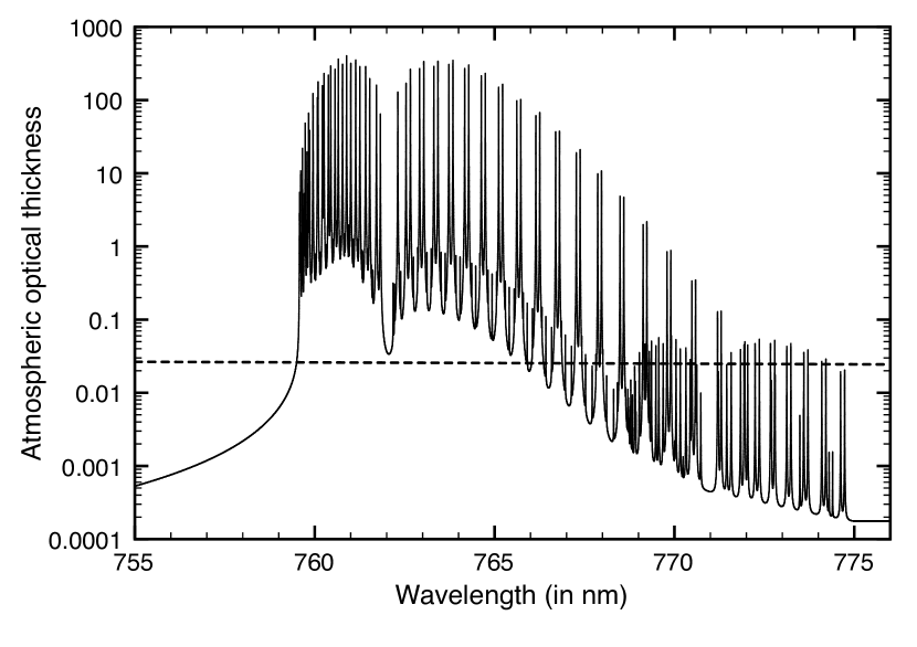
Figure 1: Solid line: the gaseous absorption optical thickness of the Earth’s atmosphere across the O₂ A–band, computed for a model atmosphere, using a mid–latitude summer pressure–temperature profile (McClatchey et al. , 1972) and absorption line parameters from Rothman et al. (2005). Dashed line: the computed gaseous scattering optical thickness of the same model atmosphere. Its value decreases from 0.027 at 755 nm to 0.024 at 775 nm. Details on the used absorption line profiles and computation can be found in Stam et al. (2000).

The flux and state of polarization of starlight that is reflected by a spatially unresolved exoplanet and that is received by a distant observer, is fully described by a flux (column) vector, as follows

$$\pi{\bf F}=\pi\left[F,Q,U,V\right],$$ (1)

with $\pi F$ the total flux, $\pi Q$ and $\pi U$ the linearly polarized fluxes, defined with respect to a reference plane, and $\pi V$ the circularly polarized flux (for details on these parameters, see e.g. Hovenier et al., 2004; Hansen & Travis, 1974). We use the planetary scattering plane, i.e. the plane through the centers of the planet, the star and the observer, as the reference plane for parameters $Q$ and $U$.

Integrated over the stellar disk, light of a solar–type star can be assumed to be virtually unpolarized (Kemp et al., 1987). We thus describe its flux vector as ${\bf\pi F_{0}}=\pi F_{0}\left[1,0,0,0\right]=\pi F_{0}{\bf 1}$, with $\pi F_{0}$ the stellar flux measured perpendicular to the direction of propagation of the light, and ${\bf 1}$ the unit (column) vector.

Integrated over the illuminated and visible part of a planetary disk, the starlight that is reflected by a planet will usually be linearly polarized with the degree of polarization depending on the properties of the planetary atmosphere and surface (if present) (see, e.g. Stam, 2008; Stam et al., 2006, 2004). The reflected starlight can also be partly circularly polarized, because our model atmospheres contain not only Rayleigh scattering gases but also cloud particles (see Sect. 2.2). While Rayleigh scattering alone doesn’t circularly polarize light, light that has been scattered once and is linearly polarized, can get circularly polarized when it is scattered by cloud particles. The circularly polarized flux $V$ of a planet is usually very small (see Kemp , 1971; Hansen & Travis, 1974; Kawata, 1978), in particular when integrated over the planetary disk (Rossi et al. , 2017, in preparation). In the following, we therefore neglect $V$. This doesn’t introduce significant errors in $F$, $Q$, and $U$ (see Stam & Hovenier, 2005).

We define the degree of linear polarization of the reflected light as

$$P=\frac{\sqrt{Q^{2}+U^{2}}}{F},$$ (2)

which is independent of the choice of reference plane. In case $U=0$, which is true for planets that are mirror–symmetric with respect to the reference plane, the direction of polarization can be included into the definition of the degree of polarization:

$$P_{\rm s}=-Q/F$$ (3)

If $U=0$ and $Q<0$, the light is polarized parallel to the reference plane and $P_{\rm s}\geq 0$, while if $U=0$ and $Q\geq 0$, the light is polarized perpendicular to the reference plane and $P_{\rm s}<0$.

2.2 The planetary model atmospheres and surfaces

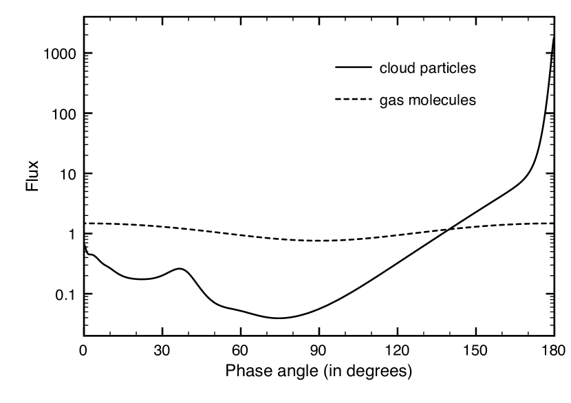
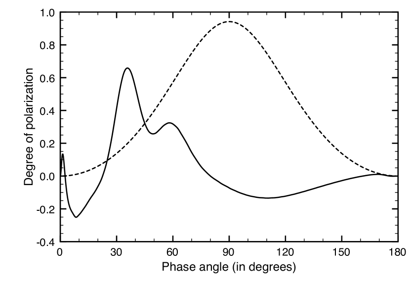
Figure 2: The total flux (left) and degree of linear polarization (right) of unpolarized incident light at $\lambda=765$ nm, that is singly scattered by samples of the cloud particles (solid lines) and samples of the Rayleigh scattering gas molecules (dashed lines) as functions of the phase angle (i.e. 180^∘ - the single scattering angle). The flux and polarization peak around 35^∘ in the cloud particle curves is the primary rainbow.

The atmospheres of our model planets are composed of stacks of locally horizontally homogeneous layers, containing gas molecules and, optionally, cloud particles. We assume the gas is terrestrial air and use pressure–temperature profiles representative for the Earth (McClatchey et al. , 1972).

For our model planets, we calculate $b_{\rm abs}$, the gaseous absorption optical thickness of the atmosphere, as the integral of the mixing ratio $\eta$ of the absorbing molecules times the gaseous number density (in m^-2) times the absorption cross–section $\sigma_{\rm abs}$ (in m²) along the vertical direction. Both $\eta$ and $\sigma_{\rm abs}$ usually depend on the ambient pressure and temperature, and thus on the altitude. Figure 1 shows the computed $b_{\rm abs}$ of the Earth’s atmosphere across the wavelength region with the $O_{2}$ A–band, with a spectral resolution high enough to resolve individual absorption lines. We have calculated this $b_{\rm abs}$ following Stam et al. (2000), assuming that $O_{2}$ is well–mixed, with $\eta=0.21$. Note that $b_{\rm sca}$, the gaseous scattering optical thickness of the Earth’s atmosphere is about 0.0255 in the middle of the absorption band.

Figure 2 shows the flux and degree of linear polarization of unpolarized incident light that is singly scattered by a sample of gas molecules. Here, we used the Rayleigh scattering matrix described by Hansen & Travis (1974) with a depolarization factor of 0.03. The depolarization factor modifies the isotropic Rayleigh scattering matrix (that applies to molecules that are perfect dipoles) to that of most molecules found in planetary atmospheres, whose scattering exhibits some anisotropy (for details, see Young , 1981). Although Fig. 2 pertains to singly scattered light, we use the phase angle (i.e. $180-\Theta$, with $\Theta$ the single scattering angle) to facilitate the comparison with planetary light curves later on.

The cloud particles are spherical and consist of liquid water with a refractive index of 1.335. The cloud particles are distributed in size according to a log–normal size distribution (see Eq. 2.56 in Hansen & Travis, 1974), with an effective radius of 6.0 $\mu$m and an effective variance of 0.5. We calculate the single scattering properties of the cloud particles using Mie–theory and the algorithm described by de Rooij & van der Stap (1984). Figure 2 shows the flux and degree of linear polarization of unpolarized incident light that is singly scattered by a sample of the cloud particles at $\lambda=765$ nm. Because we only consider the  20 nm wide wavelength region of the O₂ A–band, we ignore any wavelength dependence of the single scattering properties of cloud particles.

The surface below the atmospheres is locally horizontally homogeneous and reflects Lambertian, i.e. isotropic and unpolarized, with a surface albedo $A_{\rm s}$. While our model atmospheres and surfaces are locally horizontally homogeneous, our model exoplanets can be globally horizontally inhomogeneous, for example, they can be covered by patchy clouds (see Sect. 3.3).

2.3 Integration across the planetary disk

We perform the calculations of the starlight that is reflected by a spherical model planet with the same adding–doubling algorithm used by Stam (2008), except here we use a (more computing time– consuming) disk–integration algorithm that also applies to horizontally inhomogeneous exoplanets, for example, those with patchy clouds. We integrate across the illuminated and visible part of the planetary disk as follows:

1. We divide the disk into equally sized, square ’detector’ pixels. The more pixels, the higher the accuracy of the integration, in particular for large phase angles, but the longer the computing time. We use 100 pixels along the planet’s equator for every phase angle $\alpha$. Numerical tests show that with this number of pixels, convergence is reached at all phase angles.

2. For each pixel and a given $\alpha$, we compute the illumination and viewing geometries for the location on the planet in the center of the pixel. The local illumination geometries are $\theta_{0}$, the angle between the local zenith direction and the direction to the star, and $\phi_{0}$, the azimuthal angle of the incident starlight (measured in the local horizontal plane). The local viewing geometries are $\theta$, the angle between the local zenith direction and the direction to the observer, and $\phi$, the azimuthal angle of the reflected starlight (measured in the local horizontal plane). For each pixel, we also compute $\beta$, the angle between the local meridian plane (which contains both the local zenith direction and the direction towards the observer) and the planetary scattering plane.

3. For each pixel, atmosphere and surface properties, and the geometries for the location on the planet in the center of the pixel, we compute the locally reflected starlight with our adding–doubling algorithm, and rotate this flux vector from the local meridian plane to the planetary scattering plane (Hovenier & van der Mee , 1983). All rotated flux vectors are summed to obtain the disk–integrated flux vector. From that vector, the degree of polarization is obtained.

To avoid having to perform separate radiative transfer calculations for pixels with different illumination and viewing geometries but with the same planetary atmosphere and surface, we calculate, for every atmosphere–surface combination on a model planet, the (azimuthal angle independent) coefficients of the Fourier–series in which the locally reflected flux vector can be expanded (see de Haan et al., 1987) for a range of values of $\theta_{0}$ and $\theta$ (because polarization is included, each coefficient is in fact a column vector). With these pre-computed Fourier–coefficients, we can efficiently evaluate the flux vector of the locally reflected starlight for each pixel and for every $\alpha$.

We normalize each disk–integrated flux vector such that the reflected total flux at $\alpha=0^{\circ}$ equals the planet’s geometric albedo. With this normalization, and given the stellar luminosity, planetary orbital distance and radius, and the distance between the planet and the observer, absolute values of the flux vector arriving at the observer can straightforwardly be calculated (see Eqs. 5 and 8 of Stam et al., 2004). Because the degree of polarization is a relative measure, it is independent of absolute fluxes.

2.4 Spectral computations

Figure 3: Flux $F$ (left) and degree of polarization $P_{\rm s}$ (right) of starlight reflected by a cloud–free planet with a black surface at $\alpha=90^{\circ}$ for spectral bin widths $\Delta\lambda$ ranging from 0.5 to 0.8 nm.

When measuring starlight that has been reflected by an Earth–like exoplanet, the spectral resolution across a gaseous absorption band will likely be much lower than shown in Fig. 1. The most accurate simulations of low spectral resolution observations across a gaseous absorption band would require radiative transfer calculations at a spectral line resolving resolution (so–called line–by–line calculations), followed by a convolution with the actual instrumental spectral response function. Performing line–by–line calculations while fully including polarization and multiple scattering for planets with cloudy atmospheres, and integrating across the planetary disk for various phase angles, requires several hours of computing time. Our approach to compute low spectral resolution spectra across the O₂ A–band is therefore based on the correlated $k$–distribution method (from hereon the c$k$–method).

A description of the c$k$–method without polarization was given by Lacis & Oinas (1991). The application of the c$k$–method for polarized radiative transfer has been described by Stam et al. (2000). That paper also includes a detailed comparison between simulations using the line–by–line method and the c$k$–distribution method, to assess the accuracy of the latter. According to Stam et al. (2000), the absolute errors in the degree of polarization across the O₂ A–band for sunlight that is locally reflected by cloudy, Earth–like atmospheres due to using the c$k$–distribution method are largest in the deepest part of the band, but still less than 0.0025 for a spectral bin width $\Delta\lambda$ of 0.2 nm (the line–by–line method yields a slightly stronger polarization in the band). The errors decrease with increasing $\Delta\lambda$, and are much smaller for cloud–free atmospheres because they arise due to scattering. And in cloud–free Earth–like atmospheres, at these wavelengths, there is very little scattering.

For a given atmosphere–surface combination, we compute and store the Fourier coefficients of the locally reflected flux vectors for the range of atmospheric absorption optical thicknesses $b_{\rm abs}$ shown in Fig. 1, i.e. from 0 (the continuum) to 400 (the strongest absorption line). Then, given an instrumental spectral resolution, we use the stored coefficients to efficiently calculate the reflected vector of the spectral bins $\Delta\lambda$ across the absorption band, given the distribution of $b_{\rm abs}$ in each spectral bin. The integration across each $\Delta\lambda$ is performed with Gauss–Legendre integration. We use a block–function for the instrumental response function per spectral bin. As described in Stam et al. (2000), the c$k$–distribution method can be combined with other response functions. A block–function, however, captures the variation across the band without introducing more free parameters.

Figure 3 shows the disk–integrated reflected flux $F$ and degree of polarization $P_{\rm s}$ across the band of a cloud–free planet with a black surface for $\Delta\lambda$ ranging from 0.5 to 0.8 nm. The difference between $F$ and $P_{\rm s}$ in the deepest part of the band and in the continuum decreases with increasing $\Delta\lambda$ as more wavelengths where $b_{\rm abs}$ is small fall within the spectral bin. This difference also depends on the O₂ mixing ratio, on the presence, thickness and altitude of clouds, and on the surface albedo (see Sect. 3 for a detailed explanation of the shapes of the curves). In the following, we use $\Delta\lambda=0.5$ nm and 50 Gaussian abscissae per spectral bin (similar to what was used by Stam et al., 2000).

3 Numerical results

3.1 Cloud–free planets

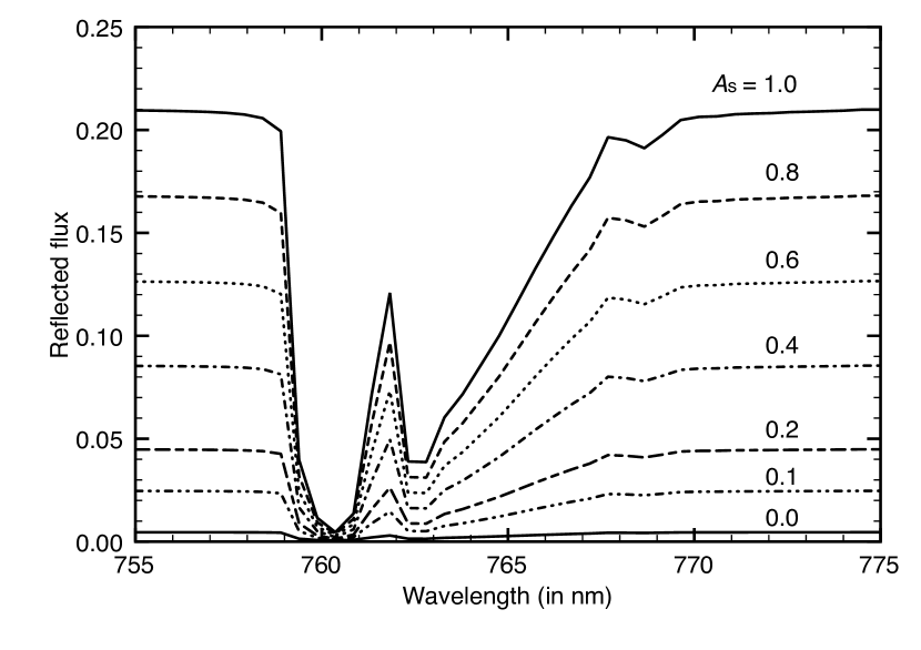
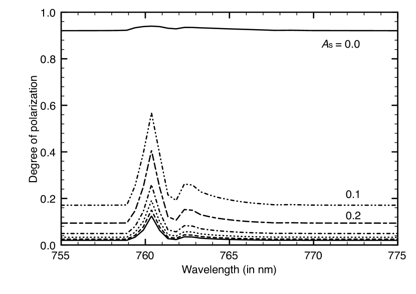
Figure 4: Flux $F$ (left) and degree of polarization $P_{\rm s}$ (right) of starlight reflected by cloud–free exoplanets at $\alpha=90^{\circ}$ for different surface albedo’s $A_{\rm s}$: 0.0 (thin solid line, cf. Fig. 3 and note the different polarization scale), 0.1 (dot–dot–dashed line), 0.2 (short - long dashed line), 0.4 (dot–dashed line), 0.6 (dotted line), 0.8 (dashed line), 1.0 (thick solid line).

3.1.1 The influence of the surface albedo $A_{\rm s}$

The first results to discuss are those for starlight reflected by model planets with gaseous, cloud–free atmospheres above surfaces with different albedo’s. Figure 4 shows $F$ and $P_{\rm s}$ for surface albedo’s $A_{\rm s}$ ranging from 0.0 to 1.0, at a phase angle $\alpha$ of $90^{\circ}$. This is a very advantageous phase angle for the direct detection of an exoplanet, because there its angular distance to its host star is largest. This phase angle also occurs at least twice every planetary orbit, independently of the orbital inclination angle.

For these cloud–free planets, $F$ and $P_{\rm s}$ in the continuum depend strongly on $A_{\rm s}$, because the atmospheric gaseous scattering optical thickness $b_{\rm sca}$ in this spectral region is very small (see Fig. 1). The continuum $P_{\rm s}$ decreases with increasing $A_{\rm s}$, because of the increasing contribution of unpolarized light that has been reflected by the surface to the planetary signal: even if $A_{\rm s}$ is only slightly larger than zero, the surface contribution already strongly influences this signal.

For these cloud–free planets with gaseous atmospheres, polarization $P_{\rm s}$ will increase with increasing $b_{\rm abs}$, because the contribution of multiple scattered light, with usually a low degree of polarization, to the planetary signal will decrease. Also, at wavelengths where the atmospheric absorption optical thickness $b_{\rm abs}$ is large (see Fig. 1), virtually no light will reach the surface to subsequently emerge from the top of the atmosphere. At those wavelengths, $F$ and $P_{\rm s}$ are insensitive to $A_{\rm s}$. In Fig. 4, $F$ and $P_{\rm s}$ in the deepest part of the absorption band (around 760.5 nm) do depend on $A_{\rm s}$, because they pertain to spectral bins and every bin includes wavelengths where $b_{\rm abs}$ is small, and thus light that has been reflected by the surface.

In exoplanet observations, absolute fluxes, such as shown in Fig. 4, might not be available because of missing knowledge about e.g. the planet radius, and/or the distances involved. Such observations could, however, provide relative fluxes, as shown in Fig. 5. For a cloud–free atmosphere, the relative depth of the absorption band appears to be very insensitive to $A_{\rm s}$, provided $A_{\rm s}>0.0$ (the curve for $A_{\rm s}=0.05$, which is not shown in the figure, would fall only slightly above that for $A_{\rm s}=0.1$). The curves in Fig. 5 pertain to horizontally homogeneous planets, but this insensitivity of the relative band depth to $A_{\rm s}$ also holds for cloud–free planets with a range of albedo’s across their surfaces.

This insensitivity of the relative band depth in flux can be explained by how the reflected flux varies with $b_{\rm abs}$, shown in Fig. 6. Because of the small values of $b_{\rm sca}$ in this spectral region, and thus the small amount of multiple scattering, the flux that reaches the surface and then the top of the atmosphere, depends almost linearly on $A_{\rm s}$ for every value of $b_{\rm abs}$. The insensitivity is thus independent of the spectral resolution. The slight increase of the relative band depth with increasing $A_{\rm s}$ visible in Fig. 5, is due to the slight increase in multiple scattered light and hence a slight increase of the absorption. With a higher surface pressure, and thus a larger $b_{\rm sca}$ and more multiple scattering, the relative band depth will show a larger sensitivity to $A_{\rm s}$.

Figure 6 also shows that in polarization spectra, the widths of individual absorption lines decrease with increasing surface albedo $A_{\rm s}$. The explanation for this narrowing of absorption lines in polarization spectra is that if for a given value of $b_{\rm abs}$, $A_{\rm s}$ is increased, more unpolarized light is added to the reflected starlight, decreasing $P_{\rm s}$ (see Eq. 13 in Stam et al., 1999).

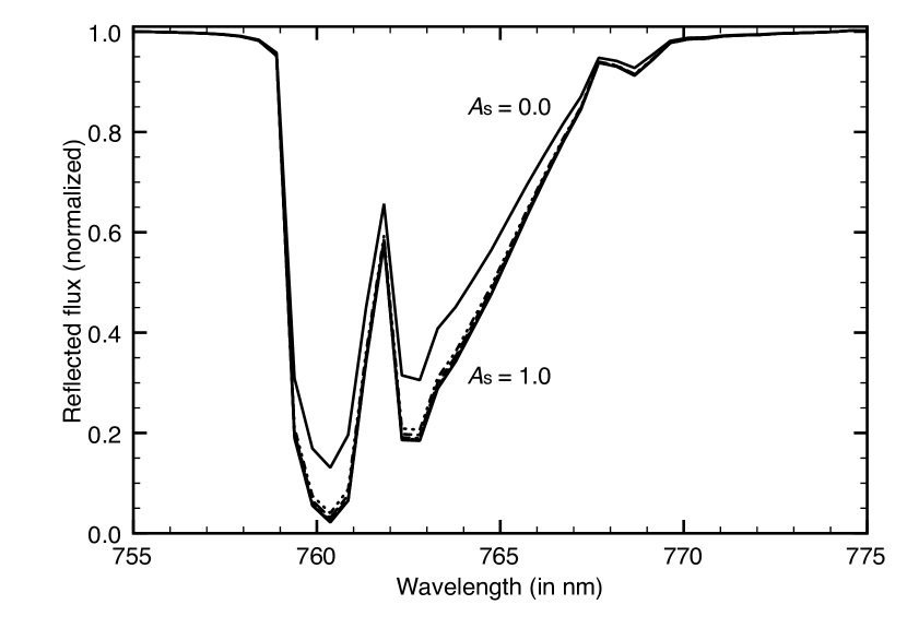
Figure 5: The reflected flux curves of Fig. 4 normalized at $\lambda=755$ nm. The shallowest band pertains to $A_{\rm s}=0.0$, and the deepest to $A_{\rm s}=1.0$.

3.1.2 The influence of the planetary phase angle $\alpha$

Figure 7 shows $F$ and $P_{\rm s}$ in the continuum (755 nm) as functions of the planetary phase angle $\alpha$, for different values of $A_{\rm s}$. For comparison, the curves for $b_{\rm abs}=400$ (the deepest absorption lines in the O₂ A–band) are also shown ($F$ is virtually zero). These curves (that are independent of $A_{\rm s}$) can be used to estimate the expected strength of individual absorption lines as compared to the continuum.

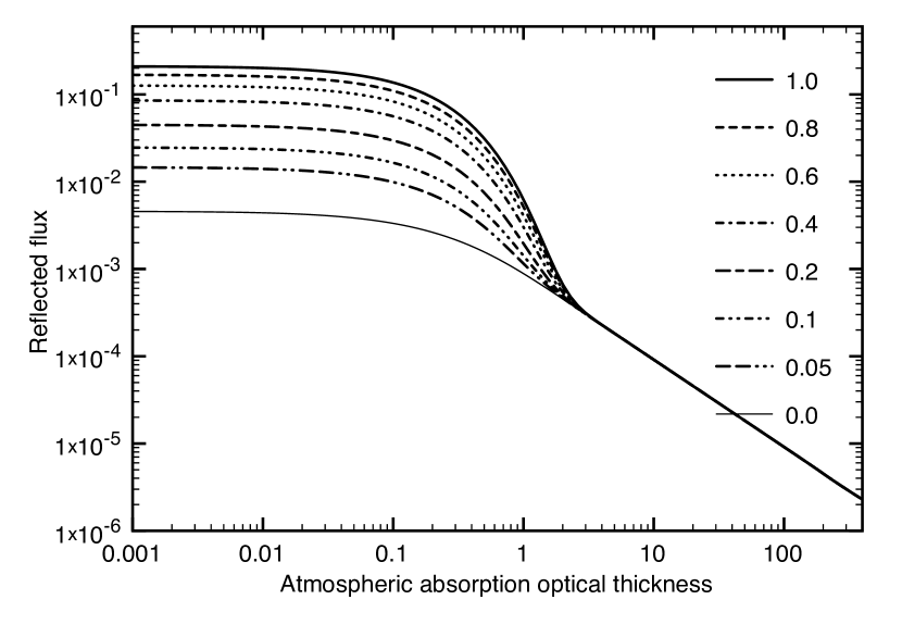
Figure 6: $F$ (left) and $P_{\rm s}$ (right) of starlight reflected by cloud–free exoplanets at $\alpha=90^{\circ}$ as functions of $b_{\rm abs}$ for different values of $A_{\rm s}$.

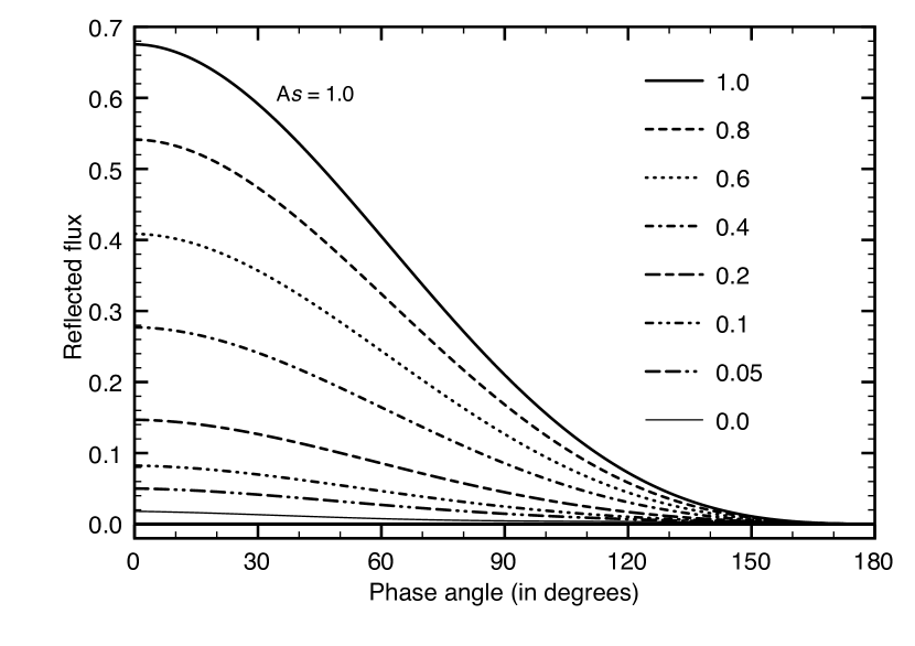
Figure 7: $F$ (left) and $P_{\rm s}$ (right) of starlight reflected at $\lambda=755$ nm (the continuum) by cloud–free exoplanets as functions of $\alpha$ for the same $A_{\rm s}$ as in Fig. 4, except with curves for $A_{\rm s}=0.05$ added. The thick solid curve peaking at $\alpha=93^{\circ}$ in $P_{\rm s}$ ($F$ is virtually zero) pertains to $b_{\rm abs}=400$.

The continuum $F$ decreases smoothly with increasing $\alpha$, while the continuum polarization curves have a maximum that shifts from 90^∘ when the surface is black, to larger values of $\alpha$ with increasing $A_{\rm s}$. Both for the planet with the black surface and for the planet with $b_{\rm abs}=400$, $P_{\rm s}$ peaks at or near $\alpha=90^{\circ}$, because for those planets the signal is mostly determined by light singly scattered by gas molecules (there is almost no multiple scattering in the atmosphere and there is no contribution from the surface), and at that phase angle, the scattering angle of the singly scattered light is 90^∘, precisely where Rayleigh scattered light has the highest polarization (see Fig. 2). At 755 nm, the model atmosphere has a very small gaseous scattering optical thickness, the reflected flux is thus mainly determined by $A_{\rm s}$, and the maximum of $P_{\rm s}$ decreases rapidly with increasing $A_{\rm s}$ and shifts to larger values of $\alpha$.

From the polarization curves in Fig. 7, it can be seen that for cloud–free planets with reflecting surfaces, the polarization inside the absorption band will be higher than in the continuum at all phase angles. For black planets and $60^{\circ}<\alpha<90^{\circ}$, $P_{\rm s}$ should be slightly lower inside the deepest absorption lines than in the continuum. However, as can be seen in Fig. 6 showing the flux and $P_{\rm s}$ as functions of $b_{\rm abs}$ at $\alpha=90^{\circ}$ for various values of $A_{\rm s}$, lower values of $P_{\rm s}$ will only occur in the deepest absorption lines (where the flux is extremely small). Thus, for cloud–free planets and without an absorption line–resolving spectral resolution, $P_{\rm s}$ in the band is expected to be higher than $P_{\rm s}$ in the continuum at all phase angles and for all $A_{\rm s}$.

3.1.3 The influence of the mixing ratio $\eta$

The strength of the O₂ A–band for a cloud–free atmosphere also depends on the O₂ mixing ratio $\eta$. Figure 6 gives insight in the influence of $\eta$, because $b_{\rm abs}$ depends linearly on $\eta$ (for a given surface pressure). To better illustrate the observable signals, Fig. 8 shows $F$ and $P_{\rm s}$ in the spectral bin covering the deepest part of the absorption band (around 760.4 nm), for $\eta$ up to 1.0 (a pure O₂ atmosphere) as functions of $A_{\rm s}$. The curve for $\eta=0.0$ equals the continuum. The phase angle is 90^∘.

Figure 8: $F$ (left), normalized to its continuum value, and $P_{\rm s}$ (right) of starlight reflected by cloud–free exoplanets in the deepest part of the O₂ A–band (the spectral bin around $\lambda=760.4$ nm), at $\alpha=90^{\circ}$, as functions of $A_{\rm s}$ for $\eta$ ranging from 0.0 (thick solid line, not shown in the flux as it equals 1.0) to 1.0 (long – short – short – long dashes) in steps of 0.1. The short dashed line represents $\eta=0.2$, closest to the Earth’s value.

The reflected flux curves in Fig. 8 show that 1. the band depth (i.e. 1.0 - curve) increases with increasing $\eta$, with saturation starting for $\eta>0.4$ independent of $A_{\rm s}$, and 2. the insensitivity of the band depth to $A_{\rm s}$ (see Fig. 5 for $\eta=0.21$) holds for all values of $\eta$, except for (near)–black surfaces. The polarization curves show that, with the 0.5 nm wide spectral bin, the band strength (i.e. $\mid$ curve - continuum $\mid$, with the continuum $P_{\rm s}$ given by the solid line in Fig. 8) is smallest when the surface is (near)–black for all $\eta$.

For a cloud–free planet with a depolarizing surface, high polarization is usually associated with low fluxes. The relation between the band strength in $P_{\rm s}$ and the band depth in the normalized $F$, derived from Fig. 8, is shown in the top–left of Fig. 9 (data for $\eta=0.0$ have been omitted). The plot clearly shows that the band depth in $F$ is most sensitive to $A_{\rm s}$ when the surface is dark ($A_{\rm s}<0.1$) and $\eta$ is small. Also, large polarization band strengths ($>0.5$) correlate with large band depths in $F$. Indeed, if one would measure a large band strength in $P_{\rm s}$ combined with a small band depth in $F$, one would have an indication that the planetary atmosphere contains clouds and/or haze particles in addition to the gaseous molecules (see Sect. 3.2).

The data points in Fig. 9 have been calculated assuming an Earth–like surface pressure and thus an Earth–like value for the atmospheric gaseous scattering optical thickness $b_{\rm sca}$. Calculations show that data points for other (still small) values of $b_{\rm sca}$ fall between those shown in Fig. 9: for a surface pressure (and hence $b_{\rm sca}$) twice as high as the Earth’s, the data points for, for example, $\eta=0.2$ are similar to those for $\eta=0.4$, except for slightly different values of $A_{\rm s}$. Thus, measuring a certain combination of band strength in $P_{\rm s}$ and band depth in $F$ without knowing the surface pressure and $A_{\rm s}$ would not directly allow the retrieval of $\eta$.

Figure 9: Scatter plot of $\Delta P$ versus $\Delta F$, with $\Delta P=P_{\rm 760.4~{}nm}-P_{\rm 755~{}nm}$ and $\Delta F=1.0-F_{\rm 760.4~{}nm}/F_{\rm 755~{}nm}$ ($F_{\rm x~{}nm}$ indicating the flux in the spectral bin around x nm). Data is shown for $\eta$ ranging from 0.1 to 1.0 in steps of 0.1 (not all values appear in all legends). Top–left: Data points derived from Fig. 8, thus for $A_{\rm s}$ equal to 0.0 (on the left of each line), 0.01, 0.02, 0.03, 0.04, 0.05, 0.1, 0.2, 0.4, 0.6, 0.8, and 1.0 (on the right of each line). Top-right; Data points derived from Fig. 12, thus for $b_{\rm cloud}$ equal to 0.0 (on the left of each line), 0.01, 0.1, 0.5, 1.0, 5.0, 10.0, 50.0, and 100.0. Bottom–left: Data points derived from Fig. 16, thus for cloud top altitudes equal to 2.0 (on the right of each line), 4.0, 6.0, 8.0, 10.0, 12.0 km (on the left of each line, note that we did not include flux band depths $<0.74$). Bottom–right: All data points from the other three plots combined.

3.2 Completely cloudy planets

3.2.1 The influence of the cloud optical thickness $b_{\rm cloud}$

The Earth has an average cloud coverage of about 60$\%$, with cloud optical thicknesses $b_{\rm cloud}$ ranging from almost 0 to over 100 in the visible (Marshak & Davis, 2005). Figure 10 shows the influence of $b_{\rm cloud}$ on $F$ and $P_{\rm s}$ in the continuum around the O₂ A–band as functions of $\alpha$, for $A_{\rm s}=0.0$. These curves show the background on which the absorption band could be measured. The cloud is a horizontally homogeneous layer of 2 km thick with its top at 6 km, embedded in the gaseous atmospheres of Sect. 3.1.

The curves in Fig. 10 show how increasing $b_{\rm cloud}$ brightens a planet at all phase angles, except for optically thin clouds ($b_{\rm cloud}\leq 1.0$), where the planets are darkest at $60^{\circ}<\alpha<90^{\circ}$. This is due to the single scattering phase function of the cloud particles (Fig. 2). This single scattering phase function is also the explanation for the ’primary rainbow’: the shoulder in $F$ and the local maximum in $P_{\rm s}$ around $\alpha=38^{\circ}$. The rainbow feature could help to identify water clouds on exoplanets (see e.g. Karalidi et al., 2012; Bailey, 2007).

The Rayleigh scattering polarization maximum around 90^∘, disappears with increasing $b_{\rm cloud}$, as the scattering by the cloud particles increasingly dominates the reflected signal. In particular, around $\alpha=90^{\circ}$, the single scattering polarization of cloud particles is almost zero (see Fig. 2). At small phase angles, $P_{\rm s}$ of the cloudy planets is negative, and the polarization direction is thus parallel to the reference plane. The directional change from parallel to perpendicular to the reference plane occurs around $\alpha=20^{\circ}$. Another directional change occurs at a larger phase angle: the larger $b_{\rm cloud}$, the closer this phase angle is to 80^∘ for the liquid water particles that form our clouds (see Fig. 2).

Figure 10: $F$ (left) and $P_{\rm s}$ (right) of starlight reflected at $\lambda=755$ nm (the continuum) by completely cloudy exoplanets with $A_{\rm s}=0.0$, as functions of $\alpha$. The optical thickness $b_{\rm cloud}$ (defined at 765 nm) varies from 0.01 to 50.0. The curves for cloud–free planets ($b_{\rm cloud}=0.0$) with a black and a white surface ($A_{\rm s}=1.0$) are also included. The cloud layer extends from 4 to 6 km.

Fig. 11 shows $F$ (normalized at 755 nm; for the absolute differences in the continuum flux, see Fig. 10) and $P_{\rm s}$ across the O₂ A–band for the same model planets, at $\alpha=90^{\circ}$. The flux band depth depends only weakly on $b_{\rm cloud}$, because of two opposing effects: 1. increasing $b_{\rm cloud}$ decreases the average photon path length (and thus the absorption), because more photons are scattered back to space, and 2. increasing $b_{\rm cloud}$ increases the average photon path length (and thus the absorption), through the increase of multiple scattering in the atmosphere. Which effect dominates, depends on the values of $b_{\rm abs}$ within a spectral bin, the illumination and viewing geometries, and the cloud micro- and macrophysical properties. For our model planets, the net effect is a flux band depth that is insensitive to $b_{\rm cloud}$.

This insensitivity holds for any O₂ mixing ratio $\eta$, as can be seen in Fig. 12, where we plotted $F$ and $P_{\rm s}$ in in the spectral bin covering the deepest part of the band as functions of $b_{\rm cloud}$ and $\eta$. Indeed, for $b_{\rm cloud}>1.0$ and $\eta>0.2$, the flux band depth is fairly constant with $b_{\rm cloud}$ for every $\eta$. Because of the insensitivity to $b_{\rm cloud}$, $\eta$ could be derived from the band depth of the normalized flux, although we would have to know the cloud top altitude (see Sect. 3.2.2).

The strength of the absorption band in $P_{\rm s}$ is sensitive for $b_{\rm cloud}$ up till about 5 (for larger $b_{\rm cloud}$ and $\eta=0.21$, the band has virtually disappeared). The continuum $P_{\rm s}$ decreases with increasing $b_{\rm cloud}$ (see also Fig. 10). $P_{\rm s}$ in the band also decreases, but at a different rate: at wavelengths where $b_{\rm abs}$ is large, the clouds are invisible and $P_{\rm s}$ will be high (see the $b_{\rm abs}=400$ line Fig. 7), while at wavelengths with little absorption, $P_{\rm s}$ will behave similarly as in the continuum. With unresolved absorption lines, as in Fig. 11, the band strength is a mixture of high and low polarization. According to Fig. 12, the $P_{\rm s}$ band strength (the absolute difference between each curve and the $\eta=0.0$ curve), increases with increasing $\eta$, yielding band strengths of tens of percents in $P_{\rm s}$.

Figure 9 includes a scatter plot based on Fig. 12, that shows the relation between the $P_{\rm s}$ band strength and the (normalized) $F$ band depth for various $b_{\rm cloud}$. Large $P_{\rm s}$ band strengths clearly correlate with large $F$ band depths. Thus, measuring a strong $P_{\rm s}$ band in combination with a shallow $F$ band at $\alpha=90^{\circ}$ would not be explainable by a cloud layer of liquid water particles. A reflecting surface instead of $A_{\rm s}=0.0$, would decrease $P_{\rm s}$ even more (except for very thick clouds, where $A_{\rm s}$ is irrelevant), and would thus not improve the explanation.

The previous discussion focused on $\alpha=90^{\circ}$. From Fig. 10, it can be seen that around $\alpha=38^{\circ}$, the continuum $P_{\rm s}$ of planets with optically thin clouds is higher than that of a cloud–free, black planet. Because with increasing $b_{\rm abs}$, the signals of all planets tend towards those of cloud–free planets, $P_{\rm s}$ inside the deepest lines of the O₂ A–band could be lower than in the weaker lines and the continuum for dark, e.g. ocean covered, planets with thin clouds, around $\alpha=38^{\circ}$. This can be seen in Fig. 13.

When absorption lines are not resolved, the effect will be smaller than shown in Fig. 13, because wavelengths with large $b_{\rm abs}$ will be mixed with wavelengths with small $b_{\rm abs}$. Figure 14 shows the band in $P_{\rm s}$ With our spectral bin width of 0.5 nm, at $\alpha=38^{\circ}$. For $b_{\rm cloud}=0.5$, $P_{\rm s}$ in the spectral bins with the strongest absorption lines is indeed lower than in adjacent bins, creating a band with a collapsed top. A non–zero surface albedo will lower the continuum $P_{\rm s}$ for planets with optically thin clouds, and diminish this inversion in the O₂ A–band. Figure 14 also shows the lack of a band feature on a cloud–free planet with a dark surface (because of the small $b_{\rm sca}$), and the difference in $P_{\rm s}$ of a planet with a thick cloud ($b_{\rm cloud}=50.0$) and a cloud–free planet with a white surface, that will have similar fluxes.

Figure 13 also shows that the widths of resolved absorption lines depend on $b_{\rm cloud}$. In $F$, optically thicker clouds narrow lines down for $0.1\leq b_{\rm abs}\leq 10$ as compared to those in the spectra of cloud–free planets. In $P_{\rm s}$, lines can exhibit various shapes: narrowed down (for $b_{\rm cloud}=50.0$), widened up with a tiny dip (0.01 or 1 %) when $b_{\rm abs}>4$ (for $b_{\rm cloud}=5.0$), or with higher $P_{\rm s}$ (0.02 or 2 %) at the edges, with a narrow dip starting at $b_{\rm abs}\approx 0.6$. The precise values of $b_{\rm abs}$ mentioned above depend on $\alpha$, as can be seen when comparing the curves for the cloud–free planet in Fig. 13 (with $\alpha=38^{\circ}$) with those in Fig. 6 (where $\alpha=90^{\circ}$). Examples of variations of line shapes in $P_{\rm s}$ in the presence of aerosol can be found in Stam et al. (1999).

Figure 11: $F$ (top) and $P_{\rm s}$ (bottom) of starlight reflected by exoplanets that are completely covered by clouds from 4 to 6 km of altitude with cloud optical thicknesses (defined at 765 nm) ranging from 0.0 (cloud–free) to 30. The flux curves have been normalized at 755 nm.

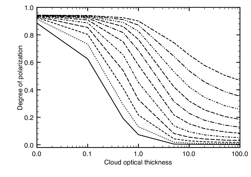
Figure 12: Similar to Fig. 8, except as functions of $b_{\rm cloud}$. The cloud is 2 km thick and has its top at 6.0 km. The surface is black and $\alpha=90^{\circ}$. The thick, solid line pertains to $\eta=0.0$.

3.2.2 The influence of the cloud top altitude $z_{\rm top}$

Because on Earth, the mixing ratio of O₂ is well–known and more or less constant with altitude, the depth of the O₂ A–band in the flux that is reflected to space can be used, to a first approximation, to derive the altitude of the top of a cloud layer. Indeed, this is the basis of several cloud top altitude retrieval techniques (Fischer & Grassl, 1991; Fischer et al., 1991). In this section, we investigate the relation between cloud top altitude, $z_{\rm top}$, and band depths and strengths for our model planets.

Figure 15 shows the (normalized) $F$ and $P_{\rm s}$ across the O₂ A–band for exoplanets with black surfaces that are completely covered by horizontally homogeneous clouds with $b_{\rm cloud}=10$ and $z_{\rm top}$ ranging from 2.0 to 10.0 km. The figure shows that the higher the cloud, the shallower the band in $F$. This is to be expected because the higher the cloud, the shorter the mean photon path through the atmosphere, and thus the less absorption. For the lowest cloud, the lowest (normalized) $F$ is only 6 % of the continuum. For the highest cloud, it is almost 20 % of the continuum. Interestingly, the $F$ band depth for the cloud–free planet is similar to that for a cloudy planet with $z_{\rm top}=6$ km. Because for the cloud–free planet with $A_{\rm s}=0.0$, only Rayleigh scattering contributes, its absolute flux will of course be much smaller than that of the cloudy planet (see Fig. 10). A cloud–free planet with $A_{\rm s}=1.0$, that would have a similar absolute flux as a cloudy planet, would have an $F$ band depth similar to that of the planet with $z_{\rm top}=2$ km (see Fig. 5).

The continuum $P_{\rm s}$ decreases with $z_{\rm top}$ and changes from perpendicular to parallel to the reference plane when $z_{\rm top}$ exceeds about 7 km (this altitude will depend on $b_{\rm cloud}$). The negative $P_{\rm s}$ is due to the negative single scattering polarization of the cloud particles at $\alpha=90^{\circ}$ (see Fig. 2), and the higher the clouds, the stronger their contribution to the planetary $P_{\rm s}$. Measurements by the POLDER–instrument (Deschamps et al., 1994) of the continuum polarization of sunlight reflected by regions on Earth are indeed being used to derive cloud top altitudes (Goloub et al., 1994; Knibbe et al., 2000), and a similar approach was used for cloud top altitude retrieval on Venus using Pioneer Venus orbiter data and sulfuric acid model clouds (Knibbe et al., 1998). Because of the abundance of photons in these Earth and Venus observations, high polarimetric accuracies can be reached. For example, the accuracy of POLDER is about 0.02 in degree of polarization (Toubbé et al., 1999).

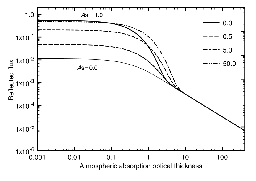
Figure 13: Similar to Fig. 6, except for $\alpha=38^{\circ}$, the ’rainbow’ angle, and $b_{\rm cloud}$ equal to 0.5, 5.0, and 50.0. For comparison, the curves for cloud-free planets with black and white surfaces have also been included.

The cloud top altitude also affects $P_{\rm s}$ in the band: the higher the cloud, the shallower the band. The reason for this change in band strength is that with increasing $z_{\rm top}$, the absorption optical thickness above the cloud decreases, and while $P_{\rm s}$ in the deepest absorption lines will remain high, it will decrease in the wings of these lines, see Fig. 14 for $\alpha=38^{\circ}$ (for optically thin clouds, it will increase when $\alpha=38^{\circ}$).

The effect of the O₂ mixing ratio $\eta$ on $F$ and $P_{\rm s}$ in the spectral bin covering the deepest part of the O₂ A–band, for various values of $z_{\rm top}$ is shown in Fig. 16 (recall that the continuum $F$ and $P_{\rm s}$ equal the case for $\eta=0.0$, only shown in the polarization plot). On Earth, the tops of optically thick clouds will usually not have $z_{\rm top}$ higher than about 14 km (except at equatorial latitudes where the tropopause can reach altitudes of about 18 km), but because cloud formation depends strongly on the atmospheric temperature profile, which will depend on the planet, we have included larger values for $z_{\rm top}$. It can be seen how the band depth in $F$ decreases with increasing $z_{\rm top}$: for $\eta>0.5$, $F$ in the band is close to zero unless $z_{\rm top}>10$ km, and thus insensitive to $z_{\rm top}$. There is an ambiguity between $z_{\rm top}$ and $\eta$: an observed band depth in $F$ could be fitted with different combinations of $z_{\rm top}$ and $\eta$. The band strength in $P_{\rm s}$ (i.e. the difference between the non–solid curves and the solid, $\eta=0.0$, curve), decreases with increasing $z_{\rm top}$, and is close to zero for small values of $\eta$ and/or $z_{\rm top}>12$ km. Here, there is a similar ambiguity, except that the smaller $\eta$, the smaller the maximum band strength in $P_{\rm s}$: large band strengths can only be explained by large $\eta$’s and/or low clouds.

The band strength in $P_{\rm s}$ as a function of the band depth in (normalized) $F$ is also shown in the lower left panel in Fig. 9. This figure makes clear that measuring both the band depth in $F$ and the band strength in $P_{\rm s}$ would allow the retrieval of both $z_{\rm top}$ and $\eta$, although that would require very accurate measurements and (in the absence of absolute flux and polarization measurements) assumptions about the planet’s surface albedo, especially with small values of $b_{\rm cloud}$, and the cloud coverage.

3.3 Partly cloudy planets

The model planets that we used previously, were either cloud–free or fully covered by a horizontally homogeneous cloud layer. These planets provide straightforward insight into the influence of clouds on the depth and strength of the O₂ A–band in, respectively, flux and polarization. The lower right panel of Fig. 9 contains all data points of the other panels, and thus shows the band strength in $P_{\rm s}$ as function of the band depth in $F$ for different values of $A_{\rm s}$, $\eta$, $b_{\rm cloud}$, and $z_{\rm top}$. The cloud of data points in this panel shows that the larger $\eta$, the larger the possible range of band depths in $F$ and band strengths in $P_{\rm s}$, and that for an Earth–like $\eta$ of 0.21, the band will show up in $P_{\rm s}$ only for dark (but not too dark) surfaces and optically thin clouds ($b_{\rm cloud}<5.0$) (at $\alpha=90^{\circ}$, and with our spectral bin width of 0.5 nm). A horizontally homogeneous planet is however an extreme case. Here, we will use horizontally inhomogeneous model planets, with patchy surfaces and patchy clouds, such as found on Earth.

For our horizontally inhomogeneous model planets, we use the following values for the surface albedo $A_{\rm s}$: 0.90 (representative for fresh snow), 0.60 (old and/or melted snow), 0.40 (sandy lands), 0.25 (grassy lands), 0.15 (forests), and 0.06 (oceans). Figure 17 shows an example of a (pixelated) cloud–free model planet, at $\alpha=90^{\circ}$, covered by five types of surfaces. The geometric albedo of this planet is 0.24.

All our surfaces are depolarizing, we thus do not include e.g. Fresnel reflection to describe the ocean surface. In Stam (2008), the disk–integrated signal of a cloud–free Earth–like planet with a flat Fresnel reflecting interface on top of a black surface (including glint) was found to have a $P_{\rm s}$ that was about 0.04 lower than that of the same planet without the Fresnel reflecting interface. For fully cloudy planets ($b_{\rm cloud}$=10), there was virtually no difference in the disk–integrated $P_{\rm s}$. Waves on the ocean surface would very likely reduce the influence of the Fresnel reflection, because of the randomizing effect of the variation in their directions, shapes and heights.

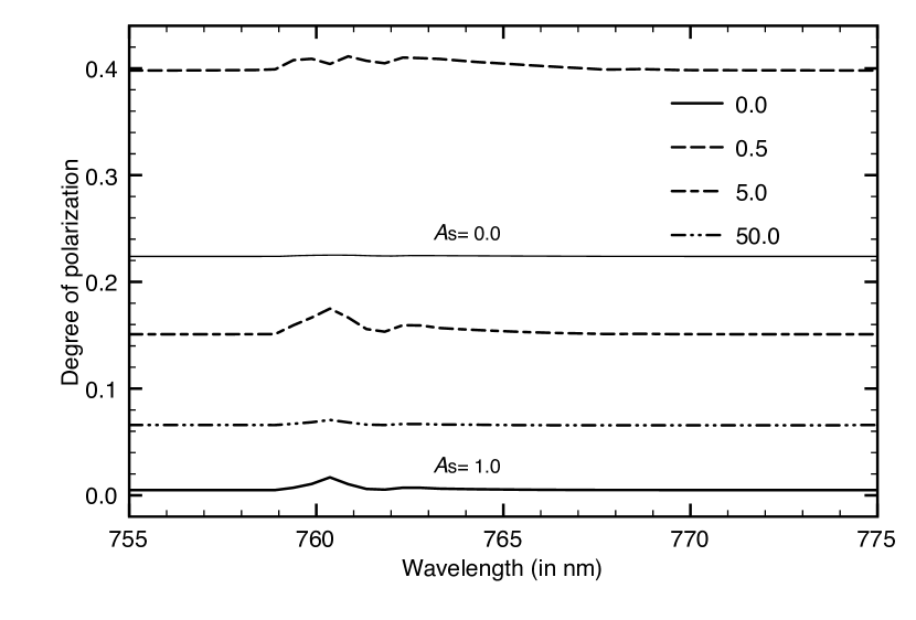
Figure 14: Similar to Fig. 12, except for $\alpha=38^{\circ}$, the ’rainbow’ angle, and $b_{\rm cloud}$ equal to 0.5, 5.0, and 50.0. For comparison, the curves for black ($A_{\rm s}=0.0$) and white ($A_{\rm s}=1.0$), cloud–free exoplanets have also been included.

Figure 15: $F$ (top) and $P_{\rm s}$ (bottom) of starlight reflected by planets that are completely covered by a horizontally homogeneous cloud layer with $b_{\rm cloud}=10$ that is 2 km thick. The cloud top altitude ($z_{\rm top}$ or CTA in the plot) ranges from 2.0 to 10.0 km. The red curves are for cloud–free planets with $A_{\rm s}=0.0$ (cf. Fig. 4). All flux curves have been normalized at 755 nm.

Figure 16: Similar to Fig. 8, except as functions of $z_{\rm top}$, for $b_{\rm cloud}=10$, a geometrical thickness of 2 km, and $A_{\rm s}=0.0$. The O₂ mixing ratio $\eta$ ranges from 0.0 (thick solid line, not shown in the flux as it equals 1.0) to 1.0, in steps of 0.1.

To model a patchy cloud pattern, we choose a cloud coverage (CC), i.e. the fraction of pixels that are cloudy. Note that these pixels are smaller than the pixels shown in Fig. 17. Next, we distribute an initial number of cloudy pixels (iCC, with iCC much smaller than the total number of cloudy pixels) randomly across the planetary disk. The remaining cloudy pixels are distributed across the remainder of the disk with the probability that a pixel will be cloudy increasing with the number of cloudy neighboring pixels. This method allows us to create patchy clouds with the size of the patches depending on the values of CC and iCC. In particular, the larger the difference between iCC and CC, the larger the patches. The user can assign different cloud properties ($b_{\rm cloud}$, $z_{\rm top}$, geometrical thickness, and particle micro–physics) to different cloudy pixels.

Figure 18 shows $F$ and $P$ of the heterogeneous model planet shown in Fig. 17 with cloud coverages equal to 0.0 (cloud–free), 0.5, and 1.0 (completely cloudy). The cloud properties are given in the figure caption. Not surprisingly, $F$ of the fully cloudy planet is higher than that of the cloud–free planet. The lowest $F$ is that of the partly cloudy planet, while one would expect a value in between the fluxes of the two other planets. Upon closer inspection, however, it appears that the poles of the partly cloudy planet are (partly) covered by clouds, suppressing $F$, because the clouds are less bright than the snow and ice surfaces. The polarization signal of the partly covered planet is between those of the other planets, because the polar regions do not contribute a significantly different polarization signal compared to the clouds.

Type	phase	$b_{\rm cloud}$	$z_{\rm bot}$ (km)	$z_{\rm top}$ (km)
1	liquid	0.2	4.0	6.0
2	liquid	5.0	4.0	6.0
3	liquid	10.0	4.0	6.0
4	liquid	50.0	4.0	6.0
5	liquid	10.0	6.0	8.0
6	solid	0.5	10.0	12.0

Table 1: The properties of the six model cloud types.

As already shown in Fig. 9, horizontally homogeneous planets present a wide variation in band strengths in $P$ versus band depths in $F$. Next, we will look at the variation that can be expected for horizontally inhomogeneous planets. In contrast to the curves in Fig. 18 which have been computed for a horizontally inhomogeneous planet with patchy clouds and surface albedo, for this, we will compute the variation of band strengths and depths by taking weighted sums of horizontally homogeneous planets to limit the computation times while maximizing the variations. Karalidi & Stam (2012) investigated the differences between ’true’ horizontal inhomogeneities and the weighted sum approach, and while for individual planets, the differences can be significant, statistically both methods yield the same results.

For a given value of $\eta$, we thus compute the flux vector of a planet using $\pi{\bf F}=(1/7)\Sigma_{i}^{7}\pi{\bf F}_{i}$, with ${\bf F}_{i}$ the flux vector of a horizontally homogeneous planet. The horizontally homogeneous planets used for the modeling can be either without clouds or completely covered by one of 6 cloud types. Table 1 shows the properties of the 6 cloud types. Types 1 - 5 consist of the same liquid water cloud particles that we used before. Type 6 consists of water ice crystals with scattering properties taken from Karalidi et al. (2012). We use the 6 surface albedo’s $A_{\rm s}$ specified in the caption of Fig. 17), and as before assume Lambertian surface reflection, because we are mainly interested in the effects of the clouds, and because the influence of a polarizing surfaces such as Fresnel reflection, is relatively small (Stam, 2008).

To avoid ending up with a huge number of data points, we decided to use a single value for $A_{\rm s}$ for each model planet, which still gives us 10348 flux vectors of planets. Figure 19 shows data points for $\eta=0.2$, 0.1, and 0.4. Several data points can be seen to line up, in particular the data points for cloud–free planets and planets with ice clouds. These lines of data points pertain to the ’transition’ from a homogeneous planet with a given surface albedo without clouds to a homogeneous planet with the same surface albedo but with clouds, with partially cloudy planets in between. Planets with optically thin clouds would fill the region between the densest part of the cluster of data points and the high $P$ points for the planets without clouds and with ice clouds (see also Fig. 9).

The data points in Fig. 19 clearly illustrate the variation of the band depth in $F$ for a single value of $\eta$ due to the differences in $A_{\rm s}$ and the cloud types. Although increasing $\eta$ generally increases the band depth in $F$, there is a huge overlap of data points for different values of $\eta$. When relatively small band depths in $F$ are observed, however, one would know that $\eta$ is small, even without knowledge on the presence of clouds and their properties or $A_{\rm s}$.

The vertical extend of the data points in Fig. 19 is a measure of the added value of measuring the band strength in $P$. The band strength could provide extra information about $b_{\rm cloud}$, the cloud coverage, and $A_{\rm s}$, in particular for optically thinner clouds. As can be seen, for higher values of $\eta$, the range of band strengths and thus the added value of $P$ increases strongly at this phase angle of 90^∘. Conversely, large band strengths in $P$ combined with large band depths in $F$ would indicate high values of $\eta$.

The model planets that provided the data points for Fig. 19 are quasi–horizontally inhomogeneous: their $F$ and $P$ values are representative for horizontally inhomogeneous planets, but they do not account for, for example, the effects of localized and patchy clouds (the spectra in Fig. 18 do account for these effects). In Fig. 20, we illustrate the variation in the band depth in $F$ and the band strength in $P$ for planets with homogeneous surfaces ($A_{\rm s}=0.15$ or 0.6) and patchy clouds of the types 1, 5, and 6 (the ice clouds). Each planet has one type of clouds. Given a planet with a certain cloud coverage, we computed $F$ and $P$ for 200 randomly selected different shapes and locations of the cloud patches (this method is described in detail in Rossi & Stam (2017)). The error bars indicate the 1–$\sigma$ variability in the computed signals for each planet (the variability equals zero for the fully cloudy planets).

Figure 17: Our model planet with its heterogeneous surface, and without clouds, at $\alpha=90^{\circ}$. The colors of the pixels represent the following surface types: White = fresh snow regions (32 pixels @ $A_{\rm s}$=0.9); light–grey = old and/or melted snow (15 pixels @ $A_{\rm s}$= 0.6); light–green = grassy lands (39 pixels @ $A_{\rm s}$= 0.25); dark–green = forests (50 pixels @ $A_{\rm s}$= 0.15); yellow = sandy desert (30 pixels @ $A_{\rm s}$= 0.4); blue = ocean (150 pixels @ $A_{\rm s}$= 0.06).

Figure 18: Similar to Fig. 15, except for the heterogeneous model planet shown in Fig. 17 ($\alpha=90^{\circ}$) without clouds (CC= 0.0), with half of the pixels covered by clouds (CC=0.5) and with all pixels covered by clouds (CC=1.0). The clouds have the following properties: 50% with $b_{\rm cloud}=50$, 16.7% with $b_{\rm cloud}=5$, 16.7% with $b_{\rm cloud}=10$, all between 4 and 6 km altitude, 16.5% with $b_{\rm cloud}=10$, between 8 and 10 km.

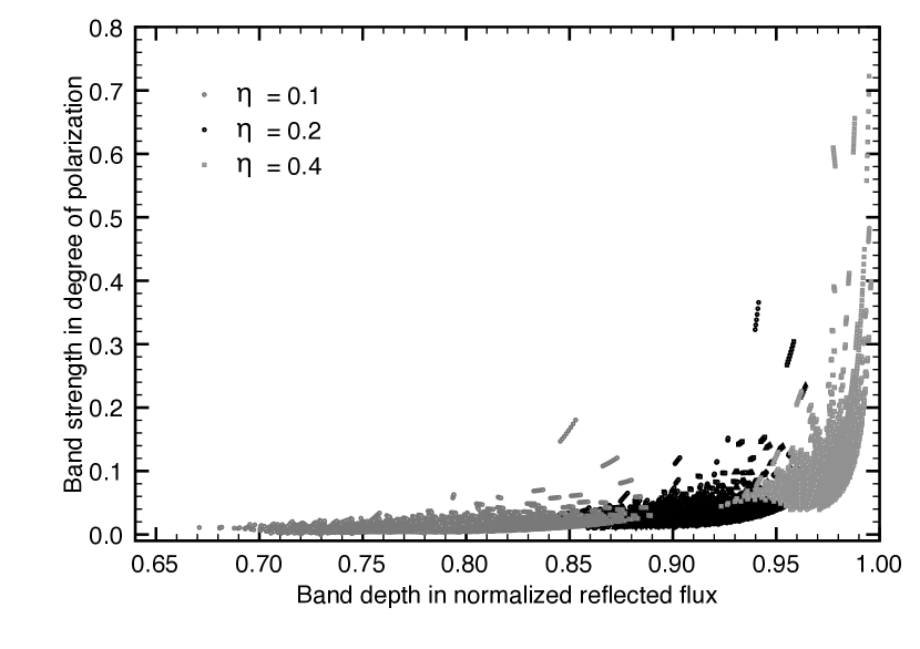
Figure 19: Similar to Fig. 9 for $\eta=0.2$ (left) and $\eta=0.1$, $0.2$, and 0.4 (right), $\alpha=90^{\circ}$. Each model planet has 6 possible values of $A_{\rm s}$, cloud–free and/or cloudy pixels (of the 6 types in Tab. 1). Left: the white symbols pertain to horizontally homogeneous planets. The small, dark symbols pertain to horizontally inhomogeneous planets. Right: the data points for $\eta=0.2$ partially over–plotted by those for $\eta=0.1$ (on the left side) and 0.4 (on the right side).

Figure 20 shows that for a given cloud coverage CC and type, the actual distribution of the clouds across the planetary disk usually also influence the bands in $F$ and $P$. The variability decreases with increasing CC, because a large amount of clouds allows less spatial variation. Above a dark surface ($A_{\rm s}=0.15$), high altitude, liquid water clouds with $b_{\rm cloud}=10$ (type 5, bottom left), show a smaller variance in both $P$ and $F$ than thin, low altitude clouds (type 1, top left). Increasing the surface albedo of the latter planet (top right) decreases the variability both in $P$ and in $F$ for all cloud coverages, while not strongly changing the average values. The spatial distribution of the thin, high altitude ice clouds (type 6, bottom right) has a negligible influence on the bands, for every $\eta$.

The large number of free parameters on a planet introduces significant degeneracies in the relation between band depths in $F$ and band strengths in $P$. A detailed investigation of the data points and the underlying planet models as shown in Figs. 19 and 20 not only at $\alpha=90^{\circ}$ but also at other phase angles, and across a wider wavelength region (in particular, including shorter wavelengths that are more sensitive to the gas above the clouds) could lead to the development of a retrieval algorithm for future observations, but is outside of the scope of this paper.

4 Discussion

The detection of absorption bands and the subsequent determination of column densities or mixing ratios of atmospheric biosignatures such as O₂, H₂O and CH₄ are crucial tools in the search for habitable environments and life on exoplanets. The strength of a gaseous absorption band in a visible planetary spectrum depends on the mixing ratio of the gas under investigation, on other atmospheric constituents and vertical structure, and on the surface properties.

On Earth, oxygen arises from large–scale photosynthesis and is well–mixed up to high altitudes. Because we have detailed knowledge about the Earth’s O₂ mixing ratio and vertical distribution, a routine Earth–observation method for determining cloud top altitudes is the measurement of the depth of the O₂ A–band in the flux of sunlight that is reflected by completely cloudy regions (see Saiedy et al., 1965; Vanbauce et al., 1998; Koelemeijer et al., 2001; Preusker et al., 2007; Lelli et al., 2012; Desmons et al., 2013, etc.). Knowledge of cloud top altitudes is important for climate studies and also to determine the mixing ratios of gases like ozone, H₂O and CH₄, that are strongly altitude dependent, and whose spectral signatures are also affected by the presence and properties of clouds. For exoplanets, cloud parameters and mixing ratios are unknown, and the aim is to determine both.

Our computations show that there will be significant degeneracies if only fluxes of reflected starlight are being used. Assuming that a planet is horizontally homogeneous, and observed at a phase angle of 90^∘, a measured absorption band depth in flux $F$ could be fitted with different O₂ mixing ratios $\eta$ depending on the assumed cloud optical thickness (Fig. 12) and cloud top altitude (Fig. 16). The surface albedo appears to be less of an influence (Fig. 5). Here, we assumed that only the relative fluxes are available, because absolute exoplanet fluxes can only be obtained when the planet radius and distances to its star and observer are known (the flux of a small bright planet can equal that of a large dark planet).

Degeneracies are even more of a problem if the planet is assumed to be horizontally inhomogeneous. Our computations for planets with different mixing ratios, and patchy clouds with various coverage percentages and spatial distributions, optical thicknesses and altitudes, and thermodynamical phase (liquid or ice; the phase could be derived from the cloud altitude if the atmospheric temperature profile is known), show a wide range of band depths in the flux with significant overlap between the signals of various model planets. Including surface pressures different than that on Earth, clouds made of other condensates than water, and atmospheric hazes and/or other aerosol, would increase the range of possible fits to the observations.

Measuring both the flux and the polarization of starlight that is reflected by a planet could help to reduce the degeneracies, because the band strength in polarization has a different sensitivity to the atmospheric parameters and the surface albedo than the band depth in reflected flux. Indeed, assuming a horizontally homogeneous planet, and a phase angle of 90^∘, measuring $P$ would help to retrieve the cloud optical thickness, although for optically thin clouds, the surface albedo would influence the signal, too. The sensitivity of the polarization does depend on the mixing ratio: the larger $\eta$, the larger the range of $b_{\rm cloud}$ polarimetry is sensitive to. The polarization also holds information on the cloud top altitude, although the mixing ratio should be known for an actual retrieval. Here, a combination with flux measurements could help. Retrieving cloud top altitudes with an error of $\pm 2$ km would require polarization measurements with a precision of 1 – 2$\%$.

Assuming horizontally inhomogeneous planets, the range of planet parameters that would fit a certain combination of flux and polarization measurements obviously increases. To diminish degeneracies, the observational precision should be increased, as subtle differences in flux and polarization could help to distinguish between different models. Measurements at several phase angles would also provide more information, as in particular the degree of polarization in and outside the band depend strongly on the atmospheric parameters. Indeed, measurements at the rainbow phase angle (38^∘) would not only help to determine whether cloud particles are made of liquid water, but also provide information on the cloud optical thickness. Hansen & Travis (1974) show a number of plots of the single scattering polarization of particles with different compositions. An investigation into what would be the distinguishing ’rainbow’ phase angle for clouds made of such particles would help to plan observations, but is outside the scope of this paper.

Another method to diminish degeneracies would be to perform observations at a range of wavelengths, in particular, short wavelengths are more sensitive to scattering by gas and small particles than longer wavelengths, and could thus provide more information about the amount of gas above the clouds (i.e. the cloud top altitude), and possibly about the cloud patchiness (by reflecting more light from the cloud–free regions). Longer wavelengths are less scattered by the gas and small particles, and thus give a better view of the clouds and surfaces. Because of the spectral information in both the flux and the polarization, not only in absorption bands but also in the continuum, it is thus essential to use narrow band observations rather than broadband observations.

A high temporal resolution would also help to identify the contributions of time varying signals such as the rotation of a planet with a horizontally inhomogeneous surface (a regular variation, not addressed in this paper) and/or weather patterns changing the cloud coverage (as on Earth, the cloud coverage could also depend on the surface properties, such as the presence of mountains). Our computations of the variability in the O₂ A–band depth and strength in flux and polarization due to different shapes and locations of cloud patches (Fig. 20) illustrate which observational accuracy would be needed to resolve such variations, which depend on the cloud coverage and the mixing ratio.

In our models, the surfaces reflect Lambertian, i.e. depolarizing. Various types of natural surfaces reflect linearly polarized light, and sometimes also circularly polarized (see, e.g. Patty et al., 2017, and references therein). Including such polarizing surfaces into our planet models would strongly increase the number of free parameters, and while the influence of the polarizing surfaces could influence the continuum polarization for the regions on a planet that are cloud–free with at most a few percent provided the surface albedo is not too low (see Stam, 2008, for results for a planet completely covered by a flat, Fresnel reflecting ocean surface). For cloudy regions no influence of the surface polarization is expected.

While our computations show that measuring the polarization would decrease the degeneracies in retrievals of mixing ratios of gases such as the biosignature O₂, they can also be used to optimize the design of instruments and/or telescopes. Indeed, many spectrometers are sensitive to the polarization of the observed light: the measured flux will depend on the polarization of the incoming light. Because the polarization will usually vary across a gaseous absorption band, any instrumental polarization sensitivity will change the shape and depth of measured absorption bands. Unless carefully corrected for (which is difficult when the incoming polarization is not known, even when the instrumental polarization is accurately known), such changes will influence the retrieved gas mixing ratios. Typical absorption band strengths in our polarization computations can be combined with (estimated) instrumental polarization sensitivities to estimate and possibly minimize the errors that could result.

These errors will strongly depend on the spectral resolution of the observations: the higher the spectral resolution, the higher the observable degree of polarization. This can be seen in Fig. 3 and also in the various figures that show $F$ and $P$ (or $P_{\rm s})$ as functions of $b_{\rm abs}$, the atmospheric absorption optical thickness. Thus the higher the spectral resolution, the more information can be obtained from observations, but the more care should be taken to account for instrumental polarization.

Current large ground–based telescopes with broadband photometric and polarimetric capabilities for exoplanet observations are SPHERE/VLT and GPI/Gemini North. Narrow–band spectropolarimetry might become available in the near–future on EPICS/ELT and proposed space–telescopes such as WFIRST, LUVOIR or HabEX, and provide us with the first spectra of the O₂ A–band to be used for the characterization of exoplanets (absorption line resolving Doppler detections of exoplanetary O₂ might indeed succeed earlier and provide lower limits for the O₂ column density). Then the difficulty will be to discard false–positives detections of O₂. Indeed, for instance, dioxygen may not necessarily be a biosignature (Wordsworth & Pierrehumbert, 2014; Domagal et al., 2014; Harman et al., 2015; Schwieterman et al., 2016, 2016b). Lifeless, terrestrial planets in the habitable zone of any type of star can develop oxygen–dominated atmospheres through photolysis of H₂O (e.g. Wordsworth & Pierrehumbert, 2014) or CO₂ (e.g. Harman et al., 2015). However, O₂ due to CO₂ photolysis would not be detectable with current and planned space– and ground–based instruments on planets around F and G type stars. Planets around K–stars and especially M-stars, may produce detectable abiotic O₂ because of the low UV–flux from their parent stars (Harman et al., 2015). Also, strong O₄ features that could be visible in transmitted spectra at 1.06 and 1.27 $\mu$m or in UV/VIS/NIR reflected light spectra by a next generation direct–imaging telescopes such as LUVOIR/HDST or HabEx could be a sign of an abiotic dioxygen–dominated atmosphere that suffered massive H–escape (see Schwieterman et al., 2016, 2016b). These considerations highlight the importance of wide spectral coverage for future exoplanet characterization missions (Domagal et al., 2014), and the combination of flux and polarization measurements in order to obtain as much information as possible from the limited numbers of photons.

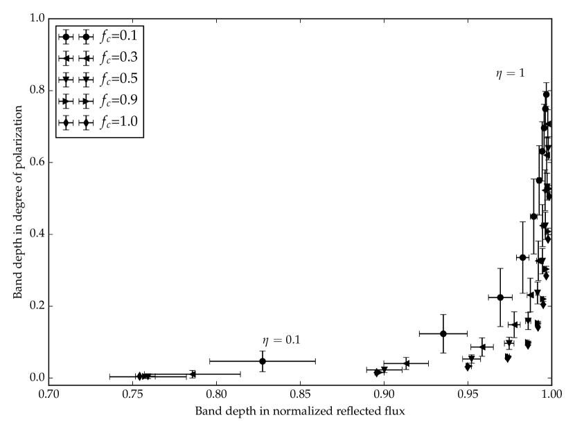
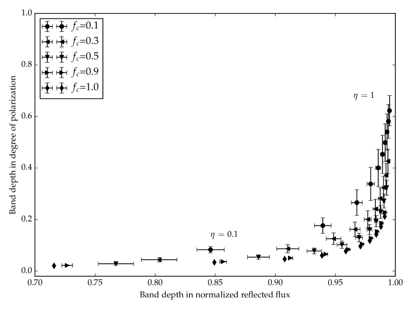
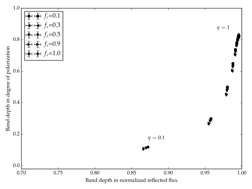
Figure 20: Similar to Fig. 19 except for planets with patchy clouds, and $\alpha=90^{\circ}$. Each planet has one value for $A_{\rm s}$ and one cloud type (see Tab. 1). Top left: $A_{\rm s}=0.15$, type 1. Top right: $A_{\rm s}=0.6$, type 1. Bottom left: $A_{\rm s}=0.15$, type 5. Bottom right: $A_{\rm s}=0.15$, type 6 (ice clouds). The error bars indicate the variance in the band depth in $F$ and in the band strength in $P$ for the same value of CC ($f_{\rm c}$ in the plot), but for different distributions of the clouds. Mixing ratio $\eta$ increases from 0.1 to 1.0 in steps of 0.1.

5 Summary

We have computed the O₂ A–absorption band feature in flux and polarization spectra of starlight that is reflected by Earth–like exoplanets and investigated its dependence planetary parameters. The O₂ A–band covers the wavelength region from about 755 to 775 nm, and it is the strongest absorption band of diatomic oxygen in the visible. Observations of the depth of this band in the reflected flux and the strength of the band in polarization could be used to derive the O₂ mixing ratio in the atmosphere of an exoplanet and with that provide insight into the possible level of photosynthetic processes on the planet.

In our model computations, we assumed that O₂ is well–mixed and that the clouds on a planet consist of water, like on Earth. We varied the O₂ mixing ratio $\eta$, the planetary surface albedo $A_{\rm s}$, the cloud optical thickness $b_{\rm cloud}$, the cloud top altitude $z_{\rm top}$, and the cloud fraction and spatial distribution over the planet. We computed both the flux $F$ and the degree of linear polarization $P$ (or $P_{\rm s}$) of the starlight that is reflected by the model planet. Because of the difficulty of measuring absolute fluxes and polarization of exoplanets (and without accurate knowledge of the distance to an exoplanet and its size, a measured reflected flux cannot be directly related to the albedo of the planet), we focus on the relative difference between $F$ in the deepest part of the O₂ A–band (around 760.4 nm) and in the continuum outside the band (at 755 nm), with the latter normalized to one. For $P$, which is independent of distances and planetary radii because it is a relative measure, we focus on the absolute difference between the polarization in the deepest part of the band and that in the continuum. We use a spectral bin width of 0.5 nm for the spectral computations, but values for narrower bins can be derived from computations of $F$ and $P$ as functions of the atmospheric absorption optical thickness.

While, as expected, $F$ in the band is always smaller than $F$ in the surrounding continuum, $P$ in the band is higher than in the continuum in most of our model computations, with strong variations in the band strength depending on the atmospheric and surface parameters. For absorption line resolving observations, $P$ will show even more variation with respect to its continuum value, especially in the deepest absorption lines and with vertical structure in the atmosphere, such as the presence of high altitude ice clouds.

Our computations lead us to the following main conclusions:

$\bullet$ For $\alpha=90^{\circ}$ and a given value of $\eta$, the band depth in (relative) $F$ is very insensitive to the surface albedo $A_{\rm s}$ if it is larger than about 0.1, and the cloud optical thickness $b_{\rm cloud}$ if it is larger than about 0.5.

$\bullet$ For $\alpha=90^{\circ}$, the band depth in (relative) $F$ is sensitive to the cloud top altitude $z_{\rm top}$, although the sensitivity decreases for $\eta>0.2$ and $z_{\rm top}<10$ km).

$\bullet$ The band strength in $P$ is very sensitive to $A_{\rm s}$, except when $\eta>0.7$, and for $30^{\circ}<\alpha<150^{\circ}$. If $A_{\rm s}\approx 0$, the band strength is smaller than 0.04 (for a spectral bin width of 0.5 nm).

$\bullet$ The band strength in $P$ is very sensitive to $b_{\rm cloud}$ as long as $b_{\rm cloud}$ is smaller than about 5 for $\eta=0.2$. The band strength increases with $\eta$. If $\eta=0.2$ and $b_{\rm cloud}>5$, the band strength is smaller than 0.04 (for 0.5 nm wide bins, and $\alpha=90^{\circ}$).

$\bullet$ The band strength in $P$ decreases with $z_{\rm top}$. For $\eta=0.2$, the maximum band strength (for $z_{\rm top}=2$ km) is about 0.10 at $\alpha=90^{\circ}$.

$\bullet$ For partly cloudy planets with or without horizontally inhomogeneous surface albedo’s below the atmosphere, the degeneracies are even larger. Variations in $F$ and $P$ measured over time, could help to identify whether observed band depths and strengths are due to clouds or surface features.

$\bullet$ Measuring both $F$ and $P$ appears essential to reduce the existing degeneracies due to the effects of the surface albedo, cloud optical thickness and altitude, and O₂ mixing ratios. Increasing the wavelength coverage (short and long wavelengths) and the phase angle range of the observations will also help to reduce degeneracies. In particular, phase angles close to the rainbow angle, i.e. $38^{\circ}$, would not only help with identifying the presence of liquid water particles but the strength of the O₂ A–band in polarization at that phase angle can be used for cloud optical thickness retrieval.

$\bullet$ The band depth in $F$ will increase and the band strength in $P$ will become stronger (in vertically homogeneous atmospheres), with increasing spectral resolution, i.e. increasing spectral bin width. Absorption–line resolving observations of $P$ would reveal a large variation of the behavior of $P$ across the deepest absorption lines, in particular in the presence of high–altitude clouds or hazes.

The O₂ A–band is the strongest spectroscopic feature of dioxygen detection in reflected starlight. The retrieval of $O_{2}$ mixing ratio will be difficult due to degeneracies that can occur for various combinations of cloud optical thickness, cloud altitude, (similarly for hazes) and surface properties. Cloud composition, which we haven’t included in our study, would also play a role. To reduce the degeneracies, the flux and the polarization should be used together to provide information on the cloud optical thickness, in particular if measured at a range of phase angles and wavelengths.

6 Acknowledgments

We would like to thank the anonymous reviewer for the elaborate comments that allowed us to improve the quality of this paper. This work was initiated a the LOA, Lille 1 University and completed during Thomas Fauchez NASA Postdoctoral Program (NPP). This paper is not funded or sponsored by NASA.

References

- Aben et al. (2001) Aben, I., Stam, D. M., & Helderman, F. 2001, Geophys. Res. Lett., 28, 519
- Anglada-Escudé et al. (2016) Anglada-Escudé, G., Amado, P. J., Barnes, J., et al. 2016, Nature, 536, 437
- Bailey (2007) Bailey, J. 2007, Astrobiology, 7, 320
- Beuzit et al. (2006) Beuzit, J.-L., Feldt, M., Dohlen, K., et al. 2006, The Messenger, 125, 29
- Boesche et al. (2008) Boesche, E., Stammes, P., Preusker, R., et al. 2008, Appl. Opt., 47, 3467
- Bott et al. (2016) Bott, K., Bailey, J., Kedziora-Chudczer, L., Cotton, D. V., Lucas, P. W., Marshall, J. P., & Hough, J. H., 2016, MNRAS, 459, L109
- Crowe et al. (2013) Crowe, S., Døssing, L., Beukes, N., et al. 2013, Nature, 501, 535
- de Haan et al. (1987) de Haan, J. F., Bosma, P. B., & Hovenier, J. W. 1987, A&A, 183, 371
- de Rooij & van der Stap (1984) de Rooij, W. A. & van der Stap, C. C. A. H. 1984, A&A, 131, 237
- Deschamps et al. (1994) Deschamps, P. Y., Bréon, F. M., Leroy, M., et al. 1994, IEEE Trans. Geosci. Remote Sens., 32, 598
- Desmons et al. (2013) Desmons, M., Ferlay, N., Parol, F., Mcharek, L., & Vanbauce, C. 2013, Atmospheric Measurement Techniques Discussions, 6, 2533
- Domagal et al. (2014) Domagal-Goldman, S. D., Segura, A., Claire, M. W., Robinson, T. D., & Meadows, V. S. 2014, ApJ, 792, 90
- Ferlay et al. (2010) Ferlay, F., Thieuleux, F., & Cornet, C. 2010, J. Appl. Meteor. Climatol., 49, 2492
- Fischer et al. (1991) Fischer, J., Cordes, W., Schmitz-Peiffer, A., Renger, W., & Mörl, P. 1991, Journal of Applied Meteorology, 30, 1260
- Fischer & Grassl (1991) Fischer, J. & Grassl, H. 1991, Journal of Applied Meteorology, 30, 1245
- Fougnie et al. (2007) Fougnie, B., Bracco, G., Lafrance, B., et al. 2007, Appl. Opt., 46, 5435
- Froning et al. (2006) Froning, C., Osterman, S., Beasley, M., Green, J., & Beland, S. 2006, Proc. SPIE, 6269, 62691V
- Fujii et al. (2013) Fujii, Y., Turner, E. L., & Suto, Y. 2013, ApJ, 765, 76
- Gisler et al. (2004) Gisler, D., Schmid, H. M., Thalmann, C., et al. 2004, in Presented at the Society of Photo-Optical Instrumentation Engineers (SPIE) Conference, Vol. 5492, Ground-based Instrumentation for Astronomy. Edited by Alan F. M. Moorwood and Iye Masanori. Proceedings of the SPIE, Volume 5492, pp. 463-474 (2004)., ed. A. F. M. Moorwood & M. Iye, 463–474
- Goloub et al. (1994) Goloub, P., Deuze, J. L., Herman, M., & Fouquart, Y. 1994, IEEE Transactions on Geoscience and Remote Sensing, 32, 78
- Goloub et al. (2000) Goloub, P., Herman, M., Chepfer, H., et al. 2000, J. Geophys. Res., 105, 14
- Gratton et al. (2011) Gratton, R., Kasper, M., Vérinaud, C., Bonavita, M., & Schmid, H. M. 2011, in IAU Symposium, Vol. 276, IAU Symposium, ed. A. Sozzetti, M. G. Lattanzi, & A. P. Boss, 343–348
- Groff et al. (2014) Groff, T. D., Peters, M., Kasdin, N. J., et al. 2014, in American Astronomical Society Meeting Abstracts, Vol. 223, American Astronomical Society Meeting Abstracts 223, 148.34
- Hansen & Hovenier (1974) Hansen, J. E. & Hovenier, J. W. 1974, J. Atmos. Sci., 31,1137
- Hansen & Travis (1974) Hansen, J. E. & Travis, L. D. 1974, Space Science Reviews, 16, 527
- Harman et al. (2015) Harman, C. E., Schwieterman, E. W., Schottelkotte, J. C., & Kasting, J. F. 2015, ApJ, 812, 137
- Hovenier et al. (2004) Hovenier, J. W., van der Mee, C. V. M., & Domke, H. 2004, Transfer of Polarized Light in Planetary Atmospheres; Basic Concepts and Practical Methods (Kluwer, Dordrecht; Springer, Berlin)
- Hovenier & van der Mee (1983) Hovenier, J. W., van der Mee, C. V. M., 1983, A&A, 128, 1
- Joos & Schmid (2007) Joos, F. & Schmid, H. M. 2007, A&A, 463, 1201
- Kaltenegger & Traub (2009) Kaltenegger, L. & Traub, W. A. 2009, ApJ, 698, 519
- Karalidi & Stam (2012) Karalidi, T., & Stam, D. M., 2012, A&A, 546, A56
- Karalidi et al. (2012) Karalidi, T., Stam, D. M., & Hovenier, J. W. 2012, A&A, 548, A90
- Kasting et al. (1993) Kasting, J. F., Whitmire, D. P., & Reynolds, R. T. 1993, Icarus, 101, 108
- Kawata (1978) Kawata, Y. 1978, Icarus, 33, 217
- Keller (2006) Keller, C. U. 2006, in Presented at the Society of Photo-Optical Instrumentation Engineers (SPIE) Conference, Vol. 6269, Ground-based and Airborne Instrumentation for Astronomy. Edited by McLean, Ian S.; Iye, Masanori. Proceedings of the SPIE, Volume 6269, pp. 62690T (2006).
- Keller et al. (2010) Keller, C. U., Schmid, H. M., Venema, L. B., et al. 2010, in Society of Photo-Optical Instrumentation Engineers (SPIE) Conference Series, Vol. 7735, Society of Photo-Optical Instrumentation Engineers (SPIE) Conference Series
- Kemp et al. (1987) Kemp, J. C., Henson, G. D., Steiner, C. T., & Powell, E. R. 1987, Nature, 326, 270
- Kemp (1971) Kemp,J. C., Wolstencroft, R. D., 1971, Nature, 232, 165
- Knibbe et al. (2000) Knibbe, W. J. J., de Haan, J. F., Hovenier, J. W., et al. 2000, J. Quant. Spec. Radiat. Transf., 64, 173
- Knibbe et al. (1998) Knibbe, W. J. J., de Haan, J. F., Hovenier, J. W., & Travis, L. D. 1998, J. Geophys. Res., 103, 8557
- Koelemeijer et al. (2001) Koelemeijer, R. B. A., Stammes, P., Hovenier, J. W., & de Haan, J. F. 2001, Journal of Geophysical Research: Atmospheres, 106, 3475
- Konopacky et al. (2013) Konopacky, Q. M., Barman, T. S., Macintosh, B. A., & Marois, C. 2013, Science, 339, 1398
- Lacis & Oinas (1991) Lacis, A. A., & Oinas, V., 1991, J. Geophys. Res., 96, 9027
- Lelli et al. (2012) Lelli, L., Kokhanovsky, A. A., Rozanov, V. V., et al. 2012, Atmospheric Measurement Techniques, 5, 1551
- Lindstrot et al. (2006) Lindstrot, R., Preusker, R., Ruhtz, T., et al. 2006, J. Appl. Meteor. Climatol., 45, 1612
- Macintosh et al. (2014) Macintosh, B., Gemini Planet Imager instrument Team, Planet Imager Exoplanet Survey, G., & Observatory, G. 2014, in American Astronomical Society Meeting Abstracts, Vol. 223, American Astronomical Society Meeting Abstracts, 229.02
- Marshak & Davis (2005) Marshak, A. & Davis, A. B. 2005, 3D Radiative Transfer in Cloudy Atmospheres, Physics of Earth and Space Environments Series (Heidelberg, Germany: Springer)
- McClatchey et al. (1972) McClatchey, R.A. and Fenn, R.W. and Selby, J.E.A. and Volz, F.E. and Garing, J.S., 1972, Optical Properties of the Atmosphere, AFCRL-72.0497, U.S. Air Force Cambridge Research Labs
- Osterman et al. (2006) Osterman, S., Froning, C., Beasley, M., Green, J., & Beland, S. 2006, Proc. SPIE, 6269, 626930
- Patty et al. (2017) Patty, C. H. L., Visser, L. J. J., Ariese, F., et al. 2017, J. Quant. Spec. Radiat. Transf., 189, 303
- Petigura et al. (2013) Petigura, E. A., Howard, A. W., & Marcy, G. W. 2013, Proceedings of the National Academy of Sciences, 110, 19273
- Preusker et al. (2007) Preusker, R., Fischer, J., Albert, P., Bennartz, R., & Schüller, L. 2007, International Journal of Remote Sensing, 28, 1957
- Rossi & Stam (2017) Rossi, L., & Stam, D. M., 2017, submitted to A&A
- Rossi et al. (2017) Rossi, L., Hogenboom, M. & Stam, D. M., 2017, in preparation
- Rothman et al. (2005) Rothman, L. S., Jacquemart, D., Barbe, A., Benner, D. C., Birk, M., Brown, L. R., Carleer, M. R., Chackerian, C., Chance, K.,Coudert, L. H., Dana, V., Devi, V. M., Flaud, J. M., Gamache, R. R., Goldman, A., Hartmann, J. M., Jucks, K. W., Maki, A. G., Mandin, J. Y., Massie, S. T., Orphal, J., Perrin, A., Rinsland, C. P., Smith, M. A. H., Tennyson, J., Tolchenov, R. N., Toth, R. A., Vander Auwera, J.,Varanasi, P., & Wagner, G. 2005, J. Quant. Spectrosc. Radiat. Transfer, 96, 139
- Saiedy et al. (1965) Saiedy, F., Hilleary, D. T., & Morgan, W. A. 1965, Appl. Opt., 4, 495
- Schmid et al. (2005) Schmid, H. M., Gisler, D., Joos, F., et al. 2005, in Astronomical Society of the Pacific Conference Series, Vol. 343, Astronomical Polarimetry: Current Status and Future Directions, ed. A. Adamson, C. Aspin, C. Davis, & T. Fujiyoshi, 89–+
- Seager et al. (2000) Seager, S., Whitney, B. A., & Sasselov, D. D. 2000, ApJ, 540, 504
- Sneep et al. (2008) Sneep, M., de Haan, J. F., Stammes, P., et al. 2008, Journal of Geophysical Research: Atmospheres, 113
- Stam et al. (2000) Stam, D., de Haan, J., Hovenier, J., & Stammes, P. 2000, Journal of Quantitative Spectroscopy and Radiative Transfer, 64, 131
- Stam et al. (2000) Stam, D., de Haan, J., Hovenier, J., & Aben, I. 2000, J. Geophys. Res., 14, 22379
- Stam (2008) Stam, D. M. 2008, A&A, 482, 989
- Stam et al. (1999) Stam, D. M., De Haan, J. F., Hovenier, J. W., & Stammes, P. 1999, J. Geophys. Res., 104, 16843
- Stam et al. (2006) Stam, D. M., de Rooij, W. A., Cornet, G., & Hovenier, J. W. 2006,A&A, 452, 669
- Stam & Hovenier (2005) Stam, D. M. & Hovenier, J. W. 2005, A&A, 444, 275
- Stam et al. (2004) Stam, D. M., Hovenier, J. W., & Waters, L. B. F. M. 2004, A&A, 428, 663
- Schwieterman et al. (2016) Schwieterman, E. W., Meadows, V. S., Domagal-Goldman, S. D., et al. 2016, ApJ, 819, L13
- Schwieterman et al. (2016b) Schwieterman, E. W., Meadows, V. S., Domagal-Goldman, S. D., et al. 2016b, ApJ, 821, L34
- Toubbé et al. (1999) Toubbé, B., Bailleul, Th., Deuzé, J. L., Goloub, Ph., Hagolle, O., & Herman, M. 1999, IEEE Trans. Geoscience and Remote Sensing, 37, 513
- Vanbauce et al. (1998) Vanbauce, C., Buriez, J. C., Parol, F., et al. 1998, Geophys. Res. Lett., 25, 3159
- Vanbauce et al. (1998) Vanbauce, C., Buriez, J. C., Parol, F., et al. 1998, Res. Lett, 3159
- Vanbauce et al. (2003) Vanbauce, C., Cadet, B., & Marchand, R. T. 2003, Geophysical Research Letters, 30
- Wang et al. (2008) Wang, P., Stammes, P., van der A, R., Pinardi, G., & van Roozendael, M. 2008, Atmospheric Chemistry and Physics, 8, 6565
- Wiktorowicz et al. (2015) Wiktorowicz, S. J., Nofi, L. A., Jontof-Hutter, D., Kopparla, P., Laughlin, G. P., Hermis, N., Yung, Y. L., & Swain, M. R. 2015, ApJ, 813, 48
- Wordsworth & Pierrehumbert (2014) Wordsworth, R. & Pierrehumbert, R. 2014, ApJ, 785, L20
- Yamamoto & Wark (1961) Yamamoto, G. & Wark, D. Q. 1961, J. Geophys. Res., 66, 3596
- Young (1981) Young, A. T. 1981, J. Optical Soc. America, 71, 1142