Identifying the stored energy of a hyperelastic structure by using an attenuated Landweber method

Abstract

We consider the nonlinear, inverse problem of identifying the stored energy function of a hyperelastic material from full knowledge of the displacement field as well as from surface sensor measurements. The displacement field is represented as a solution of Cauchy’s equation of motion, which is a nonlinear, elastic wave equation. Hyperelasticity means that the first Piola-Kirchhoff stress tensor is given as the gradient of the stored energy function. We assume that a dictionary of suitable functions is available and the aim is to recover the stored energy with respect to this dictionary. The considered inverse problem is of vital interest for the development of structural health monitoring systems which are constructed to detect defects in elastic materials from boundary measurements of the displacement field, since the stored energy encodes the mechanical peroperties of the underlying structure. In this article we develope a numerical solver for both settings using the attenuated Landweber method. We show that the parameter-to-solution map satisfies the local tangential cone condition. This result can be used to prove local convergence of the attenuated Landweber method in case that the full displacement field is measured. In our numerical experiments we demonstrate how to construct an appropriate dictionary and show that our algorithm is well suited to localize damages in various situations.

1 Introduction

The starting point of our inverse problem is Cauchy’s equation of motion for an hyperelastic material

$$\rho(x)\ddot{u}(t,x)-\nabla\cdot\nabla_{Y}C(x,Ju(t,x))=f(t,x),\,$$

where $t\in[0,T]$ denotes time and $x\in\Omega\subset{\mathbb{R}}^{3}$ a point in a bounded, open domain $\Omega$ in ${\mathbb{R}}^{3}$. Furthermore, $\rho(x)\in(0,\infty)$ denotes the mass density in $x\in\Omega$ and $f:[0,T]\times\Omega\to{\mathbb{R}}^{3}$ is an external body force. The function $C=C(x,Y)$, $Y\in{\mathbb{R}}^{3\times 3}$ with $\mathrm{det}\,Y>0$, is called stored energy function and encodes the mechanical properties of the material. The derivative $\nabla_{Y}$ is to be understood componentwise and $Ju(t,x)=(\partial_{j}u_{i}(t,x))_{i,j=1,2,3}$ represents the displacement gradient in $t\in[0,T]$ and $x\in\Omega$. We refer to standard textbooks like [11, 17, 23] for detailed introductions and derivations of Cauchy’s equation.

Given initial values $u_{0}$ and $u_{1}$ and assuming that we have homogeneous Dirichlet boundary values we end up with

$$\rho(x)\ddot{u}(t,x)-\nabla\cdot\nabla_{Y}C(x,Ju(t,x))=f(t,x)\,$$ (1)

for $t\in[0,T]$ and $x\in\Omega\subset{\mathbb{R}}^{3}$ with

$$u(0,\cdot) = u_{0}\in H^{2}(\Omega,{\mathbb{R}}^{3}),$$ (2)

$$\dot{u}(0,\cdot) = u_{1}\in H^{1}(\Omega,{\mathbb{R}}^{3})$$ (3)

and

$$u(t,x)=0,\;\;t\in[0,T],\;\;x\in\partial\Omega.$$ (4)

Equation (1) describes the behavior of hyperelastic materials. An example for hyperelastic materials are carbon fibre reinforced composites (CFC). This is why the inverse problem of identifying $C$ from measurements of the displacement field can be very important for the detection of defects in such structures, the so called structural health monitoring, see [15]. Structural health monitoring systems consist of a number of actors and sensors which are applied to the structure’s surface. The idea is that the actors generate guided waves propagating through the structure which interact with defects and are subsequently acquired by the sensors. Mathematically this can be described as an inverse problem of determining material properties from boundary data of the displacement field which is a solution of (1). In this article we investigate the reconstruction problem of the stored energy function $C(x,Y)$ where we consider two different scenarios for the data acquisition. On the one hand we assume to have as data the full displacement field available and on the other hand we suppose that the data are measured on parts of the boundary. The second scenario is used as mathematical model for sensor measurements.

Because there are numerous publications on inverse identification problems in elastic media for different settings, we only summarize here articles which are associated with the scope of this article. A comprehensive overview of various inverse problems in the field of elasticity offers the article [8]. In [9] Bourgeois and others have applied and implemented the linear sampling method, introduced by Colton and Kirsch in [12] for detection of reverberant scatterers, for the isotropic Navier Lamé equation. Because the method represents a possibility to detect defects in isotropic materials and damages, which are described by such a scatterer, it was used in [10] for the identification of cracks. The inverse problem on determining the spatial component of the source term in a hyperbolic equation with time-dependent principal part is investigated in [18]. For solving this problem numerically the authors adopt the classical Tikhonov regularization to transform the inverse problem into an output least-squares minimation that can be solved by the iterative thresholding algorithm. In [2] the authors developed an algorithm for the quantitative reconstruction of constitutive parameters, namely the two eigenvalues of the elasticity tensor, in isotropic linear elasticity from noisy full-field measurements. An algorithm, that guarantees the conservation of the total energy as well as the conservation of momentum and angular momentum is found in [29]. The reconstruction of an anisotropic elasticity tensor from a finite number of displacement fields for the linear, stationary elasticity equation is represented in [3]. Lechleiter and Schlasche considered in [22] the identification of the Lamé parameters of the second order elastic wave equation from time-dependent elastic wave measurements at the boundary. For this reason they dispose an inexact Newton iteration validating the Fréchet differentiability of the parameter-to-solution map in terms of [21]. A semi-smooth Newton iteration for the same problem was implemented in [7] also delivering an expression for the Fréchet derivative. The topic of our considerations is the identification of spatially variable stored energy functions from time-dependent boundary data which has not been investigated so far, to the best of our knowledge. In [6] an algorithm for defect localization in fibre-reinforced composites from surface sensor measurements was proposed using the equations of linear elastodynamics as mathematical model. The key idea of the method is the interpretation of defects as if they were induced by an external volume force. In some sense this article can be seen as the foundation of the method presented here.

We want to specify the inverse problems to be investigated in this article. Inspired by Kaltenbacher and Lorenzi [19] and following the authors of [27, 31] we assume to have a dictionary $\{C_{1},C_{2},\ldots,C_{N}\}$ consisting of appropriate functions $C_{K}=C_{K}(x,Y)$, $K=1,\ldots,N$, given such that

$$C(x,Y)=\sum_{K=1}^{N}\alpha_{K}C_{K}(x,Y)$$ (5)

with nonnegative constants $\alpha_{K}\geq 0$, $K=1,\ldots,N$. In that way the mentioned dictionary should consist of physically meaningful elements such as polyconvex functions, see [4, 17]. The wave equation then is then given as

$$\rho(x)\ddot{u}(t,x)-\sum_{K=1}^{N}\alpha_{K}\nabla\cdot[\nabla_{Y}C_{K}(x,Ju(t,x))]=f(t,x)$$ (6)

for $t\in[0,T]$ and $x\in\Omega\subset{\mathbb{R}}^{3}$. We consider at first the following inverse problem.
(IP I) Given $(f,u_{0},u_{1})$ as well as the displacement field $\tilde{u}(t,x)$ for $t\in[0,T]$ and $x\in\Omega$, compute the coefficients $\alpha=(\alpha_{1},\ldots,\alpha_{N})\in\mathbb{R}_{+}^{N}$, such that $\tilde{u}$ satisfies the initial boundary value problem (IBVP) (6), (2)–(4).
Denoting by $\mathcal{T}:\mathrm{D}(\mathcal{T})\subset\mathbb{R}_{+}^{N}\to L^{2}(0,T;H^{1}(\Omega,{\mathbb{R}}^{3}))$ the forward operator, which maps a vector $\alpha\in\mathrm{D}(\mathcal{T})$ to the unique solution of the IBVP (6), (2)–(4) for $(f,u_{0},u_{1})$ fixed, then (IP I) is represented by the nonlinear operator equation

$$\mathcal{T}(\alpha)=\tilde{u}\,.$$ (7)

Here, $\mathrm{D}(\mathcal{T})$ denotes the domain of $\mathcal{T}$ to be specified in Section 3. In that case we assume to have the full knowledge of the displacemt field. We solve this problem numerically. Since in practical applications measurements usually are only acquired at the structure’s surface we consider a further inverse problem,

$$\mathcal{Q}\mathcal{T}(\alpha)=\tilde{y}\,,$$ (8)

where $\mathcal{Q}$ is the observation operator, which maps the solution of (6) to measured data. Thus the observation operator includes the measurement modalities to our mathematical model. Following the article [6] we want to model $\mathcal{Q}$ having sensors in mind that average the displacement field on small parts of the boundary of the structure $\partial\Omega$. For this reason we define $\mathcal{Q}$ by

$$\mathcal{Q}[u](t)=\bigg{(}\int\limits_{\partial\Omega}\langle g_{k},u(t)\rangle_{\mathbb{R}^{3}}\,d\xi\bigg{)}_{k=1,...,l},$$

where $l$ is the number of sensors and $g_{k}$, $k=1,...,l$, are weight functions that display the localization of the particular sensors. We assume that the functions $g_{k}$ for all $k=1,...,l$ have small support on $\partial\Omega$. For more information about this definition of the observation operator see [6]. The second inverse problem is defined as follows.
(IP II) Given $(f,u_{0},u_{1})$ as well as data $\tilde{y}\in\mathbb{R}^{l}$, compute the coefficients $\alpha=(\alpha_{1},\ldots,\alpha_{N})\in\mathbb{R}_{+}^{N}$, such that $\tilde{y}$ satisfies (8).
Outline. Section 2 provides all mathematical ingredients and tools which are necessary to deduce the results of the article. In particular we summarize an existing uniqueness result for the solution of the IBVP (6), (2)–(4) (Theorem 1) and results of the article [28]. Section 3 describes the implementation of a numerical solver the inverse problems (IP I), (IP II) using the attenuated Landweber method. In Section 4 we prove the local tangential cone condition for (IP I) and relying on that a convergence result for the attenuated Landweber iteration when applied to (IP I). Numerical results for (IP I) and (IP II) are subject of Section 5. Section 6 concludes the article.

2 Setting the stage

For the investigations and proofs in this article we need at first some results the most of which are proven in [31] and [28]. The first one is a uniqueness result for the IBVP (6), (2)–(4) from [31].

In the following we assume that the conditions $C_{K}(x,0)=0$ and $\nabla_{Y}C_{K}(x,0)=0$ are valid for the function $C_{K}:\;\Omega\times{\mathbb{R}}^{3\times 3}\to\;{\mathbb{R}}$ for all $K=1,...,N$ and $x\in\Omega\subset{\mathbb{R}}^{3}$. Furthermore we restrict the nonlinearity of all functions $C_{K}$ and hence of $C$ by supposing, that there exist positive constants $\kappa_{K}^{[0]},\;\kappa_{K}^{[1]},\;\mu_{K}^{[0]},\;\mu_{K}^{[1]}$ for $K=1,...,N$, such that

$$\kappa_{K}^{[0]}\|Y\|_{F}^{2}\leq C_{K}(x,Y)\leq\mu_{K}^{[0]}\|Y\|_{F}^{2}$$ (9)

and

$$\kappa_{K}^{[1]}\|H\|_{F}^{2}\leq\langle\langle H|\nabla_{Y}\nabla_{Y}C_{K}(x,Y)H\rangle\rangle\leq\mu_{K}^{[1]}\|H\|_{F}^{2}$$ (10)

hold for all $H,Y\in{\mathbb{R}}^{3\times 3}$ and for $x\in\Omega$ almost everywhere. Let $\|\cdot\|_{F}$ be the Frobenius norm induced by the inner product of matrices

$$\langle\langle A|B\rangle\rangle:=\mbox{tr}(A^{\top}B)\qquad\mbox{for }A,B\in{\mathbb{R}}^{3\times 3}.$$

In addition we require the existence and boundedness of higher derivatives of $C_{K}$ with respect to $Y$. More precisely we assume, that there are constants $\mu_{K}^{[2]},...,\mu_{K}^{[7]}$ for $K=1,...,N$ with

$$\|\partial_{Y_{pq}}\partial_{Y_{ij}}\partial_{Y_{kl}}C_{K}\|_{L^{\infty}(\Omega\times{\mathbb{R}}^{3\times 3})}\leq\mu_{K}^{[2]}$$ (11)

$$\|\partial_{Y_{ab}}\partial_{Y_{pq}}\partial_{Y_{ij}}\partial_{Y_{kl}}C_{K}\|_{L^{\infty}(\Omega\times{\mathbb{R}}^{3\times 3})}\leq\mu_{K}^{[3]}$$ (12)

$$\|\partial_{l}\partial_{Y_{kl}}C_{K}\|_{L^{\infty}(\Omega\times{\mathbb{R}}^{3\times 3})}\leq\mu_{K}^{[4]}$$ (13)

$$\|\partial_{Y_{ij}}\partial_{l}\partial_{Y_{kl}}C_{K}\|_{L^{\infty}(\Omega\times{\mathbb{R}}^{3\times 3})}\leq\mu_{K}^{[5]}$$ (14)

$$\|\partial_{l}\partial_{Y_{ij}}\partial_{Y_{kl}}C_{K}\|_{L^{\infty}(\Omega\times{\mathbb{R}}^{3\times 3})}\leq\mu_{K}^{[6]}$$ (15)

$$\|\partial_{Y_{pq}}\partial_{l}\partial_{Y_{ij}}\partial_{Y_{kl}}C_{K}\|_{L^{\infty}(\Omega\times{\mathbb{R}}^{3\times 3})}\leq\mu_{K}^{[7]}$$ (16)

for $a,b,i,j,k,l,p,q=1,2,3$ and $K=1,...,N$. Additionally we require

$$\partial_{Y_{ij}}\partial_{l}\partial_{Y_{kl}}C(x,Y)=\partial_{l}\partial_{Y_{ij}}\partial_{Y_{kl}}C(x,Y)$$ (17)

for all $i,j,k,l=1,2,3$, which holds true if e.g. $C\in\mathcal{C}^{4}(\Omega\times{\mathbb{R}}^{3\times 3})$. We suppose that the mapping $Y\to C_{K}(x,Y)$ is three times continuously differentiable for $x\in\Omega$ almost everywhere.
Furthermore, the set of admissible coefficient vectors $\alpha=(\alpha_{1},...,\alpha_{N})^{\top}\in{\mathbb{R}}_{+}^{N}$ of the conic combination (5) is supposed to be restricted by assuming

$$\alpha\in\mathcal{C}((\kappa^{[a]})_{a=1,2},(\mu^{[b]})_{b=1,...,7})$$

$$:= \begin{Bmatrix}\alpha\in(0,\infty)^{N}:\sum_{K=1}^{N}\alpha_{K}\kappa_{K}^{[a]}\geq\kappa^{[a]},\;\sum_{K=1}^{N}\alpha_{K}\mu_{K}^{[b]}\leq\mu^{[b]}\\[4.30554pt] \mbox{ for all}\;a=1,2\;\mbox{ and }\;b=1,...,7\end{Bmatrix}.$$

It is easy to see that this set is coupled to the nonlinearity conditions of $C_{K}$ (9)–(16) via the constants $\mu^{[b]}$ for $b=1,...,7$.
After all we define the following set of admissible solutions $u$ of IBVP (1)–(4). Let be given the constants $M_{i}$, $i=0,...,4$. Then we set

$$\mathcal{A} := \mathcal{A}(M_{0},M_{1},M_{2},M_{3},M_{4})$$ (18)

$$:= \begin{Bmatrix}u\in L^{\infty}((0,T)\times\Omega,{\mathbb{R}}^{3})\cap W^{1,\infty}((0,T),H^{1}(\Omega,{\mathbb{R}}^{3})):\\[4.30554pt] \|\partial_{l}\partial_{j}u\|_{L^{\infty}((0,T),L^{2}(\Omega,{\mathbb{R}}^{3}))}\leq M_{0},\;\|\partial_{l}\dot{u}_{k}\|_{L^{\infty}((0,T)\times\Omega)}\leq M_{1},\\[4.30554pt] \|\partial_{l}\partial_{j}\dot{u}_{k}\|_{L^{\infty}((0,T)\times\Omega)}\leq M_{2},\;\|\partial_{l}\partial_{j}u_{k}\|_{L^{\infty}((0,T)\times\Omega)}\leq M_{3},\\[4.30554pt] \|\partial_{l}u_{k}\|_{L^{\infty}((0,T)\times\Omega)}\leq M_{4}\;\mbox{for all}\;i,j,k,l=1,2,3\end{Bmatrix}.$$

Let us notice that this set is only a subset of the set of admissible solutions mentioned in [31] and [28] because of the additional condition $\|\partial_{l}u_{k}\|_{L^{\infty}((0,T)\times\Omega)}\leq M_{4}$ for all $i,j,k,l=1,2,3$. $u\in\mathcal{A}$ holds true, if e.g. $\partial\Omega$, $f$, $u_{0}$, $u_{1}$ and $C_{K}$ are sufficiently smooth.
Now all necessary conditions are mentioned to prove the following uniqueness result for the solution of the IBVP (6), (2)–(4) for given $\alpha\in\mathcal{C}((\kappa^{[a]})_{a=1,2},(\mu^{[b]})_{b=1,...,7})$, which has been presented in [31].

Theorem 1 ([31, Theorem 2.1]).

Let $u$, $\bar{u}$ be two solutions to the initial boundary value problem (6), (2)–(4) corresponding to the parameters, initial values and right-hand sides $(\alpha,u_{0},u_{1},f)$ and $(\bar{\alpha},\bar{u}_{0},\bar{u}_{1},\bar{f})$, respectively. Furthermore, assume that $u,\bar{u}\in\mathcal{A}$. If, in addition, the condition

$$\frac{7}{8}\mu<\kappa<\frac{9}{8}\mu$$ (19)

is satisfied for

$$\kappa:=\sum_{K=1}^{N}\alpha_{K}\kappa_{K}^{[1]}\;\;\mbox{and}\;\;\mu:=\sum_{K=1}^{N}\alpha_{K}\mu_{K}^{[1]}$$ (20)

and if there are constants $\kappa(\alpha)$ and $\mu(\alpha)$, so that

$$\kappa\geq\kappa(\alpha)>0\;\;\mbox{and}\;\;\mu\leq\mu(\alpha),$$ (21)

then there exist constants $\bar{C}_{0}$, $\bar{C}_{1}$ and $\bar{C}_{2}$, such that the stability estimate

$$\bigg{[}\rho\|(\dot{u}-\dot{\bar{u}})(t,\cdot)\|_{L^{2}(\Omega,{\mathbb{R}}^{3})}^{2}+\kappa(\alpha)\|(Ju-J\bar{u})(t,\cdot)\|_{L^{2}(\Omega,{\mathbb{R}}^{3\times 3})}^{2}$$

$$+\rho\|(\ddot{u}-\ddot{\bar{u}})(t,\cdot)\|_{L^{2}(\Omega,{\mathbb{R}}^{3})}^{2}+\kappa(\alpha)\|(J\dot{u}-J\dot{\bar{u}})(t,\cdot)\|_{L^{2}(\Omega,{\mathbb{R}}^{3\times 3})}^{2}$$

$$\;\;+\|(u-\bar{u})(t,\cdot)\|_{H^{2}(\Omega,{\mathbb{R}}^{3})}^{2}\bigg{]}^{\frac{1}{2}}$$

$$\leq\bar{C}_{0}\bigg{[}\mu(\alpha)\|u_{0}-\bar{u}_{0}\|_{H^{2}(\Omega,{\mathbb{R}}^{3})}^{2}+\|u_{1}-\bar{u}_{1}\|_{H^{1}(\Omega,{\mathbb{R}}^{3})}^{2}\bigg{]}^{\frac{1}{2}}$$

$$+\bar{C}_{1}\|f-\bar{f}\|_{W^{1,1}((0,T),L^{2}(\Omega,{\mathbb{R}}^{3}))}+\bar{C}_{2}\|\alpha-\bar{\alpha}\|_{\infty}$$

is valid for all $t\in(0,T)$. Thereby, the constants $\bar{C}_{0}$, $\bar{C}_{1}$ and $\bar{C}_{2}$ only depend on $T$, $M_{0}$, $M_{1}$, $M_{2}$, $M_{3}$,

$$\bar{C}(\alpha):=\sum_{K=1}^{N}\alpha_{K}\mu_{K}^{[2]}\bigg{(}\sum_{K=1}^{N}\alpha_{K}\kappa_{K}^{[1]}\bigg{)}^{-1}$$ (22)

and

$$\hat{C}(\alpha):=\frac{\hat{K}}{1-\sqrt{1-\epsilon}}\sum_{K=1}^{N}\alpha_{K}\mu_{K}^{[1]}\bigg{(}\sum_{K=1}^{N}\alpha_{K}\kappa_{K}^{[1]}\bigg{)}^{-2},$$ (23)

where $0<\epsilon<1$ is a constant, whose existence is ensured by inequality (19). The constant $\hat{K}>0$ is defined by the continuity of the embedding $H_{0}^{2,1}(\Omega,{\mathbb{R}}^{3}):=H^{2}(\Omega,{\mathbb{R}}^{3})\cap H_{0}^{1}(\Omega,{\mathbb{R}}^{3})\hookrightarrow H^{2}(\Omega,{\mathbb{R}}^{3})$,

$$\|g\|_{H^{2}(\Omega,{\mathbb{R}}^{3})}\leq\hat{K}\|g\|_{H_{0}^{2,1}(\Omega,{\mathbb{R}}^{3})}=\hat{K}\bigg{(}\sum_{k=1}^{3}\int\limits_{\Omega}\sum_{l=1}^{3}\sum_{j=1}^{3}(\partial_{i}\partial_{j}g_{k}(x))^{2}dx\bigg{)}^{\frac{1}{2}}$$

for all $g\in H_{0}^{2,1}(\Omega,{\mathbb{R}}^{3})$. Moreover, the constants $\bar{C}_{0}$, $\bar{C}_{1}$ and $\bar{C}_{2}$ are uniformly bounded, if we take $(M_{0},M_{1},M_{2},M_{3},\bar{C}(\alpha),\hat{C}(\alpha),T)\in\mathcal{M}$ with $\mathcal{M}\subset(0,\infty)^{7}$ bounded.

The function $\bar{C}$ is positive and bounded in the following way because of the non-negativity of the coefficients $\alpha_{K}$:

$$0<\zeta:=\frac{\min_{1\leq K\leq N}\mu_{K}^{[2]}}{\max_{1\leq K\leq N}\kappa_{K}^{[1]}}\leq\bar{C}(\alpha)\leq\frac{\max_{1\leq K\leq N}\mu_{K}^{[2]}}{\min_{1\leq K\leq N}\kappa_{K}^{[1]}}=:\eta<\infty.$$ (24)

Next we prove an estimate being necessary for the proof of Theorem 15 and following from Theorem 1.

Corollary 2.

Let be $u,\bar{u}\in\mathcal{A}(M_{0},M_{1},M_{2},M_{3},M_{4})$ two solutions of the problem (1) - (4). Then there is for $\tilde{u}=u-\bar{u}$ and all $t\in(0,T)$

$$\sum\limits_{i,j=1}^{3}\int\limits_{\Omega}|\partial_{j}\tilde{u}_{i}(t,x)|^{4}\,dx\leq(M_{4})^{2}\|\tilde{u}(t,\cdot)\|_{H_{0}^{1}(\Omega,{\mathbb{R}}^{3})}^{2}.$$ (25)

Proof.

Using the condition $u,\bar{u}\in\mathcal{A}(M_{0},M_{1},M_{2},M_{3},M_{4})$ it follows by the triangle inequality

$$\|\partial_{j}\tilde{u}_{i}\|_{L^{\infty}((0,T)\times\Omega)}=\|\partial_{j}u_{i}-\partial_{j}\bar{u}_{i}\|_{L^{\infty}((0,T)\times\Omega)}\leq\|\partial_{j}u_{i}\|_{L^{\infty}((0,T)\times\Omega)}+\|\partial_{j}\bar{u}_{i}\|_{L^{\infty}((0,T)\times\Omega)}\leq 2M_{4}$$

for all $i,j=1,2,3$. Hence we have $|\partial_{j}\tilde{u}_{i}(t,x)|/(2M_{4})\leq 1$ and therefore

$$\bigg{(}\frac{|\partial_{j}\tilde{u}_{i}(t,x)|}{2M_{4}}\bigg{)}^{4}\leq\bigg{(}\frac{|\partial_{j}\tilde{u}_{i}(t,x)|}{2M_{4}}\bigg{)}^{2}$$

for all $i,j=1,2,3$ and $(t,x)\in(0,T)\times\Omega$. Finally we obtain the estimate

$$\sum\limits_{i,j=1}^{3}\int\limits_{\Omega}|\partial_{j}\tilde{u}_{i}(t,x)|^{4}\,dx=\sum\limits_{i,j=1}^{3}(M_{4})^{4}\int\limits_{\Omega}\bigg{(}\frac{|\partial_{j}\tilde{u}_{i}(t,x)|}{M_{4}}\bigg{)}^{4}\,dx$$

$$\leq \sum\limits_{i,j=1}^{3}(M_{4})^{4}\int\limits_{\Omega}\bigg{(}\frac{|\partial_{j}\tilde{u}_{i}(t,x)|}{M_{4}}\bigg{)}^{2}\,dx=(M_{4})^{2}\|\tilde{u}(t,\cdot)\|_{H_{0}^{1}(\Omega,{\mathbb{R}}^{3})}^{2}$$

and hence the assertion of the corollary. ∎

Next we define for the remainder of the article the following spaces

$$V:=H^{1}(\Omega,{\mathbb{R}}^{3})\;\;\mbox{ and }\;\;H:=L^{2}(\Omega,{\mathbb{R}}^{3})$$

and identify $H$ with its dual space $H^{\prime}$. Then we obtain the Gelfand triple

$$V\subset H=H^{\prime}\subset V^{\prime}$$

with dense, continuous embeddings. Furthermore let be

$$U:=H_{0}^{1}(\Omega,{\mathbb{R}}^{3})$$

with

$$\|u\|_{U}:=\|Ju\|_{L^{2}(\Omega,{\mathbb{R}}^{3\times 3})}$$

for all $u\in U$ and thereby

$$U\subset V\subset H=H^{\prime}\subset V^{\prime}\subset U^{\prime}$$

with dense, continuous embeddings and $U^{\prime}\simeq H^{-1}(\Omega,{\mathbb{R}}^{3})$. Then the Poincaré inequality yields that there is a constant $C_{\Omega}>0$ with

$$\|u\|_{V}\leq\sqrt{1+C_{\Omega}}\|u\|_{U}$$ (26)

for all $u\in U$. Besides it follows directly from the definition of the norms in $H$ and $V$

$$\|u\|_{H}\leq\|u\|_{V}$$ (27)

for all $u\in V$.
For the proof of the local tangential cone condition we need Gronwall’s lemma.

Lemma 3 (Gronwall’s lemma).

Let $\psi\in\mathcal{C}(0,T)$ and $b,k\in L^{1}(0,T)$ be non-negative functions. If $\psi$ satisfies

$$\psi(\tau)\leq a+\int\limits_{0}^{\tau}b(t)\psi(t)dt+\int\limits_{0}^{\tau}k(t)\psi(t)^{p}dt$$

for all $\tau\in[0,T]$ with constants $p\in(0,1)$ and $a\geq 0$, then

$$\psi(\tau)\leq\exp\Big{(}\int\limits_{0}^{\tau}b(t)dt\Big{)}\bigg{[}a^{1-p}+(1-p)\int\limits_{0}^{\tau}k(t)\exp((p-1)\int\limits_{0}^{t}b(\sigma)d\sigma)dt\bigg{]}^{1/(1-p)}$$ (28)

is valid for all $\tau\in[0,T]$.

A proof of this version is given in [1]. The following results in connection with the Gâteaux/Fréchet derivative of the forward operator $\mathcal{T}$ and its adjoint operator are proven in [28]. That is the reason why there are no proofs in the remainder of this section. For this purpose let be the domain $\mathrm{D}(\mathcal{T})\subset\mathbb{R}_{+}^{N}$ of the forward operator $\mathcal{T}$ defined by

$$\mathrm{D}(\mathcal{T}):=\big{\{}\alpha\in\mathbb{R}_{+}^{N}:\mbox{the IBVP (\ref{cauchy-hyper-comb}), (\ref{anfangswert1})--(\ref{randwert}) has a unique solution }u\in\mathcal{A}\big{\}}.$$ (29)

At first we characterize the Gâteaux derivative of $\mathcal{T}$.

Lemma 4.

Let $\alpha\in\mathrm{int}\big{(}\mathrm{D}(\mathcal{T})\big{)}$ be an interior point of $\mathrm{D}(\mathcal{T})$. The Gâteaux derivative $v=\mathcal{T}^{\prime}(\alpha)h$ of the solution operator $\mathcal{T}$ fulfills for $h\in\mathbb{R}_{+}^{N}$ the following linear system of differential equations with homogeneous initial and boundary value conditions

$$\rho\ddot{v}(t,x)-\nabla\cdot[\nabla_{Y}\nabla_{Y}C_{\alpha}(x,Ju(t,x)):Jv(t,x)]=\nabla\cdot[\nabla_{Y}C_{h}(x,Ju(t,x))]$$ (30)

for $t\in[0,T]$ and $x\in\Omega\subset{\mathbb{R}}^{3}$,

$$v(0,x)=\dot{v}(0,x)=0\qquad\mbox{for }x\in\Omega$$ (31)

and

$$v(t,x)=0\qquad\mbox{for }x\in\partial\Omega.$$ (32)

Here, we used the notations

$$C_{\alpha}=\sum_{K=1}^{N}\alpha_{K}C_{K}\;\;\mbox{ respectively }\;\;C_{h}=\sum_{K=1}^{N}h_{K}C_{K}.$$

It was proven in [28] that the IBVP (30)–(32) has a unique solution and hence the Gâteaux derivative is well defined.

Theorem 5.

The IBVP (30)–(32) has a unique, weak solution $v=\mathcal{T}^{\prime}(\alpha)h$ in $L^{2}(0,T;V)$.

The aim of [28] was to show, that $\mathcal{T}:\mathrm{D}(\mathcal{T})\subset\mathbb{R}_{+}^{N}\to L^{2}(0,T;V)$ even is Fréchet differentiable. To this end it was proven that the mapping $\mathcal{T}^{\prime}(\alpha):{\mathbb{R}}^{N}\to L^{2}(0,T;V)$, $h\mapsto v$, is linear and bounded. It is linear because (30) is linear in $v$ and $h$. The continuity was subject of the following theorem.

Theorem 6 ([28, Prop. 3.4]).

Adopt the assumption of Lemma 4. The Gâteaux derivative $v=\mathcal{T}^{\prime}(\alpha)h$ is continuous in $h$ for all $h\in{\mathbb{R}}^{N}$, i.e. there is a constant $L_{1}>0$ with $\|v\|_{L^{2}(0,T;V)}\leq L_{1}\|h\|_{\infty}$.

Next we state the Fréchet differentiability of $\mathcal{T}$.

Theorem 7 ([28, Th. 3.8]).

Adopt the assumptions of Lemma 4 and let $v=\mathcal{T}^{\prime}(\alpha)h$. There is a constant $L_{2}>0$ depending only on $\Omega$, $T$ and $\alpha$ such that

$$\|u(\alpha+h)-u(\alpha)-v\|_{L^{2}(0,T;V)}\leq L_{2}\|h\|_{\infty}^{\frac{3}{2}}\qquad\mbox{for }\|h\|_{\infty}\rightarrow 0.\vspace{2mm}$$ (33)

We continue by recapitulating the representation of the adjoint operator of the Fréchet derivative $\mathcal{T}^{\prime}(\alpha)^{*}$, which was also proven in [28]. We will see that the adjoint is important when applying iterative solvers as the Landweber method to the inverse problem $\mathcal{T}(\alpha)=u^{meas}$. Let be $\mathcal{X}$ the space consisting of all solutions of

$$Bv=f$$ (34)

for $f\in L^{2}(0,T;H)$, if we define the mapping $B:L^{2}(0,T;U)\cap H^{1}(0,T;H)\to H^{-1}(0,T;H)$ by

$$Bv:=\rho\ddot{v}-\nabla\cdot[\nabla_{Y}\nabla_{Y}C_{\alpha}(x,Ju):Jv]$$ (35)

for all $v\in L^{2}(0,T;U)\cap H^{1}(0,T;H)$. Then we have $\mathcal{X}=B^{-1}(L^{2}(0,T;H))\subset(L^{2}(0,T;U)\cap H^{1}(0,T;H))$ and the mapping $B:\mathcal{X}\to L^{2}(0,T;H)$ is bijective since (34) with (31) and (32) is uniquely solvable according to Theorem 5. This yields $B^{-1}:L^{2}(0,T;H)\to\mathcal{X}$, $f\mapsto v$, where $v$ solves (34) with (31) and (32). Finally $\mathcal{X}$ endowed with the norm $\|v\|_{\mathcal{X}}=\|Bv\|_{L^{2}(0,T;H)}$ turns into a Hilbert space, which is a closed subspace of $L^{2}(0,T;U)\cap H^{1}(0,T;H)$. The following lemma states that the embedding $\mathcal{X}\hookrightarrow L^{2}(0,T;U)\cap H^{1}(0,T;H)$ even is continuous.

Lemma 8.

The embedding $\mathcal{X}\hookrightarrow L^{2}(0,T;U)\cap H^{1}(0,T;H)$ is continuous, i.e. there is a constant $C>0$ not depending on $v$ such that

$$\|v\|_{L^{2}(0,T;U)\cap H^{1}(0,T;H)}\leq C\|v\|_{\mathcal{X}}\,,\qquad v\in\mathcal{X}\,.$$

A representation of the adjoint operator $\mathcal{T}^{\prime}(\alpha)^{*}:\mathcal{X}^{\prime}\to{\mathbb{R}}^{N}$ for fixed $\alpha\in\mathbb{R}_{+}^{N}$ is presented in the following theorem.

Theorem 9.

Let $\alpha\in(\mathrm{int}\mathrm{D}(\mathcal{T}))\subset\mathbb{R}_{+}^{N}$ be fixed and $w\in\mathcal{X}^{\prime}$. The adjoint operator of the Fréchet derivative $\mathcal{T}^{\prime}(\alpha):{\mathbb{R}}^{N}\to\mathcal{X}$ is given by

$$\mathcal{T}^{\prime}(\alpha)^{*}w=\Big{[}-\int\limits_{0}^{T}\int\limits_{\Omega}\nabla_{Y}C_{K}(x,Ju(t,x)):J(B^{-1})^{*}w(t,x)\,dx\,dt\Big{]}_{K=1,...,N}\in\mathbb{R}^{N},$$ (36)

where $p:=(B^{-1})^{*}w$ is the weak solution of the hyperbolic, backward IBVP

$$\rho\ddot{p}(t,x)-\nabla\cdot[\nabla_{Y}\nabla_{Y}C_{\alpha}(x,Ju(t,x)):Jp(t,x)]=w(t,x),$$ (37)

$$p(T,x)=\dot{p}(T,x)=0,\qquad x\in\Omega,$$ (38)

$$p(t,\xi)=0,\qquad(t,\xi)\in[0,T]\times\partial\Omega.$$ (39)

We have now all ingredients together for the proof of the convergence result in Section 4 and the numerical solution of (IP I). The last point to consider in this section is the observation operator, which is needed for (IP II). Let be $\mathcal{Q}:\;L^{2}(0,T;U)\rightarrow L^{2}(0,T;\mathbb{R}^{l})$ the observation operator with

$$\mathcal{Q}[u](t)=\bigg{(}\int\limits_{\partial\Omega}\langle g_{k},u(t)\rangle_{\mathbb{R}^{3}}\,d\xi\bigg{)}_{k=1,...,l}=\bigg{(}\langle g_{k},\Gamma(u(t))\rangle_{L^{2}(\partial\Omega,\mathbb{R}^{3})}\bigg{)}_{k=1,...,l}\in\mathbb{R}^{l},$$ (40)

where $\Gamma:\;V\rightarrow H^{\frac{1}{2}}(\partial\Omega,{\mathbb{R}}^{3})$ is the trace operator and $g_{k}\in L^{2}(\partial\Omega,\mathbb{R}^{3})$ given weight functions (see Section 1). Then $L^{2}(0,T;\mathbb{R}^{l})$ represents the data space. Because of (40) it is easy to see that $\mathcal{Q}$ is linear in $u\in L^{2}(0,T;U)$. Furthermore it is proven in [6] that $\mathcal{Q}$ is continuous in $u\in L^{2}(0,T;U)$ and that the adjoint operator $\mathcal{Q}^{*}$ has for all $a\in L^{2}(0,T;\mathbb{R}^{l})$ the representation

$$\mathcal{Q}^{*}a=\sum\limits_{k=1}^{l}a_{k}\Gamma^{*}g_{k}.$$ (41)

3 Numerical scheme

In this section we outline a numerical solution scheme for computing a solution of (7) with input data $\tilde{u}$. We want to use the attenuated Landweber method (see for example [13], [25] or [20]). This iteration is defined for solving (IP I) via

$$\alpha^{(k+1)}=\alpha^{(k)}-\omega\mathcal{T}^{\prime}(\alpha^{(k)})^{*}(\mathcal{T}(\alpha^{(k)})-y),\;\;k=0,1,2,...$$ (42)

and for solving (IP II) via

$$\alpha^{(k+1)}=\alpha^{(k)}-\omega\mathcal{T}^{\prime}(\alpha^{(k)})^{*}Q^{*}(Q\mathcal{T}(\alpha^{(k)})-y),\;\;k=0,1,2,...\,$$ (43)

with initial value $\alpha^{(0)}\in D(\mathcal{T})$ and relaxation parameter

$$\omega\in\bigg{(}0,\frac{1}{C^{2}}\bigg{)}$$ (44)

with

$$C:=\sup\{\|\mathcal{T}^{\prime}(\alpha)\|:\alpha\in\mathcal{B}_{\rho}(\alpha^{(0)})\}.$$ (45)

We always denote by $\mathcal{B}_{\rho}(\alpha^{(0)})$ the closed ball centered about $\alpha^{(0)}$ with radius $\rho>0$. In (42) respectively (43) we can see that we have to solve in every iteration step of the attenuated Landweber method respectively once the forward problem (6), (2)–(4) and the adjoint problem (37), (38)–(39). So we need at first an algorithm for solving the forward problem. Because of the second time derivative in the differential equation we split initially the differential equation and then we get with $r(t,x):=\dot{u}(t,x)$ for all $(t,x)\in[0,T]\times\Omega$ the equivalent formulation

$$\begin{cases}\dot{u}(t,x)-r(t,x)=0\\ \rho\dot{r}(t,x)-\nabla\cdot\nabla_{Y}C(x,Ju(t,x))=f(t,x)\end{cases}$$ (46)

for all $(t,x)\in[0,T]\times\Omega$. We discretized this equation system at first in time with the $\theta$-method with $\theta\in[0,1]$. Let $I=[0,T]$ be equidistantly partitioned in $m>0$ equal time steps of length $k=T/m$ and points $t_{j}=jk$, $j=0,...,m$. Then we get with $u^{i}=u(t_{i})$ for all $i=0,...,m$ in every time step $j$ for all $j=1,...,m$ the following formulation of the time discretized equations

$$\begin{cases}\frac{u^{j}-u^{j-1}}{k}=\theta r^{j}+(1-\theta)r^{j-1}\\ \rho\frac{r^{j}-r^{j-1}}{k}=\nabla\cdot\nabla_{Y}C(x,\theta Ju^{j}+(1-\theta)Ju^{j-1})+\theta f^{j}+(1-\theta)f^{j-1}.\end{cases}$$

After some reformulations we get the system

$$\begin{cases}u^{j}=u^{j-1}+kr^{j-1}+\frac{k^{2}\theta}{\rho}\nabla\cdot\nabla_{Y}C(x,\theta Ju^{j}+(1-\theta)Ju^{j-1})\\ \;\;\;\;\;\;\;\;+\frac{k^{2}\theta^{2}}{\rho}f^{j}+\frac{k^{2}\theta(1-\theta)}{\rho}f^{j-1}\\ r^{j}=r^{j-1}+\frac{k}{\rho}\nabla\cdot\nabla_{Y}C(x,\theta Ju^{j}+(1-\theta)Ju^{j-1})+\frac{k\theta}{\rho}f^{j}+\frac{k(1-\theta)}{\rho}f^{j-1}.\end{cases}$$ (47)

It is easy to see that the first equation is not linear in $u^{j}$ and the second one is linear in $r^{j}$. That is the reason why we have to implement a nonlinear solver for the first equation. Then we can discretize in space and solve both equations. For using the Newton method to solve the first equation we define

$$F(u_{l}^{j}) = u_{l}^{j}-u^{j-1}-kr^{j-1}-\frac{k^{2}\theta}{\rho}\nabla\cdot\nabla_{Y}C(x,\theta Ju_{l}^{j}+(1-\theta)Ju^{j-1})$$ (48)

$$-\frac{k^{2}\theta^{2}}{\rho}f^{j}-\frac{k^{2}\theta(1-\theta)}{\rho}f^{j-1}$$

with the iteration index $l=0,1,..$ of the Newton method. Then the first equation in (47) is equal to the nonlinear equation $F(u_{l}^{j})=0$. The Newton method yields a solution of this equation determining $\partial u_{l}^{j}$ with

$$F^{\prime}(u_{l}^{j})\partial u_{l}^{j}=-F(u_{l}^{j})$$

with

$$F^{\prime}(u_{l}^{j})\partial u_{l}^{j}=\partial u_{l}^{j}-\frac{k^{2}\theta^{2}}{\rho}\nabla\cdot[\nabla_{Y}\nabla_{Y}C(x,\theta Ju_{l}^{j}+(1-\theta)Ju^{j-1}):J(\partial u_{l}^{j})]$$ (49)

and after that setting

$$u_{l+1}^{j}=u_{l}^{j}+\partial u_{l}^{j}$$

for all $l=0,1,..$ with $u_{0}^{j}=u^{j-1}$ until a sufficient accuracy is achieved. Before we discretize the reformulated time discretized equations we want to present the following weak formulation of the splitted representation of the problem including the nonlinear solver in every time step $t_{j}=jk$. Therefore we choose $H_{0}^{1}(\Omega,{\mathbb{R}}^{3})$ as solution and test space. Then we get:

Find $\partial u_{l}^{j}\in H_{0}^{1}(\Omega,\mathbb{R}^{3})$ such that

$$\langle F^{\prime}(u_{l}^{j})\partial u_{l}^{j},\varphi\rangle_{L^{2}(\Omega,\mathbb{R}^{3})}=-\langle F(u_{l}^{j}),\varphi\rangle_{L^{2}(\Omega,\mathbb{R}^{3})}$$ (50)

for all $\varphi\in H_{0}^{1}(\Omega,\mathbb{R}^{3})$ and set

$$u_{l+1}^{j}=u_{l}^{j}+\partial u_{l}^{j}$$

for all $l=0,1,..$.
Find $r^{j}\in H_{0}^{1}(\Omega,\mathbb{R}^{3})$ such that

$$\langle r^{j},\varphi\rangle_{L^{2}(\Omega,\mathbb{R}^{3})}$$

$$= \langle r^{j-1},\varphi\rangle_{L^{2}(\Omega,\mathbb{R}^{3})}+\frac{k}{\rho}\langle\nabla\cdot\nabla_{Y}C(x,\theta Ju^{j}+(1-\theta)Ju^{j-1}),\varphi\rangle_{L^{2}(\Omega,\mathbb{R}^{3})}$$

$$+\frac{k\theta}{\rho}\langle f^{j},\varphi\rangle_{L^{2}(\Omega,\mathbb{R}^{3})}+\frac{k(1-\theta)}{\rho}\langle f^{j-1},\varphi\rangle_{L^{2}(\Omega,\mathbb{R}^{3})}$$

for all $\varphi\in H_{0}^{1}(\Omega,\mathbb{R}^{3})$.

For the discretization in space of the weak formulation of the time discretized problem we use the Finite Element method. In particular for the implementation we used the C++ finite element library deal.II, see [5]. Let be $\mathcal{V}_{h}$ a finite dimensional $H_{0}^{1}(\Omega,{\mathbb{R}}^{3})$ conform finite element space with nodal basis $\{\varphi_{1},...,\varphi_{L}\}$ with $\mbox{dim}\mathcal{V}_{h}=L<\infty$. Then we can expand all functions in the weak formulation given above in terms of the nodal basis. Hence we want to denote by a capital letter the vector of the coefficients of a function. That means for example $u^{j}=\sum_{r=1}^{L}U_{r}^{j}\varphi_{r}\in H_{0}^{1}(\Omega,\mathbb{R}^{3})$ mit $U^{j}\in\mathbb{R}^{L}$. Then we get after some reformulations the following matrix equations at each time step,

$$\begin{cases}F^{\prime}_{h}(U^{j,l})\partial U^{j,l}=-F_{h}(U^{j,l})\\ U^{j,l+1}=U^{j,l}+\partial U^{j,l},\;U^{j,0}=U^{j-1}\\ MR^{j}=MR^{j-1}-\frac{k}{\rho}D(u^{j},u^{j-1})+\frac{k\theta}{\rho}MF^{j}+\frac{k(1-\theta)}{\rho}MF^{j-1}.\end{cases}$$ (52)

with the mass matrix

$$M=(\langle\varphi_{r},\varphi_{s}\rangle_{H})_{r,s=1,...,L}\in\mathbb{R}^{L\times L},$$

$$F_{h}(U^{j,l}) = M\big{(}U^{j,l}-U^{j-1}-kR^{j-1}\big{)}+\frac{k^{2}\theta}{\rho}D(u_{l}^{j},u^{j-1})-\frac{k^{2}\theta^{2}}{\rho}MF^{j}$$

$$-\frac{k^{2}(1-\theta)\theta}{\rho}MF^{j-1}.$$

and

$$F^{\prime}_{h}(U^{j,l})\partial U^{j,l}=\big{(}M+\frac{k^{2}\theta^{2}}{\rho}A(u_{l}^{j},u^{j-1})\big{)}\partial U^{j,l}.$$ (54)

In addition we used the matrix $A(u_{l}^{j},u^{j-1})\in{\mathbb{R}}^{L\times L}$ with the entries

$$A_{rs}(u_{l}^{j},u^{j-1})=\int\limits_{\Omega}(\nabla_{Y}\nabla_{Y}C(x,\theta Ju_{l}^{j}+(1-\theta)Ju^{j-1}):J\varphi_{r}):J\varphi_{s}\,dx$$

for all $r,s=1,...,L$ and the vector $D(u_{l}^{j},u^{j-1})\in{\mathbb{R}}^{L}$ with

$$D_{s}(u_{l}^{j},u^{j-1})=\int\limits_{\Omega}\nabla_{Y}C(x,\theta Ju_{l}^{j}+(1-\theta)Ju^{j-1}):J\varphi_{s}\,dx.$$

for all $s=1,...,L$.
Finally we get the following algorithm for solving the forward problem using the Conjugate Gradient (CG) method for solving the first equation in (54).

Algorithm 10.

($u=\mbox{forw}(\alpha)$)
Input: $\alpha\in\mathbb{R}^{(n+1)\times(n+1)}$

1. Set $U^{0}=0\in\mathbb{R}^{L}$.

2. Set $MR^{0}=0\in\mathbb{R}^{L}$.

3. For every $j=1,...,m$ do

   1. Set $l=0$.

   2. Set $U^{j,0}=U^{j-1}$.

   3. Compute $F_{h}(U^{j,0})=-kMR^{j-1}+\frac{k^{2}\theta}{\rho}D(u_{0}^{j},u^{j-1})-\frac{k^{2}\theta^{2}}{\rho}MF^{j}-\frac{k^{2}(1-\theta)\theta}{\rho}MF^{j-1}$.

   4. Compute $F^{\prime}_{h}(U^{j,0})=M+\frac{k^{2}\theta^{2}}{\rho}A(u_{0}^{j},u^{j-1})$.

   5. Compute $\partial U^{j,0}$ with $F^{\prime}_{h}(U^{j,0})\partial U^{j,0}=-F_{h}(U^{j,0})$.

   6. Set $U^{j,1}=U^{j,0}+\partial U^{j,0}$.

   7. While ($\|F_{h}(U^{j,l})\|>\mbox{tol}$) do

      1. Set $l=l+1$.

      2. Compute

         $$F_{h}(U^{j,l}) = M\big{(}U^{j,l}-U^{j-1}-kR^{j-1}\big{)}+\frac{k^{2}\theta}{\rho}D(u_{l}^{j},u^{j-1})-\frac{k^{2}\theta^{2}}{\rho}MF^{j}$$

         $$-\frac{k^{2}(1-\theta)\theta}{\rho}MF^{j-1}.$$

      3. Compute $F^{\prime}_{h}(U^{j,l})=M+\frac{k^{2}\theta^{2}}{\rho}A(u_{l}^{j},u^{j-1})$.

      4. Compute $\partial U^{j,l}$ with $F^{\prime}_{h}(U^{j,l})\partial U^{j,l}=-F_{h}(U^{j,l})$.

      5. Set $U^{j,l+1}=U^{j,l}+\partial U^{j,l}$.

   8. Set $MR^{j}=MR^{j-1}-\frac{k}{\rho}D(u^{j},u^{j-1})+\frac{k\theta}{\rho}MF^{j}+\frac{k(1-\theta)}{\rho}MF^{j-1}$.

Output: $U^{j}\in\mathbb{R}^{L}$ for $j=0,...,m$.

We proceed in the same way to develop an algorithm to solve the adjoint problem. The advantage is that this problem is linear. At first we split the corresponding differential equation with $q(t,x):=\dot{p}(t,x)$ for all $(t,x)\in[0,T]\times\Omega$, too. Then we get the equivalent system

$$\begin{cases}\dot{p}(t,x)-q(t,x)=0\\ \rho\dot{q}(t,x)-\nabla\cdot[\nabla_{Y}\nabla_{Y}C(x,Ju(t,x)):Jp(t,x)]=w(t,x)\end{cases}$$ (55)

for all $(t,x)\in[0,T]\times\Omega$. After time discretization by the $\theta$-method separating $[0,T]$ in $m>0$ equal time steps with fix length $k=T/m$ and time points $t_{i}=ik$, $i=0,...,m$, we have in time step $j$ for all $j=0,...,m-1$

$$\begin{cases}\frac{p^{j}-p^{j+1}}{k}=\theta q^{j}+(1-\theta)q^{j+1}\\ \rho\frac{q^{j}-q^{j+1}}{k}=\nabla\cdot[\nabla_{Y}\nabla_{Y}C(x,\theta Ju^{j}+(1-\theta)Ju^{j+1}):(\theta Jp^{j}+(1-\theta)Jp^{j+1})]\\ \;\;\;\;\;\;\;\;\;\;\;\;\;\;\;\;\;\;\;+\theta w^{j}+(1-\theta)w^{j+1}.\end{cases}$$

and with some reformulations

$$\begin{cases}p^{j}=p^{j+1}+kq^{j+1}+\frac{k^{2}\theta^{2}}{\rho}\nabla\cdot[\nabla_{Y}\nabla_{Y}C(x,\theta Ju^{j}+(1-\theta)Ju^{j+1}):Jp^{j}]\\ \;\;\;\;\;\;\;\;+\frac{k^{2}(1-\theta)\theta}{\rho}\nabla\cdot[\nabla_{Y}\nabla_{Y}C(x,\theta Ju^{j}+(1-\theta)Ju^{j+1}):Jp^{j+1}]\\ \;\;\;\;\;\;\;\;+\frac{k^{2}\theta^{2}}{\rho}w^{j}+\frac{k^{2}(1-\theta)\theta}{\rho}w^{j+1}\\ q^{j}=q^{j+1}+\frac{k\theta}{\rho}\nabla\cdot[\nabla_{Y}\nabla_{Y}C(x,\theta Ju^{j}+(1-\theta)Ju^{j+1}):Jp^{j}]\\ \;\;\;\;\;\;\;\;+\frac{k(1-\theta)}{\rho}\nabla\cdot[\nabla_{Y}\nabla_{Y}C(x,\theta Ju^{j}+(1-\theta)Ju^{j+1}):Jp^{j+1}]+\frac{k\theta}{\rho}w^{j}+\frac{k(1-\theta)}{\rho}w^{j+1}.\end{cases}$$

Because both equations of this system are linear we can directly discretize the equations in space and after that solve the system. For this purpose we use the same notations as before. Additionally let be $w\in\mathcal{V}^{\prime}_{h}\subset V^{\prime}$. Then we get the dual basis $(\varphi^{\prime}_{r})_{r=1,...,L}$ to $(\varphi_{r})_{r=1,...,L}$, where $\langle\varphi^{\prime}_{r},\varphi_{s}\rangle=\delta_{rs}$ is for all $r,s=1,...,L$. We obtain for the adjoint problem the system

$$\begin{cases}MP^{j}=MP^{j+1}+kMQ^{j+1}-\frac{k^{2}\theta^{2}}{\rho}A(u^{j},u^{j+1})P^{j}-\frac{k^{2}(1-\theta)\theta}{\rho}A(u^{j},u^{j+1})P^{j+1}\\ \;\;\;\;\;\;\;\;\;\;\;\;\;+\frac{k^{2}\theta^{2}}{\rho}W^{j}+\frac{k^{2}(1-\theta)\theta}{\rho}W^{j+1}\\ MQ^{j}=MQ^{j+1}-\frac{k\theta}{\rho}A(u^{j},u^{j+1})P^{j}-\frac{k(1-\theta)}{\rho}A(u^{j},u^{j+1})P^{j+1}\\ \;\;\;\;\;\;\;\;\;\;\;\;\;+\frac{k\theta}{\rho}W^{j}+\frac{k(1-\theta)}{\rho}W^{j+1}.\end{cases}$$ (56)

In the end with some reformulations and using the definitions

$$S_{0}:=M+\frac{k^{2}\theta^{2}}{\rho}A(u^{j},u^{j+1})\in\mathbb{R}^{L\times L}$$ (57)

and

$$S_{1}:=M-\frac{k^{2}(1-\theta)\theta}{\rho}A(u^{j},u^{j+1})\in\mathbb{R}^{L\times L}$$ (58)

we can reformulate (56) as

$$\begin{cases}S_{0}P^{j}=S_{1}P^{j+1}+kMQ^{j+1}+\frac{k^{2}\theta^{2}}{\rho}W^{j}+\frac{k^{2}(1-\theta)\theta}{\rho}W^{j+1}\\ MQ^{j}=MQ^{j+1}-\frac{k\theta}{\rho}A(u^{j},u^{j+1})P^{j}-\frac{k(1-\theta)}{\rho}A(u^{j},u^{j+1})P^{j+1}\\ \;\;\;\;\;\;\;\;\;\;\;\;\;+\frac{k\theta}{\rho}W^{j}+\frac{k(1-\theta)}{\rho}W^{j+1}.\end{cases}$$ (59)

Using again the CG method for solving the first equation of (56) we preserve the following algorithm for solving the adjoint problem:

Algorithm 11.

($p=\mbox{adj1}(w,u)$)
Input: $W^{j}\in\mathbb{R}^{L}$ and $u^{j}\in H_{0}^{1}(\Omega,\mathbb{R}^{3})$ for $j=0,...,m$

1. Set $P^{m}=0\in\mathbb{R}^{L}$.

2. Set $MQ^{m}=0\in\mathbb{R}^{L}$.

3. For every $j=m-1,...,0$ do

   1. Compute $A(u^{j},u^{j+1})$.

   2. Compute $S_{0}=M+\frac{k^{2}\theta^{2}}{\rho}A(u^{j},u^{j+1})$.

   3. Compute $S_{1}=M-\frac{k^{2}(1-\theta)\theta}{\rho}A(u^{j},u^{j+1})$.

   4. Compute $P^{j}$ with

      $$S_{0}P^{j}=S_{1}P^{j+1}+kMQ^{j+1}+\frac{k^{2}\theta^{2}}{\rho}W^{j}+\frac{k^{2}(1-\theta)\theta}{\rho}W^{j+1}.$$

   5. Compute $MQ^{j}$ with

      $$MQ^{j} = MQ^{j+1}-\frac{k\theta}{\rho}A(u^{j},u^{j+1})P^{j}-\frac{k(1-\theta)}{\rho}A(u^{j},u^{j+1})P^{j+1}$$

      $$+\frac{k\theta}{\rho}W^{j}+\frac{k(1-\theta)}{\rho}W^{j+1}.$$

Output: $P^{j}\in\mathbb{R}^{L}$ for $j=0,...,m$.

Finally we discretize the observation operator in the same way as in [6]. Let be $v\in\mathcal{V}_{h}$. Then we can write $v=\sum_{r=1}^{L}{V}_{r}\varphi_{r}$ with the basis $(\varphi_{r})_{r=1,...,L}$ of $\mathcal{V}_{h}$. It follows

$$\mathcal{Q}[v](t)=\Big{(}\sum\limits_{r=1}^{M}{V}_{r}(t)\int\limits_{\partial\Omega}\langle g_{k},\varphi_{r}\rangle_{\mathbb{R}^{3}}\,d\xi\Big{)}_{k=1,...,l}=(G({V}_{r}))_{r=1,...,L}$$ (60)

with $G\in\mathbb{R}^{l\times L}$ the matrix, which represents $\mathcal{Q}|_{\mathcal{V}_{h}}$ in the bases $(e_{j})_{j=1,...,l}$ of $\mathbb{R}^{l}$ and $(\varphi_{r})_{r=1,...,L}$ of $\mathcal{V}_{h}$. In addition we can identify $\mathbb{R}^{l}$ respectively $L^{2}(0,T;\mathbb{R}^{l})$ with its dual space, if we choose the standard scalar product in $\mathbb{R}^{l}$. Then the matrix $G^{\top}$ is exactly the representation of $Q^{*}:\,\mathbb{R}^{l}\rightarrow\mathcal{V}^{\prime}_{h}$ in the bases $(e_{j})_{j=1,...,l}$ of $\mathbb{R}^{l}$ and $(\varphi^{\prime}_{r})_{r=1,...,L}$ of $\mathcal{V}^{\prime}_{h}$.
If we choose the weight functions $g_{k}$, $k=1,...,l$, also from $\mathcal{V}_{h}$, which means $g_{k}=\sum_{r=1}^{L}G^{k}_{r}\varphi_{r}$ for all $k=1,...,l$, then we obtain by (60)

$$\mathcal{Q}[v](t) = \Big{(}\sum\limits_{r=1}^{L}{V}_{r}(t)\int\limits_{\partial\Omega}\langle g_{k},\varphi_{r}\rangle_{\mathbb{R}^{3}}\,d\xi\Big{)}_{k=1,...,l}$$

$$= \Big{(}\sum\limits_{r=1}^{L}\sum\limits_{s=1}^{L}{V}_{r}(t)G^{k}_{s}\int\limits_{\partial\Omega}\langle\varphi_{s},\varphi_{r}\rangle_{\mathbb{R}^{3}}\,d\xi\Big{)}_{k=1,...,l}$$

$$= \bar{G}M_{\partial\Omega}({V}_{r})_{r=1,...,L},$$

where $M_{\partial\Omega}\in\mathbb{R}^{L\times L}$ with $(M_{\partial\Omega})_{rs}=\int_{\partial\Omega}\langle\varphi_{r},\varphi_{s}\rangle_{\mathbb{R}^{3}}\,d\xi$ for all $r,s=1,...,L$ is the boundary mass matrix and $\bar{G}\in\mathbb{R}^{l\times L}$ the coefficient matrix of the sensors with $\bar{G}_{ks}=G^{k}_{s}$ for all $k=1,...,l$ and $s=1,...,L$. Then we get

$$G=\bar{G}M_{\partial\Omega}\;\;\mbox{ and }\;\;G^{\top}=M_{\partial\Omega}\bar{G}^{\top}.$$

With that discretization of the observation operator we are able to present the algorithm for the adjoint problem in the case (IP II) of incomplete data. We get

Algorithm 12.

($p=\mbox{adj2}(w,u)$)
Inpute: $W^{j}\in\mathbb{R}^{l}$ and $u^{j}\in H_{0}^{1}(\Omega,\mathbb{R}^{3})$ for $j=0,...,m$

1. Set $P^{m}=0\in\mathbb{R}^{L}$.

2. Set $MQ^{m}=0\in\mathbb{R}^{L}$.

3. For every $j=m-1,...,0$ do

   1. Compute $A(u^{j},u^{j+1})$.

   2. Compute $S_{0}=M+\frac{k^{2}\theta^{2}}{\rho}A(u^{j},u^{j+1})$.

   3. Compute $S_{1}=M-\frac{k^{2}(1-\theta)\theta}{\rho}A(u^{j},u^{j+1})$.

   4. Compute $P^{j}$ with

      $$S_{0}P^{j}=S_{1}P^{j+1}+kMQ^{j+1}+\frac{k^{2}\theta^{2}}{\rho}M_{\partial\Omega}\bar{G}^{\top}W^{j}+\frac{k^{2}(1-\theta)\theta}{\rho}M_{\partial\Omega}\bar{G}^{\top}W^{j+1}.$$

   5. Compute $MQ^{j}$ with

      $$MQ^{j} = MQ^{j+1}-\frac{k\theta}{\rho}A(u^{j},u^{j+1})P^{j}-\frac{k(1-\theta)}{\rho}A(u^{j},u^{j+1})P^{j+1}$$

      $$+\frac{k\theta}{\rho}M_{\partial\Omega}\bar{G}^{\top}W^{j}+\frac{k(1-\theta)}{\rho}M_{\partial\Omega}\bar{G}^{\top}W^{j+1}.$$

Output: $P^{j}\in\mathbb{R}^{L}$ for $j=0,...,m$.

We have all ingredients to formulate the algorithm for solving the inverse problem (IP II).

Algorithm 13.

($\alpha=\mbox{inv}(y)$)
Input: $y^{j}$ for $j=0,...,m$, basis functions $\varphi_{r}$ with $r=1,...,L$.

1. Compute the matrices $M$, $M_{\partial\Omega}$ and $\bar{G}$ with

   $$M_{rs}=\langle\varphi_{r},\varphi_{s}\rangle_{H},\;\forall r,s=1,...,L$$

   $$(M_{\partial\Omega})_{rs}=\langle\varphi_{r},\varphi_{s}\rangle_{L^{2}(\partial\Omega,\mathbb{R}^{3})},\;\forall r,s=1,...,L$$

   and

   $$\bar{G}_{ks}=G^{k}_{s},\;\forall k=1,...,l,s=1,...,L.$$

2. Set $\delta=1$.

3. Set $\alpha=(\alpha_{rs})_{r,s=0,...,n}=1$.

4. Set $i=0$

5. While ($i<\mbox{maxiter}$) and ($\delta>\mbox{tol}$) do

   1. Set $i=i+1$.

   2. Compute $u=\mbox{vorw}(\alpha)$.

   3. Compute $\bar{u}=\bar{G}M_{\partial\Omega}u$.

   4. Set $w=\bar{u}-y$.

   5. Set $\delta=\frac{T}{m}\Big{[}\frac{1}{2}\|w^{0}\|_{\mathbb{R}^{l}}^{2}+\sum\limits_{j=1}^{m-1}\|w^{j}\|_{\mathbb{R}^{l}}^{2}+\frac{1}{2}\|w^{m}\|_{\mathbb{R}^{l}}^{2}\Big{]}$.

   6. Compute $p=\mbox{adj2}(w,u)$.

   7. For all $r,s=0,...,n$:

      1. Compute $z^{j}=\mbox{compadj}(r,s,u^{j},p^{j})$ $\forall j=0,...,m$.

      2. Set $\gamma=\frac{T}{m}\Big{[}\frac{1}{2}z^{0}+\sum\limits_{j=1}^{m-1}z^{j}+\frac{1}{2}z^{m}\Big{]}$.

      3. Compute $\alpha_{rs}=\alpha_{rs}+\omega\gamma$.

Output: $\alpha=(\alpha_{rs})_{r,s=0,...,n}\in\mathbb{R}^{(n+1)\times(n+1)}$.

Because the modifications of the algorithm for solving (IP I) are dispensable we omit to write the algorithm separately.

4 Convergence result

In this section we prove local convergence of the attenuated Landweber iteration (42) applied to (7). Therefore let $u,\bar{u}\in\mathcal{A}(M_{0},M_{1},M_{2},M_{3},M_{4})$ be two solutions to the initial boundary value problem (6), (2)–(4) corresponding to the parameters, initial values and right-hand sides $(\alpha,u_{0},u_{1},f)$ respectively $(\bar{\alpha},u_{0},u_{1},f)$. First we prove the local tangential cone condition for the parameter-to-solution map associated to the considered identification problem, because it is necessary for our proof of convergence of the attenuated Landweber method. For the proof of the cone condition we need a technical result.

Lemma 14.

For $d=u(\alpha)-u(\bar{\alpha})-\mathcal{T}^{\prime}(\alpha)h$ with $h=\alpha-\bar{\alpha}\in{\mathbb{R}}^{N}$ under the assumption $\|h\|_{\infty}\leq r$ for a sufficiently small $r>0$ there is

$$d\in L^{2}(0,T;U)\cap H^{1}(0,T;H).$$

Thereby we define

$$\|z\|_{L^{2}(0,T;U)\cap H^{1}(0,T;H)}:=\|z\|_{L^{2}(0,T;U)}+\|z\|_{H^{1}(0,T;H)}$$

for all $z\in L^{2}(0,T;U)\cap H^{1}(0,T;H)$.

Proof.

Let be $u=u(\alpha)$ and $\bar{u}=u(\bar{\alpha})$.
With the definition of the norm of $L^{2}(0,T;U)\cap H^{1}(0,T;H)$ we get at first

$$\|d\|_{L^{2}(0,T;U)\cap H^{1}(0,T;H)}\leq\|d\|_{L^{2}(0,T;U)}+\|d\|_{H^{1}(0,T;H)}.$$

We estimate the two summands on the right hand side separately.
For the first one we obtain with (the proof of) Theorem 33 (see [28])

$$\|d\|_{L^{2}(0,T;U)}\leq\bar{L}_{2}\|h\|_{\infty}^{\frac{3}{2}}\leq\bar{L}_{2}r^{\frac{3}{2}}<\infty$$

with

$$\bar{L}_{2}:=\sqrt{2}\bigg{(}\frac{2(B_{1}+B_{3})}{\kappa(\alpha)}\exp(bT)T+\frac{4(B_{2}(h)+B_{4}\|h\|_{\infty}^{\frac{1}{2}})^{2}}{b^{2}\kappa(\alpha)^{2}}\bigg{(}\exp\bigg{(}\frac{1}{2}bT\bigg{)}-1\bigg{)}^{2}T\bigg{)}^{\frac{1}{2}},$$ (61)

where $\bar{L}_{2}\in(0,\infty)$ holds true.
For the second summand we consider

$$\|d\|_{H^{1}(0,T;H)}^{2}$$

$$= \int\limits_{0}^{T}\|d(t,\cdot)\|_{H}^{2}+\|\dot{d}(t,\cdot)\|_{H}^{2}\,dt$$

$$= \|d\|_{L^{2}(0,T;H)}^{2}+\|\dot{d}\|_{L^{2}(0,T;H)}^{2}.$$

Using (27) and again Theorem 33 yields

$$\|d\|_{L^{2}(0,T;H)}^{2}\leq\|d\|_{L^{2}(0,T;V)}^{2}\leq(1+C_{\Omega})\bar{L}_{2}^{2}\|h\|_{\infty}^{3}\leq(1+C_{\Omega})\bar{L}_{2}^{2}r^{3}<\infty.$$

In addition the proof of Theorem 7 in [28] delivers for $\tau\in[0,T]$ with

$$a:=2(B_{1}+B_{3})\|h\|_{\infty}^{3},$$

$$b:=\frac{729\mu(\alpha)}{8\kappa(\alpha)}\eta M_{1}>0$$

and

$$k:=2(B_{2}(h)+B_{4}\|h\|_{\infty}^{\frac{1}{2}})\|h\|_{\infty}^{\frac{3}{2}}\frac{1}{\sqrt{\kappa(\alpha)}}$$

the estimate

$$\|\dot{d}(\tau,\cdot)\|_{L^{2}(\Omega,{\mathbb{R}}^{3})}\leq\exp\bigg{(}\frac{1}{2}b\tau\bigg{)}a^{\frac{1}{2}}+\frac{k}{b}\bigg{(}\exp\bigg{(}\frac{1}{2}b\tau\bigg{)}-1\bigg{)}.$$

In the same way as in the proof of Theorem 7 (see [28]) we get

$$\|\dot{d}\|_{L^{2}(0,T;H)}^{2}\leq\kappa(\alpha)\bar{L}_{2}^{2}\|h\|_{\infty}^{3}\leq\kappa(\alpha)\bar{L}_{2}^{2}r^{3}<\infty.$$

Hence we obtain for the second summand

$$\|d\|_{H^{1}(0,T;H)}<\infty$$

and finally the assertion of the lemma. ∎

Now we can state the local tangential cone condition for our identification problem.

Theorem 15.

For $d:=u(\alpha)-u(\bar{\alpha})-\mathcal{T}^{\prime}(\alpha)h$ with $h=\alpha-\bar{\alpha}\in{\mathbb{R}}^{N}$ and a constant $L_{3}>0$ there is

$$\|d\|_{L^{2}(0,T;U)\cap H^{1}(0,T;H)}\leq L_{3}\|u(\alpha)-u(\bar{\alpha})\|_{L^{2}(0,T;U)\cap H^{1}(0,T;H)}.\,$$ (62)

Remark 16.

We note that the inequality (62) is strictly speaking only a tangential cone condition if the constant $L_{3}>0$ is bounded as $L_{3}<1/2$ (see [16]). We prove this under certain constraints on $\alpha,\bar{\alpha}\in{\mathbb{R}}^{N}$ in the proof of Theorem 18.

Before we can show Theorem 15, we have to prove the subsequent lemma.

Lemma 17.

Let be $d=u(\alpha)-u(\bar{\alpha})-\mathcal{T}^{\prime}(\alpha)h\in{L^{2}(0,T;U)\cap H^{1}(0,T;H)}$. Then for the weak solution $p=(B^{-1})^{*}d$ of

$$\rho\ddot{p}(t,x)-\nabla\cdot[\nabla_{Y}\nabla_{Y}C_{\alpha}(x,Ju(t,x)):Jp(t,x)]=d(t,x)$$ (63)

$$p(T,x)=\dot{p}(T,x)=0,\qquad x\in\Omega$$ (64)

$$p(t,\xi)=0,\qquad(t,\xi)\in[0,T]\times\partial\Omega$$ (65)

it is

$$p=(B^{-1})^{*}d\in L^{2}(0,T;U).$$

Proof.

(Proof of Lemma 17) Multiplying equation (63) by $2\dot{p}$ and integrating over $\Omega$ yield

$$2\langle\rho\ddot{p}(t,\cdot),\dot{p}(t,\cdot)\rangle_{H}-2\langle\nabla\cdot[\nabla_{Y}\nabla_{Y}C_{\alpha}(\cdot,Ju(t,\cdot)):Jp(t,\cdot)],\dot{p}(t,\cdot)\rangle_{H}=2\langle d(t,\cdot),\dot{p}(t,\cdot)\rangle_{H}$$

for $t\in[0,T]$. Then we get

$$a_{1}(\tau;p,p)+\rho\|\dot{p}(\tau,\cdot)\|_{H}^{2}=\int\limits_{0}^{\tau}a_{1}^{\prime}(t;p,p)\,dt+2\int\limits_{0}^{\tau}\langle d(t,\cdot),\dot{p}(t,\cdot)\rangle_{H}\;dt$$

for $\tau\in[0,T]$ with

$$a_{1}(\tau;v,w):=\sum_{K=1}^{N}\alpha_{K}\int\limits_{\Omega}\langle\langle\nabla_{Y}\nabla_{Y}C_{K}(x,Ju(t,x)):Jv(t,x),Jw(t,x)\rangle\rangle\,dx$$

for all $v,w\in L^{2}(0,T;U)$ and therefore (see [28])

$$\kappa(\alpha)\|Jp(\tau,\cdot)\|_{L^{2}(\Omega,{\mathbb{R}}^{3\times 3})}^{2}+\rho\|\dot{p}(\tau,\cdot)\|_{H}^{2}$$

$$\leq \frac{729}{8}\eta\mu(\alpha)M_{1}\int\limits_{0}^{\tau}\|Jp(t,\cdot)\|_{L^{2}(\Omega,{\mathbb{R}}^{3\times 3})}^{2}\;dt+2\int\limits_{0}^{\tau}\|d(t,\cdot)\|_{H}\|\dot{p}(t,\cdot)\|_{H}\;dt$$

$$\leq \frac{729}{8}\eta\mu(\alpha)\frac{M_{1}}{\kappa(\alpha)}\int\limits_{0}^{\tau}(\kappa(\alpha)\|Jp(t,\cdot)\|_{L^{2}(\Omega,{\mathbb{R}}^{3\times 3})}^{2}+\rho\|\dot{p}(t,\cdot)\|_{H}^{2})\;dt$$

$$\;\;\;+2\int\limits_{0}^{\tau}\frac{1}{\sqrt{\rho}}\|d(t,\cdot)\|_{H}\{\kappa(\alpha)\|Jp(t,\cdot)\|_{L^{2}(\Omega,{\mathbb{R}}^{3\times 3})}^{2}+\rho\|\dot{p}(t,\cdot)\|_{H}^{2}\}^{\frac{1}{2}}\;dt.$$

With Gronwall’s lemma for $\psi(t)=\kappa(\alpha)\|Jp(t,\cdot)\|_{L^{2}(\Omega,{\mathbb{R}}^{3\times 3})}^{2}+\rho\|\dot{p}(t,\cdot)\|_{H}^{2}$, $a=0$,
$b(t)=b=729\eta\mu(\alpha)M_{1}/(8\kappa(\alpha))$, $k(t)=2\|d(t,\cdot)\|_{H}/\sqrt{\rho}$ and $p=1/2$ we get for $\tau\in[0,T]$:

$$\psi(\tau)\leq\exp(b\tau)\bigg{[}\frac{1}{2}\int\limits_{0}^{\tau}k(t)\exp(-\frac{1}{2}bt)\,dt\bigg{]}^{2}=\frac{1}{4}\exp(b\tau)\bigg{[}\int\limits_{0}^{\tau}\frac{2}{\sqrt{\tau}}\|d(t,\cdot)\|_{H}\exp(-\frac{1}{2}bt)\,dt\bigg{]}^{2}.$$

This yields together with the Hölder equation

$$\psi(\tau)\leq\frac{1}{\rho}\exp(b\tau)\int\limits_{0}^{\tau}\|d(t,\cdot)\|_{H}^{2}\;dt\,\int\limits_{0}^{\tau}\exp(-bt)\,dt\leq\frac{1}{b\rho}(\exp(b\tau)-1)\|d\|_{L^{2}(0,T;H)}^{2}.$$

Using (27) and Theorem 7 it follows

$$\psi(\tau) \leq \frac{1}{b\rho}(\exp(b\tau)-1)\|d\|_{L^{2}(0,T;H)}^{2}\leq\frac{1}{b\rho}(\exp(b\tau)-1)\|d\|_{L^{2}(0,T;V)}^{2}$$

$$\leq \frac{L_{2}^{2}}{b\rho}\|h\|_{\infty}^{3}(\exp(b\tau)-1).$$

Then we have

$$\|p(\tau,\cdot)\|_{U}^{2}=\|Jp(\tau,\cdot)\|_{L^{2}(\Omega,{\mathbb{R}}^{3\times 3})}^{2}\leq\frac{L_{2}^{2}}{b\kappa(\alpha)\rho}\|h\|_{\infty}^{3}(\exp(b\tau)-1)$$

for $\tau\in[0,T]$. Using the fact, that

$$S(\tau):=\exp\Big{(}\frac{729\mu(\alpha)}{8\kappa(\alpha)}\eta M_{1}\tau\Big{)}-1$$ (66)

is monotonically increasing for $\tau\in[0,T]$, and the mean value theorem, we derive

$$\|p\|_{L^{2}(0,T;U)}\leq\frac{TL_{2}^{2}}{b\kappa(\alpha)\rho}\|h\|_{\infty}^{3}(\exp(bT)-1)<\infty$$

and so the assertion of the lemma. ∎

Now we want to show Theorem 15.

Proof.

Let be $u=u(\alpha)$ and $\bar{u}=u(\bar{\alpha})$ the solutions of the differential equations

$$\rho\ddot{u}-\sum\limits_{K=1}^{N}\alpha_{K}\nabla\cdot\nabla_{Y}C_{K}(x,Ju)=f$$

respectively

$$\rho\ddot{\bar{u}}-\sum\limits_{K=1}^{N}\bar{\alpha}_{K}\nabla\cdot\nabla_{Y}C_{K}(x,J\bar{u})=f.$$

In addition there is after Section 2 and accordingly (30) for $v=\mathcal{T}^{\prime}(\alpha)h$

$$Bv=\sum\limits_{K=1}^{N}h_{K}\nabla\cdot\nabla_{Y}C_{K}(x,Ju).$$

Using the definition and linearity of $B$ it follows for $d=u-\bar{u}-v$

$$Bd = Bu-B\bar{u}-Bv$$

$$= Bu-B\bar{u}-\sum\limits_{K=1}^{N}\alpha_{K}\nabla\cdot\nabla_{Y}C_{K}(x,Ju)+\sum\limits_{K=1}^{N}\bar{\alpha}_{K}\nabla\cdot\nabla_{Y}C_{K}(x,Ju)$$

$$= Bu-\sum\limits_{K=1}^{N}\alpha_{K}\nabla\cdot\nabla_{Y}C_{K}(x,Ju)-B\bar{u}+\sum\limits_{K=1}^{N}\bar{\alpha}_{K}\nabla\cdot\nabla_{Y}C_{K}(x,J\bar{u})$$

$$\;\;\;+\sum\limits_{K=1}^{N}\bar{\alpha}_{K}\nabla\cdot[\nabla_{Y}C_{K}(x,Ju)-\nabla_{Y}C_{K}(x,J\bar{u})]$$

$$= \nabla\cdot[\nabla_{Y}\nabla_{Y}C_{\alpha}(x,Ju):(J\bar{u}-Ju)]+\sum\limits_{K=1}^{N}\bar{\alpha}_{K}\nabla\cdot[\nabla_{Y}C_{K}(x,Ju)-\nabla_{Y}C_{K}(x,J\bar{u})].$$

This yields with $Y_{r}:=rJu+(1-r)J\bar{u}$ for $r\in[0,1]$ and $Y_{rs}:=sJu+(1-s)Y_{r}$ for $s\in[0,1]$

$$Bd = \sum\limits_{K=1}^{N}\alpha_{K}\nabla\cdot[\nabla_{Y}\nabla_{Y}C_{K}(x,Ju):(J\bar{u}-Ju)]$$

$$\;\;\;+\sum\limits_{K=1}^{N}\bar{\alpha}_{K}\nabla\cdot\bigg{[}\int\limits_{0}^{1}\nabla_{Y}\nabla_{Y}C_{K}(x,Y_{r}):(Ju-J\bar{u})\;dr\bigg{]}$$

$$= -\sum\limits_{K=1}^{N}\alpha_{K}\nabla\cdot\big{[}\nabla_{Y}\nabla_{Y}C_{K}(x,Ju):(Ju-J\bar{u})$$

$$\;\;\;\;\;-\int\limits_{0}^{1}\nabla_{Y}\nabla_{Y}C_{K}(x,Y_{r}):(Ju-J\bar{u})\;dr\big{]}$$

$$\;\;\;-\sum\limits_{K=1}^{N}h_{K}\nabla\cdot\bigg{[}\int\limits_{0}^{1}\nabla_{Y}\nabla_{Y}C_{K}(x,Y_{r}):(Ju-J\bar{u})\;dr\bigg{]}$$

$$= -\sum\limits_{K=1}^{N}\alpha_{K}\nabla\cdot\bigg{[}\int\limits_{0}^{1}\int\limits_{0}^{1}\nabla_{Y}\nabla_{Y}\nabla_{Y}C_{K}(x,Y_{rs}):(1-r)(Ju-J\bar{u}):(Ju-J\bar{u})\;dr\,ds\bigg{]}$$

$$\;\;\;-\sum\limits_{K=1}^{N}h_{K}\nabla\cdot\bigg{[}\int\limits_{0}^{1}\nabla_{Y}\nabla_{Y}C_{K}(x,Y_{r}):(Ju-J\bar{u})\;dr\bigg{]}.$$

Then we have

$$Bd = -\sum\limits_{K=1}^{N}\alpha_{K}\nabla\cdot\bigg{[}\int\limits_{0}^{1}\int\limits_{0}^{1}\nabla_{Y}\nabla_{Y}\nabla_{Y}C_{K}(x,Y_{rs}):(1-r)(Ju-J\bar{u}):(Ju-J\bar{u})\;dr\,ds\bigg{]}$$ (67)

$$\;\;\;-\sum\limits_{K=1}^{N}h_{K}\nabla\cdot\bigg{[}\int\limits_{0}^{1}\nabla_{Y}\nabla_{Y}C_{K}(x,Y_{r}):(Ju-J\bar{u})\;dr\bigg{]}.$$

With Lemma 14 it is $d=u-\bar{u}-\mathcal{T}^{\prime}(\alpha)h\in L^{2}(0,T;U)\cap H^{1}(0,T;H)$. Now let be given an arbitrary $z\in L^{2}(0,T;U)$. Then we obtain with $\tilde{u}=u-\bar{u}$ from (67)

$$\langle Bd,z\rangle_{L^{2}(0,T;H)}$$

$$\leq \bigg{|}-\sum\limits_{K=1}^{N}\alpha_{K}\langle\nabla\cdot\bigg{[}\int\limits_{0}^{1}\int\limits_{0}^{1}\nabla_{Y}\nabla_{Y}\nabla_{Y}C_{K}(x,Y_{rs}):(1-r)(J\tilde{u}):(J\tilde{u})\;dr\,ds\bigg{]},z\rangle_{L^{2}(0,T;H)}$$

$$\;\;\;-\sum\limits_{K=1}^{N}h_{K}\langle\nabla\cdot\bigg{[}\int\limits_{0}^{1}\nabla_{Y}\nabla_{Y}C_{K}(x,Y_{r}):(J\tilde{u})\;dr\bigg{]},z\rangle_{L^{2}(0,T;H)}\bigg{|}$$

and with partial integration, the triangle inequality and $\alpha_{K}\geq 0$ for all $K=1,...,N$

$$\leq \sum\limits_{K=1}^{N}\alpha_{K}\bigg{|}\int\limits_{0}^{T}\int\limits_{\Omega}\int\limits_{0}^{1}\int\limits_{0}^{1}(\nabla_{Y}\nabla_{Y}\nabla_{Y}C_{K}(x,Y_{rs}):(1-r)J\tilde{u}:J\tilde{u}):Jz\;dr\,ds\,dx\,dt\bigg{|}$$

$$\;\;\;+\sum\limits_{K=1}^{N}|h_{K}|\bigg{|}\int\limits_{0}^{T}\int\limits_{\Omega}\int\limits_{0}^{1}(\nabla_{Y}\nabla_{Y}C_{K}(x,Y_{r}):(J\tilde{u})):Jz\;dr\,dx\,dt\bigg{|}.$$

Using (11), (10), the Hölder inequality and Corollary 2 we can further estimate

$$\langle Bd,z\rangle_{L^{2}(0,T;H)}$$

$$\leq \sum\limits_{K=1}^{N}\alpha_{K}\sum\limits_{i,j,k,l,p,q=1}^{3}\int\limits_{0}^{T}\int\limits_{\Omega}\int\limits_{0}^{1}\int\limits_{0}^{1}(1-r)|\partial_{Y_{ij}}\partial_{Y_{kl}}\partial_{Y_{pq}}C_{K}(x,Y_{rs})||\partial_{j}\tilde{u}_{i}||\partial_{l}\tilde{u}_{k}||\partial_{q}z_{p}|\;dr\,ds\,dx\,dt$$

$$\;\;\;+\sum\limits_{K=1}^{N}|h_{K}|\sum\limits_{i,j,k,l=1}^{3}\int\limits_{0}^{T}\int\limits_{\Omega}\int\limits_{0}^{1}|\partial_{Y_{ij}}\partial_{Y_{kl}}C_{K}(x,Y_{r})||\partial_{j}\tilde{u}_{i}||\partial_{l}z_{k}|\;dr\,dx\,dt$$

$$\leq \frac{1}{2}\sum\limits_{K=1}^{N}\alpha_{K}\mu_{K}^{[2]}\int\limits_{0}^{T}\int\limits_{\Omega}\Big{(}\sum\limits_{i,j=1}^{3}|\partial_{j}\tilde{u}_{i}|\Big{)}^{2}\Big{(}\sum\limits_{p,q=1}^{3}|\partial_{q}z_{p}|\Big{)}\;dx\,dt$$

$$\;\;\;+\sum\limits_{K=1}^{N}|h_{K}|\mu_{K}^{[1]}\int\limits_{0}^{T}\int\limits_{\Omega}\Big{(}\sum\limits_{i,j=1}^{3}|\partial_{j}\tilde{u}_{i}|\Big{)}\Big{(}\sum\limits_{k,l=1}^{3}|\partial_{l}z_{k}|\Big{)}\;dx\,dt$$

$$\leq \frac{1}{2}\sum\limits_{K=1}^{N}\alpha_{K}\mu_{K}^{[2]}\int\limits_{0}^{T}\Big{(}\int\limits_{\Omega}\Big{(}\sum\limits_{i,j=1}^{3}|\partial_{j}\tilde{u}_{i}|\Big{)}^{4}\;dx\Big{)}^{\frac{1}{2}}\Big{(}\int\limits_{\Omega}\Big{(}\sum\limits_{p,q=1}^{3}|\partial_{q}z_{p}|\Big{)}^{2}\;dx\Big{)}^{\frac{1}{2}}\,dt$$

$$\;\;\;+\sum\limits_{K=1}^{N}|h_{K}|\mu_{K}^{[1]}\int\limits_{0}^{T}\Big{(}\int\limits_{\Omega}\Big{(}\sum\limits_{i,j=1}^{3}|\partial_{j}\tilde{u}_{i}|\Big{)}^{2}\;dx\Big{)}^{\frac{1}{2}}\Big{(}\int\limits_{\Omega}\Big{(}\sum\limits_{k,l=1}^{3}|\partial_{l}z_{k}|\Big{)}^{2}\;dx\Big{)}^{\frac{1}{2}}\,dt$$

$$\leq \Big{(}\frac{81}{2}M_{4}\|\alpha\|_{\infty}\sum\limits_{K=1}^{N}\mu_{K}^{[2]}+9\|h\|_{\infty}\sum\limits_{K=1}^{N}\mu_{K}^{[1]}\Big{)}\|\tilde{u}\|_{L^{2}(0,T;U)}\|z\|_{L^{2}(0,T;U)}.$$

Then we have with

$$\bar{L}_{3}:=\frac{81}{2}M_{4}\|\alpha\|_{\infty}\sum\limits_{K=1}^{N}\mu_{K}^{[2]}+9\|h\|_{\infty}\sum\limits_{K=1}^{N}\mu_{K}^{[1]}>0$$ (68)

the inequality

$$\langle Bd,z\rangle_{L^{2}(0,T;H)}\leq\bar{L}_{3}\|\tilde{u}\|_{L^{2}(0,T;U)}\|z\|_{L^{2}(0,T;U)}$$ (69)

for all $z\in L^{2}(0,T;U)$.
Now let be $z=(B^{-1})^{*}d$. In Lemma 17 we have proven that $z=(B^{-1})^{*}d\in L^{2}(0,T;U)$. Then it is

$$\langle Bd,z\rangle_{L^{2}(0,T;H)} = \int\limits_{0}^{T}\langle Bd(t,\cdot),(B^{-1})^{*}d(t,\cdot)\rangle\;dt=\langle B^{-1}Bd,d\rangle_{L^{2}(0,T;U)\cap H^{1}(0,T;H)}$$

$$= \|d\|_{L^{2}(0,T;U)\cap H^{1}(0,T;H)}^{2}$$

and therefore

$$\langle Bd,z\rangle_{L^{2}(0,T;H)}=\|d\|_{L^{2}(0,T;U)\cap H^{1}(0,T;H)}^{2}.$$ (70)

Furthermore we have with (26) and following the same lines as in the proof of Lemma 8 (see [28])

$$\|z\|_{L^{2}(0,T;U)}^{2} = \int\limits_{0}^{T}\langle(B^{-1})^{*}d(t,\cdot),(B^{-1})^{*}d(t,\cdot)\rangle_{U}\;dt$$

$$\leq \|d\|_{L^{2}(0,T;U)\cap H^{1}(0,T;H)}\|B^{-1}z\|_{L^{2}(0,T;U)\cap H^{1}(0,T;H)}$$

$$\leq C\sqrt{1+C_{\Omega}}\|d\|_{L^{2}(0,T;U)\cap H^{1}(0,T;H)}\|z\|_{L^{2}(0,T;U)}$$

and thus

$$\|z\|_{L^{2}(0,T;U)}\leq C\sqrt{1+C_{\Omega}}\|d\|_{L^{2}(0,T;U)\cap H^{1}(0,T;H)}.$$ (71)

Finally we obtain from (69), (70) and (71)

$$\|d\|_{L^{2}(0,T;U)\cap H^{1}(0,T;H)}^{2}\leq\bar{L}_{3}C\sqrt{1+C_{\Omega}}\|\tilde{u}\|_{L^{2}(0,T;U)}\|d\|_{L^{2}(0,T;U)\cap H^{1}(0,T;H)}$$

und thereby

$$\|d\|_{L^{2}(0,T;U)\cap H^{1}(0,T;H)}\leq\bar{L}_{3}C\sqrt{1+C_{\Omega}}\|\tilde{u}\|_{L^{2}(0,T;U)\cap H^{1}(0,T;H)},$$ (72)

because $\tilde{u}=u(\alpha)-u(\bar{\alpha})=u(\alpha)-u(\bar{\alpha})-u^{\prime}+u^{\prime}=d+u^{\prime}\in{L^{2}(0,T;U)\cap H^{1}(0,T;H)}$ follows directly from Lemma 14, $u^{\prime}=\mathcal{T}^{\prime}(\alpha)h\in\mathcal{X}$ and Lemma 8. Setting $L_{3}:=\bar{L}_{3}C\sqrt{1+C_{\Omega}}>0$ this finally gives the assertion. ∎

We prove now the main result of this section.

Theorem 18.

Let be $\mathcal{T}(\alpha)=\tilde{u}$ solvable in a ball $\mathcal{B}_{\rho}(\alpha^{(0)})\subset D(\mathcal{T})$ centered about the initial value $\alpha^{(0)}\in\mathbb{R}_{+}^{N}$ with

$$\|\alpha^{(0)}\|_{\infty}<\frac{1}{81M_{4}\sum_{K=1}^{N}\mu_{K}^{[2]}}$$

and radius

$$0<\rho<\frac{1-81C\sqrt{1+C_{\Omega}}M_{4}\|\alpha^{(0)}\|_{\infty}\sum_{K=1}^{N}\mu_{K}^{[2]}}{18C\sqrt{1+C_{\Omega}}\sum_{K=1}^{N}(9M_{4}\mu_{K}^{[2]}+4\mu_{K}^{[1]})}.$$ (73)

Then the attenuated Landweber iteration converges under the assumption

$$\omega\in\bigg{(}0,\frac{1}{L_{1}^{2}}\bigg{)}$$ (74)

with $L_{1}>0$ from Theorem 6 applied to input data $\tilde{u}\in L^{2}(0,T;U)\cap H^{1}(0,T;H)$ to a solution of $\mathcal{T}(\alpha)=\tilde{u}$. If $\mathcal{N}(\mathcal{T}^{\prime}(\alpha^{\dagger}))\subset\mathcal{N}(\mathcal{T}^{\prime}(\alpha))$ for all $\alpha\in\mathcal{B}_{\rho}(\alpha^{\dagger})$, then $\alpha^{(k)}$ converges to the minimum-norm-solution $\alpha^{\dagger}$ as $k\rightarrow\infty$.

Proof.

At first the operator $\mathcal{T}$ is Fréchet-differentiable because of Theorem 7. Furthermore there is $\|\mathcal{T}^{\prime}(\alpha)\|\leq L_{1}$ for a $L_{1}>0$ due to Theorem 6 and hence the Fréchet-derivative is bounded. Thereby $\mathcal{T}$ is continuously Fréchet-differentiable. In addition we deduce again from Theorem 6 that $\|\mathcal{T}^{\prime}(\alpha)\|\leq L_{1}$ holds true for a constant $L_{1}>0$ and for all $\alpha\in D(\mathcal{T})$ and hence also for all $\alpha\in\mathcal{B}_{\rho}(\alpha^{(0)})\subset D(\mathcal{T})$. For this reason we get with (74) the estimation $\sqrt{\omega}\|\mathcal{T}^{\prime}(\alpha)\|\leq\sqrt{\omega}L_{1}\leq 1$ for all $\alpha\in\mathcal{B}_{\rho}(\alpha^{(0)})$.
According to Theorem 15 we estimate

$$\|\mathcal{T}(\tilde{\alpha})-\mathcal{T}(\alpha)-\mathcal{T}^{\prime}(\alpha)(\tilde{\alpha}-\alpha)\|_{L^{2}(0,T;U)\cap H^{1}(0,T;H)}\leq\eta_{KB}\|\mathcal{T}(\tilde{\alpha})-\mathcal{T}(\alpha)\|_{L^{2}(0,T;U)\cap H^{1}(0,T;H)}$$

for $\alpha,\tilde{\alpha}\in\mathcal{B}_{2\rho}(\alpha^{(0)})$ and $\eta_{KB}=\bar{L}_{3}C\sqrt{1+C_{\Omega}}$. Using (73) we obtain

$$\eta_{KB} = \bar{L}_{3}C\sqrt{1+C_{\Omega}}$$

$$= \frac{81}{2}M_{4}C\sqrt{1+C_{\Omega}}\|\tilde{\alpha}\|_{\infty}\sum\limits_{K=1}^{N}\mu_{K}^{[2]}+9C\sqrt{1+C_{\Omega}}\|\tilde{\alpha}-\alpha\|_{\infty}\sum\limits_{K=1}^{N}\mu_{K}^{[1]}$$

$$\leq \frac{81}{2}M_{4}C\sqrt{1+C_{\Omega}}\|\alpha^{(0)}\|_{\infty}\sum\limits_{K=1}^{N}\mu_{K}^{[2]}+9C\sqrt{1+C_{\Omega}}\sum\limits_{K=1}^{N}\bigg{(}\frac{9}{2}M_{4}\mu_{K}^{[2]}2\rho+4\rho\mu_{K}^{[1]}\bigg{)}$$

$$= \frac{81}{2}M_{4}C\sqrt{1+C_{\Omega}}\|\alpha^{(0)}\|_{\infty}\sum\limits_{K=1}^{N}\mu_{K}^{[2]}+9C\sqrt{1+C_{\Omega}}\sum\limits_{K=1}^{N}\bigg{(}9M_{4}\mu_{K}^{[2]}+4\mu_{K}^{[1]}\bigg{)}\rho$$

$$< \frac{81}{2}M_{4}C\sqrt{1+C_{\Omega}}\|\alpha^{(0)}\|_{\infty}\sum\limits_{K=1}^{N}\mu_{K}^{[2]}+\frac{1}{2}\bigg{(}1-81M_{4}C\sqrt{1+C_{\Omega}}\|\alpha^{(0)}\|_{\infty}\sum\limits_{K=1}^{N}\mu_{K}^{[2]}\bigg{)}$$

$$= \frac{1}{2}.$$

Hence, $\eta_{KB}<1/2$. For this reason all assumptions of Theorem 11.4 of [14] and Theorem 2.4 of [20] are satisfied. ∎

Using the last theorem we want to show the following convergence result for noisy data
$u^{\delta}\in L^{2}(0,T;U)\cap H^{1}(0,T;H)$ with $\|u^{\delta}-\tilde{u}\|_{L^{2}(0,T;U)\cap H^{1}(0,T;H)}\leq\delta$ for one $\delta>0$.

Corollary 19.

Given the assumptions of Theorem 18 and that the Landweber iteration applied to $u^{\delta}$ is stopped with $k_{*}=k(\delta,u^{\delta})$ according to the discrepancy principle

$$\|u^{\delta}-\mathcal{T}(\alpha^{(k_{*}),\delta})\|_{L^{2}(0,T;U)\cap H^{1}(0,T;H)}\leq\tau\delta<\|u^{\delta}-\mathcal{T}(\alpha^{(k),\delta})\|_{L^{2}(0,T;U)\cap H^{1}(0,T;H)}$$ (75)

for all $0\leq k<k_{*}$ with a positive tolerance parameter $\tau$ satisfying

$$\tau>2\frac{1+\eta_{KB}}{1-2\eta_{KB}}>2,$$ (76)

then $\alpha^{(k_{*}),\delta}$ converges to a solution $\alpha\in\mathcal{B}_{\rho}(\alpha^{(0)})$ of $\mathcal{T}(\alpha)=\tilde{u}$ as $\delta\rightarrow 0$.

Proof.

In the proof of Theorem 18 we showed that all assumptions of Theorem 11.4 of [14] and hence of Theorem 11.5 of [14] are fullfilled. This yields the assertion. ∎

5 Numerical results

To verify the ability of the method to localize damages we performed some test computations. We assume that all entries of the coefficient matrix of the undamaged plate are equal to $1$. We simulate a wave propagating through a plate including a damage which is modeled by entries of the coefficient matrix $\alpha$ different from $1$. In this way we generate the displacement field $u_{S}$. The input to our algorithm was then the output of the observation operator applied to $u_{S}$

$$\tilde{u}=\mathcal{Q}u_{S}.$$

We consider a plate of Neo-Hookean material with measures $6.7\mbox{mm}\times 1\mbox{m}\times 1\mbox{m}$. The plate is discretized by $4\times 30\times 30$ trilinear elements. Furthermore the simulation time interval is $[0,T]$ with $T=133\mu\mbox{s}$ subdivided equidistantly by 16 time points. For the numerical consideration we assume that we have a plate with the measures $[-0.1,0.1]\times[-15,15]^{2}$ with 4 cells in $x_{1}$-direction and 30 cells in $x_{2}$- and $x_{3}$-direction, such that there is an equidistant decomposition $-15=x_{l}^{(0)}<...<x_{l}^{(30)}=15$, $l=2,3$ of $[-15,15]$. In addition we use in the algorithm a time intervall $[0,4]$ again subdivided equidistantly by 16 time points. As a next step we want to specify the material model. We use for the stored energy function $C(x,Y)$ a conic combination

$$C(x,Y)=\sum\limits_{K=1}^{N}\alpha_{K}C_{K}(x,Y),$$

$\alpha_{K}\geq 0$ for all $K=1,...,N$, of tensor products

$$C_{K}(x,Y)=v_{K}(x)C(Y)$$

for all $K=1,...,N$. As noted before we consider a Neo-Hookean material, such that we have

$$C(Y)=c_{1}(I_{1}-3)+\frac{c_{1}}{\beta}(D^{-2\beta}-1).$$ (77)

with $I_{1}=\|F\|_{F}^{2}$ and $D=\det(F)$ for $F=Y+I=Ju+I$ as well as $\beta=\frac{3K-2\mu}{6\mu}>0$ and $c_{1}=\frac{\mu}{2}>0$. Therefore we set $K=68.6\mbox{GPa}$ and $\mu=26.32\mbox{GPa}$ as in the article [24]. For this function we compute

$$\nabla_{Y}C(Y)=2c_{1}Y-2c_{1}D^{-2\beta}Y^{-\top}$$

and

$$\nabla_{Y}\nabla_{Y}C(Y):H=2c_{1}H+4c_{1}\beta D^{-2\beta}(Y^{-\top}\otimes Y^{-\top}):H+2c_{1}D^{-2\beta}Y^{-\top}H^{\top}Y^{-\top}$$

with an arbitrary tensor $H$ of second order. For the functions $v_{K}(x)$, $K=1,...,N$, we will appropriate B-Splines. Due to the assumption that if there is a defect, then it occurs at the boundary of the plate as for example in the case of delaminations, we consider in $x_{1}$-direction two layers $I$ and $II$ near the boundary of the plate. For the numerical treatments we choose $I$ at $x_{1}=-0.05$ and $II$ at $x_{2}=0.05$. Corresponding to the assumption above we have only undamaged material and set $C_{K}(x,Y)=C(Y)$ for all $K=1,...,N$ between the two layers. At the two layers it is either $x_{1}=-0.05$ or $x_{1}=0.05$ and so there the stored energy function depends only on $x_{2}$ and $x_{3}$ relating to the space. Then we choose for the stored energy function

$$C(x,Y)=\sum\limits_{i=0}^{30}\sum\limits_{j=0}^{30}\alpha_{ij}b_{i}(x_{2})b_{j}(x_{3})C(Y)$$ (78)

with $\alpha_{ij}\geq 0$ for all $i,j=0,...,30$ and $b_{i}(x_{2})$ and $b_{j}(x_{3})$ are B-Splines of first order. Finally, it can be proven that if we consider the B-Splines at the nodes $x_{l}^{(k)}$, $k=0,...,30$, $l=2,3$, of the equidistant decomposition of $[-15,15]$, then we have

$$b_{i}(x_{2}^{(p)})=\delta_{ip}\;\mbox{ and }\;b_{j}(x_{2}^{(q)})=\delta_{jq}$$

for all $i,j,p,q=0,...,30$. That yields to

$$C(x_{2}^{(p)},x_{3}^{(q)},Y)=\sum\limits_{i=0}^{n}\sum\limits_{j=0}^{n}\alpha_{ij}\delta_{ip}\delta_{jq}C(Y)$$

and the corresponding derivatives for all $p,q=0,...,30$ at the two layers.
In every simulation the wave is excited at the beginning of the simulation time at one point, at the center of the plate. The excitation signal was chosen as

$$f(x_{1},x_{2},x_{3},t)=f_{t}(t)f_{2}(x_{2})f_{3}(x_{3})\begin{pmatrix}0\\ 0\\ 1\end{pmatrix}$$ (79)

with $f_{t}$, $f_{2}$ and $f_{3}$ defined as in figure 1.

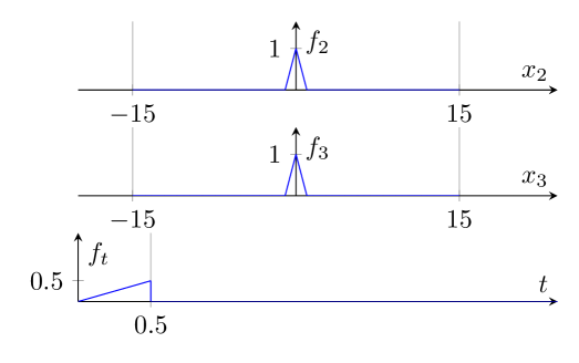
Fig. 1: Plot of the factor functions of the excitation signal

Thus the excitation signal acts in $x_{3}$-direction. We have taken this approach for the excitation signal from [6]. The only difference is that their the wave is excited at four different locations. The damaged areas are of cylindrical shape with the axis in thickness direction $x_{1}$ and a square as base with side length equal to one. There were three scenarios

• One damaged area approximately in the center of the plate at $(-1.5,1.5)$ (Scenario A)

• Two damaged areas, one of them nearer to to center of the plate at $(5.5,5.5)$, the other nearer to one edge of the plate at $(-1.5,-10.5)$ (Scenario B)

• Two damaged areas, both relatively close to the center of the plate at $(-1.5,-4.5)$ and $(5.5,5.5)$ (Scenario C)

We also stated the center of the square representing the respective damage area. The three damage scenarios are plotted in figure 2.

Fig. 2: The three damage scenarios. The black squares indicate the damage areas.

Let be $(\varphi_{r})_{r=1,...,L}$ the Lagrangian basis of the Galerkin space of the chosen Finite Element discretization. Then every basis function is at exactly one node equal to $1$ and at all other ones $0$. According to [6] we choose a basis element confined to the boundary of the plate as weighting function for every sensor of the observation operator. It follows that the observation matrix $W$ has the structure of a diagonal matrix multiplied with the boundary matrix $M_{\partial\Omega}$, where $(M_{\partial\Omega})_{rs}=\langle\varphi_{r},\varphi_{s}\rangle_{L^{2}(\partial\Omega,\mathbb{R}^{3})}$ with $r,s=1,...,L$ if $(\varphi_{r})_{r=1,...,L}$ is the Lagrangian basis. In this way for the description of the observation operator it is sufficient to indicate the nodes, which are associated with a basis element that is at the same time a weighting function.
The relaxation parameter $\omega$ was in all examples set to $10.0$. The value of the displacement $u_{S}$ is estimated experimentally by solving the problem for a given coefficient matrix $\alpha\in\mathbb{R}^{31\times 31}$. To interpret the results we plot the coefficient matrix, where several colors represent different values of the single entries of the coefficient matrix.
For our experiments we assumed initially to have complete data. In a first experiment we have computed 50 Iterations of the attenuated Landweber method for all three damage scenarios. The results are presented in figure 3.

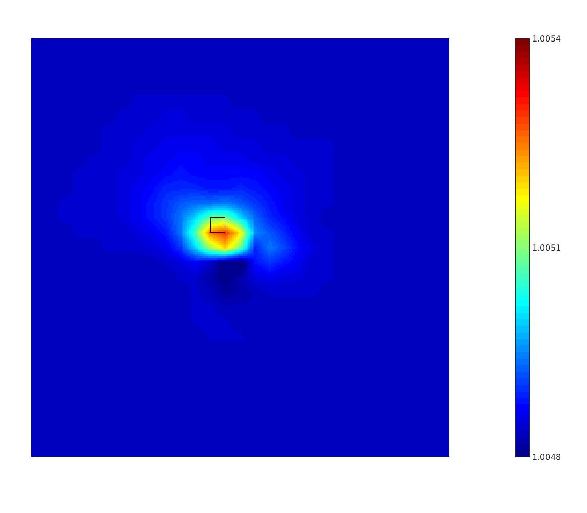
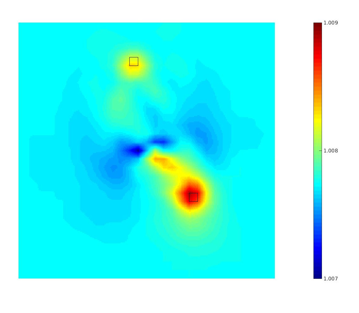
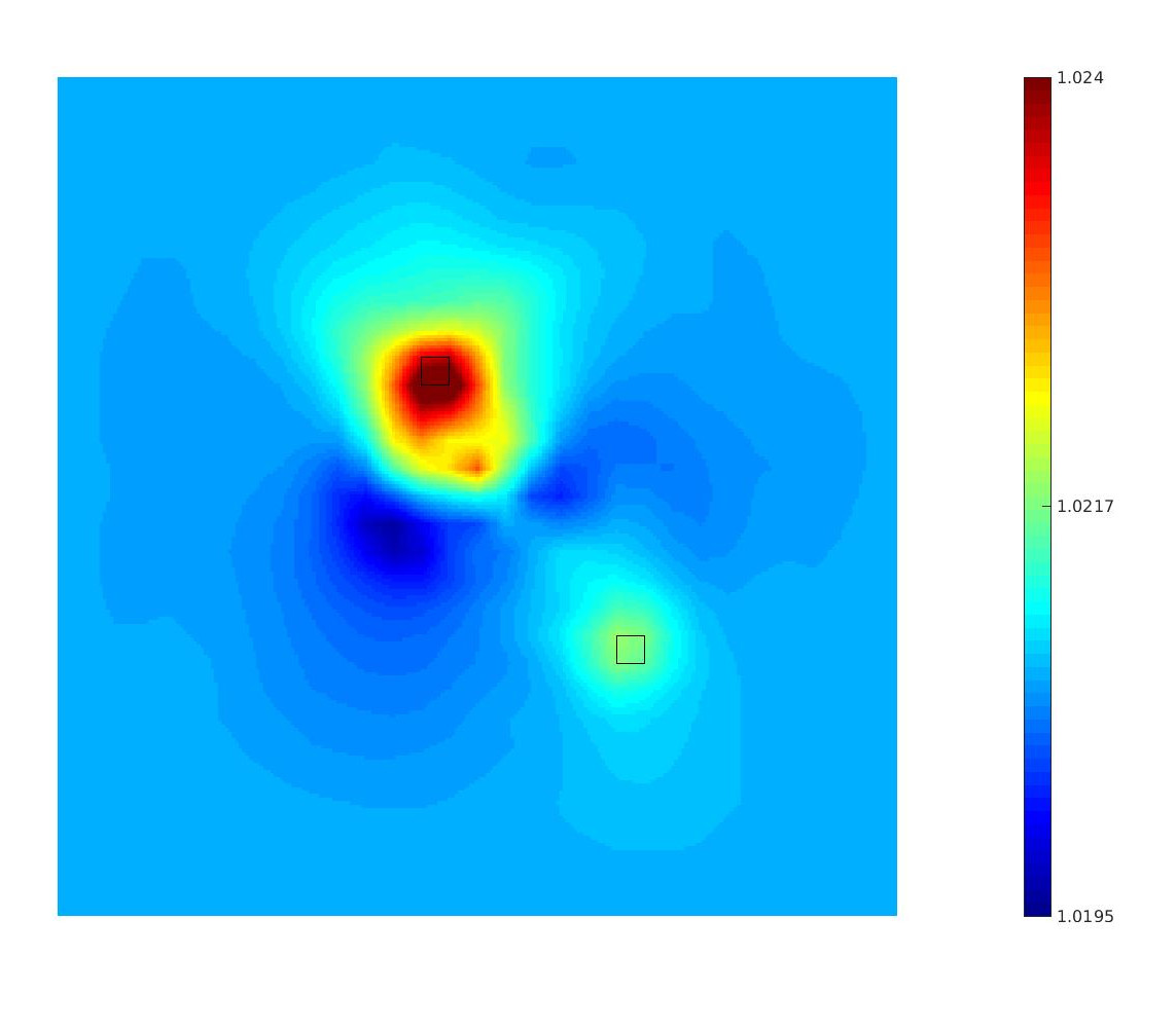
Fig. 3: The results of experiment 1 with damage scenarios A, B and C from left to right.

We see that our method can detect and localize the given damages. Regarding the damage scenarios B and C and therefore in case of two damaged areas it can be seen that there are artifacts between the center of the plate and the damaged area nearer to the center. One might suspect that the artifacts arise due to reflecions from the first damaged area meeting by the wave. To emphasize that we consider two damage scenarios with two damage areas.
In a second experiment we want to see how the results of the algorithm change in case of noisy data. For that purpose we add a random vector to the input data $\tilde{u}$ to get the noisy data $u^{\delta}$ with

$$\frac{\|U^{\delta}-\tilde{U}\|_{L^{2}(0,T;{\mathbb{R}}^{L})}}{\|\tilde{U}\|_{L^{2}(0,T;{\mathbb{R}}^{L})}}=\delta.$$

Here we use the representations $u^{\delta}(t_{j})=\sum_{r=1}^{L}U^{\delta}_{r}(t_{j})\varphi_{r}$ and $\tilde{u}(t_{j})=\sum_{r=1}^{L}\tilde{U}^{\delta}_{r}(t_{j})\varphi_{r}$ at the time points $t_{j}=jT/m$ for all $j=0,...,m$ (see Section 3). For our calculations we use different values up to 1 for $\delta$. In figure 4 one can see the difference between $\tilde{u}$ and $u^{\delta}$ for $\delta=1$ at time $t=108\mu\mbox{s}$.

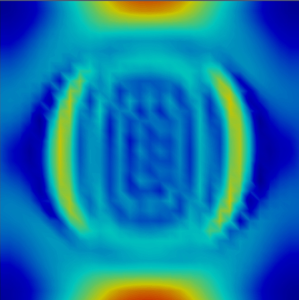
Fig. 4: The difference between exact and noisy input data with $\delta=1$. The displacement field corresponds to damage scenario A taken at time $t=108\mu\mbox{s}$. The coloring corresponds to the norm of the displacement field.

The result of experiment 2 is given in Figure 5 and proves the stability of the algorithm with respect to noise.

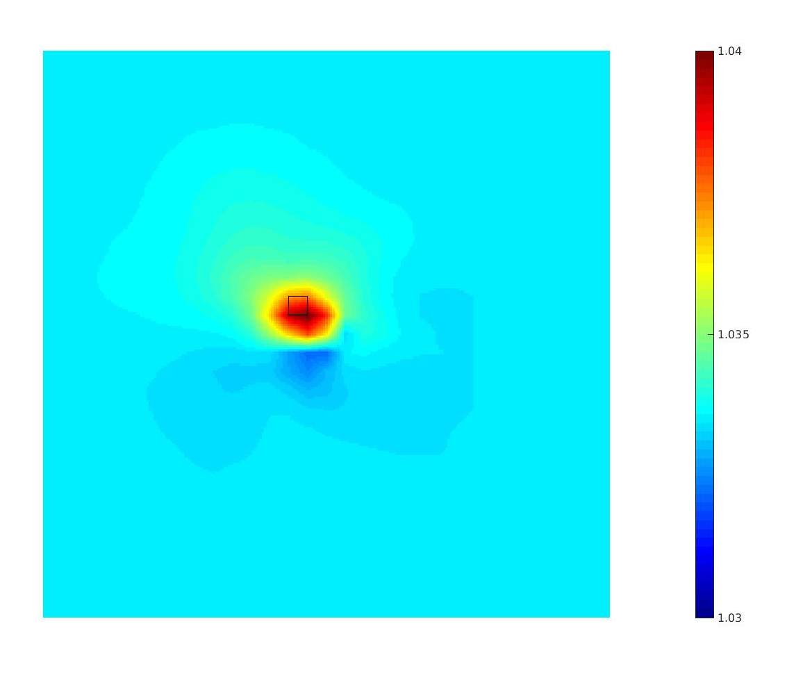
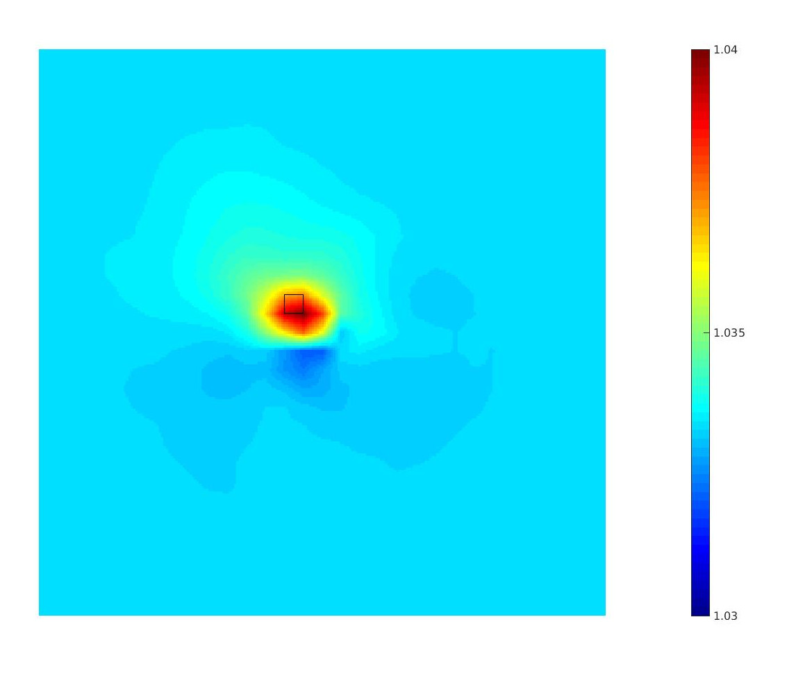
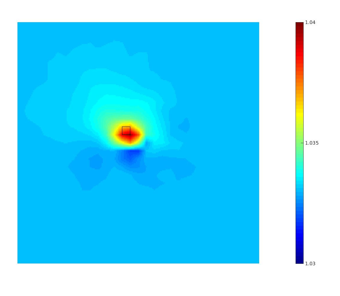
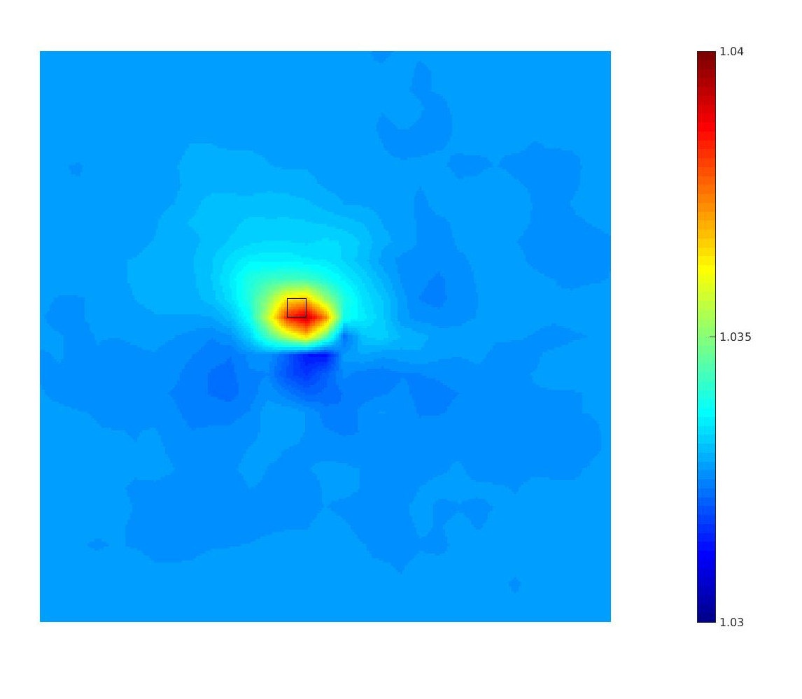
Fig. 5: The results of experiment 2. In every picture we considered damage scenario A. From top row left to bottom row right we have noise levels of $\delta=0$, $0.2$, $0.5$ and $1$.

In a third experiment we consider in contrast to the first two ones incomplete data. Therefore we use as input data the displacement field $\tilde{y}=\mathcal{Q}\tilde{u}$ with the observation operator $\mathcal{Q}$. In the experiment we computed the solution with two observation operators where the sensors are attached in parallel to the four edges of the plate on both sides of the plate. For the observation operator R57d there are $57$ sensors at every edge and so all in all $448$ at the whole plate and for the other one called R8d we have $8$ sensors at every edge and so $56$ sensors at th whole plate. The advantage of the usage of two different observation operators, where the sensors are attached in the same way, is that we can see, how the number of sensors influences the result of the experiment. In figure 6 we can see the result after $25$ iterations. It is obviously that indeed the damage is localized in both cases, but a higher number of sensors yields a better result. Using the observation operator R8d we have more artifacts and a smaller domain such that the localized damage is less visible compared to R57d.

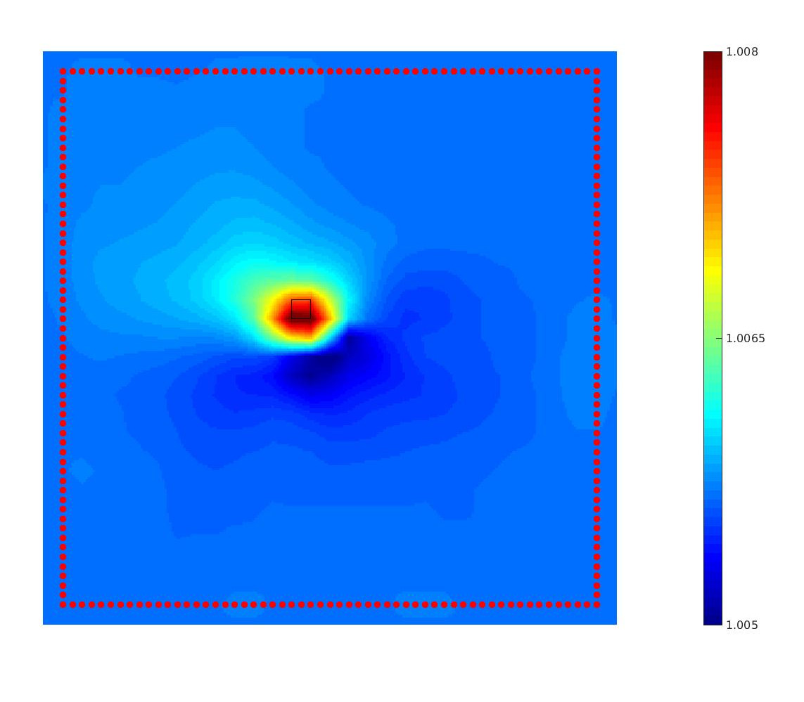
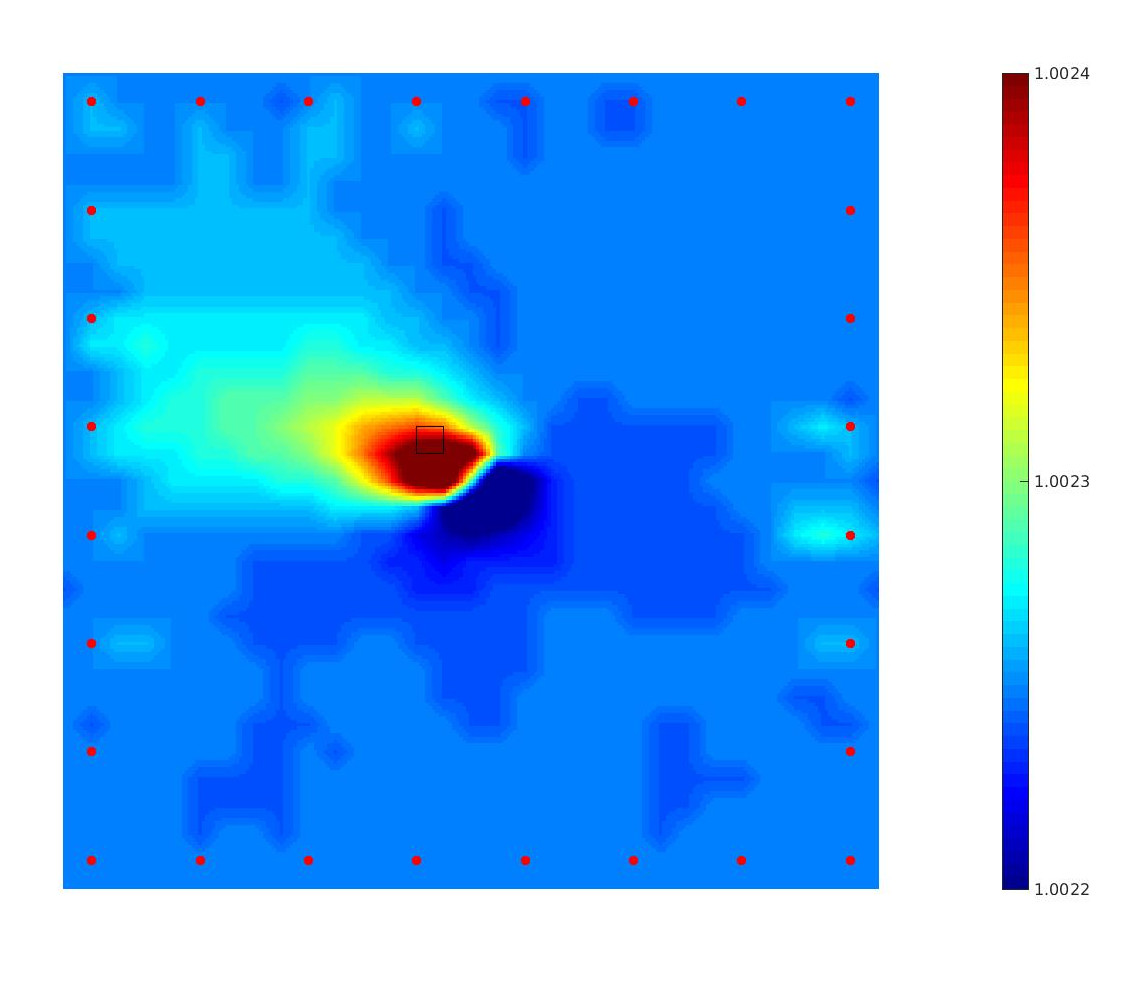
Fig. 6: The results of experiment 3. In both pictures we considered damage scenario A with observation operator R57d (left side) and R8d (right side). The sensors are marked by red dots.

6 Conclusion

In this article we proposed a method to detect defects in hyperelastic materials from full knowledge of the displacement field as well as sensor measurements acquired at the surface of the structure by solving a nonlinear inverse problem. The key idea is that we can represent the stored energy function of the hyperelastic material as a conic combination of suitable functions. Identifying these coefficients leads to the localization of defects in the structure. The arising inverse problem is highly nonlinear and ill-posed. In this article we solve the problem using the attenuated Landweber method. Therefore each iteration involves the solution of the nonlinear direct problem and the linear adjoint problem. The developed solver for the direct problem is also used to produce synthetic data. Numerical experiments showed a good performance in both cases of input data. We demonstrated that the method is also stable using noisy data. In addition it was proven that the considered identification problem fulfills the local tangential cone condition and hence that the attenuated Landweber method converges in the case of full knowledge of the displacement field to a solution of the inverse problem.

The given results show that the developed method present great space for future research. A next step in view of developing an autonomous, sensor based structural health monitoring system could be the verification of the method with real measurements at piezo sensors. Further research has to be done with respect to improve the efficiency of the method, since the Landweber method converges slowly. At the same time a finer discretization in time and space would be desirable but is out of reach because of the tremendous computing time. In that sense model reduction methods or sequential subspace optimization techniques (cf. [26, 30]) could be suitable remedies in near future. Furthermore it might be interesting to extend the numerical considerations to curved structures such as shells as they are applied in aircraft construction.

References

[1]D. D. Bainov and P. S. Simeonov, Integral Inequalities and
Applications, Mathematics and its Applications, vol. 57 of East European
series, Kluwer Academic Publishers, Dordrecht, 1992.
[2]G. Bal, C. Bellis, S. Imperiale, and F. Monard, Reconstruction of
constitutive parameters in isotropic linear elasticity from noisy full-field
measurements, Inverse Problems, 30 (2014), p. 125004.
[3]G. Bal, F. Monard, and G. Uhlmann, Reconstruction of a fully
anisotropic elasticity tensor from knowledge of displacement fields, SIAM J.
Appl. Math., 75 (2015), pp. 2214––2231.
[4]J. M. Ball, Convexity conditions and existence theorems in nonlinear
elasticity, Archive for Rational Mechanics and Analysis, 63 (1977),
pp. 337–403.
[5]W. Bangerth, R. Hartmann, and G. Kanschat, deal.II – A General
Purpose Object Oriented Finite Element Library, ACM Trans. Math. Softw., 33
(2007), pp. 24/1–24/27.
[6]F. Binder, F. Schöpfer, and T. Schuster, Defect localization in
fibre-reinforced composites by computing external volume forces from surface
sensor measurements, Inverse Problems, 31 (2015).
ID 025006, 22pp.
[7]C. Boehm and M. Ulbrich, A semismooth newton-cg method for
constrained parameter identification in seismic tomography, SIAM Journal on
Scientific Computing, 37 (2015), pp. S334–S364.
[8]M. Bonnet and A. Constantinescu, Inverse problems in elasticity,
Inverse Problems, 21 (2005), pp. R1–R50.
[9]L. Bourgeois, F. Le Louër, and E. Lunéville, On the use of
Lamb modes in the linear sampling method for elastic waveguides, Inverse
Problems, 27 (2011).
ID 055001, 27pp.
[10]L. Bourgeois and E. Lunéville, On the use of the linear sampling
method to identify cracks in elastic waveguides, Inverse Problems, 28
(2012).
ID 105011, 18pp.
[11]P. G. Ciarlet, Mathematical Elasticity, vol. 20 of Studies in
Mathematics and its Applications, North Holland, Amsterdam, 1994.
[12]D. Colton and A. Kirsch, A simple method for solving inverse
scattering problems in the resonance region, Inverse Problems, 12 (1996),
pp. 383–393.
[13]P. Deuflhard, H. W. Engl, and O. Scherzer, A convergence analysis of
iterative methods for the solution of nonlinear ill-posed problems under
affinely invariant conditions, Inverse Problems, 14 (1998), pp. 1081–1106.
[14]H. W. Engl, M. Hanke, and A. Neubauer, Regularization of Inverse
Problems, Mathematics and Its Applications, Kluwer Academic Publishers,
Dordrecht, 1996.
[15]V. Giurgiutiu, Structural Health Monitoring with Piezoelectric Wafer
Active Sensors, Academic Press, 2008.
[16]M. Hanke, A. Neubauer, and O. Scherzer, A convergence analysis of
the landweber iteration for nonlinear ill-posed problems, Numerische
Mathematik, 72 (1995), pp. 21–37.
[17]G. A. Holzapfel, Nonlinear Solid Mechanics, Wiley, 2000.
[18]D. Jiang, Y. Liu, and M. Yamamoto, Theoretical stability and
numerical reconstruction for an inverse source problem for hyperbolic
equations, arXiv preprint arXiv:1509.04453, (2015).
[19]B. Kaltenbacher and A. Lorenzi, A uniqueness result for a nonlinear
hyperbolic equation, Applicable Analysis, 86 (2007), pp. 1397–1427.
[20]B. Kaltenbacher, A. Neubauer, and O. Scherzer, Iterative
Regularization Methods for Nonlinear Ill-Posed Problems, Radon
series on computational and applied mathematics, Walter de Gruyter, 2008.
[21]A. Kirsch and A. Rieder, On the linearization of operators related
to the full waveform inversion in seismology, Math. Meth. Appl. Sci., 37
(2014), pp. 2995–3007.
[22]A. Lechleiter and J. W. Schlasche, Identifying lamé parameters
from time-dependent elastic wave measurements, Inverse Problems in Science
and Engineering, 25 (2017), pp. 2–26.
[23]J. E. Marsden and T. J. R. Hughes, Mathematical Foundations of
Elasticity, Dover Publications, New York, 1983.
[24]N. Rauter and R. Lammering, Investigation of the Higher Harmonic
Lamb Wave Generation in Hyperelastic Isotropic Material, Physics
Procedia, 70 (2015), pp. 309–313.
[25]O. Scherzer, An iterative multi level algorithm for solving
nonlinear ill–posed problems, Numerische Mathematik, 80 (1998),
pp. 579–600.
[26]F. Schöpfer and T. Schuster, Fast regularizing sequential
subspace optimization in Banach spaces, Inverse Problems, 25 (2009),
pp. 1–22.
[27]T. Schuster and A. Wöstehoff, On the identifiability of the stored
energy function of hyperelastic materials from sensor data at the boundary,
Inverse Problems, 30 (2014).
ID 105002, 26pp.
[28]J. Seydel and T. Schuster, On the linearization of identifying the
stored energy function of a hyperelastic material from full knowledge of the
displacement field, Math. Meth. Appl. Sci., 40 (2016), pp. 183–204.
[29]J. C. Simo and N. Tarnow, The discrete energy-momentum method.
conserving algorithms for nonlinear elastodynamics, Z. Angew. Math. Phys.,
43 (1992), pp. 757–792.
[30]A. Wald and T. Schuster, Sequential subspace optimization for
nonlinear inverse problems, Journal of Inverse and Ill-Posed Problems, 25
(2017), pp. 99–118.
[31]A. Wöstehoff and T. Schuster, Uniqueness and stability result for
Cauchy’s equation of motion for a certain class of hyperelastic materials,
Applicable Analysis, 94 (2015), pp. 1561–1593.