Hydrodynamic limit and viscosity solutions for a 2D growth process in the anisotropic KPZ class

Abstract.

We study a $(2+1)$-dimensional stochastic interface growth model, that is believed to belong to the so-called Anisotropic KPZ (AKPZ) universality class [4, 5]. It can be seen either as a two-dimensional interacting particle process with drift, that generalizes the one-dimensional Hammersley process [1, 22], or as an irreversible dynamics of lozenge tilings of the plane [4, 27]. Our main result is a hydrodynamic limit: the interface height profile converges, after a hyperbolic scaling of space and time, to the solution of a non-linear first order PDE of Hamilton-Jacobi type with non-convex Hamiltonian (non-convexity of the Hamiltonian is a distinguishing feature of the AKPZ class). We prove the result in two situations: (i) for smooth initial profiles and times smaller than the time $T_{shock}$ when singularities (shocks) appear or (ii) for all times, including $t>T_{shock}$, if the initial profile is convex. In the latter case, the height profile converges to the viscosity solution of the PDE. As an important ingredient, we introduce a Harris-type graphical construction for the process.

1. Introduction

The study of random interface growth models witnessed a spectacular progress recently, especially in relation with the so-called KPZ equation, cf. e.g. [12, 8] for recent reviews. The $d$-dimensional discrete interface is modeled by the graph of a function $h$ from $\mathbb{Z}^{d}$ (or some other $d-$dimensional lattice) to $\mathbb{Z}$. The dynamics is an irreversible Markov chain and the asymmetry of the transition rates by which the interface height locally increases or decreases produces a non-trivial and slope-dependent average drift. Among the most interesting and challenging questions are the problem of obtaining hydrodynamic limits [17, 25] – the convergence of the height function, when space and time are rescaled hyperbolically, to a first-order PDE – and of understanding the large-scale behavior of space-time correlations of the height fluctuation process, be it in the stationary state or around the typical macroscopic profile described by the hydrodynamic limit equation. Most of the known rigorous results, as far as both hydrodynamic limits and fluctuations are concerned, have been proven for one-dimensional models, often in cases where the invariant measures of interface gradients are of i.i.d. type. Much less is known for $d$-dimensional models, $d\geq 2$ (see Section 1.1 for a brief overview of the literature).

When $d=2$, growth models are conjectured to fall into two distinct universality classes, called the “Isotropic” and “Anisotropic” KPZ classes [28]. (For simplicity we will refer to these two classes as KPZ and AKPZ, respectively). For models in the KPZ class, height fluctuations are believed (and numerically observed [26]) to grow as a non-trivial power $t^{z}$ of time $t$, as $t\to\infty$. On the other hand, for models in the AKPZ class, height fluctuations are believed to converge asymptotically in the scaling limit to the solution of a stochastic heat equation with additive noise; in particular, the variance of height fluctuations should grow like $\log t$. Conjecturally [28], the universality class a particular growth model falls into is determined by the convexity properties of the function $v(\rho)$ that gives the average interface drift in the translation-invariant stationary state with slope $\rho$. Namely, it is predicted that if the signature of the Hessian of $v(\cdot)$ is either $(+,+)$ or $(-,-)$, then the model falls into the isotropic KPZ class. The AKPZ class is instead relevant when the signature is $(+,-)$ (the borderline cases, where one eigenvalue is zero and the second is not, is also conjectured to belong to the AKPZ class).

In this work, we analyze a two-dimensional growth model in the AKPZ class, that was originally introduced in [4, 5] and later studied in [27]. There are various equivalent ways to view this process. One of them is to see it as a dynamics on lozenge tilings of the plane: the interface is then the graph of the height function canonically associated to the tiling (see Fig. 4). Another useful viewpoint is to interpret it as a driven, interacting system of interlaced particles that evolve on a two-dimensional lattice via long-range jumps. Suitable sections of the particle system behave like mutually interacting one-dimensional, discrete, Hammersley-Aldous-Diaconis processes. In this sense, our growth process is a two-dimensional generalization of the Hammersley-Aldous-Diaconis process [1, 22, 11]. Yet another viewpoint is taken in [4, 5], where the process is seen as a two-dimensional totally asymmetric driven system of interacting particles that perform only jumps of size $1$ but can “push” other particles arbitrarily far away.

The main result of the present work is a hydrodynamic limit: when space and time are rescaled hyperbolically ($x=\xi L,t=\tau L$ and $L\to\infty$), the height function rescaled by $1/L$ converges in probability to the solution of a first-order non-linear PDE of Hamilton-Jacobi type. Such equations are known to have singularities at a finite time $T_{shock}$: their gradient develops discontinuities or shocks. Our hydrodynamic limit result is proven in two situations: either (i) for smooth initial profile and for times up to $T_{shock}$ (Theorem 3.5) or (ii) for all times, provided the initial profile is convex (Theorem 3.6). In the latter case, the relevant weak solution of the PDE to which the height profile converges is the so-called viscosity solution [9]. It is tempting to conjecture that convergence to the viscosity solution of the PDE holds for all times also for non-convex initial data.

The PDE describing the hydrodynamic limit is of the Hamilton-Jacobi form

$$\partial_{\tau}\phi(\xi,\tau)+v(\nabla\phi(\xi,\tau))=0,$$ (1.1)

where the “Hamiltonian” (or rather “drift”) function $v(\cdot)$ is an explicit function (cf. (3.3)) whose Hessian has a $(+,-)$ signature for every slope. As we mentioned above, this is a distinguishing feature of the AKPZ universality class but it is also a remarkable source of difficulties, since the solution of (1.1) cannot be expressed by a Hopf-Lax type formula. At the probabilistic level, lack of convexity prevents to prove the hydrodynamic limit via simple super-additivity arguments. More comments on these points can be found in Section 1.1.

Let us mention two previous results on our growth model, that are relevant for the discussion here. First, in [4] the hydrodynamic limit was proven for a special initial condition, where particles are perfectly packed in a certain wedge-shaped region of the lattice. The special features of such initial conditions allow for the application of “integrable probability methods” and in particular for the exact computation, in terms of sums of determinants, of the average particle currents integrated in time. While the same methods may allow to analyze other “integrable” initial conditions (and also more general, but still integrable, two-dimensional random growth models, see e.g. [3, Sec. 3.3]), they are not robust enough to yield “generic” results, where the initial microscopic configuration is just assumed to approximate a macroscopic profile satisfying some smoothness assumptions. The methods we use here are of entirely different nature with respect to those of [4] and we do not rely on the integrable structure of the dynamics. Let us also observe that the initial condition chosen in [4] is such that shocks do not appear: characteristic lines of the PDE never cross.

Secondly, a special feature of this growth process is that its stationary measures, labelled by the average slope, are known [27]: they coincide with the translation invariant, ergodic Gibbs measures on lozenge tilings, obtained as limits of uniform distributions on the torus with fixed proportions of lozenges [16]. It is the knowledge of the stationary states that allows to obtain an explicit expression for the drift function $v(\cdot)$.

1.1. Comments on the result and on related literature

Hydrodynamic limit results for interface growth models in dimension $d\geq 2$ are rare; here we briefly review the more relevant for us, trying to emphasize the differences with our case. (For $d=1$ the literature is much more vast and we refer for instance to the introduction of [19] for a discussion of known results and a list of references). In [19], a class of $d$-dimensional growth models, called v-exclusion processes there, was studied: they enjoy a property called “strong monotonicity”, that is stronger than the stochastic domination or “attractity” property discussed e.g. in Section 5.2 of the present work. The proof of the hydrodynamic limit in [19] heavily relies on super-additivity arguments and the drift function $v(\cdot)$ in the limit PDE is automatically convex, so that in particular these models necessarily fall into the isotropic KPZ class. Similar ideas were used earlier [23] to obtain the hydrodynamic limit for a $d$-dimensional ballistic deposition model: again, the height function converges to the Hopf-Lax solution of a Hamilton-Jacobi equation with convex drift function. In our context, it is relevant to mention also the work [24], that obtains the hydrodynamic limit for a $d$-dimensional generalization of the Hammersley-Aldous-Diaconis process, though such generalization is quite different, even for $d=2$, from the $2$-dimensional one we study here. Notably, once again the drift function in [24] turns out to be (strictly) convex and, in contrast with [19, 23], it is fully explicit. Also in [24], the proof of convergence to the Hopf-Lax solution of the PDE uses super-additivity.

Another very interesting work is [20]: the growth models studied there do not satisfy strongly monotonicity. For dimension $d\geq 2$, however, the hydrodynamic limit obtained there is weak in the sense that it is not known that the drift function $v(\cdot)$ is non-random (i.e., the height function could converge in the scaling limit to the solution of a random first order Hamilton-Jacobi equation).

The Markov chain we study in the present work is rather different from those just mentioned. For one thing, it does not satisfy strong monotonicity, super-additive arguments do not work and, as we already noted, the drift function $v(\cdot)$ in (1.1) turns out to have no definite convexity or concavity. What comes to rescue is the knowledge of the stationary measures, that allows to compute $v(\cdot)$. Lack of convexity of $v(\cdot)$ induces serious analytic problems in the analysis of the PDE. Notably, we are not aware of any variational formula of the Hopf-Lax type expressing its solution, for general initial condition. This is one of the main reasons why we cannot prove convergence to the hydrodynamic limit for general initial profiles and for times $t>T_{shock}$. A Hopf-type variational formula is however available when the initial datum is convex or concave [2], and this is strongly used in the proof of Theorem 3.6 below.

Let us conclude this introduction with a few more comments on the peculiar technical difficulties one encounters in the proof of the hydrodynamic limit for our growth process. An important ingredient in the methods of [20], that is a key step to obtain a tightness property in Skorohod space for the height function process, is that, uniformly with respect to the initial condition, the height at a given point can grow at most linearly in time. This is definitely false for our model. In fact, the average speed of growth is larger and larger as the particles are more and more mutually spaced. This can be seen, at the macroscopic level, by the fact that the function $v(\cdot)$ in (3.3) diverges as $\rho_{1}+\rho_{2}$ tends to $1$ (as we will see, this corresponds exactly to the situation where particle spacings diverge). One might hope that, if particle spacings are tight in the initial condition, then the same holds at all later times. For instance, a stochastic domination property of the following type would be very helpful: given two configurations such that the former has larger particle spacings than the latter, the evolutions with the two initial conditions can be coupled in a way that the same property holds at all later times. In fact, a property of this type is valid for the one-dimensional Hammersley-Aldous-Diaconis process [22, Sec. 6], but unfortunately it seems to fail for our two-dimensional model. The estimates on “speed of propagation of information” and the “localization procedure” introduced in Section 5, as well as the iterative procedure of Sections 6.2 and 7, are devised precisely to overcome these difficulties. Finally, let us emphasize that an important tool for our proof, as was the case for the Hammersley-Aldous-Diaconis processes in [22], is a formulation of the growth process in terms of a suitable graphical construction.

Organization of the article

In Section 2 we define the state space of the interacting particle model and the associated height function; moreover, we introduce the growth process via a graphical construction and we state some of its basic properties (Proposition 2.8, that is proven in Section 4). In Section 3 we state our main result: the hydrodynamic limit for the height function (Theorems 3.5 and 3.6). In Section 5 we prove two crucial properties of the dynamics: monotonicity and a bound on the speed of propagation of information. Finally, Theorems 3.5 and 3.6 are proved in Sections 6 and 7 respectively.

2. Model

2.1. Configuration space and informal description of the dynamics

The lattice where particles live consists of an infinite collection of horizontal lines, labeled by an index $\ell\in\mathbb{Z}$. Each line contains an infinite collection of particles, each having a label $(p,\ell)$, $p\in\mathbb{Z}$. See Figure 1. Horizontal particle positions $z_{(p,\ell)}$ are discrete and

$$z_{(p,\ell)}\in\mathbb{Z}+(\ell\!\!\!\!\mod 2)/2:$$

on lines with index $\ell\in 2\mathbb{Z}$ one has $z_{(p,\ell)}\in\mathbb{Z}$, while on lines with index $\ell\in 2\mathbb{Z}+1$ one has $z_{(p,\ell)}\in\mathbb{Z}+1/2$ (the reason for this choice is that it will be convenient that no two particles in neighboring lines have the same horizontal position).

Moreover, particle positions satisfy a number of constraints:

Definition 2.1.

We let $\Omega$ be the set of particle configurations $\eta$ satisfying the following properties:

1. no two particles in the same line $\ell$ have the same position $z_{(p,\ell)}$. We can then label particles in each line in such a way that $z_{(p,\ell)}<z_{(p+1,\ell)}$. Labels should be seen as attached to particles, and they will not change along the dynamics.

2. particles are interlaced in the following sense: for every $\ell$ and $p$, there exists a unique $p^{\prime}\in\mathbb{Z}$ such that $z_{(p,\ell)}<z_{(p^{\prime},\ell+1)}<z_{(p+1,\ell)}$ (and, as a consequence, also a unique $p^{\prime\prime}\in\mathbb{Z}$ such that $z_{(p,\ell)}<z_{(p^{\prime\prime},\ell-1)}<z_{(p+1,\ell)}$). Without loss of generality, we will assume that $p^{\prime}=p$ (and therefore $p^{\prime\prime}=p+1$). This can always be achieved by deciding which particle is labeled $0$ on each line. Also, by convention, we establish that the particle labeled $(0,0)$ is the left-most one on line $\ell=0$, with non-negative horizontal coordinate.

3. for every $\ell$ one has

   $$\lim_{p\to-\infty}\frac{z_{(p,\ell)}}{p^{2}}=0.$$ (2.1)

Note that if condition (2.1) holds for $\ell=0$ it holds for every $\ell$.

Here we give an informal description of the dynamics. A more rigorous version is given in Section 2.3. The property (3) in Definition 2.1 will ensure that the dynamics is well-defined.

Given the particle labelled $(p,\ell)$, we denote $I_{(p,\ell)}=\{(p-1,\ell+1),(p,\ell-1)\}$, see Fig. 1. Note that these are simply the labels of the two particles directly to the left of $(p,\ell)$ on lines $\ell+1$ and $\ell-1$.

Figure 1. The set $I_{(p,\ell)}$ comprises the particle labels of the two particles in the dotted region. The particle $(p,\ell)$ can jump to the position marked by the cross (and does so with rate $1$) but cannot jump to the position marked by a square, because it would have to overcome the particles in $I_{(p,\ell)}$.

To every pair $(\ell,z)$ with $\ell\in\mathbb{Z}$ and $z\in\mathbb{Z}+(\ell\!\!\mod 2)/2$ we associate an i.i.d. Poisson clock of rate $1$. When the clock labeled $(\ell,z)$ rings, then:

• if position $(\ell,z)$ is occupied, i.e. if there is a particle on line $\ell$ with horizontal position $z$, then nothing happens;

• if position $(\ell,z)$ is free, let $(p,\ell)$ denote the label of the left-most particle on line $\ell$, with $z_{(p,\ell)}>z$. If both particles in $I_{(p,\ell)}$ have horizontal position smaller than $z$, then particle $(p,\ell)$ is moved to position $(\ell,z)$; otherwise, nothing happens.

The second point can be described more compactly as follows: is position $(\ell,z)$ is free, then particle $(p,\ell)$ is moved to position $(\ell,z)$ if and only if the new configuration is still in $\Omega$, i.e. if the interlacement constraints are still satisfied.

Remark 2.2.

Recall the definition [11] of the one-dimensional (discrete) Hammersley-Aldous-Diaconis (HAD) process: on each site $x\in\mathbb{Z}$ there is at most one particle; each particle jumps with rate $1$ to any position that is at the same time to its left and to the right the next particle. Going back to our two-dimensional interacting particle system, we see that particles on each line $\ell$ follow a HAD process, except that particle jumps can be prevented by the interlacing constraints with particles in lines $\ell\pm 1$. This induces non-trivial correlations between the processes on different lines. As discussed in Section 5.1, the invariant measures of the two-dimensional dynamics restricted to any line $\ell$ are very different from the (i.i.d. Bernoulli) invariant measures of the HAD process.

2.2. Height function

To each configuration $\eta\in\Omega$ we associate an integer-valued height function $h_{\eta}$. We first give the definition, then we motivate it via the bijection between particle configurations and lozenge tilings of the plane.

First of all let us remark that the graph $G$ whose vertices are all the possible particle positions $(\ell,z),\ell\in\mathbb{Z},z\in\mathbb{Z}+(\ell\!\!\mod 2)/2$ and where the neighbors of $(\ell,z)$ are the four vertices $(\ell\pm 1,z\pm 1/2)$ can be identified with $\mathbb{Z}^{2}$, rotated by $\pi/4$ and suitably rescaled, see Figure 2.

Figure 2. The lattice $G$ (dotted, with black vertices that are possible particle positions $(\ell,z)$, with $z\in\mathbb{Z}+(\ell\!\!\mod 2)/2$), the lattice $G^{*}$ (bold, with white vertices) and the two coordinate vectors $e_{1},e_{2}$. The origin of $G^{*}$ (encircled) is the point of horizontal coordinate $z=-1/2$ on line $\ell=0$.

The height function $h_{\eta}$ is defined on the dual graph $G^{*}$, that is just obtained by shifting $G$ horizontally by $1/2$, see Figure 2. In other words, on each line $\ell$, the height function is defined at horizontal coordinates $n\in\mathbb{Z}+((\ell+1)\!\!\mod 2)/2$.

There is a natural and convenient choice of coordinates on $G^{*}$:

Definition 2.3 (Coordinates on $G^{*}$).

The point of $G^{*}$ of horizontal coordinate $-1/2$ of the line labeled $\ell=0$ is assigned the coordinates $(x_{1},x_{2})=(0,0)$. The unit vector $e_{1}$ (resp. $e_{2}$) is the vector from $(0,0)$ to the point of horizontal coordinate $0$ on the line labeled $\ell=-1$ (resp. $\ell=+1$), see Figure 2. With this convention, the vertex of $G^{*}$ labeled $(x_{1},x_{2})$ is on line

$$\bar{\ell}(x)=x_{2}-x_{1}$$ (2.2)

and has horizontal coordinate

$$\bar{z}(x)=(x_{1}+x_{2}-1)/2.$$ (2.3)

We can now define the height function $h_{\eta}$:

Definition 2.4 (Height function).

Given a configuration $\eta\in\Omega$, its height function $h_{\eta}$ is an integer-valued function defined on $G^{*}$. We fix $h_{\eta}(0,0)$ to some constant (e.g. to zero) and then it is enough to define the gradients $h_{\eta}(x_{1}+1,x_{2})-h_{\eta}(x_{1},x_{2})$ and $h_{\eta}(x_{2},x_{2}+1)-h_{\eta}(x_{1},x_{2})$ to fix $h_{\eta}$ unambiguously.

Given $(x_{1},x_{2})\in G^{*}$, let $p$ (resp. $p+1$) be the index of the rightmost (resp. leftmost) particle on line $\ell=x_{2}-x_{1}$ that is to the left (resp. to the right) of $(x_{1},x_{2})$. Recall that particle $p$ of line $\ell+1$ satisfies $z_{p,\ell}<z_{p,\ell+1}<z_{p+1,\ell}$. We establish that

$$\Delta_{2}h_{\eta}(x_{1},x_{2}):=h_{\eta}(x_{1},x_{2}+1)-h_{\eta}(x_{1},x_{2})\\ =\left\{\begin{array}[]{ccc}0&\text{if}&(x_{1},x_{2}+1)\text{ is to the right of particle }(p,\ell+1)\\ 1&\text{if}&(x_{1},x_{2}+1)\text{ is to the left of particle }(p,\ell+1)\end{array}\right.$$ (2.4)

and similarly

$$\Delta_{1}h_{\eta}(x_{1},x_{2}):=h_{\eta}(x_{1}+1,x_{2})-h_{\eta}(x_{1},x_{2})\\ =\left\{\begin{array}[]{ccc}0&\text{if}&(x_{1}+1,x_{2})\text{ is to the right of particle }(p+1,\ell-1)\\ 1&\text{if}&(x_{1}+1,x_{2})\text{ is to the left of particle }(p+1,\ell-1).\end{array}\right.$$ (2.5)

See Figure 3.

Figure 3. A portion of particle configuration and the corresponding height function. Particles (black dots) are on vertices of $G$ and the height is defined on vertices of $G^{*}$.

We leave it to the reader to check that

$$\Delta_{1}h_{\eta}(x_{1},x_{2})+\Delta_{2}h_{\eta}(x_{1}+1,x_{2})=\Delta_{2}h_{\eta}(x_{1},x_{2})+\Delta_{1}h_{\eta}(x_{1},x_{2}+1)\\ =h_{\eta}(x_{1}+1,x_{2}+1)-h_{\eta}(x_{1},x_{2})=\left\{\begin{array}[]{ll}0&\text{if $\exists$ particle between }(x_{1},x_{2})\text{ and }(x_{1}+1,x_{2}+1)\\ 1&\text{if $\nexists$ particle between }(x_{1},x_{2})\text{ and }(x_{1}+1,x_{2}+1).\end{array}\right.$$ (2.6)

The first equality in (2.6) implies that the sum of gradients of $h_{\eta}$ along any closed circuit is zero, so that the definition of $h_{\eta}$ is well-posed.

Let $\mathbb{T}\subset\mathbb{R}^{2}$ denote the closed triangle with vertices $(0,0),(1,0),(0,1)$ and $\stackrel{{\scriptstyle\circ}}{{\mathbb{T}}}$ be its interior. The following holds:

Lemma 2.5.

Let $A\subset\stackrel{{\scriptstyle\circ}}{{\mathbb{T}}}$. Let $\phi:\mathbb{R}^{2}\mapsto\mathbb{R}$ be a Lipschitz function satisfying $\nabla\phi(x)\in A$ for almost every $x\in\mathbb{R}^{2}$. There exists a sequence $\{\eta^{(L)}\}_{L\in\mathbb{N}}$ in $\Omega$ such that

$$|h_{\eta}(x)-L\phi(x/L)|\leq 1\quad\text{ for every }\quad x\in\mathbb{Z}^{2}.$$ (2.7)

The proof of Lemma 2.5 is given at the end of next section since it is more immediate after discussing the mapping between particle configurations and lozenge tilings.

The restriction $\nabla\phi(x)\in\mathbb{T}$ can be easily understood as follows. At the microscopic level, the interface gradients

$$h_{\eta}(x+(1,0))-h_{\eta}(x),\;h_{\eta}(x+(0,1))-h_{\eta}(x),\;h_{\eta}(x+(1,1))-h_{\eta}(x)$$ (2.8)

all belong to $\{0,1\}$. Therefore, any Lipschitz interface $\phi$ that can be approximated by a discrete one must verify $\partial_{x_{i}}\phi\in[0,1]$, as well as $\partial_{x_{1}}\phi+\partial_{x_{2}}\phi\in[0,1]$. This is exactly the condition $\nabla\phi\in\mathbb{T}$.

2.2.1. Height function and mapping to lozenge tilings

In order to understand the definition of height function given above, let us first of all recall that there is a bijection between interlaced particle configurations satisfying properties (1)-(2) of Definition 2.1 and lozenge tilings of the plane, as in Figure 4.

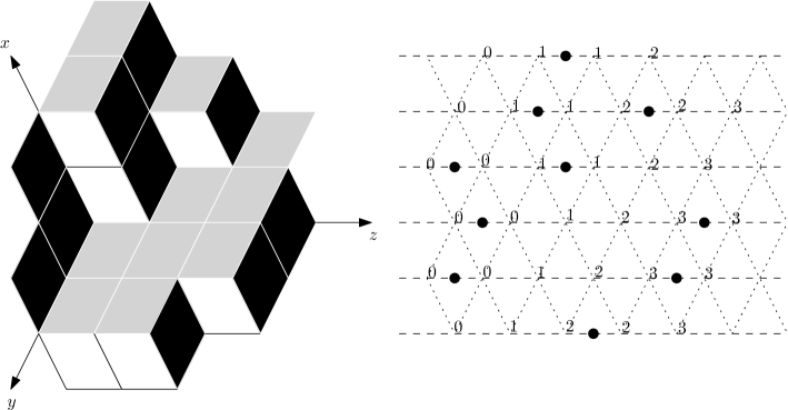
Figure 4. The bijection between lozenge tiling (or stepped interface) and particle configuration: vertical (black) lozenges correspond to particles (dots). The reader may check that the height function in the right drawing corresponds to the height in the $z$ direction, that is w.r.t. the $(x,y)$ plane, of the pile of cubes in the left drawing.

Particles correspond to vertical lozenges: the vertical coordinate of the central point of a vertical lozenge defines the line the particle is on, and its horizontal coordinate corresponds to the $z_{(p,\ell)}$ coordinate of the particle. Note that, if lengths are rescaled in such a way that lozenge sides are $1$, then horizontal positions of vertical lozenges are shifted by half-integers between neighboring lines (as is the case for particles). That horizontal positions of lozenges in neighboring lines satisfy the same interlacings as particle positions $z_{(p,\ell)}$, as well as the fact that the tiling-to-particle configuration mapping is a bijection, is well known and easy to understand from the picture.

Given a lozenge tiling as in Figure 4 and viewing it as the boundary of a stacking of unit cubes in $\mathbb{R}^{3}$, a natural definition of height function is to assign to each vertex of a lozenge the height (i.e. the $z$ coordinate) w.r.t. the $(x,y)$ plane of the point (in $\mathbb{R}^{3}$) in the corresponding unit cube. As a consequence, height is integer-valued and defined on points that are horizontally shifted $1/2$ w.r.t. centers of lozenges, i.e. on points of $G^{*}$. We leave to the reader to check that the height function as defined in the previous section precisely corresponds to the height of the stack of cubes w.r.t. the $(x,y)$ plane.

Proof of Lemma 2.5.

Define

$$h(x):=\lfloor L\phi(x/L)\rceil,\,x\in\mathbb{Z}.$$ (2.9)

We want first to prove that such function $h(\cdot)$ is the height function of some lozenge tiling. Given $x$, let

$$n_{1}(x)=h(x+(1,0))-h(x),\\ n_{2}(x)=h(x+(1,1))-h(x+(1,0),\\ n_{3}(x)=1-[h(x+(1,1))-h(x)].$$ (2.10)

By the assumption $\nabla\phi\in\mathbb{T}$, we see that $n_{i}(x)\in\{0,1\}$. Also, since $n_{1}(x)+n_{2}(x)+n_{3}(x)=1$, we have that necessarily two of them are $0$ and the third is $1$. Draw an edge between $x$ and $x+(1,0)$ (resp. between $x+(1,0)$ and $x+(1,1)$, resp. between $x$ and $x+(1,1)$) if $n_{1}(x)=0$ (resp. if $n_{2}(x)=0$, resp. if $n_{3}(x)=0$) and no edge otherwise. Therefore, we see that the set of edges defines a lozenge tiling of the plane (every elementary triangle $x,x+(1,0),x+(1,1)$ has two edges on the boundary of a lozenge and the third crosses a lozenge) and it is clear that $h$ is just the height function of the corresponding cube stacking.

To prove that $h(\cdot)$ in (2.9) is the height function of a particle configuration in $\Omega$ it remains to show that (2.1) is satisfied. Since $\nabla\phi\in A\subset\stackrel{{\scriptstyle\circ}}{{\mathbb{T}}}$, we have that $\partial_{x_{1}}\phi+\partial_{x_{2}}\phi$ is bounded away from $1$. From (2.6) we deduce that inter-particle distances $z_{(p,\ell)}-z_{(p-1,\ell)}$ are uniformly bounded, so that $z_{(p,\ell)}$ grows linearly for $p\to-\infty$. ∎

2.3. Graphical definition of the dynamics

Here we give a precise definition of the dynamics informally introduced in Section 2.1. Given an initial condition $\eta\in\Omega$ and $t>0$, we wish to define particle positions $z_{(p,\ell)}(t)$ at time $t$. In Proposition 2.8 we will see that the dynamics satisfies a Markov-type semi-group property.

We need a few notations. For every pair $(\ell,z)$ with $z\in\mathbb{Z}+(\ell\!\!\mod 2)/2$, let $\mathcal{W}_{(\ell,z)}$ be a Poisson point process on $\mathbb{R}^{+}$, of intensity $1$. Poisson processes with different $\ell$ or $z$ are independent. One should view $\mathcal{W}_{(\ell,z)}$ as the times the exponential clock located on line $\ell$ at horizontal position $z$ rings. We denote also $\mathcal{W}_{\ell}$ the collection of $\mathcal{W}_{(\ell,z)},z\in\mathbb{Z}+(\ell\!\!\mod 2)/2$ and $\mathcal{W}$ the collection of all $\mathcal{W}_{(\ell,z)},\ell\in\mathbb{Z},z\in\mathbb{Z}+(\ell\!\!\mod 2)/2$. The law of $\mathcal{W}$ is denoted $\mathbb{P}$.

Definition 2.6.

Given $t>0$, a realization $W$ of $\mathcal{W}$, a configuration $\eta\in\Omega$ with particle positions denoted $\{z_{(p^{\prime},\ell^{\prime})}\}_{p^{\prime},\ell^{\prime}}$ and a particle label $(p,\ell)$, we let $\Xi_{(p,\ell),\eta,W,t}$ be the set of all finite (possibly empty) collections $\xi$ of points $w=((x,s),(p^{\prime},\ell^{\prime}))$, satisfying the conditions listed below. Given $w=((x,s),(p^{\prime},\ell^{\prime}))\in\xi$, we call $x$ its space label, $s$ its time label, and $(p^{\prime},\ell^{\prime})$ its particle label. We impose the following constraints on $\xi$:

1. If $((x,s),(p^{\prime},\ell^{\prime}))\in\xi$ then:

   • $0\leq s\leq t$;

   • the labels $p^{\prime}$ and $\ell^{\prime}$ are in $\mathbb{Z}$ while $x\in\mathbb{Z}+(\ell^{\prime}\!\!\!\mod 2)/2$;

   • the realization $W_{(\ell^{\prime},x)}$ of the Poisson process $\mathcal{W}_{(\ell^{\prime},x)}$ contains the point $s$;

2. If $\xi\neq\emptyset$, there is a unique point in $\xi$ with largest space label $x$ and this point has particle label $(p,\ell)$. We note $x_{0}(\xi)$ the space label of this point. If $\xi=\emptyset$, we set $x_{0}(\xi):=z_{(p,\ell)}$;

3. If $((x,s),(p^{\prime},\ell^{\prime}))\in\xi$ and if there exists a particle with label $(p^{\prime\prime},\ell^{\prime\prime})\in I_{(p^{\prime},\ell^{\prime})}$ such that $x<z_{(p^{\prime\prime},\ell^{\prime\prime})}$, then there exists a point $((x^{\prime},s^{\prime}),(p^{\prime\prime},\ell^{\prime\prime}))$ in $\xi$ such that $x^{\prime}<x,s^{\prime}\leq s$;

4. The point $((x^{\prime},s^{\prime}),(p^{\prime\prime},\ell^{\prime\prime}))$ in the previous item is unique;

5. Conversely, if $((x^{\prime},s^{\prime}),(p^{\prime\prime},\ell^{\prime\prime}))\in\xi$ then either $x^{\prime}=x_{0}(\xi)$ or there exists

   $$((x,s),(p^{\prime},\ell^{\prime}))\in\xi$$

   with $(p^{\prime\prime},\ell^{\prime\prime})\in I_{(p^{\prime},\ell^{\prime})}$, $x<z_{(p^{\prime\prime},\ell^{\prime\prime})}$ and such that $x>x^{\prime},s\geq s^{\prime}$.

Remark 2.7.

Note that, thanks to conditions (II) and (V), in every $\emptyset\neq\xi\in\Xi_{(p,\ell),\eta,W,t}$ there is a unique point with particle label $(p,\ell)$. Moreover, such point has the largest time and space coordinates.

We can now define our dynamics: for any initial condition $\eta\in\Omega$, any time $t>0$, any particle label $(p,\ell)$ and any realization $W$ of the Poisson point processes $\mathcal{W}$ we let

$$z_{(p,\ell)}(t):=\inf_{\xi\in\Xi_{(p,\ell),\eta,W,t}}x_{0}(\xi).$$ (2.11)

Note that $z_{(p,\ell)}(0)=z_{(p,\ell)}$ for almost every realization of the Poisson processes, since almost surely there is no Poisson point with time coordinate equal to $0$. Also, $z_{(p,\ell)}(t)\leq z_{(p,\ell)}$ (particles move to the left) since $\Xi_{(p,\ell),\eta,W,t}$ contains the empty set.

In Section 4 we will prove the following:

Proposition 2.8.

Let $\eta(t)$ denote the configuration where every particle $(p,\ell)$ has horizontal position $z_{(p,\ell)}(t)$ defined by (2.11). The following holds for almost every realization $W$ of the Poisson process:

1. for every $(p,\ell)$, the infimum in (2.11) is actually a minimum for every $t>0$.

2. for every $t>0$, $\eta(t)\in\Omega$.

3. the following semi-group property holds: for every $0\leq s<t$, for every $(p,\ell)$,

   $$z_{(p,\ell)}(t)=\inf_{\xi\in\Xi_{(p,\ell),\eta(s),\theta_{s}(W),t-s}}x_{0}(\xi),$$ (2.12)

   with $\theta_{s}(W)$ the time-translation by $-s$ of $W$.

4. for every $(p,\ell)$,

   $$\mathbb{P}(\exists\xi\in\Xi_{(p,\ell),\eta,W,t},|\xi|\geq 2\text{ and }\xi\text{ realizes the infimum in \eqref{eq:3}})\stackrel{{\scriptstyle t\to 0}}{{=}}O(t^{2}).$$ (2.13)

Remark 2.9.

We can now convince the reader that formula (2.11) does indeed correspond to the informal definition of the dynamics given in Section 2.1. By the “semi-group” property (2.12), it is sufficient to consider an infinitesimal time interval $[0,\delta]$. Consider the particle labelled $(p,\ell)$ and let $z^{-}:=\max\{z_{(q,\ell^{\prime})},(q,\ell^{\prime})\in I_{(p,\ell)}\}$. By point (4) in Proposition 2.8, the probability that $\xi$ realizing the infimum in (2.11) contains more than one point is $O(\delta^{2})$ and can therefore be disregarded for the computation of the transition rates. If a set $\xi\in\Xi_{(p,\ell),\eta,W,\delta}$ contains exactly one point $P$ and $x_{0}(\xi)<z_{(p,\ell)}$, then $P$ must have time coordinate in $[0,\delta]$ and its space coordinate $n=x_{0}(\xi)$ can take any of the values in $\mathbb{Z}+(\ell\!\!\mod 2)/2$ that are strictly between $z^{-}$ and $z_{(p,\ell)}$. The probability that there is a Poisson point before time $\delta$ at a given position $n\in(z^{-},z_{(p,\ell)})$ is $\delta+O(\delta^{2})$, i.e. particle $(p,\ell)$ jumps to that position with rate $1$ and cannot jump to the left of $z^{-}$. This is exactly the informal description of the dynamics we gave above.

3. Main result: hydrodynamic limit

Recall the way the height function was defined in Section 2.2. Given $x=(x_{1},x_{2})\in G^{*}$ and $t>0$, we let

$$H(x,t)=h_{\eta}(x)-J_{x}(t)$$ (3.1)

where $\eta\in\Omega$ is the initial particle configuration while $J_{x}(t)$ is the number of particles, on line labelled $\ell=x_{2}-x_{1}$, that cross point $x$ (from right to left) in the time interval $[0,t]$. Note that $H(\cdot,t)$ is nothing but the height function $h_{\eta(t)}$ of the configuration $\eta(t)$ (according to the definition in Section 2.2), up to a global additive constant $H(0,t)=-J_{0}(t)\leq 0$.

In order to formulate a hydrodynamic limit theorem we need, rather than a single initial condition, a sequence $\{\eta^{(L)}\}_{L\in\mathbb{N}}$ of initial conditions, that approximate a smooth profile:

Assumption 3.1.

The initial condition $\eta^{(L)}\in\Omega$ is such that

$$h_{\eta^{(L)}}(x)=\lfloor L\phi_{0}(x/L)\rfloor\quad\text{for every }\quad x\in\mathbb{Z}^{2},$$ (3.2)

where $\phi_{0}:\mathbb{R}^{2}\mapsto\mathbb{R}$ is a Lipschitz function such that $\nabla\phi_{0}(x)\in A$ for almost every $x\in\mathbb{R}^{2}$, where $A$ is a compact subset of $\stackrel{{\scriptstyle\circ}}{{\mathbb{T}}}$.

Remark 3.2.

Recall from the proof of Lemma 2.5 that (3.2) indeed defines an admissible particle configuration in $\Omega$. One could allow for initial conditions $\eta^{(L)}$ whose height function approximates $\phi_{0}$ in a less strong sense, but some uniformity in space is needed and it would not be enough for our purposes to require just that $(1/L)h_{\eta^{(L)}}(\lfloor xL\rfloor)$ tends pointwise to $\phi_{0}(x)$ as $L\to\infty$.

We also define, for $\rho=(\rho_{1},\rho_{2})\in\stackrel{{\scriptstyle\circ}}{{\mathbb{T}}}$, the “drift function”

$$v(\rho)=\frac{1}{\pi}\frac{\sin(\pi\rho_{1})\sin(\pi\rho_{2})}{\sin(\pi(\rho_{1}+\rho_{2}))}>0.$$ (3.3)

Note that $v(\cdot)$ is $C^{\infty}$ in $\stackrel{{\scriptstyle\circ}}{{\mathbb{T}}}$; also, as was observed in [4, 5], for every $\rho\in\stackrel{{\scriptstyle\circ}}{{\mathbb{T}}}$ the Hessian matrix $\{\partial^{2}_{\rho_{i}\rho_{j}}v(\rho)\}_{i,j=1,2}$ has one strictly positive and one strictly negative eigenvalue.

Our first result assumes further smoothness properties of the initial profile $\phi_{0}$:

Assumption 3.3.

The initial profile $\phi_{0}$ is $C^{2}$ and $\sup_{x\in\mathbb{R}^{2}}\|H_{\phi_{0}}(x)\|<\infty$, with $H_{\phi_{0}}(x)$ the Hessian matrix of $\phi_{0}$ at $x$. In addition, $\nabla\phi_{0}(x)\in A$ for every $x$, with $A$ a compact subset of $\stackrel{{\scriptstyle\circ}}{{\mathbb{T}}}$.

We start with a rather standard fact (see Section 6.1 for a few details):

Proposition 3.4.

Let $\phi_{0}$ satisfy Assumption 3.3. There exists $T>0$ such that the PDE

$$\left\{\begin{array}[]{c}\partial_{t}\phi(x,t)+v(\nabla\phi(x,t))=0\\ \phi(x,0)=\phi_{0}(x)\end{array}\right.$$ (3.6)

has a twice differentiable classical solution for $(x,t)\in\mathbb{R}^{2}\times(0,T]$ and

$$\sup_{x\in\mathbb{R}^{2},t\leq T}\left\{\|H_{\phi(x,t)}\|+|\partial^{2}_{t}\phi(x,t)|\right\}<\infty.$$

Moreover,

$$\nabla\phi(x,t)\in A\text{ for every }x\in\mathbb{R}^{2},t\leq T.$$ (3.7)

Actually, if we let $T_{f}$ denote the supremum of the values of $T$ such that the above holds, then $T_{f}$ coincides with the first time the method of characteristics ceases to work for equation (3.6), or more precisely the first time the application $x_{0}(\cdot,\cdot)$, that to $(x,t)$ associates the starting point $x_{0}(x,t)$ of the characteristic line going through $(x,t)$, ceases to have a Jacobian determinant that is everywhere non-zero. See Section 6.1.

Our first hydrodynamic limit result is then:

Theorem 3.5.

Let the initial configuration $\eta^{(L)}$ satisfy Assumption 3.1, with $\phi_{0}$ satisfying Assumption 3.3. For all $t<T_{f},x\in\mathbb{R}^{2}$ and for any $\delta>0$ we have

$$\lim_{L\to\infty}\mathbb{P}\left(\left|\frac{1}{L}H(\lfloor xL\rfloor,tL)-\phi(x,t)\right|>\delta\right)=0.$$ (3.8)

3.1. Beyond the singularities: hydrodynamic limit in presence of shocks

In general, the PDE (3.6) develops singularities (more precisely, discontinuities of the gradient) in finite time, even for smooth initial data. A very interesting question is whether there exists a weak solution of (3.6) such that the convergence (3.8) holds even after the time when singularities arise: a natural candidate is the so-called viscosity solution [9]. We solve this question when the initial condition $\eta^{(L)}$ approximates a profile $\phi_{0}$ that, in addition to satisfying Assumption 3.1, is convex.

Let $\phi(x,t)$ denote the viscosity solution of (3.6) with initial condition $\phi_{0}(\cdot)$. Since $\phi_{0}(\cdot)$ is convex, the viscosity solution is given by the following “Hopf formula” [2]:

$$\phi(x,t)=\sup_{y\in\mathbb{R}^{2}}\{y\cdot x-v(y)t-\phi_{0}^{*}(y)\}=[tv+\phi_{0}^{*}]^{*}(x),$$ (3.9)

where

$$f^{*}(y)=\sup_{z\in\mathbb{R}^{2}}\{z\cdot y-f(z)\}$$ (3.10)

denotes the Legendre-Fenchel transform of a function $f:\mathbb{R}^{2}\mapsto\mathbb{R}\cup\{+\infty\}$.

Let $\mathcal{A}$ denote the range of the sub-differential of $\phi_{0}$: $\mathcal{A}$ is an almost-convex set (i.e. it contains the interior of its convex hull) [18] and, in view of Assumption 3.1, its closure $\overline{\mathcal{A}}$ is a subset of $\stackrel{{\scriptstyle\circ}}{{\mathbb{T}}}$. Formula (3.9) makes sense even though $v(\cdot)$ is not defined outside $\mathbb{T}$: in fact, note that $\phi^{*}_{0}(y)=+\infty$ outside $\overline{\mathcal{A}}$ and the supremum in (3.9) can be restricted to $y\in\stackrel{{\scriptstyle\circ}}{{\mathbb{T}}}$.

Theorem 3.6.

Let the initial condition $\eta^{(L)}$ satisfy Assumption 3.1 and let in addition $\phi_{0}:\mathbb{R}^{2}\mapsto\mathbb{R}$ be convex. For every $x\in\mathbb{R}^{2},t>0$ and $\delta>0$ one has (3.8), where $\phi(x,t)$ is given by (3.9).

Remark 3.7.

The theorem holds also, with an identical proof, if $\phi_{0}(\cdot)$ is concave instead. Of course, in this case the viscosity solution (3.9) has to be modified in the obvious way (both in (3.9) and in (3.10) the $\sup$ becomes an $\inf$).

In general it is not possible to solve the variational principle (3.9) explicitly. However, the following qualitative result shows that in the generic case singularities of the gradient do appear for sufficiently large times:

Proposition 3.8.

Let $\phi_{0}(\cdot)$ be convex and assume that $\mathcal{A}$ has an non-empty interior. Then, there exists $t_{0}<\infty$ such that, for every $t>t_{0}$, the function $\phi(\cdot,t):\mathbb{R}^{2}\mapsto\mathbb{R}$ is not everywhere differentiable.

As a special example of convex initial condition, consider the case

$$\phi_{0}(x)=c\,x\cdot\beta+\psi_{0}(x\cdot{n})$$ (3.11)

where ${n},\beta\in\mathbb{S}^{1}$ are unit vectors, $c\in\mathbb{R}$ and

$$\psi_{0}(y)=\left\{\begin{array}[]{ll}u_{-}y,&y\leq 0\\ u_{+}y,&y\geq 0\end{array}\right.$$ (3.14)

with $u_{-},u_{+}$ two real constants. Of course, we require that

$$c\,\beta+u_{\pm}{n}\in\stackrel{{\scriptstyle\circ}}{{\mathbb{T}}}.$$ (3.15)

In this case, the equation (3.6) is effectively one-dimensional and the viscosity solution (3.9) reduces to

$$\phi(x,t)=c\,x\cdot\beta+\psi(x\cdot{n},t)$$ (3.16)

with $\psi(y,t)$ the unique viscosity solution of

$$\left\{\begin{array}[]{l}\partial_{t}\psi(y,t)+V(\partial_{y}\psi(y,t))=0\\ \psi(y,0)=\psi_{0}(y),\end{array}\right.$$ (3.19)

where

$$V(s)=v(c\beta+s\,{n}).$$ (3.20)

The space derivative $u(y,t):=\partial_{y}\psi(y,t)$ is the unique entropy solution of the Riemann problem for the the following one-dimensional scalar conservation law [15, 10]:

$$\left\{\begin{array}[]{l}\partial_{t}u(y,t)+\partial_{y}V(u(y,t))=0\\ u(y,0)=u_{-}{\bf 1}_{y<0}+u_{+}{\bf 1}_{y>0}\end{array}\right.\quad y\in\mathbb{R},t>0.$$ (3.23)

From the theory of one-dimensional conservation laws [15], we know that the regularity of $\psi(\cdot,t)$ for $t>0$ depends on the convexity properties of the function $V(\cdot)$. Namely (assume to fix ideas that $u_{-}<u_{+}$, and an analogous picture holds in the opposite case):

1. if the lower convex envelope $V^{**}$ of the function $V:u\in[u_{-},u_{+}]\mapsto V(u)$ is strictly convex in $[u_{-},u_{+}]$ then $\psi(\cdot,t)$ is smooth for every $t>0$ and solves (3.19) in the classical sense (this corresponds to a “rarefaction fan” for (3.23)).

2. In instead $V^{**}$ has one or several flat pieces, then $\partial_{y}\psi(\cdot,t)$ has one or several discontinuities also for $t>0$, corresponding in terms of (3.23) to travelling shocks.

The fact that the function $v:\rho\in\stackrel{{\scriptstyle\circ}}{{\mathbb{T}}}\mapsto v(\rho)$ has everywhere a Hessian with mixed signature shows that both cases (a) and (b) above can occur. Actually, in view of Proposition 3.8 above we see that the only case where the solution with convex initial profile is differentiable in space for every $t>0$ is when $\mathcal{A}$ is a segment and $v$ restricted to that segment is convex.

Note also that, as soon as $\mathcal{A}$ has an non-empty interior, the solution (3.9) is genuinely two-dimensional, in contrast with (3.16).

4. Proof of Proposition 2.8

4.1. Some preliminary results

We start with a few useful properties of the dynamics.

Proposition 4.1.

Let $t,W,\eta,(p,\ell)$ be as in Definition 2.6. If a non-empty finite collection $\xi$ of points $((x,s),(p^{\prime},\ell^{\prime}))$ verifies the conditions (I)-(III) of Definition 2.6, then there exists $\emptyset\neq\xi^{\prime\prime}\subset\xi$ such that $\xi^{\prime\prime}\in\Xi_{(p,\ell),\eta,W,t}$. Moreover one has $x_{0}(\xi)=x_{0}(\xi^{\prime\prime})$.

Definition 4.2.

Given a configuration $\eta\in\Omega$, we say that $((x,s),(p,\ell))\stackrel{{\scriptstyle\eta}}{{\mapsfrom}}((x^{\prime},s^{\prime}),(p^{\prime},\ell^{\prime}))$ if $(p,\ell)\in I_{(p^{\prime},\ell^{\prime})}$, $x^{\prime}<z_{(p,\ell)}$ and $s\leq s^{\prime},x\leq x^{\prime}$.

Proof.

We construct $\xi^{\prime\prime}$ starting from $\xi$ and removing redundant points. We do this iteratively:

1. First we remove any point of $\xi$ that does not verify condition (V) and we stop when all remaining points verify it. Thus we obtain a new set $\xi^{(1)}\subset\xi$ that is not empty (because the right-most point has not been removed). Either $\xi^{(1)}\in\Xi_{(p,\ell),\eta,W,t}$ (in which case we set $\xi^{\prime\prime}:=\xi^{(1)}$) or it satisfies all conditions required to be in $\Xi_{(p,\ell),\eta,W,t}$ except condition (IV);

2. In the latter case, $\xi^{(1)}$ contains a point $((x,s),(p^{\prime},\ell^{\prime}))$ as well as, say, two distinct points $((x_{1},s_{1}),(q,m))$ and $((x_{2},s_{2}),(q,m))$ such that $((x_{i},s_{i}),(q,m))\stackrel{{\scriptstyle\eta}}{{\mapsfrom}}(x,s,p^{\prime},\ell^{\prime})$, $i=1,2$. Call $(q^{\prime},m^{\prime})$ the unique particle index, different from $(p^{\prime},\ell^{\prime})$, such that $(q,m)\in I_{(q^{\prime},m^{\prime})}$. If there exists a point $((x^{\prime},s^{\prime}),(q^{\prime},m^{\prime}))\in\xi^{(1)}$ such that $((x_{1},s_{1}),(q,m))\stackrel{{\scriptstyle\eta}}{{\mapsfrom}}((x^{\prime},s^{\prime}),(q^{\prime},m^{\prime}))$ (resp. $((x_{2},s_{2}),(q,m))\stackrel{{\scriptstyle\eta}}{{\mapsfrom}}((x^{\prime},s^{\prime}),(q^{\prime},m^{\prime}))$) then we define $\tilde{\xi}^{(1)}\subset\xi^{(1)}$ by removing $((x_{2},s_{2}),(q,m))$ (resp. $((x_{1},s_{1}),(q,m))$). Else, we define $\tilde{\xi}^{(1)}$ by removing one of the two points $((x_{i},s_{i}),(q,m))$ (it does not matter which one).

3. We define $\xi^{(2)}\subset\tilde{\xi}^{(1)}$ by removing all points that do not satisfy condition (V). By construction, as was the case for $\xi^{(1)}$ in point (1), we see that $\xi^{(2)}$ is non-empty and either it belongs to $\Xi_{(p,\ell),\eta,W,t}$ (in which case we set $\xi^{\prime\prime}:=\xi^{(2)}$) or it satisfies all conditions required to be in $\Xi_{(p,\ell),\eta,W,t}$ except for condition (IV).

4. In the latter case, we iterate the procedure described above and obtain $\xi^{(j)}$, $j\geq 1$. The procedure stops after a finite number $n$ of iterations, since $\xi$ is finite and at each step one removes at least a point. By construction, $\xi^{(n)}$ is non-empty, it belongs to $\Xi_{(p,\ell),\eta,W,t}$ and $x_{0}(\xi^{(n)})=x_{0}(\xi).$

∎

Proposition 4.3.

If $((x,s),(p^{\prime},\ell^{\prime}))\in\xi\in\Xi_{(p,\ell),\eta,W,t}$, then there exists a non-empty $\xi^{\prime}\subseteq\xi$ such that $\xi^{\prime}\in\Xi_{(p^{\prime},\ell^{\prime}),\eta,W,s}$ and the point with right-most space coordinate is $((x,s),(p^{\prime},\ell^{\prime}))$.

Proof.

Again, we construct $\xi^{\prime}$ iteratively: this time we start at step $0$ with $\xi^{\prime}_{0}=\emptyset$ and at each step we add a certain number of points taken from $\xi$, until we stop after a finite number of steps. More precisely:

• at step $1$ we add just one point and we set $\xi^{\prime}_{1}=\{((x,s),(p^{\prime},\ell^{\prime}))\}$. Note that this set satisfies all properties in Definition 2.6, except possibly property (III);

• for $k\geq 1$, either the set $\xi^{\prime}_{k}$ satisfies all conditions in Definition 2.6 (in which case we set $\xi^{\prime}:=\xi^{\prime}_{k}$), or some of the points added at step $k$ do not satisfy condition (III);

• in the latter case, let $((x_{j}^{(k)},s_{j}^{(k)}),(p_{j}^{(k)},\ell_{j}^{(k)})),j\leq n^{(k)}$ denote the points that do not satisfy condition (III). One proceeds as follows: for each $j\leq n^{(k)}$ and for each $(q,m)\in I_{(p^{(k)}_{j},\ell^{(k)}_{j})}$ such that $x_{j}^{(k)}<z_{(q,m)}$, we add the unique point $((x^{\prime},s^{\prime}),(q,m))\in\xi$ such that $x^{\prime}\leq x^{(k)}_{j},s^{\prime}\leq s^{(k)}_{j}$. The union of $\xi^{\prime}_{k}$ with the added points defines $\xi^{\prime}_{k+1}$.

Since $\xi$ is finite, the procedure stops after a finite number $\bar{k}$ of steps; by construction $\xi^{\prime}:=\xi^{\prime}_{\bar{k}}$ satisfies all conditions to be a non-empty element of $\Xi_{(p^{\prime},\ell^{\prime}),\eta,W,s}$, the point $((x,s),(p^{\prime},\ell^{\prime}))$ belongs to it and all other points have space coordinate smaller than $x$ and time coordinate smaller than $s$. Note that by construction all points in $\xi^{\prime}$ satisfy property (V), because the points $((x^{\prime},s^{\prime}),(q,m))$ we add along the procedure are either the rightmost point $((x,s),(p^{\prime},\ell^{\prime}))$ or are such that there exists already another point $((x^{\prime\prime},s^{\prime\prime}),(q^{\prime},m^{\prime}))$ with $((x,s),(p^{\prime},\ell^{\prime}))\stackrel{{\scriptstyle\eta}}{{\mapsfrom}}((x^{\prime\prime},s^{\prime\prime}),(q^{\prime},m^{\prime}))$. Also, property (IV) is automatically satisfied since $\xi^{\prime}\subset\xi$. ∎

Definition 4.4.

Given $\xi\in\Xi_{(p,\ell),\eta,W,t}$ we define a decreasing path of size $k\geq 0$ in $\xi$ to be a sequence $((x_{1},s_{1}),(p_{1},\ell_{1})),...,((x_{k},s_{k}),(p_{k},\ell_{k}))$ of points in $\xi$ such that:

• $(x_{i})_{1\leq i\leq k}$ and $(s_{i})_{1\leq i\leq k}$ are strictly decreasing.

• For every $i>1$, $(p_{i},\ell_{i})\in I_{(p_{i-1},\ell_{i-1})}$.

We let $diam(\xi)$ (the diameter of $\xi$) be the maximal size of a decreasing path in $\xi$.

Given $\xi\in\Xi_{(p,\ell),\eta,W,t}$ and a subset $R\subset\mathbb{R}\times\mathbb{R}^{+}$, we will say with some abuse of notation that $\xi\subset R$ if the space-time coordinates of each point of $\xi$ belong to $R$.

Proposition 4.5.

For every $a\in\mathbb{R},h\geq 0,t\geq 0,k\in\mathbb{N},\eta\in\Omega$ and particle index $(p,\ell)$ we have:

$$\mathbb{P}(\exists\xi\in\Xi_{(p,\ell),\eta,W,t}|\xi\subset[a,a+h)\times[0,t],diam(\xi)\geq k)\leq\frac{(4th)^{k}}{(k!)^{2}}.$$ (4.1)

Proof.

We remark first of all that, given $\xi\in\Xi_{(p,\ell),\eta,W,t}$, a decreasing path of maximal size is necessarily such that $(p_{1},\ell_{1})=(p,\ell)$ (otherwise, by property (V) in Definition 2.6, we could construct a longer decreasing path). Therefore, for the event in (4.1) to happen, we need a chain of points $((x_{1},s_{1}),(p_{1},\ell_{1})),...,((x_{k},s_{k}),(p_{k},\ell_{k}))$ as in Definition 4.4, with $(x_{i},s_{i})\in[a,a+h)\times[0,t]$ and $(p_{1},\ell_{1})=(p,\ell)$. Let us fix the chain $C=(p_{1},\ell_{1})\dots,(p_{k},\ell_{k})$. Later we will sum over the $2^{k}$ possible choices of $C$.

There are at most $2h$ different half-integer points (possible values of $x_{i}$) in the interval $[a,a+h)$. Therefore, there are at most $\binom{2h}{k}$ choices for the strictly increasing sequence $(x_{i})_{i\leq k}$ (this is an overcount, since the $x_{i}$ alternate between $\mathbb{Z}$ and $\mathbb{Z}+1/2$). Once the chain $C$ and the sequence $(x_{i})_{i\leq k}$ are fixed, the event that there exists the decreasing path $((x_{i},s_{i}),(p_{i},\ell_{i}))$ is the event that there is a sequence of temporally decreasingly ordered rings of the Poisson clocks at $x_{i}$. This event has the same probability as the event that a single rate-$1$ Poisson clock rings at least $k$ times before time $t$.

In formulas,

$$\mathbb{P}(\exists\xi\in\Xi_{(p,\ell),\eta,W,t}|\xi\subset[a,a+h)\times[0,t],diam(\xi)\geq k)\leq\sum_{C}\binom{2h}{k}\sum_{i\geq k}\frac{t^{i}}{i!}e^{-t}$$ (4.2)

$$\leq 2^{k}\binom{2h}{k}\frac{t^{k}}{k!}\sum_{i\geq 0}\frac{t^{i}}{i!}e^{-t}=2^{k}\frac{t^{k}}{(k!)^{2}}\frac{(2h)!}{(2h-k)!}\leq 2^{k}\frac{(2ht)^{k}}{(k!)^{2}}$$ (4.3)

which proves the claim. ∎

4.2. Proof of Proposition 2.8

Proof of Claim (1). Let $\epsilon$ be a positive real number such that $0<\epsilon\leq\frac{e^{-3}}{4t}$. We have, from Proposition 4.5 and Stirling’s formula,

$$\mathbb{P}(\exists\xi\in\Xi_{(p,\ell),\eta,W,t}|\xi\subset[z_{(p-k,\ell)},z_{(p-k,\ell)}+\epsilon k^{2})\times[0,t],diam(\xi)\geq k)\leq Ce^{-k}$$ (4.4)

for some absolute constant $C$. By Borel-Cantelli, there exists an almost surely finite random variable $k_{0}$ such that

$$\forall k\geq k_{0},\nexists\xi\in\Xi_{(p,\ell),\eta,W,t}:\;\xi\subset[z_{(p-k,\ell)},z_{(p-k,\ell)}+\epsilon k^{2})\times[0,t],diam(\xi)\geq k.$$ (4.5)

In addition to this, from the definition of $\Omega$, there exists a finite $k_{1}$ (depending on $\eta$, $(p,\ell)$ and $\epsilon$) such that

$$z_{(p-k,\ell)}+\epsilon k^{2}>z_{(p,\ell)}\;\text{ for every }k\geq k_{1}.$$ (4.6)

Define the “left-most point of $\xi$” to be the point in $\xi$ with left-most spatial coordinate. We need the following (see later for the proof):

Lemma 4.6.

If the left-most point of $\xi\in\Xi_{(p,\ell),\eta,W,t}$ lies (weakly) to the left of $z_{(p-k,\ell)}$ for some $k\geq 0$, then ${\rm diam}(\xi)\geq k+1$. If instead the left-most point of $\xi\in\Xi_{(p,\ell),\eta,W,t}$ lies (weakly) to the right of $z_{(p,\ell)}-n$ and $x_{0}(\xi)\leq z_{(p,\ell)}$, then ${\rm diam}(\xi)\leq 2n$.

Next, we claim that any $\xi$ whose left-most point is to the left of $z_{(p-k,\ell)}$, with $k>\max(k_{0},k_{1})$, cannot realize the infimum (2.11). Assume that $k>\max(k_{0},k_{1})$ and that the space coordinate of the left-most point of $\xi$ is in $(z_{(p-k-1,\ell)},z_{(p-k,\ell)}]$. Since the diameter of $\xi$ is at least $k+1\geq k_{0}$, by (4.5) the right-most point of $\xi$ has horizontal coordinate at least $z_{(p-k-1,\ell)}+\epsilon(k+1)^{2}>z_{(p,\ell)}$, see (4.6). Therefore, every $\xi\in\Xi_{(p,\ell),\eta,W,t}$ with left-most point to the left of $z_{(p-k,\ell)}$, with $k>\max(k_{0},k_{1})$, is irrelevant when it comes to the infimum (2.11).

The only sets $\xi$ of interest for (2.11) thus have points whose space-time coordinates lie in a finite rectangle $R=[a,z_{(p,\ell)}]\times[0,t]$. Such $\xi$ have diameter at most $D=2(z_{(p,\ell)}-a)$ (the factor $2$ is because in the definition of decreasing path one has $x_{i}-x_{i-1}\geq 1/2$) and therefore have particle with line labels $\ell$ in the finite set $\mathcal{I}=\{\ell-D,\dots,\ell+D\}$. Since the collection of Poisson processes $\mathcal{W}_{(\ell,z)},\ell\in\mathcal{I},z\in[a,z_{(p,\ell)}]$ has only an almost-surely finite number of points in the time interval $[0,t]$, the infimum (2.11) involves (almost surely) only a finite number of $\xi$, and is therefore a minimum.

Proof of Claim (2). First of all, let us check that $z_{(p,\ell)}(t)\in\mathbb{Z}+(\ell\!\!\mod 2)/2$, as it should. This is simply because $x_{0}(\xi)$ in (2.11) belongs to $\mathbb{Z}+(\ell\!\!\mod 2)/2$, as follows from properties (I)-(II) of Definition 2.6.

Next, we need to prove that the dynamics preserves the order between particles. To do that, it is enough to prove that $z_{(p,\ell)}(t)<z_{(p,\ell+1)}(t)$ and $z_{(p,\ell)}(t)<z_{(p+1,\ell-1)}(t)$. We prove the former inequality and for the latter an analogous argument works. If $x_{0}(\xi)>z_{(p,\ell)}$ for every $\xi\in\Xi_{(p,\ell+1),\eta,W,t}$ then $z_{(p,\ell+1)}(t)>z_{(p,\ell)}\geq z_{(p,\ell)}(t)$ as wished. If instead there exists $\xi\in\Xi_{(p,\ell+1),\eta,W,t}$ such that $x_{0}(\xi)<z_{(p,\ell)}$ then by point (III) in Definition 2.6 there exists $((x,s),(p,\ell))\in\xi$ with $x<x_{0}(\xi)$. By Proposition 4.3, there exists $\xi^{\prime}\in\Xi_{(p,\ell),\eta,W,t}$ with $x_{0}(\xi^{\prime})=x<x_{0}(\xi)$. Taking the infimum over $\xi\in\Xi_{(p,\ell+1),\eta,W,t}$ allows to conclude that $z_{(p,\ell)}(t)<z_{(p,\ell+1)}(t)$.

Finally, we need to verify that

$$\lim_{p\to-\infty}\frac{z_{(p,\ell)}(t)}{p^{2}}=0.$$

This is similar to the proof of Claim (1). Let $0<\epsilon\leq\frac{e^{-3}}{4t}$. We have, from (4.4) with $p=-k$,

$$\mathbb{P}(\exists\xi\in\Xi_{(-k,\ell),\eta,W,t}|\xi\subset[z_{(-2k,\ell)},z_{(-2k,\ell)}+\epsilon k^{2})\times[0,t],diam(\xi)\geq k)\leq Ce^{-k}.$$ (4.7)

By Borel-Cantelli, there exists an almost surely finite random variable $k_{0}$ such that

$$\forall k\geq k_{0},\nexists\xi\in\Xi_{(-k,\ell),\eta,W,t}:\;\xi\subset[z_{(-2k,\ell)},z_{(-2k,\ell)}+\epsilon k^{2})\times[0,t],diam(\xi)\geq k.$$ (4.8)

Again, from the definition of $\Omega$, there exists a finite $k_{1}$ such that

$$z_{(-2k,\ell)}\geq-\epsilon k^{2}\text{ for every }k\geq k_{1}.$$ (4.9)

By choosing $k\geq\max(k_{0},k_{1})$ we make sure that, as seen in the proof of Claim (1), the leftmost point of any $\xi$ in $\Xi_{(-k,\ell),\eta,W,t}$ is to the right of $z_{(-2k,\ell)}$. As a consequence,

$$z_{(-k,\ell)}(t)\geq z_{(-2k,\ell)}\geq-\epsilon k^{2}$$ (4.10)

and

$$0\geq\liminf_{p\to-\infty}\frac{z_{(p,\ell)}(t)}{p^{2}}\geq-\epsilon.$$

By taking $\epsilon$ arbitrarily small we get the result.

Proof of Claim (3). First, let us prove that

$$z_{(p,\ell)}(t)\geq\inf_{\xi\in\Xi_{(p,\ell),\eta(s),\theta_{s}(W),t-s}}x_{0}(\xi).$$

Let us take $\xi$ $\in$ $\Xi_{(p,\ell),\eta,W,t}$ for which the infimum (2.11) is reached, and consider its restriction $\xi^{\prime}$ to $[s,t]$, i.e. the subset of points of $\xi$ with time coordinate in $[s,t]$. We will prove that from $\xi^{\prime}$ we can construct a path in $\xi^{\prime\prime}\in\Xi_{(p,\ell),\eta(s),\theta_{s}(W),t-s}$ with $x_{0}(\xi)=x_{0}(\xi^{\prime})=x_{0}(\xi^{\prime\prime})$. Then we deduce

$$z_{(p,\ell)}(t)=x_{0}(\xi^{\prime\prime})\geq\inf_{\xi\in\Xi_{(p,\ell),\eta(s),\theta_{s}(W),t-s}}x_{0}(\xi)$$ (4.11)

as desired.

In order to construct $\xi^{\prime\prime}$, we start by shifting temporally $\xi^{\prime}$ by $-s$. We will verify that it satisfies conditions (I)-(III) from the Definition 2.6 of $\Xi_{(p,\ell),\eta(s),\theta_{s}(W),t-s}$: then, the existence of $\xi^{\prime\prime}$ follows from Proposition 4.1.

Conditions (I)-(II) are obvious (recall also Remark 2.7), so we concentrate on (III). For $((x_{1},s_{1}),(p_{1},\ell_{1}))\in\xi^{\prime}$, suppose there exists $(p_{2},\ell_{2})\in I_{(p_{1},\ell_{1})}$ such that $x_{1}<z_{(p_{2},\ell_{2})}(s)$. We also have $x_{1}\leq z_{(p_{2},\ell_{2})}(0)$, since $z_{(p_{2},\ell_{2})}(s)\leq z_{(p_{2},\ell_{2})}(0)$. This implies that there exists a point $((x_{2},s_{2}),(p_{2},\ell_{2}))$ in $\xi$ such that $x_{2}<x_{1}$ and $s_{2}<s_{1}$. Two cases can in principle occur: either $s_{2}\geq s$, and then $((x_{2},s_{2}),(p_{2},\ell_{2}))\in\xi^{\prime}$, so condition (III) is satisfied for point $((x_{1},s_{1}),(p_{1},\ell_{1}))$, or $s_{2}<s$. The latter case is however not possible: indeed, by Proposition 4.3 we deduce that $z_{(p_{2},\ell_{2})}(s)\leq x_{2}<x_{1}$, which contradicts the assumption $x_{1}<z_{(p_{2},\ell_{2})}(s)$ we made above.

Secondly, let us prove that

$$z_{(p,\ell)}(t)\leq\inf_{\xi\in\Xi_{(p,\ell),\eta(s),\theta_{s}(W),t-s}}x_{0}(\xi).$$

To do this, we will show that for every $\xi$ in $\Xi_{(p,\ell),\eta(s),\theta_{s}(W),t-s}$ there exists $\xi^{\prime}$ in $\Xi_{(p,\ell),\eta,W,t}$ such that $x_{0}(\xi)=x_{0}(\xi^{\prime})$. We denote $\xi^{\prime\prime}_{(0)}$ the temporal shift of $\xi$ by $+s$, which already verifies conditions (I)-(II) in Definition 2.6 to belong to $\Xi_{(p,\ell),\eta,W,t}$. If condition (III) is also verified, then the existence of $\xi^{\prime}$ follows from Proposition 4.1. Otherwise, we modify iteratively $\xi^{\prime\prime}_{(0)}$ into a configuration $\xi^{\prime\prime}_{(k)},k\geq 1$ until it satisfies property (III), while at the same time keeping $x_{0}(\xi^{\prime\prime}_{(k)})$ constant and equal to $x_{0}(\xi)$, and then we conclude again with Proposition 4.1. More precisely we proceed as follows. If $((x_{1},s_{1}),(p_{1},\ell_{1}))\in\xi^{\prime\prime}_{(0)}$ and there exists $(p_{2},\ell_{2})\in I_{(p_{1},\ell_{1})}$ such that $x_{1}<z_{(p_{2},\ell_{2})}(0)$, then two alternatives arise:

• either $x_{1}<z_{(p_{2},\ell_{2})}(s)$, and then $\xi^{\prime\prime}_{(0)}$ already contains a (unique) point $((x_{2},s_{2}),(p_{2},\ell_{2}))$ with $s\leq s_{2}\leq s_{1},x_{2}\leq x_{1}$, which guarantees condition (III);

• or $x_{1}>z_{(p_{2},\ell_{2})}(s)$, in which case $z_{(p_{2},\ell_{2})}(s)\neq z_{(p_{2},\ell_{2})}(0)$. This means that $\Xi_{(p_{2},\ell_{2}),\eta,W,s}$ contains a (non-empty) element $\tilde{\xi}$ with $x_{0}(\tilde{\xi})=z_{(p_{2},\ell_{2})}(s)$. Then, we define $\xi^{\prime\prime}_{(1)}:=\xi^{\prime\prime}_{(0)}\cup\tilde{\xi}$. This way, the point $((x_{1},s_{1}),(p_{1},\ell_{1}))$ now satisfies condition (III), by construction.

We iterate this procedure as long as there are points in $\xi^{\prime\prime}_{(j)}$ that do not verify condition (III), thereby obtaining a sequence $\xi^{\prime\prime}_{(j)},j\geq 1$. The iteration necessarily stops after a finite number $J\leq|\xi^{\prime\prime}_{(0)}|$ of steps, since only the points in $\xi^{\prime\prime}_{(0)}$ may possibly not satisfy condition (III) along the procedure. Now $\xi^{\prime\prime}_{(J)}$ satisfies conditions (I)-(III) and we conclude the existence of $\xi^{\prime}\in\Xi_{(p,\ell),\eta,W,t}$ with $x_{0}(\xi)=x_{0}(\xi^{\prime})$ applying Proposition 4.1.

Proof of Claim (4). Given $\xi\in\Xi_{(p,\ell),\eta,W,t}$ with $x_{0}(\xi)<z_{(p,\ell)}$ and ${\rm diam}(\xi)\geq n\geq 2$, let $x_{-}(\xi)$ be the space coordinate of the left-most point in $\xi$. Recall from Lemma 4.6 that, if $x_{-}(\xi)\in[z_{(p-k-1,\ell)},z_{(p-k,\ell)})$ then ${\rm diam}(\xi)>k$. Then,

$$\mathbb{P}(A_{(p,\ell)}(n)):=\mathbb{P}(\exists\xi\in\Xi_{(p,\ell),\eta,W,t}:x_{0}(\xi)<z_{(p,\ell)},{\rm diam}(\xi)\geq n)\\ =\sum_{k\geq 0}\mathbb{P}(A_{(p,\ell)}(n);x_{-}(\xi)\in[z_{(p-k-1,\ell)},z_{(p-k,\ell)}))\\ \leq\sum_{k\geq 0}\mathbb{P}(\exists\xi\in\Xi_{(p,\ell),\eta,W,t}:\xi\in[z_{(p-k-1,\ell)},z_{(p,\ell)})\times[0,t],{\rm diam}(\xi)\geq\max(n,k)).$$ (4.12)

According to Proposition 4.5, the latter sum is bounded by

$$\sum_{k\geq 0}\frac{(4t(z_{(p,\ell)}-z_{(p-k-1,\ell)}))^{n\vee k}}{((n\vee k)!)^{2}}.$$ (4.13)

By the assumption $\eta\in\Omega$, there exists $k_{0}=k_{0}(\eta,p,\ell)$ such that

$$z_{(p,\ell)}-z_{(p-k-1,\ell)}\leq(e^{-3}/4)k^{2}\quad\text{ for every }k>k_{0}$$

which, together with (4.13), implies that

$$\mathbb{P}(A_{(p,\ell)}(n))\stackrel{{\scriptstyle t\to 0}}{{=}}O(t^{n}).$$

In particular, taking $n=2$, the claim follows (since $|\xi|\geq 2$ implies ${\rm diam}(\xi)\geq 2$). ∎

Proof of Lemma 4.6.

Call $((x,s),(p^{\prime},\ell^{\prime}))$ the left-most point of $\xi\in\Xi_{(p,\ell),\eta,W,t}$. By property (V) in Definition 2.6 there exists in $\xi$ a decreasing path with particle indices $(p_{d},\ell_{d}),\dots,(p_{0},\ell_{0})$ with $(p_{d},\ell_{d})=(p^{\prime},\ell^{\prime})$, $(p_{0},\ell_{0})=(p,\ell)$ and $(p_{j},\ell_{j})\in I_{(p_{j-1},\ell_{j-1})}$. Since $I_{(p,\ell)}=\{(p-1,\ell+1),(p,\ell-1)\}$, one sees that $(p^{\prime},\ell^{\prime})$ is of the form $(p-(i+d)/2,\ell+i)$ for some $d\geq 0$ and $|i|\leq d$. Of course, the diameter of $\xi$ is at least $d+1$.

The horizontal coordinate $x$ is by assumption smaller than $z_{(p-k,\ell)}$. Assume for definiteness that $i\geq 0$, the reasoning being analogous for $i<0$. Since $z_{(p,\ell)}<z_{(p,\ell+1)}$ for every $(p,\ell)$ by the particle interlacing constraints, we see that $x\leq z_{(p-k,\ell+i)}$. We claim that $(i+d)/2\geq k$; in view of $i\leq d$, this implies $d\geq k$ and therefore the desired claim that the diameter of $\xi$ is at least $k+1$. To see that $(i+d)/2\geq k$, observe that if we had $(i+d)/2\leq k-1$ and $x\leq z_{(p-k,\ell+i)}$ we would have also $x\leq z_{(p-(i+d)/2-1,\ell+i)}$ and therefore $x<z_{(p-(i+d)/2-1,\ell+i+1)}$. Since $(p-(i+d)/2-1,\ell+i+1)\in I_{(p-(i+d)/2,\ell+i)}=I_{(p^{\prime},\ell^{\prime})}$, by property (III) in Definition 2.6 we conclude that $((x,s),(p^{\prime},\ell^{\prime}))$ is not the left-most point of $\xi$, which is a contradiction.

To prove the second statement of the Lemma, just observe that in the Definition 4.4 of decreasing path the horizontal coordinates $x_{i}$ are strictly decreasing and actually $x_{i}-x_{i+1}\geq 1/2$. ∎

5. Stationary measures, stochastic domination, propagation of information

5.1. Stationary measures

As proved in [27], for any $\rho=(\rho_{1},\rho_{2})\in\stackrel{{\scriptstyle\circ}}{{\mathbb{T}}}$ the dynamics admits a stationary measure $\pi_{\rho}$ on $\Omega$, such that

• $\pi_{\rho}$ is translation invariant and ergodic w.r.t. translations

• the height has average slope $\rho$ under $\pi_{\rho}$, i.e. for any $x\in G^{*}$

  $$\pi_{\rho}(h_{\eta}(x+e_{i})-h_{\eta}(x))=\rho_{i},\;i=1,2,\;e_{1}=(1,0),e_{2}=(0,1);$$

• $\pi_{\rho}$ is locally uniform: given any finite subset $A\subset G^{*}$ and $\bar{\eta}\in\Omega$, the law $\pi_{\rho}$ conditioned to the (finite) set $E_{\bar{\eta}}:=\{h_{\eta}(x)=h_{\bar{\eta}}(x)$ for every $x\not\in A\}$ is the uniform distribution on $E_{\bar{\eta}}$.

Remark 5.1.

To be precise, in [27] the dynamics was defined through a different procedure that does not involve the graphical construction explained above nor the variational characterization (2.11). More precisely, in [27] one takes $K>0$ and first defines the dynamics with “cut-off” $K$, where Poisson clocks at positions $(\ell,z)$ with $\|(\ell,z)\|\geq K$ are ignored (i.e. their rate is set to zero). In this case, the process is effectively a Markov chain on a finite state space and there is no difficulty in defining the particle positions $z^{(K)}_{(p,\ell)}(t)$. Next, one defines $z_{(p,\ell)}(t)$ by sending the $K$ to infinity: the limit exists because $z^{(K)}_{(p,\ell)}(t)$ is decreasing in $K$. Such definition of $z_{(p,\ell)}(t)$ actually coincides almost surely with (2.11): this is because, as we have seen in the proof of Claim (1) of Proposition 2.8, there exists an almost-surely finite random variable $K$ such the r.h.s. of (2.11) is unchanged if the Poisson points with $\|(\ell,z)\|\geq K$ are removed from $W$. The graphical construction of the present work is definitely more convenient for our subsequent goal of proving a hydrodynamic limit.

It was proven in [27, Theorem 3.1] that in the stationary state $\pi_{\rho}$ the interface moves with non-zero average speed $v(\rho)$, i.e.

$$\mathbb{E}_{\pi_{\rho}}(H(x,t)-H(x,0))=-tv(\rho)$$

for any $x\in G^{*}$, with $\mathbb{P}_{\pi_{\rho}}$ the law of the process started from $\pi_{\rho}$. It was subsequently proven in [7] that actually $v(\cdot)$ is the same function as in (3.3). It was also proven in [27, Theorem 3.1] that fluctuations of $H(x,t)-H(x,0)$ in the stationary process grow slower than any power of $t$: for any given $x\in G^{*}$ and $\eta>0$,

$$\lim_{t\to\infty}\mathbb{P}_{\pi_{\rho}}(|H(x,t)-H(x,0)+v(\rho)t|\geq t^{\eta})=0.$$ (5.1)

The measures $\pi_{\rho}$ are in a sense very explicit: as discussed in [27], they are the infinite-volume Gibbs measures on lozenge tilings of the plane, with prescribed densities $\rho_{1},\rho_{2},\rho_{3}:=1-\rho_{1}-\rho_{2}$ for the three types of lozenges [16]. Such measures have a determinantal representation: $n$-point correlation functions can be expressed as a determinant of a $n\times n$ matrix, whose elements involve the inverse of the so-called Kasteleyn matrix of the infinite hexagonal lattice. In the present work, we will not make use of such determinantal structure, nor of the fact that height fluctuations under $\pi_{\rho}$ tend on large scales to a massless Gaussian field. We will however need a couple of rougher estimates on the probability of large height fluctuations.

A first fluctuation estimate we will need is the following:

Lemma 5.2.

[6, Prop. 5.7] For every $\rho\in\stackrel{{\scriptstyle\circ}}{{\mathbb{T}}}$ and $\epsilon>0$, there exists $c>0$ so that

$$\pi_{\rho}(\exists x\in G^{*},|x|\leq L:|h_{\eta}(x)-h_{\eta}(0)-\rho\cdot x|\geq(\log L)^{1+\epsilon})\leq\frac{1}{c}e^{-c(\log L)^{1+\epsilon}}.$$ (5.2)

Also, we recall:

Lemma 5.3.

[27, Lemma A.1] Let $I_{r}$ be the subset of points of the line labelled, say, $\ell=0$, having horizontal coordinate in $[1,\dots,r]$. Given $\eta\in\Omega$, let $N_{r}=N_{r}(\eta)$ be the number of particles on $I_{r}$.

For any $\lambda>0$, $u>0$ and $\rho\in\stackrel{{\scriptstyle\circ}}{{\mathbb{T}}}$ there exists $C=C(\lambda,u,\rho)<\infty$ such that, for every $r\in\mathbb{N}$,

$$\pi_{\rho}(|N_{r}-r\rho_{3}|\geq ur)\leq Ce^{-\lambda ur}.$$ (5.3)

In particular, the probability of large particle spacings decays faster than exponential. A simple consequence is the following:

Corollary 5.4.

For any $\rho\in\stackrel{{\scriptstyle\circ}}{{\mathbb{T}}}$ and $M>1/\rho_{3}$ there exists $C=C(\rho)<\infty$ such that, for every particle index $p$ on row $\ell=0$ and every $k\in\mathbb{N}$

$$\pi_{\rho}(z_{(p,0)}-z_{(p-k,0)}>Mk)\leq C(p\vee k)e^{-k}.$$ (5.4)

Proof of Corollary 5.4.

We have

$$\pi_{\rho}(z_{(p,0)}-z_{(p-k,0)}>Mk)\\ \leq\pi_{\rho}(z_{(p,0)}\geq M(k\vee p))+\pi_{\rho}[z_{(p,0)}-z_{(p-k,0)}>Mk;z_{(p,0)}<M(k\vee p)].$$ (5.5)

On one hand, recall that the left-most particle on line $0$ with non-negative coordinate is labelled $(0,0)$: then, $z_{(p,0)}\geq M(k\vee p)$ implies that $N_{M(k\vee p)}\leq p$ and by Lemma 5.3 this event has probability at most $Ce^{-k\vee p}$ if $M$ is strictly larger than $1/\rho_{3}$. On the other hand, if $z_{(p,0)}<M(k\vee p)$ and $z_{(p,0)}-z_{(p-k,0)}>Mk$ then there exists a translation of $N_{Mk}$ by $0\leq j\leq M(k\vee p)$ which contains at most $k$ particles. Applying again Lemma 5.3 this has probability at most $M(k\vee p)Ce^{-k}$, where the prefactor comes from the union bound on $j$. ∎

Remark 5.5.

In the stationary measure $\pi_{\rho}$ the particle density is $\rho_{3}$ but, as is clear from the fact that in Lemma 5.3 one can take $\lambda$ as large as wished, on each line $\ell$ the particle process is much more “rigid” than a Bernoulli i.i.d. process of density $\rho_{3}$. In contrast, let us recall that the translation-invariant stationary measures of the one-dimensional Hammersley-Aldous-Diaconis process are i.i.d. Bernoulli [11, 22].

5.2. Stochastic domination

Recall that, as in Definition 2.1, we fix particle labels so that the left-most particle on line $\ell=0$, with non-negative horizontal coordinate, is labeled $(p,\ell)=(0,0)$. Recall also, from Definitions 2.3 and 2.4, that the height function is defined at vertices $x=(x_{1},x_{2})$ of $G^{*}$ and that vertex $x$ is on line $\bar{\ell}(x)$ and has horizontal coordinate $\bar{z}(x)$.

Lemma 5.6.

Take two configurations $\eta,\eta^{\prime}\in\Omega$. For $t\geq 0$ and $x\in G^{*}$ let $p(x,t)\in\mathbb{Z}$ be the unique index such that $z_{(p(x,t)-1,\bar{\ell}(x))}<\bar{z}(x)<z_{(p(x,t),\bar{\ell}(x))}$ and similarly for $p^{\prime}(x,t)$. Denoting $H(\cdot,t),H^{\prime}(\cdot,t)$ the height functions at time $t$ with initial conditions $\eta,\eta^{\prime}$, we have

$$H(x,t)-H^{\prime}(x,t)=p^{\prime}(x,t)-p(x,t)+h_{\eta}(0)-h_{\eta^{\prime}}(0)$$ (5.6)

where $h_{\eta}(0):=h_{\eta}(x)|_{x=(0,0)}$.

Proof.

First let us prove the formula for $t=0$ and $\bar{\ell}(x)=0$. From the definition of the gradient of the height function (and more precisely from (2.6)),

$$H(x,0)=h_{\eta}(0)+\bar{z}(x)-p(x,0)+1/2$$

$$H^{\prime}(x,0)=h_{\eta^{\prime}}(0)+\bar{z}(x)-p^{\prime}(x,0)+1/2$$

so that (5.6) holds for $t=0$ and $\bar{\ell}(x)=0$. Next we prove (5.6) for $t=0$ and $\bar{\ell}(x)\neq 0$. Let us proceed by induction: suppose the claim is true for $\bar{\ell}(x)=k$ and we want to prove it for $\bar{\ell}(x)=k+1$ (the induction from $k$ to $k-1$ works the same way). If $\bar{\ell}(x)=k+1$, let $y=x-(0,1)$ (recall that $y$ is on line $k$ if $x$ is on line $k+1$). The following cases can arise (see Figure 5):

Figure 5. In drawing (a) a particle configuration such that $p(y,0)=p(x,0)$ while in drawing (b) a configuration where $p(y,0)=p(x,0)+1$.

• either

  $$p(x,0)=p(y,0)\quad\text{ and }\quad p^{\prime}(x,0)=p^{\prime}(y,0).$$ (5.7)

  We have then $H(y,0)-H^{\prime}(y,0)=p^{\prime}(x,0)-p(x,0)+h_{\eta}(0)-h_{\eta^{\prime}}(0)$ by the induction hypothesis. On the other hand, from (2.4), we see that (5.7) implies $H(y,0)=H(x,0)$, $H^{\prime}(y,0)=H^{\prime}(x,0)$. The claim follows.

• or

  $$p(y,0)=p(x,0)+1\quad\text{ and }\quad p^{\prime}(y,0)=p^{\prime}(x,0)+1.$$ (5.8)

  Again by induction we deduce $H(y,0)-H^{\prime}(y,0)=p(x,0)-p^{\prime}(x,0)+h_{\eta}(0)-h_{\eta^{\prime}}(0)$. In this case, (2.4) implies that both $H(\cdot,0)$ and $H^{\prime}(\cdot,0)$ increase by $1$ when going from $y$ to $x$ and we get the result.

• finally,

  $$p(y,0)=p(x,0)+1\quad\text{ and }\quad p^{\prime}(y,0)=p^{\prime}(x,0)$$ (5.9)

  or conversely $p(y,0)=p(x,0)$ and $p^{\prime}(y,0)=p^{\prime}(x,0)+1$. We leave this case to the reader.

Finally, we prove the formula for $t>0$. The height difference $H(x,0)-H(x,t)$ equals the number of particles that cross $x$ in the time interval $[0,t]$, so

$$H(x,t)=H(x,0)-(p(x,t)-p(x,0)).$$ (5.10)

Then, (5.6) follows from the fact that it holds for $t=0$ plus (5.10). ∎

Theorem 5.7 (Stochastic domination).

Let $\eta$ and $\eta^{\prime}$ be two initial conditions in $\Omega$ such that $h_{\eta}(x)\leq h_{\eta^{\prime}}(x)$ for every $x\in G^{*}$, and denote $H(\cdot,t),H^{\prime}(\cdot,t)$ the respective height functions for the coupled evolutions that use the same Poisson process realization $W$. Then,

$$H(x,t)\leq H^{\prime}(x,t)\;\text{ for every }x\in G^{*},t\geq 0.$$

Proof.

Let $x\in G^{*}$ be such that

$$H^{\prime}(x,0)-H(x,0)=\min_{y}(H^{\prime}(y,0)-H(y,0)).$$

We can assume without loss of generality that this minimum is $0$ (just by adding a constant to $h_{\eta}$, which will not affect the dynamics at all) and that $x=0$.

Using (5.6) (at time $t=0$), the assumption $h_{\eta}(\cdot)\leq h_{\eta^{\prime}}(\cdot)$ easily implies $p(x,0)\geq p^{\prime}(x,0)$ and therefore

$$z_{(p,\ell)}(0)\leq z^{\prime}_{(p,\ell)}(0)\text{ for every }\ell,p.$$

Then, it is easy to deduce that $z_{(p,\ell)}(t)\leq z^{\prime}_{(p,\ell)}(t)$ for all later times. Indeed, if $\xi\in\Xi_{(p,\ell),\eta^{\prime},W,t}$ is such that $x_{0}(\xi)\leq z_{(p,\ell)}(0)$ then $\xi$ belongs also to $\Xi_{(p,\ell),\eta,W,t}$ (property (III) in Definition 2.6 is guaranteed by the fact that all particles in $\eta$ are to the left of their $\eta^{\prime}$ counterparts, and the other properties are obvious). The definition of the dynamics, Eq. (2.11), implies that $z^{\prime}_{(p,\ell)}(t)\geq z_{(p,\ell)}(t)$. This inequality, combined with (5.6) (this time at time $t$) gives us the desired domination. ∎

5.3. “Localizing” the dynamics

It will be very useful, in the proof of Theorem 3.5, to consider a “localized” version of the dynamics where the Poisson clocks are allowed to ring only in a certain finite subset of the infinite lattice. Namely, fix $\ell_{-}<\ell_{+}$ and $z_{-}<z_{+}$ consider a modified dynamics (that we distinguish by a tilde) where the Poisson clocks rings $W_{(\ell,z)}$ for $\ell\not\in(\ell_{-},\ell_{+})$ or $z\not\in[z_{-},z_{+}]$ are disregarded. In other words, the modified dynamics is defined by the usual formula (2.11) but the Poisson realization $W=\{W_{(\ell,z)}\}_{\ell,z\in\mathbb{Z}}$ is replaced by $\tilde{W}=\{W_{(\ell,z)}\}_{\ell_{-}<\ell<\ell_{+},z_{-}\leq z\leq z_{+}}$. Observe that the inequalities on $\ell$ are strict while those on $z$ are not.

Definition 5.8.

Given $\ell_{-}<\ell_{+}$ and $z_{-}<z_{+}$, let

$$D(\ell_{-},\ell_{+},z_{-},z_{+})=\{x\in G^{*}:\bar{\ell}(x)\in[\ell_{-},\ell_{+}],\bar{z}(x)\in[z_{-},z_{+}]\}$$ (5.11)

with $\bar{\ell}(x),\bar{z}(x)$ defined in (2.2), (2.3).

We will refer to the above defined modified dynamics as to the “dynamics localized in $D(\ell_{-},\ell_{+},z_{-},z_{+})$”. We have chosen a rectangular shape for the localization region $D$ just for simplicity.

We start from the following observation:

Proposition 5.9.

Let $\eta_{1},\eta_{2}$ be two configurations in $\Omega$ such that

$$h_{\eta_{1}}(x)=h_{\eta_{2}}(x)\text{ for every }x\in D(\ell_{-},\ell_{+},z_{-},z_{+}).$$ (5.12)

Couple the dynamics localized in $D(\ell_{-},\ell_{+},z_{-},z_{+})$, started from $\eta_{1},\eta_{2}$, by using the same realization $\tilde{W}$ for the Poisson clocks and call $\tilde{H}_{i}(\cdot,\cdot),i=1,2$ the corresponding height functions. The following fact holds:

$$\tilde{H}_{1}(x,t)=\tilde{H}_{2}(x,t)\text{ for every }t\geq 0,x\in D(\ell_{-},\ell_{+},z_{-},z_{+}).$$ (5.13)

Proof of Proposition 5.9.

Note first of all that condition (5.12) is equivalent to the following statement (see Figure 6): there is a particle on line $\ell_{-}\leq\ell\leq\ell_{+}$ with horizontal coordinate $z_{-}<z<z_{+}$ for configuration $\eta_{1}$ iff there is a particle at the same location for configuration $\eta_{2}$. Therefore, possibly modulo changing the origin of the particle labels in one of the two configurations, we have that particle labelled $(p,\ell),\ell_{-}\leq\ell\leq\ell_{+}$ is at position $z_{-}<z<z_{+}$ in $\eta_{1}$ iff the same happens for $\eta_{2}$. We denote $z^{(i)}_{(p,\ell)}(t)$ particle positions in the process $i=1,2$ (we omit the tildes to keep notations lighter).

Figure 6. The white dots in the picture (vertices of $G^{*}$, where the height is defined) comprise the rectangular set $D(\ell_{-},\ell_{+},z_{-},z_{+})$ of (5.11). Black dots are vertices of $G$ (possible particle positions) with horizontal coordinate strictly between $z_{-}$ and $z_{+}$ and vertical coordinate in $[\ell_{-},\ell_{+}]$. From (2.6) we see that the height function on white white dots determines particle occupation variables on black dots. Vice versa, knowing the occupation variable of black dots and using (2.4), (2.5) and (2.6) one can determine the height at white dots, once the height is fixed somewhere (say on the encircled vertex).

Observe that if a particle $(p,\ell)$ satisfies initially $z^{(i)}_{(p,\ell)}>z_{+}$, it is still possible that $z_{-}\leq z^{(i)}_{(p,\ell)}(t)\leq z_{+}$ for some $t>0$; on the other hand, if $z_{-}\leq z^{(i)}_{(p,\ell)}(t)\leq z_{+}$ for some $t\geq 0$ then the same property holds at later times, because there are no Poisson points of $\tilde{W}$ to the left of $z_{-}$.

In view of this discussion, we see that the height $\tilde{H}_{i}(\cdot,t)$ in $D(\ell_{-},\ell_{+},z_{-},z_{+})$ at time $t$ is uniquely determined by the positions $z^{(i)}_{(p,\ell)}(t)$ of particles $(p,\ell)$ with $\ell_{-}\leq\ell\leq\ell_{+}$ and $z_{-}<z^{(i)}_{(p,\ell)}(t)<z_{+}$. By definition of the localized dynamics, only particles with line index $\ell_{-}<\ell<\ell_{+}$ can move, so we have to check (5.13) only for $x$ such that $\bar{\ell}(x)\in(\ell_{-},\ell_{+})$. The claim of the Proposition then follows if we can prove that, for every $(p,\ell)$ with $\ell_{-}<\ell<\ell_{+}$, we have

$$\Xi_{(p,\ell),\eta_{1},\tilde{W},t}=\Xi_{(p,\ell),\eta_{2},\tilde{W},t}.$$ (5.14)

Let $\xi\in\Xi_{(p,\ell),\eta_{1},\tilde{W},t}$. In the Definition 2.6 of $\Xi_{(p,\ell),\eta,\tilde{W},t}$, the initial condition $\eta$ enters only through property (III). Therefore, to prove that $\xi\in\Xi_{(p,\ell),\eta_{2},\tilde{W},t}$ it suffices to show that, if $((x,s),(p^{\prime},\ell^{\prime}))\in\xi$ and $x<z_{(p^{\prime\prime},\ell^{\prime\prime})}^{(2)}$ for some $(p^{\prime\prime},\ell^{\prime\prime})\in I_{(p^{\prime},\ell^{\prime})}$ then

$$\text{there exists }((x^{\prime},s^{\prime}),(p^{\prime\prime},\ell^{\prime\prime}))\in\xi\text{ with }x^{\prime}<x,s^{\prime}<s.$$ (5.15)

Recall that, by the definition of $\tilde{W}$, one has $\ell_{-}<\ell^{\prime}<\ell_{+}$ and $z_{-}\leq x\leq z_{+}$, so that $\ell_{-}\leq\ell^{\prime\prime}\leq\ell_{+}$ and $z_{-}<z^{(2)}_{(p^{\prime\prime},\ell^{\prime\prime})}$. If also $z^{(2)}_{(p^{\prime\prime},\ell^{\prime\prime})}<z_{+}$ then, as discussed above, we have $z^{(1)}_{(p^{\prime\prime},\ell^{\prime\prime})}=z^{(2)}_{(p^{\prime\prime},\ell^{\prime\prime})}$ and (5.15) follows because $\xi\in\Xi_{(p,\ell),\eta_{1},\tilde{W},t}$. On the other hand, if $z^{(2)}_{(p^{\prime\prime},\ell^{\prime\prime})}\geq z_{+}$ then the same holds for $z^{(1)}_{(p^{\prime\prime},\ell^{\prime\prime})}$ (even if it is possible that $z^{(1)}_{(p^{\prime\prime},\ell^{\prime\prime})}\neq z^{(2)}_{(p^{\prime\prime},\ell^{\prime\prime})}$). Given that $x\leq z_{+}$, we see that $x<z_{(p^{\prime\prime},\ell^{\prime\prime})}^{(i)}$ holds for both $i=1,2$ (remark that equality cannot hold since $x$ and $z_{(p^{\prime\prime},\ell^{\prime\prime})}^{(i)}$ differ at least by $1/2$, the corresponding particles being on two neighboring lines) and again (5.15) follows.

We have proven that $\Xi_{(p,\ell),\eta_{1},\tilde{W},t}\subset\Xi_{(p,\ell),\eta_{2},\tilde{W},t}$ and an analogous argument gives the opposite inclusion. ∎

We have then a “local” version of Theorem 5.7, and it is actually this version we will mostly use:

Theorem 5.10 (Stochastic domination: local version).

Consider the dynamics localized in $D(\ell_{-},\ell_{+},z_{-},z_{+})$ defined as above. Given two initial conditions $\eta,\eta^{\prime}$ in $\Omega$ such that $h_{\eta}(x)\leq h_{\eta^{\prime}}(x)$ for every $x\in D(\ell_{-},\ell_{+},z_{-},z_{+})$, denote $\tilde{H}(\cdot,t),\tilde{H}^{\prime}(\cdot,t)$ the respective height functions at time $t$ for the coupled evolutions that use the same Poisson process realization $\tilde{W}$. Then,

$$H(x,t)\leq H^{\prime}(x,t)\;\text{ for every }x\in D(\ell_{-},\ell_{+},z_{-},z_{+}),t\geq 0.$$

The proof is identical to that of Theorem 5.7: indeed, by Proposition 5.9, we can without loss of generality imagine that the initial height functions verify $h_{\eta}(x)\leq h_{\eta^{\prime}}(x)$ for all $x\in G^{*}$. At that point, the argument proceeds without any change.

5.4. Propagation of information

We have seen that whenever the initial condition $\eta$ is in $\Omega$, the dynamics is well defined. Under a more restrictive condition on $\eta$, roughly speaking if $z_{(p,\ell)}-z_{(p-k,\ell)}$ grows at most linearly with $k$, one has a stronger property: information travels only ballistically through the system. The way we will use such property is to deduce that, with high probability, the full dynamics and the dynamics localized in a large domain have exactly the same evolution, far from the boundary of the domain. See Proposition 5.12 below.

Let us define more precisely the condition on $\eta$. Given $M\geq 1$, let

$$\Omega_{M}=\{\eta\in\Omega:z_{(p,\ell)}-z_{(p-k,\ell)}\leq Mk\text{ for every }\ell,p,k\}.$$ (5.16)

Remark 5.11.

Under Assumption 3.1, there exists a finite $M$ such that the initial condition $\eta^{(L)}$ belongs to $\Omega_{M}$ for every $L$. Actually $M$ depends only on the set $A$ of Assumption 3.1.

Informally, the “ballistic propagation of information” statement says that, for initial conditions $\eta\in\Omega_{M}$, with high probability the evolution of the height $H(x,t)$ at a fixed point $x$ and for times up to $T$ is not influenced by the realization of the Poisson processes at points $y$ such that $|y-x|\geq T/\Delta$, for some positive constant $\Delta=\Delta(M)$. A similar statement holds for typical initial configurations sampled from a Gibbs measure $\pi_{\rho}$. Let us formalize these facts.

Given a realization $W$ of the Poisson process $\mathcal{W}$ and a subset $\tilde{W}\subset W$, we will say that $W$ and $\tilde{W}$ coincide on $[\bar{z}-n,\bar{z}+n]\times[\bar{\ell}-2n,\bar{\ell}+2n]\times[0,t]$ to mean that $\tilde{W}$ contains all the points of $W_{(\ell,z)},z\in[\bar{z}-n,\bar{z}+n],\ell\in[\bar{\ell}-2n,\bar{\ell}+2n]$, up to time $t$. Moreover, $\tilde{\eta}(t)$ will denote the configuration defined by particle positions (2.11) with $W$ replaced by $\tilde{W}$, and $\tilde{H}(\cdot,\cdot)$ the corresponding height function. The fact that $\tilde{\eta}(t)$ is a well-defined configuration in $\Omega$ can be easily checked by noting that the proof of Claims (1) and (2) of Proposition 2.8 required only upper bounds on the number of Poisson points of $W$ in certain subsets. It is also obvious from Definition 2.6 that, if $\tilde{W}\subset W$,

$$\Xi_{(p,\ell),\eta,\tilde{W},t}\subseteq\Xi_{(p,\ell),\eta,W,t}$$

so that $\tilde{z}_{(p,\ell)}(t)\geq z_{(p,\ell)}(t)$ (particles move less quickly if there are fewer Poisson clock rings) and, as a consequence,

$$H(x,t)\leq\tilde{H}(x,t).$$ (5.17)

Proposition 5.12.

Let $M\geq 1$, $\eta\in\Omega_{M}$ and $x\in G^{*}$. There exists $c=c(M)>0$ and $\Delta=\Delta(M)>0$ such that the following holds for every $n\geq 1$, with probability at least $1-ce^{-n/c}$ w.r.t. the law $\mathbb{P}$ of the Poisson process $\mathcal{W}$.

For every $\tilde{W}\subset W$ that coincides with $W$ on

$$R_{n}:=[\bar{z}-n,\bar{z}+n]\times(\bar{\ell}-2n,\bar{\ell}+2n)\times[0,\Delta n]$$

(with $\bar{z}=\bar{z}(x),\bar{\ell}=\bar{\ell}(x)$ as in (2.2), (2.3)), one has

$$H(x,t)=\tilde{H}(x,t),\;\forall t\leq\Delta n.$$ (5.18)

Proposition 5.13.

Let $\eta$ be sampled from $\pi_{\rho}$ and fix $x\in G^{*}$. There exists $c=c(\rho)>0$ and $\Delta=\Delta(\rho)>0$ such that the following holds for $n\geq 1$, with probability at least $1-ce^{-n/c}$ w.r.t. the joint law $\pi_{\rho}\times\mathbb{P}$ of $\eta$ and $\mathcal{W}$: for every $\tilde{W}\subset W$ that coincides with $W$ on $R_{n}$, one has

$$H(x,t)=\tilde{H}(x,t),\;\forall t\leq\Delta n.$$ (5.19)

Proof of Proposition 5.12 .

At time zero, $H(x,0)=\tilde{H}(x,0)=h_{\eta}(x)$, so we need to show that the height variation is the same both when the Poisson point realization is $W$ or $\tilde{W}\subset W$ (actually, in view of (5.17), only one bound is needed). The height at $x$ changes if and only if a particle, located at time zero on line $\bar{\ell}:=\bar{\ell}(x)$ to the right of $\bar{z}:=\bar{z}(x)$, jumps to the left of $\bar{z}$. The claim of the Proposition follows if we prove that for a set of $W$ of probability at least $1-ce^{-n/c}$ the following happens:

1. every particle that is on line $\bar{\ell}$, with initial position in $[\bar{z},\bar{z}+n]$, has the same evolution in the time interval $[0,\Delta n]$, for the dynamics determined by $W$ and by any $\tilde{W}\subset W$ as above.

2. none of the particles that are on line $\bar{\ell}$, with initial position to the right of $\bar{z}+n$, jumps to the left of $\bar{z}$ up to time $\Delta n$.

To prove (i), let $(p,\bar{\ell})$ be such that $z_{(p,\bar{\ell})}\in[\bar{z},\bar{z}+n]$. Since

$$z_{(p,\bar{\ell})}(t)=x_{0}(\xi_{0})\leq z_{(p,\bar{\ell})}\text{ for a certain $\xi_{0}\in\Xi_{(p,\bar{\ell}),\eta,W,t}$},$$

it suffices to show that, for every $t\leq\Delta n$ and for every $\tilde{W}\subset W$ as above, if $\xi\in\Xi_{(p,\bar{\ell}),\eta,W,t}$ and $x_{0}(\xi)\leq z_{(p,\bar{\ell})}$ then $\xi\in\Xi_{(p,\bar{\ell}),\eta,\tilde{W},t}$. Given that $\tilde{W}$ and $W$ coincide on $R_{n}$, it suffices to prove that every point in $\xi$ has space-time coordinates in $R_{n}$. Given that $\Xi_{(p,\bar{\ell}),\eta,W,t}$ is increasing in $t$, it suffices to prove the claim for $t=\Delta n$.

Let us make the following choice:

$$\Delta=\frac{e^{-3}}{64M^{2}},\quad\epsilon=\frac{e^{-3}}{4\Delta n}$$ (5.20)

and recall from (4.4) that

$$\mathbb{P}(\exists\xi\in\Xi_{(p,\bar{\ell}),\eta,W,\Delta n}|\xi\subset[z_{(p-k,\bar{\ell})},z_{(p-k,\bar{\ell})}+\epsilon k^{2})\times[0,\Delta n],diam(\xi)\geq k)\leq Ce^{-k}$$ (5.21)

for some absolute constant $C$. Therefore, the probability that none of those events happens after rank $k_{0}$ is bigger than $1-2Ce^{-k_{0}}$. Let us choose

$$k_{0}:=\left\lfloor\frac{n\sqrt{\Delta}}{e^{-3/2}}\right\rfloor,$$ (5.22)

so that

$$Mk_{0}\leq\epsilon k_{0}^{2}\leq n.$$ (5.23)

From the definition of $\Omega_{M}$ we have

$$z_{(p,\bar{\ell})}-z_{(p-k,\bar{\ell})}\leq Mk\text{ for every $k$}$$ (5.24)

which implies that

$$k\geq k_{0}\Rightarrow~{}z_{(p,\bar{\ell})}-z_{(p-k,\bar{\ell})}\leq\epsilon k^{2}.$$ (5.25)

By Lemma 4.6, (5.21) and (5.25), except with probability $2Ce^{-k_{0}}=2Ce^{-n/c_{0}}$, the left-most point of any path in $\Xi_{(p,\bar{\ell}),\eta,W,\Delta n}$ with $x_{0}(\xi)\leq z_{(p,\bar{\ell})}$ is to the right of $z_{(p-k_{0},\bar{\ell})}$. Since by (5.23) we have $z_{(p,\bar{\ell})}-z_{(p-k_{0},\bar{\ell})}\leq n$, we have proved that, with probability at least $1-2Ce^{-n/c_{0}}$, all points in $\xi$ are to the right of $z_{(p,\bar{\ell})}-n$. By assumption $x_{0}(\xi)\leq z_{(p,\bar{\ell})}\in[\bar{z},\bar{z}+n]$ and therefore all points in $\xi$ have horizontal coordinate between $\bar{z}-n$ and $\bar{z}+n$. Given this, the fact that all points in $\xi$ have particle label $(q,\ell)$ with $\ell\in[\bar{\ell}-2n,\bar{\ell}+2n]$ follows immediately from the second claim in Lemma 4.6.

Since there can be at most $n$ particles on line $\bar{\ell}$ with $z_{(p,\bar{\ell})}\in[\bar{z},\bar{z}+n]$, the statement of claim (i) follows with probability at least $1-2nCe^{-n/c_{0}}\geq 1-ce^{-n/c}$ for some $c>0$.

Claim (ii) is proven similarly. It is sufficient to prove the statement for the left-most particle on line $\bar{\ell}$ to the right of $\bar{z}+n$. Call its $(p_{1},\bar{\ell})$. By the same argument as before, we have that, except with probability $2Ce^{-n/c_{0}}$, the left-most point of any path $\xi$ in $\Xi_{(p_{1},\bar{\ell}),\eta,W,\Delta n}$ such that $x_{0}(\xi)\leq z_{(p_{1},\bar{\ell})}$ is to the right of $z_{(p_{1}-k_{0},\bar{\ell})}$. Given that $z_{(p_{1},\bar{\ell})}-z_{(p_{1}-k_{0},\bar{\ell})}\leq n$ and $z_{(p_{1},\bar{\ell})}\geq\bar{z}+n$, $\xi$ is entirely to the right of $\bar{z}$ as wished. ∎

Proof of Proposition 5.13.

By translation invariance, let us assume that $x=(0,0)$ so that $\bar{z}(x)=-1/2,\bar{\ell}(x)=0$. From Corollary 5.4 there exists $M=M(\rho)<\infty,c=c(\rho)<\infty$ such that

$$\pi_{\rho}(E_{n,k_{0}}):=\pi_{\rho}(z_{(p,0)}-z_{(p-k,0)}\leq Mk\text{ for every }1\leq p\leq n+1,k\geq k_{0})\\ \geq 1-cn(n\vee k_{0})e^{-k_{0}}.$$ (5.26)

We assume that $\eta$ satisfies condition $E_{n,k_{0}}$ with $k_{0}$ defined as in (5.22) and (5.20) (note that in this case the pre-factor $n(n\vee k_{0})=O(n^{2})$ in the r.h.s. of (5.26) is negligible with respect to $e^{-k_{0}}$). At this point, the proof proceeds very similarly to that of Proposition 5.12, because there we used condition (5.24) only for $k\geq k_{0}$ and not for smaller values. ∎

6. Proof of the hydrodynamic limit before the appearance of shocks

6.1. The deterministic PDE: Proof of Proposition 3.4

This is standard, but we give a sketchy proof for readers not used to first-order non-linear PDEs. The PDE (3.6) is solved as usual by the method of characteristics [10]. Let $Dv:\mathbb{T}\mapsto\mathbb{R}^{2}$ denote the differential of the function $v(\cdot)$ defined in (3.3). For $x_{0}\in\mathbb{R}^{2},t\geq 0$ define $x(x_{0},t)$ via

$$x=x_{0}+tDv(\nabla\phi_{0}(x_{0})).$$ (6.1)

We claim first that, under Assumption 3.3 on $\phi_{0}$, $x(\cdot,t)$ defines a global diffeomorphism of $\mathbb{R}^{2}$ for $t\leq T$, if $T>0$ is small enough. For this, notice that the differential w.r.t. $x_{0}$ of $x(x_{0},t)$ is

$$D_{x_{0}}x(x_{0},t)=\mathbb{I}+tH_{v}(\nabla\phi_{0}(x_{0}))\cdot H_{\phi_{0}}(x_{0})$$ (6.2)

where $\mathbb{I}$ is the $2\times 2$ identity matrix, $H_{v}$ is the Hessian of the function $v:\mathbb{T}\mapsto\mathbb{R}$ and $H_{\phi_{0}}$ the Hessian of $\phi_{0}:\mathbb{R}^{2}\mapsto\mathbb{R}$. Since $\phi_{0}$ is uniformly $C^{2}$, its gradient is uniformly away from $\partial\mathbb{T}$ and $v(\cdot)$ is $C^{\infty}$ in the interior of $\mathbb{T}$, it follows that the determinant of $D_{x_{0}}x(x_{0},t)$ is in $(0,+\infty)$ and bounded away from $0$ and $+\infty$ uniformly in $x_{0}$, for $t$ strictly smaller than $T_{f}$, the first time where the r.h.s. of (6.2) is not invertible for some $x_{0}$.

Remark 6.1.

Note that the estimate on $T_{f}$ depends just on the estimate on the Hessian of $\phi_{0}$ and the distance of the range of $\nabla\phi_{0}$ from $\partial\mathbb{T}$.

Also, we see that $|x(x_{0},t)|\to\infty$ whenever $|x_{0}|\to\infty$ (simply because $Dv(\nabla\phi_{0}(x_{0}))$ is uniformly bounded). Then we can apply a theorem by Hadamard to deduce that $x(\cdot,t)$ is a global diffeomorphism of $\mathbb{R}^{2}$:

Theorem 6.2.

([14] and [13, Th. A]) A $C^{1}$ map $f$ from $\mathbb{R}^{N}$ to $\mathbb{R}^{N}$ is a diffeomorphism iff $f$ is proper (i.e. $|x|\to\infty$ implies $|f(x)|\to\infty$) and the Jacobian determinant $\det(\partial f_{i}/\partial x_{j})$ never vanishes.

We call $x_{0}(\cdot,t)$ the inverse of $x(\cdot,t)$. Then, the solution of (3.6) provided by the method of characteristics, namely

$$\phi(x,t)=\phi_{0}(x_{0}(x,t))+t[Dv(\nabla\phi_{0}(x_{0}(x,t)))\cdot\nabla\phi_{0}(x_{0}(x,t))-v(\nabla\phi_{0}(x_{0}(x,t)))]$$ (6.3)

is twice differentiable in space and time, uniformly for $x\in\mathbb{R}^{2}$ and $t<T_{f}-\epsilon$. This is easily checked: indeed, (6.3) gives

$$\nabla\phi(x,t)=\nabla\phi_{0}(y)|_{y=x_{0}(x,t)}$$ (6.4)

(which by the way implies (3.7)). Differentiating once more w.r.t. $x$ and using that the norm of $D_{x}x_{0}(\cdot,t)$ is uniformly bounded for $t\leq T_{f}-\epsilon$ (as can be easily checked from (6.1)) and that $\phi_{0}$ is uniformly $C^{2}$, the uniform bound on the second space derivatives $\phi(x,t)$ follows. The bound on the second time derivative is proven analogously.

6.2. Proof of Theorem 3.5

6.2.1. A few notations

For lightness of notations we will assume that $x=(0,0)$ in (3.8). Let us fix $t<T_{f}$ and define

$$\mathcal{R}=\sup_{x\in\mathbb{R}^{2},s\leq t}\|H_{\phi(x,s)}\|+|\partial^{2}_{s}\phi(x,s)|<\infty.$$ (6.5)

Recall from Remark 5.11 that the initial condition verifies $\eta^{(L)}\in\Omega_{M}$ for some finite $M$, uniformly in $L$. With Proposition 5.13 in mind, define

$$M_{0}:=\max\{M,\max\{1/(1-\rho_{1}-\rho_{2}),\rho\in A\}\}<\infty$$ (6.6)

where $A$ is the subset of $\mathbb{T}$ that appears in Proposition 3.4. Let also $\Delta$ as in (5.20) with $M$ replaced by $M_{0}$. We choose $\epsilon>0$ as

$$\epsilon=\max\left\{\varepsilon\leq\frac{\delta\Delta}{3\mathcal{R}t(6+\Delta^{2})}\;\text{ such that }\;K:=\frac{t}{\varepsilon\Delta}\in\mathbb{N}\right\}$$ (6.7)

with $\delta$ as in the statement of Theorem 3.5 and we put

$$\tau:=\frac{t}{K}=\epsilon\Delta.$$ (6.8)

As a first step we suitably localize the dynamics, as in Section 5.3.

Definition 6.3.

If $W$ is the realization of Poisson processes that defines the dynamics, we let $\tilde{W}$ be the sub-set of points of $W$ defined as follows: a point of $\mathcal{W}_{(\ell,z)}$ of time coordinate $s\in(k\tau L,(k+1)\tau L],k=0,\dots,K-1$ belongs to $\tilde{W}$ iff

$$z\in[z_{-}(k),z_{+}(k)],\ell\in(\ell_{-}(k),\ell_{+}(k)),$$ (6.9)

with

$$z_{\pm}(k)=\pm(2K-k)\frac{t}{K\Delta}L,\quad\ell_{\pm}(k)=\pm(4K-2k)\frac{t}{K\Delta}L.$$ (6.10)

Correspondingly, we let $\tilde{H}(\cdot,s)$ be the height function at time $s$ for the evolution with $W$ replaced by $\tilde{W}$. Note that, with the conventions of Section 5.3, the modified dynamics is “localized” in $D(\ell_{-}(k),\ell_{+}(k),z_{-}(k),z_{+}(k))$ (recall Definition 5.8) in the time interval $(k\tau L,(k+1)\tau L]$. Remark that the rectangle $D(\ell_{-}(k),\ell_{+}(k),z_{-}(k),z_{+}(k))$ shrinks as $k$ grows, but its size is still of order $L$ for $k=K$: in fact,

$$[z_{-}(K),z_{+}(K)]\times[\ell_{-}(K),\ell_{+}(K)]=[-tL/\Delta,tL/\Delta]\times[-2tL/\Delta,2tL/\Delta].$$

Thanks to Proposition 5.12, we know that

$$H(0,s)=\tilde{H}(0,s)\text{ for every }s\leq tL$$

on an event of probability at least $1-ce^{-{L}/{c}}$. Therefore, it will be enough to prove (3.8) for $\tilde{H}$ instead of $H$.

6.2.2. Recursion

With an eye on Definition 5.8, we let

$$D_{k}^{(L)}=D(\ell_{-}(k),\ell_{+}(k),z_{-}(k),z_{+}(k))\subset G^{*}.$$ (6.11)

We will prove by induction the following statement:

Proposition 6.4.

Given $\delta>0$, for $0\leq k\leq K$ one has

$$\lim_{L\to\infty}\mathbb{P}\left(\exists y\in D^{(L)}_{k}:\frac{1}{L}\tilde{H}(y,k\tau L)-\phi(y/L,k\tau)>\frac{k+1}{K}\delta\right)=0$$ (6.12)

and

$$\lim_{L\to\infty}\mathbb{P}\left(\exists y\in D^{(L)}_{k}:\frac{1}{L}\tilde{H}(y,k\tau L)-\phi(y/L,k\tau)<-\frac{k+1}{K}\delta\right)=0.$$ (6.13)

Note that these statements for $k=K$ (taking $y=0$) imply the claim of Theorem 3.5 at time $t$ (recall we are taking without loss of generality $x=0$ in (3.8), and the point $0$ is included in $D^{(L)}_{K}$).

Proof of Proposition 6.4.

We will prove only (6.12), the proof of (6.13) being analogous. Statement (6.12) is true for $k=0$ (at time zero $\tilde{H}(\cdot,0)=h_{\eta}(\cdot)$ and the difference between $h_{\eta}(\cdot)/L$ and $\phi_{0}(\cdot/L)$ is deterministically $O(1/L)$, see (3.2)). We assume that (6.12) holds for some $k$ and prove it for $k+1$. For every $u\in D^{(L)}_{k+1}$, we will show that

$$\lim_{L\to\infty}\mathbb{P}\left(\frac{1}{L}\tilde{H}(u,(k+1)\tau L)-\phi(u/L,(k+1)\tau)>\frac{k+3/2}{K}\delta\right)=0.$$ (6.14)

Then, by a simple approximation argument we will obtain (6.12) at level $k+1$.

Call $E_{k}$ the complementary of the event in parenthesis in (6.12). Suppose we are on the event $\cap_{j=1}^{k}E_{j}$, whose probability is $1+o(1)$ as $L\to\infty$ (note that $k\leq K$ and $K$ does not grow with $L$). Since in particular we are on event $E_{k}$, by monotonicity of the dynamics (Theorem 5.7) we can replace the height function

$$\tilde{H}(y,k\tau L),\,y\in D^{(L)}_{k}$$

by the higher height function

$$H^{\prime}(y,k\tau L):=\lceil L\phi(y/L,\tau k)+L\frac{k+1}{K}\delta\rceil,\,y\in D^{(L)}_{k}.$$ (6.15)

Starting from such configuration, we let the dynamics run in the time interval $[k\tau L,(k+1)\tau L]$. Since in such time interval the dynamics is localized in $D^{(L)}_{k}$ and we are interested in the height evolution inside $D^{(L)}_{k+1}\subset D^{(L)}_{k}$, by Proposition 5.9 it is irrelevant how we define $H^{\prime}(\cdot,k\tau L)$ outside $D_{k}^{(L)}$. For instance we can establish that (6.15) holds for every $y\in G^{*}$.

Recall from Proposition 3.4 that the gradient of $\phi(\cdot,t)$ is in $A$ for all times, so that (cf. Remark 5.11) the particle configuration with height function $H^{\prime}(\cdot,k\tau L)$ is in $\Omega_{M}$, for the same $M$ as at time zero. Therefore, by Proposition 5.12 we can localize, in the whole time interval $[k\tau L,(k+1)\tau L]$, the dynamics in the domain

$$D(u):=D(\bar{\ell}(u)-2\epsilon L,\bar{\ell}(u)+2\epsilon L,\bar{z}(u)-\epsilon L,\bar{z}(u)+\epsilon L):$$ (6.16)

except with a probability $ce^{-L/c}$, the evolution of the height at site $u$ for times $s\in[k\tau L,(k+1)\tau L]$ is not affected (recall that $\tau=\epsilon\Delta$). Note that $D(u)\subset D^{(L)}_{k}$ because $u\in D^{(L)}_{k+1}$: this is the reason why we defined the domains $D^{(L)}_{k}$ to be decreasing with $k$.

Now that we have localized the dynamics in the rectangle $D(u)$, let us apply monotonicity (Theorem 5.7) once more and replace the height function (at time $k\tau L$)

$$H^{\prime}(y,k\tau L),y\in G^{*}$$

by a height function $H^{\prime\prime}(\cdot,k\tau L)$ defined as follows:

Definition 6.5.

The space gradients of the function $H^{\prime\prime}(\cdot,k\tau L)$ have the same law as the gradient of $h_{\eta}$, with $\eta$ sampled from the Gibbs measure $\pi_{\rho}$, with $\rho:=\nabla\phi(u/L,k\tau)$. Moreover, the overall additive constant of the height function is fixed by the condition

$$H^{\prime\prime}(u,k\tau L):=\lfloor L\phi(u/L,\tau k)+6L\mathcal{R}\epsilon^{2}+L\frac{k+1}{K}\delta\rfloor,$$ (6.17)

where we recall that $\mathcal{R}$ was defined in (6.5).

As was the case for $H^{\prime}$, also for $H^{\prime\prime}$ it is irrelevant how we define it outside the domain $D(u)$ where the dynamics has been localized; however, it is convenient to have $H^{\prime\prime}(y,k\tau L)$ defined as above for every $y\in G^{*}$.

We will prove at the end of the present section that with high probability the height function $H^{\prime\prime}$ is higher than $H^{\prime}$ in the domain $D(u)$ of interest:

Lemma 6.6.

With probability going to $1$ as $L$ goes to infinity, we have

$$H^{\prime}(y,k\tau L)\leq H^{\prime\prime}(y,k\tau L)\quad\text{for every }y\in D(u).$$ (6.18)

Summarizing what we discussed so far, we see that

$$\mathbb{P}\left(\frac{1}{L}\tilde{H}(u,(k+1)\tau L)-\phi(u/L,(k+1)\tau)>\frac{k+3/2}{K}\delta\right)\\ \leq\mathbb{P}\left(\frac{1}{L}H^{\prime\prime}(u,(k+1)\tau L)-\phi(u/L,(k+1)\tau)>\frac{k+3/2}{K}\delta\right)+\epsilon_{L}$$ (6.19)

with $\lim_{L\to\infty}\epsilon_{L}=0$.

At the end of this section we will prove the following statement, which implies the desired claim (6.14):

Lemma 6.7.

Let $H^{\prime\prime}(\cdot,s),s>k\tau L$ the height function at time $s$ for the dynamics localized in $D(u)$ in the time interval $[k\tau L,(k+1)\tau L]$, with initial condition at time $k\tau L$ given by $H^{\prime\prime}(\cdot,k\tau L)$ as in Definition 6.5. Then,

$$\lim_{L\to\infty}\mathbb{P}\left(\frac{1}{L}H^{\prime\prime}(u,(k+1)\tau L)-\phi(u/L,(k+1)\tau)>\frac{k+3/2}{K}\delta\right)=0.$$ (6.20)

Finally, let us show how the knowledge of (6.14) for every $u\in D^{(L)}_{k+1}$ implies (6.12) at level $k+1$. In fact, for any fixed $\xi>0$ (6.14) implies

$$\lim_{L\to\infty}\mathbb{P}\left(\forall y\in D^{(L)}_{k+1}\cap(\lfloor\xi L\rfloor\mathbb{Z})^{2},\frac{1}{L}\tilde{H}(y,(k+1)\tau L)-\phi(y/L,(k+1)\tau)\leq\frac{k+3/2}{K}\delta\right)=1,$$ (6.21)

simply because $D^{(L)}_{k+1}\cap(\lfloor\xi L\rfloor\mathbb{Z})^{2}$ contains a finite number (of order $\xi^{-2}$) of points $u$. On the other hand, both the height function $\tilde{H}$ and $\phi$ are (deterministically) $1$-Lipschitz in space, so that in (6.21) we can replace “$\forall y\in D^{(L)}_{k+1}\cap(\lfloor\xi L\rfloor\mathbb{Z})^{2}$” with “$\forall y\in D^{(L)}_{k+1}$”, provided we change $(k+3/2)\delta/K$ into $(k+3/2)\delta/K+2\xi$. Choosing $\xi=\delta/(4K)$ gives (6.12) at level $k+1$. ∎

Proof of Lemma 6.6.

Remark first of all that, if $y\in D(u)$, then $|u-y|\leq 3\epsilon L$. We know (cf. (6.5)) that the second space derivatives of $\phi$ are bounded by $\mathcal{R}$ and therefore we have

$$|\phi(y/L,k\tau)-\phi(u/L,k\tau)-\nabla\phi(u/L,k\tau)\cdot(y-u)/L|\leq 5\mathcal{R}\epsilon^{2}.$$ (6.22)

From the definition of $H^{\prime}$ we deduce that

$$H^{\prime}(y,k\tau L)\leq\left\lceil L\phi(u/L,k\tau)+\nabla\phi(u/L,k\tau)\cdot(y-u)+\frac{L(k+1)}{K}\delta+5\mathcal{R}L\epsilon^{2}\right\rceil.$$ (6.23)

On the other hand, from the properties of the Gibbs measure $\pi_{\rho}$ and more precisely from Lemma 5.2 we deduce that, with probability $1+o(1)$,

$$H^{\prime\prime}(y,k\tau L)\geq L\left[\phi(u/L,\tau k)+\nabla\phi(u/L,k\tau)\cdot(y-u)/L+6\mathcal{R}\epsilon^{2}+\frac{k+1}{K}\delta\right]-(\log L)^{2}\\ \text{for every}\quad y\in D(u).$$ (6.24)

The claim follows. ∎

Proof of Lemma 6.7.

Recall that the height function $H^{\prime\prime}$ at time $k\tau L$ is chosen according to the equilibrium measure $\pi_{\rho},\rho=\nabla\phi(u/L,k\tau)$, and the global additive constant is fixed by (6.17). We are interested in the height at time $(k+1)\tau L$ at site $u$, which is at the center of the domain $D(u)$ where the dynamics is localized. By Proposition 5.13, the localized dynamics (in $D(u)$) and the full (i.e. non-localized) dynamics in the infinite lattice $G^{*}$ induce exactly the same height evolution at site $u$ in the time interval $[\tau kL,(k+1)\tau L]$, except with exponentially small probability in $L$. On the other hand, for the dynamics on the infinite lattice with initial condition sampled from the stationary measure $\pi_{\rho}$ we can apply (5.1) (say with $\eta=1/2$), which gives

$$\lim_{L\to\infty}\mathbb{P}\left(\frac{1}{L}H^{\prime\prime}(u,(k+1)\tau L)>\phi(u/L,k\tau)-v(\nabla\phi(u/L,k\tau))\tau\right.\\ \left.+6\mathcal{R}\epsilon^{2}+\frac{k+1}{K}\delta+\frac{1}{\sqrt{L}}\right)=0.$$ (6.25)

Finally, from smoothness in time of the solution $\phi(\cdot,\cdot)$ (cf. (6.5)),

$$|\phi(u/L,k\tau)-v(\nabla\phi(u/L,k\tau))\tau-\phi(u/L,(k+1)\tau)|\leq\mathcal{R}\tau^{2}.$$ (6.26)

Then, the statement of the Lemma follows provided that

$$6\mathcal{R}\epsilon^{2}+\frac{k+1}{K}\delta+L^{-1/2}+\mathcal{R}\tau^{2}\leq\frac{k+3/2}{K}\delta.$$ (6.27)

We leave to the reader to check that this is guaranteed (for $L$ large) by the choices of parameters we made in (6.7) and (6.8). ∎

Remark 6.8.

Note that we did not really need the fact that $\phi(\cdot,\cdot)$ is $C^{2}$ with respect to space and time, but rather that its space gradient $\nabla\phi(\cdot,t)$ is a Lipschitz function of space (this was used in (6.22)) and that $\partial_{t}\phi(x,\cdot)$ is Lipschitz in time (this was used in (6.26)), with Lipschitz constants bounded by $\mathcal{R}<\infty$ up to time $T$.

7. Hydrodynamics with shocks: Proof of Theorem 3.6 and Proposition 3.8

The proof of Theorem 3.6 consists of an easy lower bound, Proposition 7.1, and of a more subtle upper bound, Proposition 7.2. Fortunately, we will see that most of the work needed for the upper bound has already been done in the proof of Theorem 3.5.

7.1. Lower bound

We start by proving:

Proposition 7.1.

For every $x\in\mathbb{R}^{2},t>0,\delta>0$,

$$\lim_{L\to\infty}\mathbb{P}\left(\frac{1}{L}H(\lfloor xL\rfloor,tL)<\phi(x,t)-\delta\right)=0.$$ (7.1)

Proof of Proposition 7.1.

This is the easy bound, since

$$\phi(x,t)=\max_{\rho\in\mathcal{A}}\{\phi_{\rho}(x,t)\},\quad\phi_{\rho}(x,t)=\rho\cdot x-v(\rho)t-\phi_{0}^{*}(\rho)$$ (7.2)

and then it is sufficient to prove that

$$\lim_{L\to\infty}\mathbb{P}\left(\frac{1}{L}H(\lfloor xL\rfloor,tL)<\phi_{\rho}(x,t)-\frac{\delta}{2}\right)=0$$ (7.3)

for every $\rho\in\mathcal{A}$ to conclude easily. On the other hand, to prove (7.3) we can replace (by monotonicity) the initial condition $\eta^{(L)}$ by a lower initial condition $\tilde{\eta}^{(L)}$ with height function

$$h_{\tilde{\eta}^{(L)}}(x)=\lfloor L\phi_{\rho}(x/L,0)\rfloor\quad\text{for every }\quad x\in\mathbb{Z}^{2}.$$ (7.4)

Then, (7.3) is implied by Theorem 3.5, since the PDE (3.6) with initial condition $\phi_{\rho}(\cdot,0)$ has smooth (and actually affine) solution $\phi_{\rho}(\cdot,t)$ for all times. ∎

7.2. Upper bound

It remains to show:

Proposition 7.2.

For every $x\in\mathbb{R}^{2},t>0,\delta>0$,

$$\lim_{L\to\infty}\mathbb{P}\left(\frac{1}{L}H(\lfloor xL\rfloor,tL)>\phi(x,t)+\delta\right)=0.$$ (7.5)

Proof of Proposition 7.2.

We begin with a few considerations about the PDE (3.6) and its viscosity solution (3.9). First of all, by the involutive property of the Legendre-Fenchel transform when acting on the convex function $\phi(\cdot,t)$, we can trivially rewrite

$$\phi(x,t)=[w_{t}]^{*}(x)$$ (7.6)

where

$$w_{t}(y):=[tv+\phi_{0}^{*}]^{**}(y)$$ (7.7)

that is nothing but the lower convex envelope of $tv(\cdot)+\phi_{0}^{*}(\cdot)$.

Next, given $\delta_{1}>0$, let $\psi^{*}:\mathbb{R}^{2}\mapsto\mathbb{R}$ be a convex function such that

$$-\delta_{1}\leq\psi^{*}(y)\leq 0,y\in\mathbb{T},$$ (7.8)

while at the same time $\psi^{*}$ is smooth and in particular its Hessian $H_{\psi^{*}}$ satisfies $H_{\psi^{*}}\geq\epsilon\mathbb{I}$ everywhere ($\mathbb{I}$ being the $2\times 2$ identity matrix), for some constant $\epsilon(\delta_{1})>0$. For instance, one can take $\psi^{*}(\cdot)$ to be paraboloid with suitably chosen parameters. We then define

$$\hat{\phi}(x,t):=[w_{t}+\psi^{*}]^{*}(x)=\sup_{y}\{y\cdot x-(w_{t}(y)+\psi^{*}(y))\},$$ (7.9)

to be compared with (7.6). Equations (7.8), (7.6), together with the fact that the supremum in and (7.9) can be restricted to $y\in\overline{\mathcal{A}}\subset\mathbb{T}$, imply that

$$0\leq\hat{\phi}(x,t)-\phi(x,t)\leq\delta_{1}\quad\forall x,t.$$ (7.10)

Finally, we observe the following:

Lemma 7.3.

There exists $\tau>0$ (depending on the choice of $\psi^{*}$ and in particular on the parameter $\delta_{1}$ in (7.8)) such that, for every $s\geq 0$, the solution $\phi_{s}(x,t)$ of Eq. (3.6) with initial condition $\phi(\cdot,0):=\hat{\phi}(\cdot,s)$ is smooth on the time interval $[0,\tau]$. More precisely, as long as $t\in[0,\tau]$, the space gradient $\nabla\phi_{s}(x,t)$ is Lipschitz with respect to $x$ while $\partial_{t}\phi_{s}(x,t)$ is Lipschitz w.r.t. $t$; the Lipschitz constants are uniform w.r.t. $s$.

Proof of Lemma 7.3.

Since the initial condition $\hat{\phi}(\cdot,s)$ is convex, the solution of (3.6) can be written as

$$\phi_{s}(x,t)=[tv+\hat{\phi}(s)^{*}]^{*}=[tv+w_{s}+\psi^{*}]^{*}=:[G_{s,t}]^{*}.$$ (7.11)

Given that $w_{s}(\cdot)$ is convex and $\psi^{*}(\cdot)$ is strictly convex with Hessian lower bounded by $\epsilon\mathbb{I}$ we deduce that, for $t\leq\tau$ with $\tau$ small enough, the function $G_{s,t}(\cdot)$ is strictly convex and moreover

$$G_{s,t}(y_{2})-G_{s,t}(y_{1})-\nabla G_{s,t}(y_{1})\cdot(y_{2}-y_{1})\geq\epsilon\|y_{1}-y_{2}\|^{2}/4.$$ (7.12)

Strict convexity of $G_{s,t}(\cdot)$ implies differentiability of $\phi_{s}(\cdot,t)$ [21, Th. 11.13]. The spatial gradient $\nabla\phi_{s}(x,t)$ is the unique point $z$ that realizes the supremum in the Legendre-Fenchel transform (3.10), with $f\equiv G_{s,t}$. Of course $\nabla\phi_{s}(x,t)\in\overline{\mathcal{A}}$ because $G_{t,s}=+\infty$ outside $\overline{\mathcal{A}}$ (recall that $\mathcal{A}$ is the range of the sub-differential of $\phi_{0}(\cdot)$).

The claim on the Lipschitz continuity of $\nabla\phi_{s}(x,t)$ with respect of the space variable, with Lipschitz constant depending on $\epsilon$, then easily follows from (7.12) and the definition of Legendre-Fenchel transform (we skip elementary details). The proof of Lipschitz continuity of $\partial_{t}\phi_{s}(x,t)$ w.r.t. $t$ is similar. Indeed, given that $\partial_{t}\phi_{s}(x,t)=v(\nabla\phi_{s}(x,t))$ (because $\phi_{s}(\cdot,\cdot)$ solves (3.6)) and $v(\cdot)$ is smooth in $\overline{\mathcal{A}}$, the proof reduces to proving that $\nabla\phi_{s}(x,t)$ is Lipschitz w.r.t. time and once more this follows easily from (7.12). ∎

We will prove (7.5) at time $t$ and we assume for lightness of notations that $x=0$. The proof uses a recursion that is very similar to that employed in Section 6.2.2; therefore, we try to use as far as possible the same notations as we used there, and we give fewer details here.

We break the time interval $[0,t]$ into sub-intervals $[(k-1),k\tau)$, with $\tau$ as in Lemma 7.3 and $k\leq K:=t/\tau$ (we assume for simplicity that $K\in\mathbb{N}$). For $1\leq k\leq K-1$ we define $\phi^{(k)}(\cdot)$ to be the solution at time $\tau$ of the PDE (3.6) with initial condition $\hat{\phi}(\cdot,(k-1)\tau)$.

We will prove at the end of this section:

Lemma 7.4.

For any $k\leq K$ one has

$$\phi(\cdot,k\tau)\leq\phi^{(k)}(\cdot)\leq\hat{\phi}(\cdot,k\tau).$$ (7.13)

From this and (7.10) we deduce that

$$\|\phi(\cdot,k\tau)-\phi^{(k)}(\cdot)\|_{\infty}\leq\delta_{1}$$ (7.14)

for every $k$.

The initial configuration $\eta^{(L)}$ defined in (3.2) with $\phi_{0}$ as in Theorem 3.6 belongs to $\Omega_{M}$ for some finite $M$, uniformly in $L$, simply because the gradient of $\phi_{0}(\cdot)$ is bounded away from $\partial\mathbb{T}$. We replace the Poisson point realization $W$ that defines the dynamics with $\tilde{W}$ as in Definition 6.3: in other words, in the time interval $[k\tau L,(k+1)\tau L]$ we are localizing the dynamics in the rectangle $D^{(L)}_{k}$ defined in (6.11). From Proposition 5.12 we know that the resulting height function $\tilde{H}(0,s)$ is the same as $H(0,s)$ for every $s\leq tL$, except with a probability going to zero exponentially as $L\to\infty$.

At time zero we replace, by monotonicity, the initial profile $\phi_{0}(\cdot)$ in the assumption of Theorem 3.6 by $\hat{\phi}(\cdot,0)=[\phi_{0}^{*}+\psi^{*}]^{*}(\cdot)\geq\phi_{0}(\cdot)$. Then, we run the dynamics for a time $L\tau$. At time $L\tau$ we know by Theorem 3.5 that the height function is close to $\phi^{(1)}(\cdot)$ and in particular lower than $\phi^{(1)}(\cdot)+\delta_{2}$, for any fixed $\delta_{2}>0$. More precisely,

$$\lim_{L\to\infty}\mathbb{P}\left(\exists y\in D^{(L)}_{1},\frac{1}{L}\tilde{H}(y,\tau L)>\phi^{(1)}(y/L)+\delta_{2}\right)=0.$$ (7.15)

Thanks to Remark 6.8, we are guaranteed that Theorem 3.5 can be applied here because from Lemma 7.3 we know that the solution of the PDE (3.6) is sufficiently smooth (its gradient is Lipschitz in space and its time derivative is Lipschitz in time) up to time $\tau$.

At time $\tau L$, we replace (again, by monotonicity) the height function in $D^{(L)}_{1}$ by the discretization

$$y\in D^{(L)}_{1}\mapsto\lfloor L(\hat{\phi}(\cdot/L,\tau)+\delta_{2})\rfloor\geq\lfloor L(\phi^{(1)}(\cdot/L)+\delta_{2})\rfloor$$

and we run the evolution for another time interval $\tau L$ (in such time interval $[\tau L,2\tau L]$ the dynamics is localized in $D_{1}^{(L)}$).

Repeating the procedure $j$ times, we obtain at time $\tau jL$

$$\lim_{L\to\infty}\mathbb{P}\left(\exists y\in D^{(L)}_{j}:\frac{1}{L}\tilde{H}(y,\tau jL)>\phi^{(j)}(y/L)+j\delta_{2}\right)=0$$ (7.16)

For $j=K$ and taking $x=0\in D_{K}^{(L)}$ we see that

$$\lim_{L\to\infty}\mathbb{P}\left(\frac{1}{L}\tilde{H}(0,tL)>\phi^{(K)}(0)+K\delta_{2}\right)=0.$$ (7.17)

Using (7.14), recalling $K\tau=t$ and taking $\delta_{1},\delta_{2}$ sufficiently small so that

$$\delta_{1}+K\delta_{2}<\delta$$ (7.18)

we obtain the statement (7.5) with $x=0$ (recall that we chose $x=0$ just for lightness of notation). Note that the choice (7.18) is possible since $K=t/\tau$ and $\tau$ depends on $\delta_{1}$ but not on $\delta_{2}$. ∎

Proof of Lemma 7.4.

The first inequality in (7.13) is equivalent to

$$[k\tau v+\phi_{0}^{*}]^{*}(\cdot)\leq[\tau v+((k-1)\tau v+\phi_{0}^{*})^{**}+\psi^{*}]^{*}(\cdot)$$ (7.19)

which holds because $\psi^{*}(\cdot)\leq 0$ (where $\phi^{*}_{0}$ is not $+\infty$) and $((k-1)\tau v+\phi_{0}^{*})^{**}(\cdot)\leq((k-1)\tau v+\phi_{0}^{*})(\cdot)$.

As for the second inequality in (7.13), it is equivalent to

$$[\tau v+((k-1)\tau v+\phi_{0}^{*})^{**}+\psi^{*}]^{*}(\cdot)\leq[(k\tau v+\phi_{0}^{*})^{**}+\psi^{*}]^{*}(\cdot)$$ (7.20)

which follows if we can prove that, for every $y$,

$$\tau v(y)+((k-1)\tau v+\phi_{0}^{*})^{**}(y)\geq(k\tau v+\phi_{0}^{*})^{**}(y)$$ (7.21)

(it suffices to prove this for $y\in\overline{\mathcal{A}}$ since outside $\overline{\mathcal{A}}$ both sides of the inequality are $+\infty$). For lightness of notation we put

$$c:=k-1,\quad f(\cdot):=\tau v(\cdot),\quad g(\cdot):=\phi_{0}^{*}(\cdot).$$ (7.22)

To prove (7.21) on can proceed as follows. The double Legendre-Fenchel transform in the l.h.s. is equivalently given by [21, Prop. 2.31 and Th. 11.1]

$$(cf+g)^{**}(y)=\inf_{\{\lambda_{i}\},\{y_{i}\}}\Bigl{(}\sum_{i=1,2}\lambda_{i}[cf(y_{i})+g(y_{i})]\Bigr{)},$$ (7.23)

where the infimum is taken over $\lambda_{i}\geq 0$ and $y_{i}\in\mathbb{R}^{2},i=1,2$ such that $\sum_{i=1}^{2}\lambda_{i}=1$ and $\sum_{i=1}^{2}\lambda_{i}y_{i}=y$. Since $cf(\cdot)+g(\cdot)=+\infty$ outside the compact set $\overline{\mathcal{A}}$, the infimum is realized for some values $\{\tilde{\lambda}_{i},\tilde{y}_{i}\}_{i=1,2}$. Note that

$$\sum_{i=1}^{2}\tilde{\lambda}_{i}f(\tilde{y}_{i})\leq f(y).$$ (7.24)

In fact, in the opposite case we would have

$$(cf+g)^{**}(y)=\sum_{i=1,2}\tilde{\lambda}_{i}[cf(\tilde{y}_{i})+g(y_{i})]$$ (7.25)

$$>cf(y)+\sum_{i=1,2}\tilde{\lambda}_{i}g(y_{i})\geq cf(y)+g(y)$$ (7.26)

(in the last step we used convexity of $g$) so that $(cf+g)^{**}(y)>(cf+g)(y)$ which is false. Putting everything together we have

$$[(1+c)f+g]^{**}(y)=\inf_{\{\lambda_{i}\},\{y_{i}\}}\Bigl{(}\sum_{i=1,2}\lambda_{i}[(1+c)f(y_{i})+g(y_{i})]\Bigr{)}\\ \leq\sum_{i=1}^{2}\tilde{\lambda}_{i}[(1+c)f(\tilde{y}_{i})+g(\tilde{y}_{i})]\\ \leq f(y)+\sum_{i=1}^{2}\tilde{\lambda}_{i}[cf(\tilde{y}_{i})+g(\tilde{y}_{i})]=f(y)+(cf+g)^{**}(y)$$ (7.27)

where in the second inequality we have used (7.24). In view of (7.22), this is exactly the desired inequality (7.21). ∎

To conclude, let us prove Proposition 3.8. Since the Hessian of $v(\cdot)$ has mixed signature everywhere in $\stackrel{{\scriptstyle\circ}}{{\mathbb{T}}}$ and $\mathcal{A}\subset\stackrel{{\scriptstyle\circ}}{{\mathbb{T}}}$ has non-empty interior, $tv(\cdot)+\phi_{0}^{*}(\cdot)$ is not convex on $\mathcal{A}$ for $t$ sufficiently large and therefore $w_{t}(\cdot)=[tv+\phi_{0}^{*}]^{**}(\cdot)$ is not strictly convex there. On the other hand $\phi(\cdot,t)$ is the Legendre-Fenchel transform of $w_{t}(\cdot)$ (cf. (7.6)) and it is known that the Legendre-Fenchel transform of a non-strictly convex function cannot be differentiable everywhere [21, Th. 11.13].

References

• [1] D. Aldous, P. Diaconis, Hammersley’s interacting particle process and longest increasing subsequences, Probab. Theory Rel. Fields, 103 (1995), 199-213.
• [2] M. Bardi, L. C. Evans, On Hopf’s formulas for solutions of Hamilton-Jacobi equations, Nonlinear analysis: Theory, Methods & Applications 8 (1984), 1373-1381.
• [3] A. Borodin, A. Bufetof, G. Olshanski, Limit shapes for growing extreme characters of $U(\infty)$, Ann. Appl. Probab. 25 (2015), 233-2381.
• [4] A. Borodin, P. L. Ferrari, Anisotropic KPZ growth in $(2+1)$ dimensions, Comm. Math. Phys. 325 (2014), 603-684.
• [5] A. Borodin, P. L. Ferrari, Anisotropic KPZ growth in $(2+1)$ dimensions: fluctuations and covariance structure, J. Stat. Mech. (2009) P02009
• [6] P. Caputo, F. Martinelli, F. Simenhaus, F.L. Toninelli, “Zero” temperature stochastic 3D Ising model and dimer covering fluctuations: a first step towards interface mean curvature motion, Comm. Pure Appl. Math. 64 (2011), 778–831.
• [7] S. Chhita, P. L. Ferrari, A combinatorial identity for the speed of growth in an anisotropic KPZ model, Ann. Inst. H. Poincaré D (Combinatorics, Physics and their Interactions), to appear, arXiv:1508.01665
• [8] I. Corwin, The Kardar-Parisi-Zhang equation and universality class, Random Matrices: Theory Appl., 01, 1130001 (2012)
• [9] M. G. Crandall, H. Ishii and P. L. Lions, User’s guide to viscosity solutions of second order partial differential equations, Bulletin of the American Mathematical Society, 27(1) (1992), 1-67.
• [10] L. C. Evans, Partial differential equations, American Mathematical Society, Providence, RI, 2010.
• [11] P. Ferrari, J. Martin, Multi-Class Processes, Dual Points and M/M/1 queues, Markov Processes Relat. Fields 12 (2006), 175-201.
• [12] P. L. Ferrari, H. Spohn, Random growth models, The Oxford Handbook of Random Matrix Theory, G. Akemann, J. Baik and P. Di Francesco (eds.) (2011).
• [13] W. B. Gordon, On the Diffeomorphisms of Euclidean Space, Amer. Math. Monthly 79 (1972), 755-759
• [14] J. Hadamard, Sur les tranformations ponctuelles, Bull. Soc. Math. France, 34 (1906) 71–94; Oeuvres, pp. 349–363 and pp. 383–384
• [15] H. Holden, N. H. Risebro, Front tracking for hyperbolic conservation laws, Applied Mathematical Sciences, 152. Springer-Verlag, New York, 2002.
• [16] R. Kenyon, A. Okounkov, S. Sheffield, Dimers and amoebae, Annals of mathematics 163 (2006), 1019-1056.
• [17] C. Kipnis, C. Landim, Scaling Limits of Interacting Particle Systems, Springer, 1999.
• [18] G. J. Minty, On the monotonicity of the gradient of a convex function, Pacific J. Math, 14(1) (1964), 243-247.
• [19] F. Rezakhanlou, Continuum limit for some growth models, Stoch. Proc. Appl. 101 (2002), 1-41.
• [20] F. Rezakhanlou, Continuum limit for some growth models II, Ann. Probab. 29 (2001), 1329-1372.
• [21] R. T. Rockafellar, R. J-B. Wets, Variational analysis, Springer-Verlag, Berlin, 1998
• [22] T. Seppäläinen, A microscopic model for the Burgers equation and longest increasing subsequences, Electron. J. Probab, 1(5) (1996), 1-51.
• [23] T. Seppäläinen, Strong law of large numbers for the interface in ballistic deposition, Annales Inst. H. Poincaré: Probabilités et statistiques 36 (2000), 691-736.
• [24] T. Seppäläinen, A growth model in multiple dimensions and the height of a random partial order, in Asymptotics: particles, processes and inverse problems, 204-233, IMS Lecture Notes Monogr. Ser., 55, Inst. Math. Statist., Beachwood, OH, 2007.
• [25] H. Spohn, Large scale dynamics of interacting particles, Berlin, Springer-Verlag, 1991.
• [26] L.-H. Tang, B. M. Forrest, D. E. Wolf, Kinetic surface roughening. II. Hypercube stacking models, Phys. Rev. A 45 (1992), 7162-7169.
• [27] F. L. Toninelli, A $(2+1)$-dimensional growth process with explicit stationary measures, to appear on Ann. Probab., arXiv:1503.05339
• [28] D. E. Wolf, Kinetic roughening of vicinal surfaces, Phys. Rev. Lett. 67 (1991), 1783–1786.