Discrete-to-continuous transition in quantum phase estimation

Abstract

We analyze the problem of quantum phase estimation where the set of allowed phases forms a discrete $N$ element subset of the whole $[0,2\pi]$ interval, $\varphi_{n}=2\pi n/N$, $n=0,\dots N-1$ and study the discrete-to-continuous transition $N\rightarrow\infty$ for various cost functions as well as the mutual information. We also analyze the relation between the problems of phase discrimination and estimation by considering a step cost functions of a given width $\sigma$ around the true estimated value. We show that in general a direct application of the theory of covariant measurements for a discrete subgroup of the $U(1)$ group leads to suboptimal strategies due to an implicit requirement of estimating only the phases that appear in the prior distribution. We develop the theory of sub-covariant measurements to remedy this situation and demonstrate truly optimal estimation strategies when performing transition from a discrete to the continuous phase estimation regime.

I Introduction

Quantum phase estimation is a paradigmatic model capturing the essence of all interferometric experiments irrespectively whether they are performed using atoms or light Hariharan (2003); Cronin et al. (2009). This is at the same time the best studied model in the field of theoretical quantum estimation theory Helstrom (1976); Holevo (1982) and lies at the very foundations of the whole field of quantum metrology Giovannetti et al. (2011); Toth and Apellaniz (2014); Demkowicz-Dobrzanski et al. (2015); Pezzè et al. (2016). It has been studied both in idealized scenarios Caves (1981); Yurke et al. (1986); Holland and Burnett (1993); Dowling (1998); Berry and Wiseman (2000) as well as in presence of various decoherence effects Huelga et al. (1997); Shaji and Caves (2007); Dorner et al. (2009); Knysh et al. (2011); Genoni et al. (2011); Escher et al. (2011); Demkowicz-Dobrzański et al. (2012).

The problem has also been analyzed using two different conceptual perspectives: the frequentist approach and the Bayesian one. The first approach focuses on scenarios where the experiment is repeated many times, and provides useful bounds on the performance of optimal estimator in the form of the famous Cramér-Rao bound. The main tool here is the concept of Fisher information or its quantum generalization—the Quantum Fisher Information (QFI) Helstrom (1976); Braunstein and Caves (1994). The second approach, requires specification of the prior distribution describing the knowledge on the parameter to be estimated but is capable of providing operationally meaningful results dealing directly with single-shot experiments without the need to go into the limit of many independent experiment repetitions Berry and Wiseman (2000); Demkowicz-Dobrzański (2011); Hall and Wiseman (2012); Jarzyna and Demkowicz-Dobrzański (2015).

Within the quantum estimation theory, both approaches are applied to models where the phase parameter to be estimated is treated as continuous. In the frequentist approach, this is manifested explicitly in the definition of the QFI, where derivatives with respect to the estimated parameter appear. In the Bayesian approach, one typically chooses a natural flat prior distribution for the phase $p(\varphi)=1/2\pi$, representing our complete initial ignorance on the actual value of the phase.

In this paper we analyze the phase estimation situation in case the set of allowed phases is discrete: $\varphi\in\mathcal{S}_{N}$, $\mathcal{S}_{N}=\{n\theta,\theta=2\pi/N,n=0,\dots,N-1\}$, and analyze the transition to the continuous limit $N\rightarrow\infty$. Discretization of phase is often encountered in optical communication protocols, where discrete set of phases is encoded in states of light in the so-called phase-shift keying protocols Kitayama (2014); Müller and Marquardt (2015); Jarzyna et al. (2016). In metrological scenarios, such situations where the phase to be estimated is “quantized” are not commonly encountered, but can be of relevance for examples in models where atoms passing through an optical cavity acquire a phase proportional to the number of photons inside Brune et al. (2008). This said, we admit that our main motivation here is to understand the discrete-to-continuous transition from a purely conceptual perspective as we find this important aspect of quantum phase estimation surprisingly unexplored.

Clearly, the formulation of the problem, sets us immediately into the Bayesian framework, as the problem can be phrased in a Bayesian language by stating that the prior probability for phase estimation is simply $p(\varphi)=\frac{1}{N}\sum_{n=0}^{N-1}\delta(\varphi-n\theta)$. One can argue that assuming a discrete set of allowed phases moves us from the problem of estimation of phase to the problem of phase discrimination Barnett and Croke (2009). Indeed, this can be viewed this way, but an important element to be specified here is the explicit form of the cost function that we assume in the problem. If we choose a simple delta cost function penalizing us equally strongly whenever we guess the wrong phase, we will indeed reduce our problem to the one studied in the quantum discrimination literature Barnett and Croke (2009), and in a sense the discrete to continuous transition for such models will be trivial as discussed explicitly in Sec. IV. Still, for any other cost function, the transition will be nontrivial and one cannot directly utilize known results from quantum state discrimination theory.

This paper is organized as follows. In Sec. II we formulate the problem of discrete phase estimation considered throughout this work. Secs. III and IV provide details of discrete-to-continuous transition while focusing on two popular cost functions: the $4\sin^{2}\frac{\varphi-\tilde{\varphi}}{2}$ cost function commonly used in continuous phase estimation problems and the fixed interval cost function more natural in discrimination-like problems, respectively. After discussing these two examples, in Sec. V we discuss behavior of the optimal estimation protocols without assuming any particular choice of a cost function and we indicate conditions under which going beyond standard covariant measurements may lead to a reduced estimation cost. Sec. VI provides a more abstract and formal consideration of the use of sub-covariant measurements in a general problem of sub-group element estimation, of which discrete phase estimation is a special case. In Sec. VII we describe a numerical framework within which one can numerically optimize a general sub-group estimation problem using the idea of sub-covariant measurements. The discrete-to-continuous transition is studied using a different figure of merit—mutual information in Sec. VIII. The last Sec. IX concludes the paper.

II Discrete phase estimation

Let us consider a $D$-dimensional quantum system, where the phase parameter $\varphi$ is encoded on a general input probe state $|\varphi_{0}\rangle=\sum_{k=0}^{D-1}c_{k}|k\rangle$ as follows:

$$|\varphi\rangle=U_{\varphi}|\varphi_{0}\rangle=\sum_{k=0}^{D-1}c_{k}e^{ik\varphi}|k\rangle.$$ (1)

This model may represent the evolution of a single mode state of light traveling through a phase delaying element, in which case $|k\rangle$ represents a $k$-photon state. Equivalently, in a more physically meaningful scenario, one can think of a two arm interferometer where a ($D-1$)-photon state has been split into two arms of the interferometer and $\varphi$ represent the relative phase delay for the light traveling through the upper and lower arms. In this case $|k\rangle$ should be understood as $|k\rangle\otimes|D-1-k\rangle$, representing the state where $k$ photons go through the upper and $D-1-k$ photons go through the lower arm of the interferometer. Analogously in atomic Ramsey interferometry, we would think of $|k\rangle$ as representing the state with $k$ atoms in the exited and $D-1-k$ atoms in the ground state Ramsey (1980).

Let $C(\varphi,\tilde{\varphi})$ be the cost function representing the cost of estimating the value $\tilde{\varphi}$ while the true value of the phase is $\varphi$. In what follows, we will naturally assume $C$ to depend only on the difference of the phases $C(\varphi,\tilde{\varphi})=C(\varphi-\tilde{\varphi})$. Since in discrete phase estimation, allowed phases are $\varphi_{n}=n\theta$, the average cost is given by:

$$\bar{C}=\frac{1}{N}\sum_{n=0}^{N-1}\sumint\limits_{m}\mathrm{Tr}\left(|\varphi_{n}\rangle\langle\varphi_{n}|\Pi_{m}\right)C(\varphi_{n}-\tilde{\varphi}(m)),$$ (2)

where $\{\Pi_{m}\}$ represent a generalized POVM measurement Nielsen and Chuang (2000), $\Pi_{m}\geq 0$, $\sumint_{m}\Pi_{m}=\openone$, while $\tilde{\varphi}$ is an estimator function assigning a given value of phase $\tilde{\varphi}(m)$ to a given measurement outcome $m$. Determining the optimal discrete phase estimation protocol amounts to minimizing the above quantity over the input state $|\varphi_{0}\rangle$, measurement $\{\Pi_{m}\}$ and the estimator $\tilde{\varphi}$.

Even though the above optimization appears extremely challenging, the symmetry of the problem helps to simplify it considerably. In case of continuous phase estimation, the problem has a natural symmetry with respect to phase shifts, or more formally $U(1)$ group. The prior distribution $p(\varphi)=1/2\pi$ is invariant under phase shifts, as well as the cost function $C(\tilde{\varphi}+\xi,\varphi+\xi)=C(\tilde{\varphi},\varphi)$, while the family of states $|\varphi\rangle$ is obtained by acting with a unitary representation $U_{\varphi}$ of the group on the probe state $|\varphi_{0}\rangle$. This is an example of a covariant estimation problem Holevo (1982). In this case, it has been proven that while looking for the optimal estimation scenarios one can restrict oneself to the so-called covariant measurements, where respective measurement operators are generated from a single seed POVM by the action of the representation $U_{\varphi}$: $\Pi_{\tilde{\varphi}}=U_{\tilde{\varphi}}\Pi_{0}U_{\tilde{\varphi}}^{\dagger}$. Note that measurement operators are labeled by a continuous parameter $\tilde{\varphi}$, where it is implicitly assumed that the index represents also the value of the estimated phase, given a particular measurement result occurs. Thanks to the use of covariant measurements the formula for the average cost function simplifies to:

$$\bar{C}=\frac{1}{2\pi}\int\mathrm{d}\varphi\mathrm{Tr}(|\varphi\rangle\langle\varphi|\Pi_{0})C(\varphi).$$ (3)

One of standard choices for the cost function in phase estimation literature is $C(\varphi)=4\sin^{2}\frac{\varphi}{2}$. This function is the simplest (in the sense of expansion into a Fourier series in $\cos(m\varphi)$) non-trivial function that approximates squared error for small phase deviations. For the problem of phase estimation with the above chosen cost function, minimization of the above formula over $|\varphi_{0}\rangle$ and $\Pi_{0}$ can be done analytically Berry and Wiseman (2000), and results in $\Pi_{0}=D|e\rangle\langle e|$, $|e\rangle=\frac{1}{\sqrt{D}}\sum_{k=0}^{D-1}|k\rangle$ and

$$|\varphi_{0}\rangle=\sqrt{\frac{2}{D+1}}\sum_{k=0}^{D-1}\sin\left(\frac{k+1}{D+1}\pi\right)|k\rangle,$$ (4)

yielding the minimal cost $\bar{C}=2\left[1-\cos\left(\frac{\pi}{D+1}\right)\right]$.

It would seem that when considering a discrete phase estimation problem, all one has to do is replace the whole $U(1)$ group with its discrete $N$-element subgroup $U_{N}$ and proceed as before. Indeed the problem is covariant with respect to the $U_{N}$ group, so the discrete variant of (3) reads

$$\bar{C}=\frac{1}{N}\sum_{n=0}^{N-1}\mathrm{Tr}\left(|\varphi_{n}\rangle\langle\varphi_{n}|\Pi_{0}\right)C(\varphi_{n}).$$ (5)

Since the above formula can be rewritten as

$$\bar{C}=\langle\varphi_{0}|A|\varphi_{0}\rangle,\quad A=\frac{1}{N}\sum_{n=0}^{N-1}U_{\varphi_{n}}\Pi_{0}U_{\varphi_{n}}^{\dagger}C(\varphi_{n})$$ (6)

the optimal input probe state can be determined as the eigenvector corresponding to the minimal eigenvalue of the matrix $A$, while the optimal measurement can always be chosen as $\Pi_{0}=D|e\rangle\langle e|$ Holevo (1982).

As we discuss explicitly further on in the paper, this approach for determining the optimal discrimination strategy may sometimes lead to a counter-intuitive result that cost of discrete estimation for some finite $N$ appears to be larger than that of the continuous case. This apparent paradox may be understood if we realize an implicit assumption we have additionally made while moving from the continuous to a discrete case, while keeping the structure of covariant measurements. Namely, we have assumed that estimated values $\tilde{\varphi}(m)$ are restricted to belong to the same set $\mathcal{S}_{N}$ of phases that are being encoded on the input state. Depending on the choice of the cost function, it might be the case that in order to minimize $\bar{C}$ it is advantageous to estimate phases outside $\mathcal{S}_{N}$. In what follows we will refer to such strategies as sub-covariant measurements.

III Standard phase estimation cost function

We start by considering the cost function $C(\varphi)=4\sin^{2}(\varphi/2)=2(1-\cos\varphi)$ commonly encountered in continuous phase estimation problems. Let us first restrict to proper covariant measurements, so assume $\tilde{\varphi}\in\mathcal{S}_{N}$, and $\Pi_{\tilde{\varphi}}=U_{\tilde{\varphi}}\Pi_{0}U_{\tilde{\varphi}}^{\dagger}$. When substituting the explicit parametrization of the input state $|\varphi_{0}\rangle=\sum_{k}c_{k}|k\rangle$ to (5) the average cost reads:

$$\bar{C}=2-\frac{1}{N}\sum_{n=0}^{N-1}2\cos(n\theta)\sum_{j,k=0}^{D-1}\left(\Pi_{0}\right)_{jk}c_{j}c_{k}^{*}e^{i(j-k)n\theta}.$$ (7)

In case $N=D$ a simple choice $\Pi_{0}=D|e\rangle\langle e|$, $|\varphi_{0}\rangle=|e\rangle$ leads to $\bar{C}=0$, as $\sum_{j=0}^{D-1}e^{ijn\theta}=\sum_{j=0}^{N-1}e^{2\pi ijn/N}=N\delta_{n,0}$—the discrete Fourier transform property. Similarly $\bar{C}$ can easily be made $0$ for $N<D$. One can simply choose the same measurement operator but consider an input state supported on a $N$ dimensional subspace $|\varphi_{0}\rangle=\frac{1}{\sqrt{N}}\sum_{k=0}^{N-1}|k\rangle$ and the same argument follows. The above observation is in fact general. Irrespectively of the cost function for $N\leq D$ the cost can be made $0$. This is simply a manifestation of the fact that the phase transformation is capable of generating up to $D$ orthogonal states which can be perfectly discriminated.

The first non-trivial case is therefore $N=D+1$. Due to $\cos(n\theta)$ factor while performing the sum over $n$ the following sums will appear $\sum_{n=0}^{N-1}e^{i[(j-k)\pm 1]n2\pi/N}$. This sums will be nonzero iff $(j-k)\pm 1=0$ (note that since $D=N-1$ they $|(j-k)\pm 1|<N$). Hence only first off-diagonal terms will contribute to the cost. Now, observe that had we considered continuous case $N\rightarrow\infty$, the conclusions would remain the same. This implies that the cost, measurement as well as the optimal state will be the same as in the continuous case. This proves a rather surprising fact, that in this model estimating $D+1$ phases is equally challenging as estimating a phase continuous parameter. This also implies that for $N\leq D$ and $N\geq D+1$ standard covariant measurement are optimal as they provide perfect discrimination for $N\leq D$ and are known to be optimal in the continuous limit. Since all the sums we perform result in identical formulas as the ones in the continuous case, then if indeed a class of more general measurements allowed to further lower the cost then the same measurement could be used in the continuous case and would lead to a contradiction with the known optimal result for continuous phase estimation.

Let us also note that in order to solve this problem one could have also resorted to methods of Demkowicz-Dobrzański (2011) where the problem of phase estimation with arbitrary prior distribution has been analyzed for the case of $4\sin^{2}\varphi/2$ cost function—in particular a discrete prior distribution.

IV Discrimination-like cost function

Let us now consider the following step cost function: $C(\varphi)=0$ for $|\varphi|<\sigma/2$ and $1$ otherwise. If we take the limit $\sigma\rightarrow 0$ then we face phase discrimination problem, where unless we guess the correct phase we are penalized equally. From quantum state discrimination theory Barnett and Croke (2009) it is known that for $N$ arbitrary quantum states $|\psi_{n}\rangle$ generated by any unitary $|\psi_{n}\rangle=U^{n}|\psi_{0}\rangle$ such that $U^{N}=\openone$ the optimal measurement minimizing the discrimination cost are the so-called square root measurements defined as follows: $\Pi_{n}=\frac{1}{N}\rho^{-1/2}|\psi_{n}\rangle\langle\psi_{n}|\rho^{-1/2}$, where $\rho=\frac{1}{N}\sum_{n=0}^{N-1}|\psi_{n}\rangle\langle\psi_{n}|$.

In our case $U=U_{\theta}=\mathrm{diag}(1,e^{i\theta},\dots,e^{i(D-1)\theta})$, $|\psi_{n}\rangle=|\varphi_{n}\rangle$ and for $N\geq D$ we obtain that for input state with positive coefficients $c_{k}>0$, the optimal square root measurement is just a standard covariant measurement $\Pi_{n\theta}=U_{n\theta}\Pi_{0}U_{n\theta}^{\dagger}$ with $\Pi_{0}=D|e\rangle\langle e|$ (for other states we just need to correct for the phases of coefficients $c_{k}$). The optimal state is the one that minimizes the mean cost, which in this case amounts to:

$$\bar{C}=1-\frac{D}{N}|\langle\varphi_{0}|e\rangle|^{2}=1-\frac{D}{N}\quad\mathrm{for}\ N\geq D,$$ (8)

and the above optimal value is obtained for $|\varphi_{0}\rangle=|e\rangle$. For $N\leq D$ as before the cost is zero.

The above formula is valid only in the limit $\sigma\rightarrow 0$. For any finite $\sigma$ we expect the above formula to hold at least in the regime where width of the cost function $\sigma$ is smaller than the separation between the phases $\theta$, as in this case the width of the cost function should not play a role. At the point were more than one phase can fit into the width of the cost function the situation ceases to correspond to a discrimination problem and the more phases fit into the cost function width the more “estimation-like” the problem becomes.

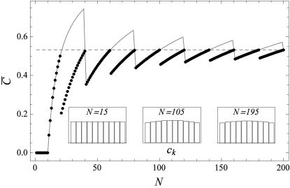
Figure 1: Average cost $\bar{C}$ as a function of level of phase discretization (number of phases $N$) for a $D=10$ dimensional system and the width of the step cost function $\sigma=\pi/10$. Gray line corresponds to the minimal cost obtainable with standard covariant measurements. Black dots correspond to the optimal strategy. In regimes where the optimal strategy outperforms the covariant one, the use of sub-covariant measurements is necessary. In this case improvement is due to the possibility of estimating phases that lie in the middle between the phases actually encoded in the state. Dashed line represent the value of the cost for the continuous limit $N\rightarrow\infty$. The inset depicts coefficients $c_{k}$ of the optimal input state at a given $N$.

We first assume we restrict ourselves to covariant measurements. We take $\Pi_{0}=D|e\rangle\langle e|$ while the optimal state we determine performing determining the vector corresponding to the minimal eigenvalue of matrix $A$ as defined in Eq.  (6). The results of the above procedure are depicted as a gray line in Fig. 1, for an exemplary case $D=10$ and $\sigma=\pi/10$. We can observe an apparently paradoxical behavior of the cost for some $N$ is above the one achieved in the continuous limit, which could be phrased in a way that discriminating a subset of states is more difficult than the whole set, a clear contradiction.

In order to remedy for this apparent paradox one should go beyond the standard covariant measurement class and consider the possibility of estimating phases which are not inside the set of encoded phases. In the considered case it is enough to include shifted-covariant measurements where the estimated phases correspond not to $\varphi_{n}=n\theta$ but to values exactly in between the actual phases encoded in the state., i.e. $\varphi_{n}+\theta/2$. In other words we should replace $\Pi_{0}$ with $\Pi_{\frac{1}{2}\theta}=DU_{\frac{1}{2}\theta}|e\rangle\langle e|U^{\dagger}_{\frac{1}{2}\theta}$. This is a special case of the class of measurements we refer to as sub-covariant measurements, which are described in a formal way in Sec. VI. Depending on the value of $N$ one should switch between the two strategies. The resulting minimal cost is depicted as black dots in Fig. 1.

The results are easy to understand. For $N\leq 10$, $\bar{C}=0$ as expected. Then for $11\leq N\leq 20$ the curve follows the $1-\frac{D}{N}$ formula corresponding to the optimal phase discrimination problem. At $N=21$, we observe a change due to the fact that the separation between the phases $2\pi/21$ is smaller than $\sigma$ and hence two phases can fit into the width of the cost function. The optimal measurement in this case corresponds to sub-covariant measurement. Another transition happens at $N=41$. This a point where $\sigma>2\theta$ and hence three phases can fit into one width of the cost function. At this point we recover the optimality of the standard covariant measurement. This situation repeats itself at every $N=k\times 20+1$, switching back and forth between the optimal covariant and shifted-covariant strategies.

In the continuous limit $N\rightarrow\infty$ we may of course use the standard covariant measurements. Plugging in $\Pi_{0}=D|e\rangle\langle e|$ into (3) and integrating over $\varphi$ for our step function cost we get:

$$\bar{C}=\langle\varphi_{0}|B|\varphi_{0}\rangle,\quad B_{jk}=\begin{cases}1-\frac{\sigma}{2\pi}&j=k\\ -\frac{1}{\pi(j-k)}\sin[\sigma(j-k)/2]&j\neq k.\end{cases}$$ (9)

The eigenproblem of matrix $B$ is well known from Fourier analysis Slepian (1978) and has also been studied in the context of quantum communication Hall and Fuss (1991); Hall (1993). The optimal input state is the eigenvector of matrix $B$ corresponding to the smallest eigenvalue which is then the minimal cost. The coefficients of this optimal eigenvector form a Discrete Prolate Spheroidal Sequence (DPSS) Slepian (1978). The smallest eigenvalue (minimal cost) corresponding to the DPSS eigenvector is plotted as a dashed line in Fig. 1. Note that thanks to the use of sub-covariant measurement the optimal cost for finite $N$ never exceeds the one corresponding to the continuous limit which should be the case as the continuous phase estimation should be never be less difficult than the discrete one.

V General cost function

Having studied this particular two examples, let us move on to a more general discussion where we will provide some general statements without specifying a particular form of the cost function. We consider a general cost function given by

$$C(\varphi)=\sum\limits_{m=0}^{M}\alpha_{m}\cos(m\varphi),$$ (10)

where the Fourier series structure of the parametrization reflects the periodicity of the function and we will refer to $M$ as order of the cost function. For the cost function to be meaningful, the coefficients $\alpha_{m}$ should be such to make $C(\varphi)\geq 0$, and $C(0)=0$. Let us first restrict to proper covariant measurements, so assume $\tilde{\varphi}\in\mathcal{S}_{N}$, and $\Pi_{\tilde{\varphi}}=U_{\tilde{\varphi}}\Pi_{0}U_{\tilde{\varphi}}^{\dagger}$. After inserting the cost function (10) and the explicit parametrization of the input state $|\varphi_{0}\rangle=\sum_{k}c_{k}|k\rangle$ to (5) the average cost reads:

$$\bar{C}=\sum\limits_{m=0}^{M}\alpha_{m}\frac{1}{N}\sum_{n=0}^{N-1}\cos(mn\theta)\sum_{j,k=0}^{D-1}\left(\Pi_{0}\right)_{jk}c_{j}c_{k}^{*}e^{i(j-k)n\theta}.$$ (11)

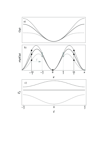
Figure 2: Difference in performance between covariant and shifted-covariant measurements in discrete phase estimation illustrated for a simple case of a qubit $D=2$ and three phases $N=3$. Generic behavior is depicted using three representative cost functions plotted in a): the standard cost function $C_{0}=4\sin^{2}\frac{\varphi}{2}$ (solid) as well as exemplary second order cost functions which approximate $\varphi^{2}$ for small $\varphi$ but are above or below the standard cost function respectively: $C_{1}=\frac{15}{6}-\frac{8}{3}\cos{\varphi}+\frac{1}{6}\cos{2\varphi}$ (dashed), $C_{2}=\frac{5}{4}-\cos\varphi-\frac{1}{4}\cos(2\varphi)$ (dotted). In b) difference between covariant measurement and shifted-covariant measurement, where the shift parameter is chosen to be $\xi=\pi/3$, is depicted as different sampling of the probability weighted cost function $\sigma(\varphi)C(\varphi)$. In general, for symmetric cost and probability distributions, the average cost $\bar{C}_{\xi}$ is going to have two extremal points at $\xi=0$ (covariant measurement) and $\xi=\pi/N=\pi/3$ (shifted-covariant measurement). Depending on the character of the average cost function the minimum is achieved at one point or the other. In the presented example, the shift is advantageous for $C_{1}$ cost function but not for $C_{2}$ and is irrelevant for $C_{0}$ since for this first order cost function $D=2$ and $N=3$ imply that the continuous phase estimation limit has already been reached.

As already discussed when analyzing the standard phase estimation cost function, in case $N\leq D$, the cost can always be made zero.

Let us now consider $N\geq D+1$. Due to $\cos(mn\theta)$ factor while performing the sum over $n$, the following sums will appear $\sum_{n=0}^{N-1}e^{i[(j-k)\pm m]n2\pi/N}$. This sums will be nonzero iff $(j-k)\pm m=0,\pm N,\pm 2N,\dots$ If we now increase number of phases such that $N=D+M$, then $|(j-k)\pm m|<N$ and hence only terms where $(j-k)\pm m=0$, i.e. first $M$ off diagonal terms of the state, will contribute. This also means than increasing $N$ further will not change the resulting cost, as the same terms will enter in the formula.

Hence we can draw a general conclusion – after being given an arbitrary cost function with order $M$, we predict the minimal cost to be zero for $N\leq D$, and then increase up to $N=D+M$, at which point it already reaches its continuous limit. This also implies that for $N\leq D$ and $N\geq N+M$ standard covariant measurement will suffice to reach the optimal performance. However, one cannot a priori assume that covariant measurements will be also optimal in the regime $D<N<D+M$.

Let us now further analyze the structure of formula (11). We can write it in the following form:

$$\bar{C}=\sum\limits_{n=0}^{N}\sigma(\varphi_{n})C(\varphi_{n}),$$ (12)

where $\sigma(\varphi)=\mathrm{Tr}\left(|\varphi\rangle\langle\varphi|\Pi_{0}\right)/N$. Intuitively, the continuous estimation corresponds to integrating the function $\sigma(\varphi)C(\varphi)$ from $0$ to $2\pi$, while discrete estimation corresponds to summing discretely probed values of this function. The simplest step beyond the covariant strategy is to introduce a non-zero offset $\xi$:

$$\bar{C}_{\xi}=\sum\limits_{n=0}^{N}\sigma(\varphi_{n}+\xi)C(\varphi_{n}+\xi),$$ (13)

i.e. to probe the function $\sigma(\varphi)C(\varphi)$ at different values of $\varphi$. This physically is equivalent to providing estimated phases outside the set of true phases, but still keeping an equal number of true and estimated phases. This is what we referred to before as shifted-covariant measurement.

Due to natural symmetry of the problem considered, both $C(\varphi)$ and $\sigma(\varphi)$ are symmetric functions and hence also probability weighted cost function $\sigma(\varphi)C(\varphi)$. This implies that $\bar{C}_{\xi}$ has an extremum at $\xi=0$. This also implies that another extremum should appear at $\xi=\pi/N$ corresponding to a shift by half the interval between the encoded phases—increasing or decreasing the value od $\xi$ around $\xi=\pi/N$ has the same effect on $\bar{C}_{\xi}$ as it can be seen as the same operation performed on original weighted cost function or on its reflection around $\varphi=0$ which is the same due to symmetry of the probability weighted cost function. We provide an illustrative example of this generic behavior in Fig. 2 for a simple qubit case $D=2$ and $N=3$ phases. In principle, there can be more extrema but we did not find them for any reasonable cost function studied. We did however observe additional extrema when considering mutual information as the figure of merit as outlined in Sec. VIII.

VI Sub-covariant measurements

In order to put our results in a more rigorous mathematical framework, we provide here a general theory of sub-covariant measurements, that help to remedy the apparent contradictions one may arrive at when applying the theory of standard covariant measurements to discrete parameter estimation problems, of which discrete phase estimation is a special case. We would like to stress that this concept is completely general and may used in an arbitrary discrete parameter estimation models beyond phase estimation. For this reason we will formulate it in a general way, where an estimation model arises as a result of choosing a subgroup $H$ of a group $G$ that generates the original continuous estimation problem. Note that we do not even insist that the group $H$ is discrete here, as this will not be relevant for the general discussion, hence the idea may applied even beyond the problem of discrete parameter estimation.

Let $G$ be a group and $H$ be a subgroup of $G$. We associate elements of $H$ with possible true values of a quantum parameter encoded in a state and elements of $G$ with possible measurement outcomes which are also the possible estimated values of the parameter. By $e$ we denote the neutral element of $G$. Let $U_{g}$ be a unitary representation of group $G$ on the Hilbert space of interest.

Definition. A POVM measurement $\{\Pi_{\tilde{g}}\}$ is sub-covariant with respect to subgroup $H\leq G$ if and only if

$$\forall_{h\in H,\tilde{g}\in G}U_{h}\Pi_{\tilde{g}}U_{h}^{\dagger}=\Pi_{h\tilde{g}}.$$ (14)

Let us observe that according to the above definition every measurement sub-covariant with respect to subgroup $H$ is uniquely defined by a family of operators $\{\Pi_{\gamma}\}_{\gamma\in G/H}$ by the following relation:

$$\Pi_{\tilde{g}}=U_{h}\Pi_{\gamma}U_{h}^{\dagger},$$ (15)

where $\tilde{g}=h\gamma$.

Theorem. If the estimation problem is sub-covariant with respect to $H\leq G$, i.e.: (i) $dh$—Haar measure on $H$, (ii) $\rho_{h}=U_{h}\rho_{e}U_{h}^{\dagger}$ for every $h\in H$ and (iii) $C(g^{\prime\prime}g^{\prime},g^{\prime\prime}g)=C(g^{\prime},g)$ for every $g,g^{\prime},g^{\prime\prime}\in G$, then we can choose the optimal measurement from measurements sub-covariant with respect to $H\leq G$.

Proof: Let $\{\Pi^{\mathrm{opt}}_{\tilde{g}}\}$ be the optimal measurement which minimizes the average cost

$$\bar{C}(\Pi^{\mathrm{opt}}_{\tilde{g}})=\int\limits_{H}dh\int\limits_{G}d\tilde{g}\operatorname{Tr}(\Pi^{\mathrm{opt}}_{\tilde{g}}\rho_{h})C(h,\tilde{g}).$$ (16)

We define

$$\Pi^{\mathrm{cov}}_{\tilde{g}}=\int\limits_{H}dh^{\prime}U_{h^{\prime}}^{\dagger}\Pi^{\mathrm{opt}}_{h^{\prime}\tilde{g}}U_{h^{\prime}}.$$ (17)

Then $\Pi^{\mathrm{cov}}_{\tilde{g}}$ is sub-covariant with respect to $H$ since:

$$U_{h}\Pi^{\mathrm{cov}}_{\tilde{g}}U_{h}^{\dagger}=U_{h}\int\limits_{H}dh^{\prime}U_{h^{\prime}}^{\dagger}\Pi^{\mathrm{opt}}_{\tilde{g}}U_{h^{\prime}}U_{h}^{\dagger}=\\ =\int\limits_{H}dh^{\prime}U_{hh^{\prime-1}}\Pi^{\mathrm{opt}}_{h^{\prime}\tilde{g}}U_{h^{\prime}h^{-1}}=\int\limits_{H}dh^{\prime}U_{h^{\prime}}^{\dagger}\Pi^{\mathrm{opt}}_{h^{\prime}h\tilde{g}}U_{h^{\prime}}=\Pi^{\mathrm{cov}}_{h\tilde{g}},$$ (18)

where in the last equality we have we substituted $h^{\prime}\rightarrow h^{\prime}h$, making use of the Haar measure property. Moreover, measurement $\Pi^{\mathrm{cov}}_{\tilde{g}}$ yields the same cost as $\Pi^{\mathrm{opt}}_{\tilde{g}}$, which can be seen as follows:

$$\bar{C}(\Pi^{\mathrm{cov}}_{\tilde{g}})=\int\limits_{H}dh\int\limits_{G}d\tilde{g}\operatorname{Tr}(\Pi^{\mathrm{cov}}_{\tilde{g}}\rho_{h})C(h,\tilde{g})=\\ =\int\limits_{H}dh\int\limits_{G}d\tilde{g}\operatorname{Tr}(\int\limits_{H}dh^{\prime}U_{h^{\prime}}^{\dagger}\Pi^{\mathrm{opt}}_{h^{\prime}\tilde{g}}U_{h^{\prime}}U_{h}\rho_{e}U_{h}^{\dagger})C(h,\tilde{g})=\\ =\int\limits_{H}dh\int\limits_{G}d\tilde{g}\int\limits_{H}dh^{\prime}\operatorname{Tr}(U_{hh^{\prime}}^{\dagger}\Pi^{\mathrm{opt}}_{h^{\prime}\tilde{g}}U_{hh^{\prime}}\rho_{e})C(h,\tilde{g})=\\ =\int\limits_{H}dh\int\limits_{G}d\tilde{g}\int\limits_{H}dh^{\prime}\operatorname{Tr}(U_{h}^{\dagger}\Pi^{\mathrm{opt}}_{\tilde{g}}U_{h}\rho_{e})C(h^{\prime-1}h,h^{\prime-1}\tilde{g})=\\ =\int\limits_{H}dh\int\limits_{G}d\tilde{g}\underbrace{\int\limits_{H}dh^{\prime}}_{=1}\operatorname{Tr}(\Pi^{\mathrm{opt}}_{\tilde{g}}\rho_{h})C(h,\tilde{g})=\bar{C}(\Pi^{\mathrm{opt}}_{\tilde{g}}),$$ (19)

where in the third line we have substituted $h\rightarrow h^{\prime-1}h,\tilde{g}\rightarrow h^{\prime-1}\tilde{g}$. This ends the proof $\square$.

Unlike in the full-covariant estimation problem, the search for the optimal measurement is not restricted here to identifying a single seed POVM $\Pi_{0}$, but rather a whole set $\Pi_{\gamma}$ where $\gamma\in G/H$. Still, this fact may significantly speed up the numerical search for the optimal estimation strategy as for sub-covariant measurements the average cost simplifies to:

$$\bar{C}=\int\limits_{G/H}d\gamma\int\limits_{H}dh\operatorname{Tr}(U_{h}\Pi_{\gamma}U_{h}^{\dagger}\rho)C(0,h\gamma).$$ (20)

Let us now discuss the relation of the above abstract and general theory with the phase estimation problem, especially with the examples presented in Secs. IV and V. In the continuous phase estimation problem $H=U(1)$ and sub-covariant measurements are not useful since there is no relevant group $G$ of which $H$ would be a nontrivial subgroup. In the discrete phase estimation problem $H=U_{N}$, and $\int_{H}dh\rightarrow\sum_{n=0}^{N-1}$, while in general $G=U(1)$. Hence the task is to find seed POVM set $\Pi_{\gamma}$, where $\gamma\in[0,\theta)=U(1)/U_{N}$. However, is is not always necessary to consider the full $G=U(1)$ group as it might be the case that the cost is minimal already for another discrete group $G=U_{lN}$, $l\in\mathbb{Z}$. An example is the shifted-covariant strategy optimal for some values of $N$ in Secs. IV and V, which corresponds to $H=U_{N}$, $G=U_{2N}$ and the seed POVM set {0, $DU_{\frac{\pi}{N}}|e\rangle\langle e|U^{\dagger}_{\frac{\pi}{N}}$}.

Let us also note that in the examples of discrete phase estimation discussed in the preceding sections we have not identified situations where more than one nonzero seed POVM would be necessary, and the optimal performance could always be reached by shifted-covariant measurements, which are the simplest non-trivial example of sub-covariant strategies. We expect, however, that for more involved discrete estimation problems more general class of measurements might be required. Therefore, in the next Sec. VII we provide a general algorithm to search for optimal sub-covariant strategies.

VII Algorithm for identifying the optimal discrete phase estimation strategy

Here we show how to effectively use the concept of sub-covariant measurements in order to numerically find the optimal discrete parameter estimation problems. For concreteness, we will focus on dicrete phase estimation, but the procedure can be directly generalized to any subgroup estimation problem using the framework described in Sec. VI.

First assume for the moment that the input state is fixed. We know that we can look for the optimal measurement/estimation strategy within the class of sub-covariant measurements. Hence we need to find the optimal seed POVM set $\Pi_{\gamma}$, where $\gamma\in[0,\theta)=U(1)/U_{N}$. Clearly looking for continuous family of operators is not feasible numerically. Still one can proceed in steps. Let us define sets containing an increasing number of seed measurement operators: $\mathcal{P}_{1}=\{\Pi_{0}\}$, $\mathcal{P}_{2}=\{\Pi_{0},\Pi_{\frac{1}{2}\theta}\}$, $\mathcal{P}_{3}=\{\Pi_{0},\Pi_{\frac{1}{3}\theta},\Pi_{\frac{2}{3}\theta}\}$ etc. Considering a given number $S$ of seed measurements, we minimize $\bar{C}$ over operators $\Pi_{s\theta/S}$, where $s\in\{0,\dots,S-1\}$, with the following constraints: $\Pi_{\frac{s}{S}\theta}\geq 0$, $\frac{1}{N}\sum_{s=0}^{S-1}\sum_{n=0}^{N-1}U_{n\theta}\Pi_{\frac{s}{S}\theta}U_{n\theta}^{\dagger}=\openone$. This is a standard semi-definite program and can be solved efficiently using e.g. the CVX package for Matlab Grant and Boyd (2012). We proceed by increasing $S$ and once we observe that further increase in $S$ does not reduce the cost we stop.

In order to find the optimal input state as well, one should adapt an iterative approach, as proposed in Demkowicz-Dobrzański (2011); Macieszczak et al. (2014), where the search for the optimal measurements is interleaved with the search for the optimal state. Applying the general form of Eq. (20) to our case of discrete quantum phase estimation, we obtain:

$$\bar{C}=\langle\varphi_{0}|A|\varphi_{0}\rangle,\quad A=\frac{1}{N}\sum_{s=0}^{S-1}\sum_{n=0}^{N-1}U_{n\theta}\Pi_{\frac{s}{S}\theta}U_{n\theta}^{\dagger}C(n\theta+\tfrac{s}{S}\theta).$$ (21)

We see that given a particular sub-covariant measurement, the search for the state minimizing the mean cost is equivalent to the search of an eigenvector corresponding to the minimal eigenvalue of the matrix $A$. By iterating the above scheme of finding the measurement optimal for a particular input state, and the the state optimal for a particular measurement one arrives at the fully optimal solution.

In particular, we have followed this procedure to confirm that the discrimination strategy described in Sec. II, based on switching between covariant and shifted-covariant measurements was indeed optimal.

VIII Mutual information as a figure of merit

In previous sections we have pursued an approach to quantum estimation/discrimination problems focused on minimization of Bayesian cost functions. This is a natural framework for determining optimal protocols in single-shot estimation/discrimination scenarios. One can, however, look at the discrete phase estimation setting as an example of a communication protocol, which is supposed to be repeated many times. In such situations a natural figure of merit is the mutual information between the encoded phases and measurement results which quantifies how many bits of noiseless information can be effectively transmitted per single use of the considered quantum channel.

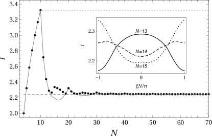
Figure 3: Mutual information vs. number of phases depicted for a $D=10$ dimensional system. Black dots represent the shifted-covariant measurements optimized over the shift parameter $\xi$ for each $N$, while solid gray line corresponds to the covariant measurements ($\xi=0$). For $N<D$, the shifted-covariant and covariant strategies are equivalent and saturate the Holevo bound (with Holevo quantity shown as dotted gray line). For $N\geq D$ the covariant and shifted-covariant strategies cease to yield the same results; the mutual information is greater or equal the continuous limit (dashed gray) for any $N$ only for the optimal shifted-covariant strategy. The inset shows the mutual information vs. the shift parameter $\xi$; the maxima at $\xi=0$, $0<\xi<\pi/N,$ and $\xi=\pi/N$ are observed for the exemplary cases of $N=13$ (solid), $N=14$ (dashed) and $N=15$ (dotted), respectively.

Given equiprobable phase encoded input states $|\varphi_{n}\rangle=U_{\varphi_{n}}|\varphi_{0}\rangle$, $\varphi_{n}=n\theta$, $n=0,\dots N-1$, and POVM measurement $\left\{\Pi_{m}\right\}$, the resulting joined probability distribution of symbol $n$ being sent and measurement outcome $m$ being registers reads:

$$p_{nm}=\frac{1}{N}\mathrm{Tr}(|\varphi_{n}\rangle\langle\varphi_{n}|\Pi_{m}),$$ (22)

while the corresponding mutual information reads:

$$I=\sum_{mn}H\left(p_{nm}\right)-\sum_{n}H\left(\sum_{m}p_{nm}\right)-\sum_{m}H\left(\sum_{n}P_{nm}\right),$$ (23)

where $H(x)=-x\log_{2}x$. The optimal protocol, from this point of view, is now the one that maximizes $I$ over the choice of input state $|\varphi_{0}\rangle$ and measurements $\{\Pi_{m}\}$.

Unlike the Bayesian cost, here $I$ is nonlinear both in measurement and the input state which makes the maximization of $I$ much more challenging. For covariant problems, there is no general theorem on the optimality of covariant measurements in this case, except for the situation when the states used are generated by the action of an irreducible representation of a group Davies (1978); Sasaki et al. (1999). In our case the $U(1)$ representation is clearly reducible and hence Davies theorem cannot be invoked. Still, one can bound the maximal achievable mutual information using the famous Holevo bound Holevo (1982). For our problem this bound implies:

$$I\leq\chi=S\left(\frac{1}{N}\sum_{n=0}^{N-1}|\varphi_{n}\rangle\langle\varphi_{n}|\right),$$ (24)

where $S(\rho)=-\mathrm{Tr}\rho\log_{2}\rho$ is the von Neumann entropy. For $N\leq D$, maximum $\chi$ corresponds to situation where we have $N$ orthogonal states $|\varphi_{n}\rangle$ and $\chi=\log_{2}N$. This bound can simply be achieved by using exactly the same strategy as described when minimizing Bayesian cost for $N\leq D$. Since $N$ orthogonal states are perfectly distinguishable by performing measurement in the basis containing the input states we can obtain $I=\log_{2}N$, saturating the Holevo bound and proving that this strategy is indeed optimal. In general the Holevo bound can never be larger than $\log_{2}D$ (maximum entropy is reached for $\rho=\openone/D$), hence for $N>D$ the bound has the form $I\leq\log_{2}D$ and does not further increase with $N$. Even though this bound cannot be in general achieved, it has been shown Maccone et al. (2017) that in the limit of continuous phase estimation $N\rightarrow\infty$, and large dimensions $D\rightarrow\infty$ one can reach almost optimal performance $I\approx\log_{2}D-1.2199$. This performance can be achieved using a strategy utilizing an equal superposition input states $|\varphi_{0}\rangle=|e\rangle=\frac{1}{\sqrt{D}}\sum_{k=0}^{D-1}|k\rangle$ and standard covariant continuous POVM, $\Pi_{\tilde{\varphi}}=\frac{D}{2\pi}U_{\tilde{\varphi}}|e\rangle\langle e|U_{\tilde{\varphi}}^{\dagger}$.

While studying discrete-to-continuous transition using mutual information figure of merit we will employ the above coding-decoding strategy. When going from the case $N=D$, where the mutual information can be made equal to the Holevo bound, to $N\rightarrow\infty$ (continuous regime) the accessible mutual information can only decrease, hence, we can sensibly expect that, since in the continuous limit the above described procedure performs almost optimally, it performs close to optimal also in the discrete case. Similarly as in the Bayesian approach, however, we have observed that it is essential to consider shifted-covariant measurements to obtain optimal performance. Note that when dealing with mutual information, there is no issue with the set of estimated values, as we deal solely with probability distribution. Still, when considering the specific class of POVMs as described above, we can naturally define a shifted-covariant POVM as $\Pi^{\xi}_{\tilde{\varphi}}=\frac{D}{2\pi}U_{\tilde{\varphi}+\xi}|e\rangle\langle e|U_{\tilde{\varphi}+\xi}^{\dagger}$. In Fig. 3 we depict the results for the discrete-to-continuous transition for $D=10$. Interestingly, in order to reach the optimal mutual information we occasionally have encountered situations where the optimum was reached for $0<\xi<\pi/N$, unlike in Bayesian examples studied where either $\xi=0$ and $\xi=\pi/N$ shifts were optimal. This is due to much more more involved structure of the mutual information potential leading to more than two local extrema while changing the shift parameter $\xi$.

We leave it as an open question, whether the above described strategy is optimal, and in particular whether more general measurements, that go beyond the class shifted-covariant measurements, could be useful in increasing the mutual information which is known to be the case in some communication problems Shor (2000).

IX Conclusions

In this paper, we have provided methods and results concerning the discrete phase estimation problem and its transition to the continuous limit. We have studied the transition for different cost functions and showed that in general one may need to go beyond the standard concept of covariant measurements and use a more general form—sub-covariant measurements introduced in this work.

We believe that these results may find their applicability in quantum communication theory where phase shift keying protocols involve encoding a discrete set of phases on the transmitted states. We also see this work as a first step towards better understanding a general problem of digital-to-analog transition in decoding and encoding information using quantum states, e.g. in quantum reading protocols Pirandola (2011).

References

- Hariharan (2003) P. Hariharan, Optical interferometry (Elsevier, Amsterdam, 2003).
- Cronin et al. (2009) A. D. Cronin, J. Schmiedmayer, and D. E. Pritchard, Rev. Mod. Phys. 81, 1051 (2009).
- Helstrom (1976) C. W. Helstrom, Quantum detection and estimation theory (Academic press, New York, 1976).
- Holevo (1982) A. S. Holevo, Probabilistic and Statistical Aspects of Quantum Theory (North Holland, Amsterdam, 1982).
- Giovannetti et al. (2011) V. Giovannetti, S. Lloyd, and L. Maccone, Nature Photonics 5, 222 (2011).
- Toth and Apellaniz (2014) G. Toth and I. Apellaniz, J. Phys. A: Math. Theor. 47, 424006 (2014).
- Demkowicz-Dobrzanski et al. (2015) R. Demkowicz-Dobrzanski, M. Jarzyna, and J. Kołodyński, in Progress in Optics, Vol. 60, edited by E. Wolf (Elsevier, 2015) pp. 345–435.
- Pezzè et al. (2016) L. Pezzè, A. Smerzi, M. K. Oberthaler, R. Schmied, and P. Treutlein, ArXiv e-prints (2016), arXiv:1609.01609 [quant-ph] .
- Caves (1981) C. M. Caves, Phys. Rev. D 23, 1693 (1981).
- Yurke et al. (1986) B. Yurke, S. L. McCall, and J. R. Klauder, Phys. Rev. A 33, 4033 (1986).
- Holland and Burnett (1993) M. J. Holland and K. Burnett, Phys. Rev. Lett. 71, 1355 (1993).
- Dowling (1998) J. P. Dowling, Phys, Rev. A 57, 4736 (1998).
- Berry and Wiseman (2000) D. W. Berry and H. M. Wiseman, Phys. Rev. Lett. 85, 5098 (2000).
- Huelga et al. (1997) S. F. Huelga, C. Macchiavello, T. Pellizzari, A. K. Ekert, M. B. Plenio, and J. I. Cirac, Phys. Rev. Lett. 79, 3865 (1997).
- Shaji and Caves (2007) A. Shaji and C. M. Caves, Phys. Rev. A 76, 032111 (2007).
- Dorner et al. (2009) U. Dorner, R. Demkowicz-Dobrzański, B. J. Smith, J. S. Lundeen, W. Wasilewski, K. Banaszek, and I. A. Walmsley, Phys. Rev. Lett. 102, 040403 (2009).
- Knysh et al. (2011) S. Knysh, V. N. Smelyanskiy, and G. A. Durkin, Phys. Rev. A 83, 021804 (2011).
- Genoni et al. (2011) M. G. Genoni, S. Olivares, and M. G. A. Paris, Phys. Rev. Lett. 106, 153603 (2011).
- Escher et al. (2011) B. M. Escher, R. L. de Matos Filho, and L. Davidovich, Nature Phys. 7, 406 (2011).
- Demkowicz-Dobrzański et al. (2012) R. Demkowicz-Dobrzański, M. Guţă, and J. Kołodyński, Nat. Commun. 3, 1063 (2012).
- Braunstein and Caves (1994) S. L. Braunstein and C. M. Caves, Phys. Rev. Lett. 72, 3439 (1994).
- Demkowicz-Dobrzański (2011) R. Demkowicz-Dobrzański, Phys. Rev. A 83, 061802 (2011).
- Hall and Wiseman (2012) M. J. W. Hall and H. M. Wiseman, New J. Phys. 14, 033040 (2012).
- Jarzyna and Demkowicz-Dobrzański (2015) M. Jarzyna and R. Demkowicz-Dobrzański, New Journal of Physics 17, 013010 (2015).
- Kitayama (2014) K. Kitayama, Optical Code Division Multiple Access. A practical Perspective (Cambridge University Press, Cambridge, 2014).
- Müller and Marquardt (2015) C. R. Müller and C. Marquardt, New Journal of Physics 17, 032003 (2015).
- Jarzyna et al. (2016) M. Jarzyna, V. Lipińska, A. Klimek, K. Banaszek, and M. G. A. Paris, Opt. Express 24, 1693 (2016).
- Brune et al. (2008) M. Brune, J. Bernu, C. Guerlin, S. Deléglise, C. Sayrin, S. Gleyzes, S. Kuhr, I. Dotsenko, J. M. Raimond, and S. Haroche, Phys. Rev. Lett. 101, 240402 (2008).
- Barnett and Croke (2009) S. M. Barnett and S. Croke, Adv. Opt. Photon. 1, 238 (2009).
- Ramsey (1980) N. F. Ramsey, Physics Today 33, 25 (1980).
- Nielsen and Chuang (2000) M. A. Nielsen and I. L. Chuang, Quantum Computing and Quantum Information (Cambridge University Press, Cambridge, 2000).
- Slepian (1978) D. Slepian, Bell System Technical Journal 57, 1371 (1978).
- Hall and Fuss (1991) M. J. W. Hall and I. G. Fuss, Quantum Optics: Journal of the European Optical Society Part B 3, 147 (1991).
- Hall (1993) M. J. W. Hall, Journal of Modern Optics 40, 809 (1993).
- Grant and Boyd (2012) M. Grant and S. Boyd, “Cvx: Matlab software for disciplined convex programming,” (2012).
- Macieszczak et al. (2014) K. Macieszczak, M. Fraas, and R. Demkowicz-Dobrzański, New Journal of Physics 16, 113002 (2014).
- Davies (1978) E. Davies, IEEE Transactions on Information Theory 24, 596 (1978).
- Sasaki et al. (1999) M. Sasaki, S. M. Barnett, R. Jozsa, M. Osaki, and O. Hirota, Phys. Rev. A 59, 3325 (1999).
- Maccone et al. (2017) L. Maccone, M. Hassani, and C. Macchiavello, ArXiv e-prints (2017), arXiv:1705.06666 [quant-ph] .
- Shor (2000) P. W. Shor, eprint arXiv:quant-ph/0009077 (2000), quant-ph/0009077 .
- Pirandola (2011) S. Pirandola, Phys. Rev. Lett. 106, 090504 (2011).