Feed-forward approximations to dynamic recurrent network architectures

Abstract

Recurrent neural network architectures can have useful computational properties, with complex temporal dynamics and input-sensitive attractor states. However, evaluation of recurrent dynamic architectures requires solution of systems of differential equations, and the number of evaluations required to determine their response to a given input can vary with the input, or can be indeterminate altogether in the case of oscillations or instability. In feed-forward networks, by contrast, only a single pass through the network is needed to determine the response to a given input. Modern machine-learning systems are designed to operate efficiently on feed-forward architectures. We hypothesised that two-layer feedforward architectures with simple, deterministic dynamics could approximate the responses of single-layer recurrent network architectures. By identifying the fixed-point responses of a given recurrent network, we trained two-layer networks to directly approximate the fixed-point response to a given input. These feed-forward networks then embodied useful computations, including competitive interactions, information transformations and noise rejection. Our approach was able to find useful approximations to recurrent networks, which can then be evaluated in linear and deterministic time complexity.

Introduction

With very few exceptions, biological networks of neurons are highly recurrent. For an extreme example, neurons in the primary visual cortical areas in mammalian brain make a majority of their synaptic connections between other neurons in the local vicinity (Binzegger et al.,, 2004). Recurrent networks can give rise to complex temporal dynamics and potentially beneficial emergent computational properties. For example, desired relationships between the activity of several neurons can be embedded in recurrent excitatory weights (Douglas et al.,, 1994; Hahnloser,, 2003; Rutishauser and Douglas,, 2009); the dynamics of the network can then selectively amplify the desired representations while rejecting noise or undesired interpretations of an input (Ben-Yishai et al.,, 1995; Somers et al.,, 1995; Douglas and Martin,, 2007). Chaotic temporal dynamics present in reservoirs of randomly connected neurons can be exploited to selectively detect or generate robust temporal sequences (Maass et al.,, 2002; Sussillo and Abbott,, 2009; Laje and Buonomano,, 2013).

However, simulating dynamic recurrent networks to make use of their properties in artificial systems is inconvenient for several reasons. Such simulations are non-deterministic in terms of the time required to find an “answer” for a given input. This is because the dynamics of recurrent networks, especially stochastically-generated networks, may not be guaranteed to be stable for every input, and may indeed not be known in advance of a simulation. Even if stable fixed-point responses exist for every finite input, the time taken to reach these fixed points may differ depending on the input. This issue is exacerbated by the poor fit between simulations of recurrent networks and commodity computational architectures (i.e. CPU / GPU).

In contrast, recent successes in using feed-forward or unrolled “recurrent” architectures (Graves et al.,, 2013; Radford et al.,, 2015) have occurred hand in hand with development of computational systems optimised for evaluation of feed-forward networks (Collobert et al.,, 2011; Jia et al.,, 2014; Theano Development Team,, 2016). Modern approaches for distributed evaluation of large networks (Abadi et al.,, 2016) make feed-forward architectures very attractive for a range of applied computational tasks.

Here we examine whether the known beneficial computational properties of highly recurrent network architectures can be realised in feed-forward architectures. We take the approach of probing recurrent networks to quantify a mapping between inputs and fixed-point responses. We then train feed-forward networks to approximate this mapping, and compare the information-processing abilities of the recurrent networks with their feed-forward approximations.

Results

Recurrent networks and feed-forward approximations

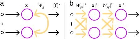
Figure 1: Recurrent and feed-forward network architectures. (a) Two-neuron recurrent architecture. Rectified-linear (ReLU) neurons ($\mathbf{x}$; circles) receive input ($\mathbf{i}$), and possibly reach a stable fixed point in activity ($\mathbf{f}$; the values of network activity $\mathbf{x}$ at the fixed point, if it exists) through recurrent interactions via weights $W_{R}$. (b) A $2\times 2$ neuron feed-forward architecture. Input $\mathbf{i}$ is transformed through two layers of ReLU neurons ($\mathbf{x}|^{1},\mathbf{x}|^{2}$) via all-to-all weight matrices $W_{FF}|^{1}$ and $W_{FF}|^{2}$. The activity $\mathbf{x}|^{2}$ of layer 2 is the output of the network. See Methods for more detail.

Fig. 1a shows an example of a simple 2-neuron single-layer recurrent network. The dynamics of each rectified-linear (or linear-threshold; or ReLU) neuron ($x_{j}$, composed into a vector of activity $\mathbf{x}$) is governed by a nonlinear differential equation

$$\tau\cdot\dot{x}+x=W_{R}\cdot\left[\mathbf{x}\right]^{+}\!+i$$ (1)

(see Methods), and evolves in response to the input i provided to the neuron, as well as the activity of the rest of the network $\mathbf{x}$ transformed by the recurrent synaptic weight matrix $W_{R}$. Here $\left[x\right]^{+}$denotes the linear-threshold transfer function $\left[x\right]^{+}=\max\left(x,0\right)$. Neglecting the potentially complex temporal dynamics of network activity, for this work we define the “result” of such a network as the rectified fixed-point response of the population activity of the network $\left[\mathbf{f}\thinspace\right]^{+}$, if a stable fixed point exists.

In the following, we approximate the mapping between network inputs $\mathbf{i}$ and network fixed points $\left[\mathbf{f}\right]^{+}$ using a family of feed-forward network architectures (Fig. 1b). For a recurrent network with $N=2$ neurons, the corresponding feed-forward approximation consisted of two layers, each consisting of $N=2$ ReLU neurons. All-to-all weight matrices $W_{FF}|^{1}$ and $W_{FF}|^{2}$ defined the connectivity between the network input ($\mathbf{i}$), the neurons of layer 1 ($\mathbf{x}|^{1}$), and the neurons of layer 2 ($\mathbf{x}|^{2}$). We use the notation $v|^{n}$ to refer to a variable $v$ within layer $n$. In some implementations of unrolled recurrent network architectures, weight matrices across several layers, representing multiple points in time, are tied together and trained as a group. We did not take that approach with our feed-forward networks, and permitted the weights for each layer to vary independently. The activity of $\mathbf{x}|^{2}$ were taken as the output of the network. In contrast to the recurrent network, neuron activations in the feed-forward approximation were given by deterministic feed-forward evaluation, with no temporal dynamics (Eq. 5; see Methods).

Small network architectures

Figure 2: Feed-forward approximation to the fixed-point mapping of a 2 neuron recurrent network, with real positive eigenvalues. (a) Recurrent dynamics for the system $W_{R}=\left[\begin{array}[]{cc}.4&.2\\ .8&.5\end{array}\right]$. Loci of recurrent network responses traced to fixed points (dots), from a matrix of inputs $\mathcal{I}$ arranged uniformly over the unit square $\left(-1,1\right)^{2}$ (solid square). Each line traces the locus of $\mathbf{x}$ in response to a single input $\mathbf{i}{}_{m}$ to the corresponding fixed point $\mathbf{f}_{m}$. The origin is indicated by the black cross. (b) Rectified fixed-point responses $\mathcal{F}\ni\left[\mathbf{f}_{m}\right]^{+}$ of the recurrent network (circles), overlaid with the corresponding feed-forward network response (dots). Orange lines connect poorly-mapped feed-forward responses to the corresponding recurrent fixed point. $\left\{W_{FF}^{1},W_{FF}^{2},\mathbf{b}_{FF}^{1},\mathbf{b}_{FF}^{2}\right\}=\left\{\left[\begin{array}[]{cc}4.06&2.20\\ 2.71&2.46\end{array}\right],\left[\begin{array}[]{cc}2.33&-0.51\\ 0.60&1.20\end{array}\right],\left[\begin{array}[]{c}.46\\ .21\end{array}\right],\left[\begin{array}[]{c}-2.34\\ -1.77\end{array}\right]\right\}$.

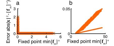
Figure 3: Errors in the feed-forward approximation occur mainly around the activation threshold. (a) Large differences between the output of the feed-forward approximation ($\mathbf{x}|^{2}$) and the rectified fixed-point of the recurrent network ($\left[\mathbf{f}_{m}\right]^{+}$) occur mostly when the activation of one recurrent unit is below threshold (i.e. $x_{1},x_{2}<0$; $\left[\textbf{f}_{m}\right]^{+}=0$). (b) Errors in generalization increase as the input to the network moves further outside the trained region ($\iota_{1},\iota_{2}>1$), but remain small.

We first investigated whether the dynamics of 2-neuron recurrent networks can be approximated by training a two-layer linear-threshold neuron (ReLU) network to directly map network inputs to fixed-point responses of the recurrent network. We obtained accurate feed-forward approximations for randomly chosen neuron recurrent networks that exhibited stable non-trival fixed points. Here we show two examples of networks with both non-oscillatory and oscillatory dynamics. Fig. 2 shows the result of approximating a 2-neuron recurrent network with positive real eigenvalues, which lead to stable fixed points with an expansive mapping of the input space.

We performed a random sampling of the input space by drawing uniform random variates from the unit square $\left(-1,1\right)^{2}$. For each input, we analysed the eigenspectrum and solved the dynamics of the recurrent network to determine whether a stable fixed-point response existed for that input, discarding inputs for which no stable fixed point existed. We therefore found a mapping between a set of inputs $\mathcal{I}$ and the set of corresponding fixed-point responses $\mathcal{F}$, which was used as training data to find an optimal feed-forward approximation to that mapping (see Methods). Fig. 2a shows the activity dynamics of the recurrent network, from a number of inputs to their corresponding fixed points.

Figure 4: Feed-forward approximation to a 2 neuron recurrent network with damped oscillatory dynamics and complex eigenvalues. (a) Recurrent dynamics for the system $W_{R}=\left[\begin{array}[]{cc}.70&.11\\ -.54&.98\end{array}\right]$. This network has complex eigenvalues, with damped oscillatory dynamics. (b) Recurrent fixed-point responses (circles) compared with feed-forward network responses (dots). $\left\{W_{FF}|^{1},W_{FF}|^{2},\mathbf{b}_{FF}|^{1},\mathbf{b}_{FF}|^{2}\right\}=\left\{\left[\begin{array}[]{cc}1.77&1.29\\ -0.54&6.89\end{array}\right],\left[\begin{array}[]{cc}0.23&-0.21\\ -4.35&1.49\end{array}\right],\left[\begin{array}[]{c}5.03\\ 0.84\end{array}\right],\left[\begin{array}[]{c}-10.03\\ -3.19\end{array}\right]\right\}$. Notations as in Fig. 2.

We used a stochastic gradient-descent optimisation algorithm with momentum and adaptive learning rates (Adam; Kingma and Ba,, 2015) to find a feed-forward network that approximated the mapping $\mathcal{I}\rightarrow\mathcal{F}$ by minimising the mean-square loss function $c=\nicefrac{{1}}{{2M}}\Sigma_{m=1}^{M}\left(\textbf{x}_{m}|^{2}-\left[\textbf{f}_{m}\right]^{+}\right)^{2}$ (see Methods). The Adam optimisation algorithm resulted in feed-forward approximations with smaller errors than training using direct gradient descent without momentum. Only fixed points in which all elements $\mathbf{f}_{m}>0$ were used for training. We found this approach to result in better approximations to recurrent fixed points. Since many inputs map to zero fixed point responses in the recurrent network (see Fig. 2a), the training process tended to over-emphasise them, leading to a poor representation of non-zero fixed points. Training was performed over randomly generated batches containing $M=50$ input to fixed-point mappings, and was halted when the batch training error smoothed over 100 batches converged.

Fig. 2b shows the $\mathcal{I}\rightarrow\mathcal{F}$ mapping produced by the best feed-forward network found after 16 500 training iterations. Inputs that lead to a non-zero response from both neurons were mapped with high accuracy (overlapping dots and circles).

Errors in the feed-forward approximation occurred mainly around the activation threshold (Fig. 3a). The feed-forward approximation also generalized well for inputs outside the training regime (i.e. $\iota_{1},\iota_{2}>1$; Fig. 3b). Generalization errors increased slowly further from the trained input space, but remained small. In this example, we were therefore able to train an accurate feed-forward approximation to the fixed-point dynamics of this simple recurrent network.

How does this approach fare, when applied to a recurrent network with more complex dynamics? Fig. 4 shows the result of approximating a 2-neuron recurrent network with a complex eigenvalue pair with positive real part, which leads to stable spiral fixed points. This recurrent network exhibited damped oscillatory dynamics when driven by constant inputs (Fig. 4a). Nevertheless, our approach of approximating the mapping $\mathcal{I}\rightarrow\mathcal{F}$ was successful. Fig. 4b shows a comparison between the recurrent and feed-forward network mappings. As before, errors in the feed-forward approximation were restricted to the area around the neuron activation threshold. Our approach is therefore able to find feed-forward approximations to recurrent networks with complex temporal dynamics.

Competitive networks with partitioned excitatory structure

Figure 5: Competition in a two-partition network. (a) A recurrent dynamic network with two all-or-nothing excitatory partitions (A and B), and a single global inhibitory neuron (Inh). The architecture of the feed-forward approximation network is as shown in Fig. 1. (b) Stimulating the partitions with a linear mixture of input currents $\left(0,1\right)$ (grey shading) provokes strong competition in the response of the partitions (note rapid switching between partition A and B when inputs are roughly equal). The feed-forward approximation (dashed lines) exhibits similar competitive switching to the recurrent network (solid lines). Recurrent network parameters: $\left\{N,w_{E},w_{I},\mathbf{b}\right\}=\left\{5,2.5,8,\mathbf{0}\right\}$.

There is growing evidence for network architectures in cortex that group excitatory neurons into soft-partitioned subnetworks (Yoshimura et al.,, 2005; Ko et al.,, 2011). Connections within these subnetworks are stronger and more prevalent (Cossell et al.,, 2015). Subnetwork membership may be defined by response similarity; neurons with correlated responses over long periods will therefore tend to be connected (Ko et al.,, 2011; Cossell et al.,, 2015; Lee et al.,, 2016). These rules for connection probability and strength can give rise to network architectures with complex dynamical and stability properties, including selective amplification and competition between partitions (Muir and Mrsic-Flogel,, 2015).

We investigated a simplified version of subnetwork partitioning, with all-or-nothing recurrent excitatory connectivity (Fig. 5a; see example matrix in Methods). Networks with this connectivity pattern exhibit strong recurrent recruitment of excitatory neurons within a given partition, coupled with strong competition between partitions mediated by shared inhibitory feedback. As a consequence the recurrent network can be viewed as solving a simple classification problem, whereby the network signals which is the greater of the summed input to partition A ($\iota_{1+2}=\iota_{1}+\iota_{2}$) or to partition B ($\iota_{3+4}=\iota_{3}+\iota_{4}$). In addition, the network signals an analogue value linearly related to the difference between the inputs. If $\iota_{1+2}>\iota_{3+4}$ then the network should respond by strong activation of $x_{1,2}$ and complete inactivation of $x_{3,4}$ (and vice versa for $\iota_{1+2}<\iota_{3+4}$ ).

We first examined the strength of competition present between excitatory partitions, by providing mixed input to both partitions, comparing the recurrent network response with the feed-forward approximation (Fig. 5b). Input was provided equally to both excitatory neurons in a partition, such that $\iota_{1}=\iota_{2}$ and $\iota_{3}=\iota_{4}$. For a given network evaluation, a single mixture was chosen such that $\sum\mathbf{i}$ was constant. When input to partition A was weak, input to partition B was strong, and vice versa. The recurrent network was permitted to reach a stable fixed point for a given static input mixture, and the feed-forward approximation was evaluated with the same input pattern.

The recurrent network exhibited strong competition between responses of the two excitatory partitions: only a single partition was active for a given network input, even when the input currents to the two partitions were almost equal. The feed-forward approximation exhibited very similar competition between responses of the two partitions as the recurrent network, also exhibiting sharp switching between the partition responses (Fig. 5b). In addition, the feed-forward network learned a good approximation to the analogue response of the recurrent network, as for the simpler networks of Figs 2–4.

Figure 6: Decision boundary is almost aligned between recurrent network and feed-forward approximation. Shown is the projection of the input space $\mathbf{i}$ into two dimensions $\iota_{1+2}=\iota_{1}+\iota_{2}$ and $\iota_{3+4}=\iota_{3}+\iota_{4}$. The ideal decision boundary of $\iota_{1+2}=\iota_{3+4}$ is indicated as a dashed horizontal line. The majority of inputs sampled close to the decision boundary resulted in the activation of the correct partition in both the recurrent network and feed-forward approximation (grey dots). The decision boundary of the feed-forward approximation was not perfectly aligned with that of the recurrent network, resulting in misclassification of some inputs close to the decision boundary (orange dots). Network parameters as in Fig. 5.

Although the feed-forward approximation was not trained explicitly as a classifier, we examined the extent to which the feed-forward approximation had learned the decision boundary implemented by the recurrent network (Fig. 6). Multi-layer feed-forward neural networks of course have a long history of being used as classifiers (e.g. Rumelhart et al.,, 1986; LeCun et al.,, 1989). The purpose of the approach presented here is to examine how well the feed-forward approximation has learned to mimic the boundaries between basins of attraction embedded in the recurrent dynamic network. This question is particularly interesting for larger and more complex recurrent networks, for which the boundaries between basins of attraction are not known a priori.

We examined the response of the feed-forward approximation close to the ideal decision boundary ($\iota_{1+2}=\iota_{3+4}$; dashed line in Fig. 6). We found that the majority of inputs were correctly classified by the feed-forward approximation, but the decision boundary of the feed-forward approximation was not perfectly aligned with the ideal, with the result that a minority of inputs close to the boundary were misclassified by the feed-forward approximation.

Line attractor networks

Figure 7: Feed-forward approximation recovers the weight structure of a recurrent ring model for orientation preference. (a) A schematic of a ring model for orientation preference. Excitatory neurons (outer ring) are arranged in order of preferred orientation ($\theta$). Recurrent excitatory connections upper arrows are modulated by similarity in $\theta$ (see Methods). Inhibitory connections (from central neuron; Inh) are made with all excitatory neurons. The architecture of the corresponding feed-forward approximation network is as shown in Fig. 1. Recurrent excitatory connections are shown for a single neuron, but are made identically from all excitatory neurons. (b) Recurrent weights $W_{R}$ implementing the ring model in a dynamic recurrent network. Inhibitory weights were weakened by a factor of 10 for visualisation. (c) Weights learned in a feed-forward approximation to the dynamics of a recurrent ring model. Note the neighbourhood pattern learned by the feed-forward network, similar to that of the recurrent network. Recurent weights $W_{R}$ and second-layer weights $W_{FF}|^{2}$ were scaled for visualisation purposes. Recurrent network parameters: $\left\{N,w_{e},w_{i},\mathbf{b}\right\}=\left\{40,2,5,\mathbf{0}\right\}$.

Neurons in primary visual cortex of primates and carnivores have individual preferences for the orientation of a line segment in visual space (Hubel and Wiesel,, 1962, 1968); neurons that prefer similar orientations are grouped together, and this preference changes smoothly across the surface of cortex (Bonhoeffer and Grinvald,, 1991; Blasdel,, 1992). Experimental work suggests that the sharp tuning of visual neurons for their preferred orientation arises through recurrent processing within the cortical network (Tsumoto et al.,, 1979), rather than being defined by structured inputs to each neuron from outside the local network (Hubel and Wiesel,, 1962). The recurrent processing hypothesis is also consistent with the fact that the majority of input synapses to each neuron arise from other nearby neurons, and not from visual input pathways (Peters and Payne,, 1993; Ahmed et al.,, 1994; Binzegger et al.,, 2004).

Several recurrent network models of mammalian cortex make use of the fact that the function of neurons changes smoothly across the surface of many cortical areas (Douglas et al.,, 1994; Ben-Yishai et al.,, 1995; Somers et al.,, 1995). The tight relationship between physical and functional space (i.e. the preferred orientation $\theta$ of a neuron) suggests that local neuronal connections should be made predominately between neurons with similar $\theta$, falling off with distance. In these recurrent models excitatory neurons are consequently arranged in a ring (therefore “ring models”; Fig. 7a), with smoothly-varying $\theta$ and with excitatory connection strength falling off with decreasing similarity in $\theta$. Inhibitory neurons are broadly tuned or untuned for preferred orientation in these models, and therefore make and receive connections with all excitatory neurons.

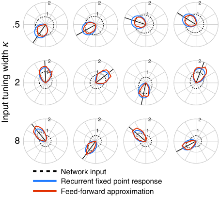
Figure 8: Sharpening of broadly-tuned input. Shown are polar plots of preferred orientation $\theta$ versus network response amplitude, for a given input (black dashed), for both the recurrent model (blue) and the feed-forward approximation (orange). Rows correspond to four examples each of input under increasing tuning sharpness $\kappa$ (indicated at left), and randomly-chosen $\Theta$ (black line in each example). Noise std. dev. $\zeta=0$ for these examples; common-mode input $\gamma=0.5$. All plots have identical scaling. Note the similarity between recurrent fixed point responses and the feed-forward approximation, and the consistency in response tuning over a range of broadly-tuned inputs patterns. Network parameters as in Fig. 7.

These ring models perform powerful and useful information processing tasks, which are supported by mechanisms of selective amplification through recurrent excitation, coupled with competitive interactions mediated by global inhibitory feedback (also known as winner-take all interactions; Douglas and Martin,, 2007). Single neurons exhibit consistent, sharp tuning for their preferred orientation $\theta$, in spite of poorly-tuned input. Ring networks are also able to reject significant noise in the input, to provide a clean interpretation of a noisy signal. Recurrent dynamics within the network establish a line attractor, whereby a set of stable response patterns that are translated versions of a common activity pattern are permitted by the network.

We investigated whether a feed-forward approximation to a simple ring model for orientation preference could capture useful information-processing features of the recurrent network. We trained a two-layer $40+40$ neuron network to approximate the fixed-point recurrent dynamics of a 40-neuron recurrent ring model network (see Methods). We generated the training mapping $\mathcal{I}\rightarrow\mathcal{F}$ by generating uniform random inputs $\mathbf{i}_{m}\sim\mathcal{U}\left(.5,1\right)$ and solving the dynamics of the recurrent network to identify the corresponding fixed points $\mathbf{f}_{m}$ (see Methods). We discarded inputs for which no corresponding fixed point could be found.

Fig. 7b shows the weight matrices for the two-layer network best approximating the recurrent dynamics, after 64 000 training iterations. Note that the neighbourhood relationships between similarly-tuned neurons is reflected in the learned feed-forward weight structure, which has been acquired solely by mimicking the fixed-point dynamics of the recurrent network (c.f. Fig. 7c). The locality of mapping between adjacent neuron indices was encouraged by initialising the feed-forward weights $W_{FF}|^{1}$ and $W_{FF}|^{2}$ to the identity matrix $I$ at the beginning of training (see Methods).

The ring model was designed to demonstrate how recurrent processing can lead to sharpening of broadly-tuned inputs. To investigate whether our feed-forward approximation exhibits similar functionality, we stimulated recurrent and feed-forward networks with broadly-tuned inputs (Fig. 8). Indeed, the responses of the feed-forward approximation were sharpened versions of the input, and had similar tuning sharpness as the recurrent network. Interestingly, the sharpness of response tuning of the feed-forward network did not change appreciably across a wide range of input tuning sharpnesses. The feed-forward approximation was therefore able to capture the main information-processing feature of the recurrent ring model.

Figure 9: Feed-forward approximations can mimic the noise rejection properties of the recurrent ring model. Rows correspond to four examples each of input under increasing noise std. dev. $\zeta$ (indicated at left), and randomly-chosen $\Theta$. Tuning sharpness $\kappa=4$; common-mode input $\gamma=0.5$. Network parameters and notations as in Figs 7 and 8.

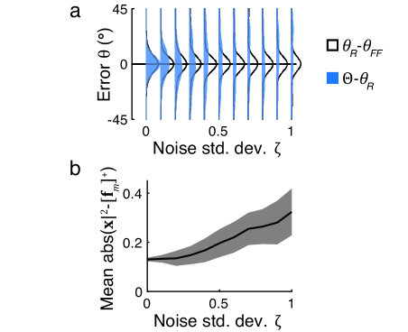
Figure 10: Noise rejection by the feed-forward approximation is robust over a range of noise amplitudes. (a) The error between the recurrent model angle of peak response $\theta_{R}$ and the feed-forward approximation angle of peak response $\theta_{FF}$ (black) was consistently small over all noise amplitudes $\zeta$. For increasing noise amplitudes, the ability of the recurrent model to correctly identify the orientation of the input $\theta_{\iota}$ degraded (blue). (b) The accuracy of the feed-forward approximation with respect to the recurrent model degraded gradually with increasing noise amplitude $\zeta$. Tuning sharpness $\kappa=4$; common-mode input $\gamma=0.5$. Network parameters as in Fig 7.

Noise rejection in the recurrent ring model is mediated by recurrent shaped excitatory amplification of responses, coupled with global inhibitory feedback. We investigated whether the feed-forward approximation was able to perform equivalent noise rejection, in the absence of recurrent excitatory amplification. We stimulated the network with tuned inputs, with increasing amounts of Normally-distributed noise with std. dev. $\zeta$ (Figs 9 and 10; see Methods).

We quantified the error in network responses in several ways. Firstly, the purpose of noise rejection in the recurrent model is to identify the orientation $\Theta$ of the underlying stimulus. We defined the angle of peak response $\theta_{R}$ as the preferred orientation $\theta$ of the neuron with peak response, i.e. $\theta_{j}:j=\arg\max x_{j}$, and defined $\theta_{FF}$ analogously for the feed-forward approximation. We then quantified the error in stimulus interpretation between the recurrent and feed-forward networks $\theta_{R}-\theta_{FF}$ (Fig. 10a, black). This error was consistently clustered around zero, highlighting the closeness of the feed-forward approximation to the behaviour of the recurrent model (see also examples in Fig. 9). As expected, the ability of both models to correctly identify the underlying stimulus orientation $\Theta$ degraded with increasing noise amplitude $\zeta$ (increasing errors $\Theta-\theta_{R}$, Fig. 10a, blue). The mean error between the response of the recurrent network and the feed-forward approximation $\textrm{mean}\left(\textrm{abs}\left\{\textbf{x}|^{2}-\left[\textbf{f}_{m}\right]^{+}\right\}\right)$ also increased with increasing noise amplitude $\zeta$ (Figs 9 and 10b).

The recurrent ring models perform common-mode input rejection, whereby the response of the recurrent dynamic network is unchanged by adding a common-mode offset to an input. This occurs through dynamic thresholding of the network response, provided by global inhibitory feedback. Our feed-forward approximations were trained with a fixed common-mode input $\gamma$ (see Methods). We examined the ability of the feed-forward approximations to generalise their responses given arbitrarily-scaled common mode input (Fig. 12). For feed-forward approximations trained with $\gamma=0.5$, we found that absolute approximation errors remained low for $\gamma\leq 2.0$ (i.e. error amplitudes $<1.0$). For larger $\gamma$, errors scaled linearly with the response of the feed-forward network, indicating that the approximation breaks down. This result suggests that matching of the input space to the training space is required for accurate approximation, either through appropriate selection of training inputs $\mathcal{I}$ or through input normalisation.

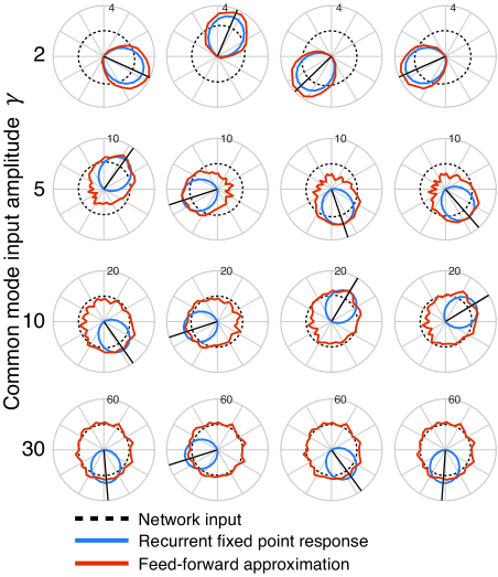
Figure 11: Common-mode input rejection fails for large common-mode amplitudes. Shown are examples of the recurrent network (blue) and the feed-forward approximation responses (orange) when driven with inputs with varying common-mode input amplitudes $\gamma$ (black dashed). The feed-forward approximation was trained with $\gamma=0.5$. While the recurrent dynamic network rejected common mode inputs over all amplitudes, the feed-forward approximation ceased to perform well for $\gamma>2$. For large $\gamma$, common-mode noise was not rejected by the feed-forward approximation (see Fig. 12).

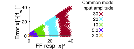
Figure 12: The feed-forward approximation cannot reject common-mode input of arbitrary amplitude. Shown is the error between the feed-forward approximation response $\mathbf{x}|^{2}$ and the recurrent dynamic network response $\left[\mathbf{f}_{m}\right]^{+}$ to a given input, as a function of the scale of the feed-forward response $\mathbf{x}|^{2}$, for a range of common mode input amplitudes $\gamma$. The feed-forward approximation was trained with $\gamma=0.5$. Errors for $\gamma<2$ were clustered close to zero. Network parameters as in Fig. 7.

Discussion

We investigated whether feed-forward neural networks could approximate the fixed-point responses of dynamic recurrent networks. We trained two-layer feed-forward architectures to replicate the input-to-fixed-point mapping of a dynamic recurrent networks. We found that for small arbitrary networks, larger networks with partitioned excitatory and inhibitory neurons, and multiple partitioned excitatory populations, as well as even larger networks embedding line attractors, two-layer feed-forward approximations were able to successfully reproduce the fixed-point responses of dynamic recurrent networks.

Feed-forward approximations reproduced the fixed-point responses for two-neuron dynamic recurrent networks, for recurrent networks with both simple and complex temporal dynamics (Figs 2 and 4). In the case of a dynamic recurrent network exhibiting competitive interactions between excitatory partitions, the feed-forward approximation accurately replicated competition between partitions (Fig. 5). Our approach was able to find a good approximation to a line attractor network with highly nonlinear dynamics — a soft winner-take-all “ring” model for preferred orientation. This was impressive considering that the training inputs provided to the network were uniformly randomly distributed, and did not take into account the line attractor computation performed by the recurrent network. The feed-forward approximation reproduced nonlinear input transformations and noise rejection, both of which are considered to be particularly useful features of recurrent computation in the model (Figs 8–12).

We found that the accuracy of the approximations degraded close to the activation thresholds of the feed-forward network (Fig. 3a). This may be due to the hard loss of gradient information below the activation threshold, in which case using units with a soft nonlinearity might alleviate this issue. However, the feed-forward approximations to the two-neuron recurrent networks generalized well for inputs outside the trained input space (Fig. 3b), with errors increasing slowly but remaining low for inputs well outside the training regime.

The feed-forward approximation to the recurrent ring model generalized well for inputs up to a factor of 4 outside the training regime (Fig. 12). However, the approximation broke down for inputs with larger amplitudes, in spite of the linear transfer functions present in each neuron. Nevertheless, this restriction simply entails the use of normalised input spaces to ensure accuracy of the approximation.

Our feed-forward approximations implicitly assume that only the fixed-point response to an input is important, and the temporal evolution of activity to reach that fixed point is ignored. Some modes of operation of dynamical recurrent networks explicitly make use of chaotic dynamics to detect and generate temporal activity sequences (Maass et al.,, 2002; Sussillo and Abbott,, 2009; Laje and Buonomano,, 2013). Computations that require access to activity trajectories will of course not be possible under the framework we proposed here. An approach might be possible where a network was trained with step-wise approximations to the dynamics of a recurrent network, but the purpose of our approximations was to obviate the use of iterative solutions. Since our feed-forward networks have no temporal dynamics, they also cannot capture complex dynamical behaviours such as damped oscillatory or limit cycle dynamics (Landsman et al.,, 2012).

The response of the feed-forward approximations to a given input does not depend on previous network activity, in the formulation presented here. Responses to temporal input sequences will therefore only be accurate if the time constant of input changes is much slower than the time constant of the dynamics of the original recurrent network, and if complex basins of attraction are not present. Related to this point, unrolled recurrent architectures such as LSTM networks have been employed to process discrete temporal input sequences (Hochreiter and Schmidhuber,, 1997; Liwicki et al.,, 2007). Our feed-forward approximations could be operated in a similar mode by augmenting the current input $\textbf{i}\left(t\right)$ with the previous fixed-point activity $\textbf{x}|^{2}\left(t-1\right)$.

Feed-forward approximations to dynamic recurrent systems are a powerful tool for capturing the information processing benefits of highly recurrent networks in conceptually and computationally simpler architectures. Information processing tasks such as selective amplification and noise rejection performed by recurrent dynamical networks can therefore be incorporated into feed-forward network architectures. Evaluation of the feed-forward approximations is deterministic in time, in contrast to seeking a fixed-point response in the dynamic recurrent network, where the time taken to reach a fixed-point response — and indeed the existence of a stable fixed point — can depend on the input to the network. Feed-forward approximations provide a guaranteed solution for each network input, although in the case of oscillatory or unstable dynamics in the recurrent network the approximation will be inaccurate. Finally, the architecture of the feed-forward approximations is compatible with modern systems for optimised and distributed evaluation of deep networks.

Methods

Dynamic recurrent networks

We examined dynamic networks of fully recurrently connected linear-threshold (rectified-linear; ReLU) neurons. ReLU neurons approximate the firing-rate dynamics of cortical neurons (Ermentrout,, 1998); can be mapped bidirectionally to spiking neuron models (Shriki et al.,, 2003; Neftci et al.,, 2011, 2013); and have been applied successfully in large-scale machine learning problems (Glorot et al.,, 2011).

The activity of neurons in the network evolved under the dynamics

$$\tau\cdot\dot{\mathbf{x}}+\mathbf{x}=W_{R}\cdot\left[\mathbf{x}-\mathbf{b}\right]^{+}\!+\mathbf{i}\mathrm{,}$$ (2)

where $\mathbf{x}=\left\{x_{1},x_{2},\dots,x_{j},\dots x_{N}\right\}^{T}$ is the vector of activations of each neuron $j$; $N$ is the number of neurons in the network; $W\in\mathbb{R}^{N\times N}$ is a weight matrix defining recurrent connections within the network; $\mathbf{b}\in\mathbb{R}^{N\times 1}$ is the vector of neuron biases; $\mathbf{i}\in\mathbb{R}^{N\times 1}$ is the vector of constant inputs to each neuron in the network; $\tau$ is the time constant of the neurons; and $\left[x\right]^{+}$is the linear-threshold transfer function $\left[x\right]^{+}=\max\left(x,0\right)$. Without loss of generality, in this work we took $\mathbf{b}=\mathbf{0}$ and $\tau=1$ for the dynamic recurrent networks.

Recurrent network fixed points

Fixed points in response to a given input $\mathbf{i}$ were defined as those non-trivial values for $\mathbf{x}$ such that $\tau\cdot\dot{\mathbf{x}}=0$. We solved the system of differential equations Eq.2 using a Runge-Kutta (4,5) solver. With constant input provided from $t=0$, and with $\mathbf{x}_{t=0}=\mathbf{i}$, if no fixed-point solution was found between $t=\left(0,161\right)$ then the corresponding input was abandoned. We also abandoned the search if the current active partition (i.e. the set of neurons with activity $>0$ and their associated weights) had an eigenvalue $\lambda^{+}$ with largest real part $>1$, and the corresponding eigenvector $v^{+}$ had all positive elements (Hahnloser,, 1998), indicating unstable network activity for which no stable fixed-point would be reached. For a given input $\mathbf{i}_{m}$, we denote the corresponding fixed point of recurrent dynamics as $\mathbf{f}_{m}$. Feed-forward approximations were trained to match the rectified activity of each neuron $\left[\mathbf{f}_{m}\right]^{+}$.

Recurrent network architectures

Random networks

We generated a number of random network architectures by choosing $W_{R}$ where weights $w_{ji}$ are uniformly distributed with $w_{ji}\sim\mathcal{U}\left(-2,2\right)$, and $\mathbf{b}=\mathbf{0}$. We discarded any systems for which no stable fixed points could be found. Two examples for $N=2$ are shown in Figs 2–4.

Networks with modular partition structure

We examined networks such that columns of $W$ were either excitatory or inhibitory, following architectures designed to be similar to mammalian cortical neuronal networks (Rajan and Abbott,, 2006; Wei,, 2012; Dwivedi and Jalan,, 2013). We defined these networks to have modular, or planted partition sub-network structure in the excitatory population (Muir and Mrsic-Flogel,, 2015), inspired by connectivity patterns in mammalian cortical networks (Yoshimura et al.,, 2005; Ko et al.,, 2011; Cossell et al.,, 2015). An example weight matrix is given by

$$W_{R}=\left[\begin{array}[]{ccccc}w_{E}&w_{E}&&&-w_{I}\\ w_{E}&w_{E}&&&-w_{I}\\ &&w_{E}&w_{E}&-w_{I}\\ &&w_{E}&w_{E}&-w_{I}\\ w_{E}&w_{E}&w_{E}&w_{E}&-w_{I}\end{array}\right]\mathrm{,}$$ (3)

where $\left\{w_{E},w_{I}\right\}=\left\{2,4\right\}$, and unlabelled entries of $W_{R}$ are zero. Networks with this structure can exhibit cooperation between neurons within a single partition, and competition between neurons in differing partitions.

Networks with embedded line attractors

In this paper we implemented a version of the classical model for orientation tuning (Douglas et al.,, 1994; Ben-Yishai et al.,, 1995; Somers et al.,, 1995), where recurrent amplification and competition operates on weakly-tuned inputs to produce sharply-tuned network responses. A schematic network with the architecture described below is shown in Fig. 7a. Excitatory neurons were arranged around a ring, numbered $j=\left(1,N-1\right)$. Each neuron was assigned a preferred orientation $\theta$ in order around the ring, with $\theta_{j}=\left(-\pi,\pi\right)$. Recurrent excitatory connection strength was modulated by similarity of preferred orientation. The symmetric connections between neurons $i$ and $j$, for $i,j=\left(1,N-1\right)$, were given by $w_{ji}=\max\left(0,\cos\left[\theta_{1}-\theta_{2}\right]\right).$ Excitatory recurrent weights were normalised such that $\Sigma_{i=1}^{N-1}w_{ji}=w_{E}$. Excitatory to inhibitory weights are given by $w_{Nj}=1$, $j=\left(1,N-1\right)$. Inhibitory weights were given by $w_{jN}=-w_{I}/N$, with $j=\left(1,N\right)$.

Input was provided to neurons around the ring using a von Mises-like function, given by

$$\iota_{j}=\max\left\{0,\exp\left[\kappa\cos\left(\theta_{j}-\Theta\right)\right]+\gamma+z_{j}\right\}\textrm{,}$$ (4)

where $j=\left(0,N-1\right)$; $\Theta$ is the nominal orientation represented by a given input pattern; $\kappa$ is a distribution parameter that determines the sharpness of the input, where $\kappa=0$ corresponds to a uniform input and large $\kappa$ corresponds to a sharply-tuned input; $\gamma$ is a common-mode input term ($\gamma=0.5$ for training); and $z_{j}$ are Normally-distributed frozen noise variates with std. dev. $\zeta$, such that $z_{j}\sim\mathcal{N}\left(0,\zeta\right)$. Input to the inhibitory neuron $j=N$ was zero, i.e. $\iota_{N}=0$.

Feed-forward network architecture

We trained two-layer feed-forward linear-threshold (ReLU) networks. The response of the network was given by

$$\mathbf{x}|^{1}= \left[W_{FF}|^{1}\cdot\mathbf{i}-\mathbf{b}_{FF}|^{1}\right]^{+}$$ (5)

$$\mathbf{x}|^{2}= \left[W_{FF}|^{2}\cdot\mathbf{x}|^{1}-\mathbf{b}_{FF}|^{2}\right]^{+}\mathrm{.}$$ (6)

The notation $v|^{n}$ indicates a variable $v$ within layer $n$ of a feedforward network. Feed-forward networks were trained to approximate the fixed-point responses of a given recurrent architecture. A set of random inputs $\mathcal{I}\ni\mathbf{i}_{m}$ was generated, and a mapping found to the set of corresponding fixed-point responses $\mathcal{F}\ni\left[\mathbf{f}_{m}\right]^{+}$, with fixed points found as described above. Inputs for which a corresponding fixed-point could not be found were discarded.

The network feed-forward weights $\left\{W_{FF}|^{1},W_{FF}|^{2}\right\}$ and neuron biases $\left\{\mathbf{b}_{FF}|^{1},\mathbf{b}_{FF}|^{2}\right\}$ were trained using the Adam optimiser — a stochastic gradient descent algorithm incorporating adaptive learning rates and momentum on individual model parameters (Kingma and Ba,, 2015), with meta-parameters set as $\left\{\alpha,\beta_{1},\beta_{2},\epsilon\right\}=\left\{10^{-3},0.9,0.999,1.5\times 10^{-8}\right\}$. The network was optimised to minimise the mean-square loss function $c=\nicefrac{{1}}{{2M}}\sum_{m=1}^{M}\left(\mathbf{x}_{m}|^{2}-\left[\mathbf{f}_{m}\right]^{+}\right)^{2}$. Analytical parameter gradients were calculated using backpropagation of errors; zero gradients were replaced with small Normally-distributed random values $\mathcal{N}\left(0,10^{-5}\right)$. Initial values for training were set to the identity matrix plus small-magnitude uniform random variates, such that $\left\{W_{FF}|^{1},W_{FF}|^{2}\right\}=\mathrm{Id}\left(N\right)+\mathcal{U}\left(0,10^{-2}\right)$; biases were initialised to $\left\{\mathbf{b}_{FF}|^{1},\mathbf{b}_{FF}|^{2}\right\}=0.01$.

The Matlab implementation of the Adam optimiser used in this work is available from https://github.com/DylanMuir/fmin_adam.

References

- Abadi et al., (2016) Abadi, M., Barham, P., Chen, J., Chen, Z., Davis, A., Dean, J., Devin, M., Ghemawat, S., Irving, G., Isard, M., Kudlur, M., Levenberg, J., Monga, R., Moore, S., Murray, D. G., Steiner, B., Tucker, P., Vasudevan, V., Warden, P., Wicke, M., Yu, Y., and Zheng, X. (2016). Tensorflow: A system for large-scale machine learning. In Proceedings of the 12th USENIX Conference on Operating Systems Design and Implementation, OSDI’16, pages 265–283, Berkeley, CA, USA. USENIX Association.
- Ahmed et al., (1994) Ahmed, B., Anderson, J. C., Douglas, R. J., Martin, K. A. C., and Nelson, J. C. (1994). Polyneuronal innervation of spiny stellate neurons in cat visual cortex. Journal of Comparative Neurology, 341(1):39–49.
- Ben-Yishai et al., (1995) Ben-Yishai, R., Bar-Or, R. L., and Sompolinsky, H. (1995). Theory of orientation tuning in visual cortex. Proc Natl Acad Sci U S A, 92:3844–3848.
- Binzegger et al., (2004) Binzegger, T., Douglas, R. J., and Martin, K. A. C. (2004). A quantitative map of the circuit of cat primary cortex. Journal of Neuroscience, 24(39):8441–8453.
- Blasdel, (1992) Blasdel, G. G. (1992). Differential imaging of ocular dominance and orientation selectivity in monkey striate cortex. Journal of Neuroscience, 12(8):3115–3138.
- Bonhoeffer and Grinvald, (1991) Bonhoeffer, T. and Grinvald, A. (1991). Iso-orientation domains in cat visual cortex are arranged in pinwheel-like patterns. Nature, 353:429–431.
- Collobert et al., (2011) Collobert, R., Kavukcuoglu, K., and Farabet, C. (2011). Torch7: A matlab-like environment for machine learning. In BigLearn, NIPS Workshop.
- Cossell et al., (2015) Cossell, L., Iacaruso, M. F., Muir, D. R., Houlton, R., Sader, E. N., Ko, H., Hofer, S. B., and Mrsic-Flogel, T. D. (2015). Functional organization of excitatory synaptic strength in primary visual cortex. Nature, 518(7539):399–403.
- Douglas et al., (1994) Douglas, R. J., Mahowald, M. A., and Martin, K. A. C. (1994). Hybrid analog-digital architectures for neuromorphic systems. IEEE International Conference on Neural Networks, 3:1848–1853.
- Douglas and Martin, (2007) Douglas, R. J. and Martin, K. A. C. (2007). Recurrent neuronal circuits of the neocortex. Current Biology, 17(13):R496–R500.
- Dwivedi and Jalan, (2013) Dwivedi, S. K. and Jalan, S. (2013). Extreme-value statistics of networks with inhibitory and excitatory couplings. Physical Review E, 87(042714):042714.
- Ermentrout, (1998) Ermentrout, B. (1998). Linearization of f-i curves by adaptation. Neural Computation, 10:1721–1729.
- Glorot et al., (2011) Glorot, X., Bordes, A., and Bengio, Y. (2011). Deep sparse rectifier neural networks. In Gordon, G. J. and Dunson, D. B., editors, Proceedings of the Fourteenth International Conference on Artificial Intelligence and Statistics (AISTATS-11), volume 15, pages 315–323. Journal of Machine Learning Research - Workshop and Conference Proceedings.
- Graves et al., (2013) Graves, A., r. Mohamed, A., and Hinton, G. (2013). Speech recognition with deep recurrent neural networks. In 2013 IEEE International Conference on Acoustics, Speech and Signal Processing, pages 6645–6649.
- Hahnloser, (1998) Hahnloser, R. H. R. (1998). On the piecewise analysis of networks of linear threshold neurons. Neural Networks, 11:691–697.
- Hahnloser, (2003) Hahnloser, R. H. R. (2003). Permitted and forbidden sets in symmetric threshold-linear networks. Neural Computation, 15:621–638.
- Hochreiter and Schmidhuber, (1997) Hochreiter, S. and Schmidhuber, J. (1997). Long short-term memory. Neural computation, 9(8):1735–1780.
- Hubel and Wiesel, (1962) Hubel, D. H. and Wiesel, T. N. (1962). Receptive fields, binocular interaction and functional architecture in the cat’s visual cortex. Journal of Physiology (London), 160:106–154.
- Hubel and Wiesel, (1968) Hubel, D. H. and Wiesel, T. N. (1968). Receptive fields and functional architecture of monkey striate cortex. Journal of Physiology (London), 195:215–243.
- Jia et al., (2014) Jia, Y., Shelhamer, E., Donahue, J., Karayev, S., Long, J., Girshick, R., Guadarrama, S., and Darrell, T. (2014). Caffe: Convolutional architecture for fast feature embedding. arXiv preprint arXiv:1408.5093.
- Kingma and Ba, (2015) Kingma, D. P. and Ba, J. (2015). Adam: A method for stochastic optimization. In International Conference on Learning Representations (ICLR).
- Ko et al., (2011) Ko, H., Hofer, S. B., Pichler, B., Buchanan, K. A., Sjöström, P. J., and Mrsic-Flogel, T. D. (2011). Functional specificity of local synaptic connections in neocortical networks. Nature, 473:87–91.
- Laje and Buonomano, (2013) Laje, R. and Buonomano, D. V. (2013). Robust timing and motor patterns by taming chaos in recurrent neural networks. Nature Neuroscience, 16(7):925–933.
- Landsman et al., (2012) Landsman, A., Neftci, E., and Muir, D. R. (2012). Noise robustness and spatially-patterned synchronisation of cortical network oscillators. New Journal of Physics, 14(12):123031.
- LeCun et al., (1989) LeCun, Y., Boser, B., Denker, J. S., Henderson, D., Howard, R. E., Hubbard, W., and Jackel, L. D. (1989). Backpropagation applied to handwritten zip code recognition. Neural Computation, 1(4):541–551.
- Lee et al., (2016) Lee, W.-C. A., Bonin, V., Reed, M., Graham, B. J., Hood, G., Glattfelder, K., and Reid, R. C. (2016). Anatomy and function of an excitatory network in the visual cortex. Nature.
- Liwicki et al., (2007) Liwicki, M., Graves, A., Bunke, H., and Schmidhuber, J. (2007). A novel approach to on-line handwriting recognition based on bidirectional long short-term memory networks. In Proc. 9th Int. Conf. on Document Analysis and Recognition, volume 1, pages 367–371.
- Maass et al., (2002) Maass, W., Natschläger, T., and Markram, H. (2002). Real-time computing without stable states: A new framework for neural computation based on perturbations. Neural Computation, 14:2531–2560.
- Muir and Mrsic-Flogel, (2015) Muir, D. R. and Mrsic-Flogel, T. (2015). Eigenspectrum bounds for semirandom matrices with modular and spatial structure for neural networks. Physical Review E, 91(4):042808.
- Neftci et al., (2013) Neftci, E., Binas, J., Rutishauser, U., Chicca, E., Indiveri, G., and Douglas, R. J. (2013). Synthesizing cognition in neuromorphic electronic systems. Proceedings of the National Academy of Sciences, 110(37):E3468–E3476.
- Neftci et al., (2011) Neftci, E., Chicca, E., Indiveri, G., and Douglas, R. (2011). A systematic method for configuring vlsi networks of spiking neurons. Neural computation, 23(10):2457–2497.
- Peters and Payne, (1993) Peters, A. and Payne, B. R. (1993). Numerical relationships between geniculocortical afferents and pyramidal cell modules in cat primary visual cortex. Cerebral Cortex, 3:69–78.
- Radford et al., (2015) Radford, A., Metz, L., and Chintala, S. (2015). Unsupervised representation learning with deep convolutional generative adversarial networks. CoRR, abs/1511.06434.
- Rajan and Abbott, (2006) Rajan, K. and Abbott, L. F. (2006). Eigenvalue spectra of random matrices for neural networks. Physical Review Letters, 97(188104):188104.
- Rumelhart et al., (1986) Rumelhart, D. E., Hinton, G. E., and Williams, R. J. (1986). Learning representations by back-propagating errors. Nature, 323(6088):533–536.
- Rutishauser and Douglas, (2009) Rutishauser, U. and Douglas, R. J. (2009). State-dependent computation using coupled recurrent networks. Neural Compututation, 21(2):478–509.
- Shriki et al., (2003) Shriki, O., Hansel, D., and Sompolinsky, H. (2003). Rate models for conductance-based cortical neuronal networks. Neural Computation, 15(8):1809–1841.
- Somers et al., (1995) Somers, D. C., Nelson, S. B., and Sur, M. (1995). An emergent model of orientation selectivity in cat visual cortical simple cells. Journal of Neuroscience, 15(8):5448–5465.
- Sussillo and Abbott, (2009) Sussillo, D. and Abbott, L. F. (2009). Generating coherent patterns of activity from chaotic neural networks. Neuron, 63(4):544–557.
- Theano Development Team, (2016) Theano Development Team (2016). Theano: A Python framework for fast computation of mathematical expressions. arXiv e-prints, abs/1605.02688.
- Tsumoto et al., (1979) Tsumoto, T., Eckart, W., and Creutzfeldt, O. D. (1979). Modification of orientation sensitivity of cat visual cortex neurons by removal of gaba-mediated inhibition. Experimental Brain Research, 34(2):351–363.
- Wei, (2012) Wei, Y. (2012). Eigenvalue spectra of asymmetric random matrices for multicomponent neural networks. Physical Review E, 85(066116):066116.
- Yoshimura et al., (2005) Yoshimura, Y., Dantzker, J. L. M., and Callaway, E. M. (2005). Excitatory cortical neurons form fine-scale functional networks. Nature, 433:868–873.