Spectral Ergodicity in Deep Learning Architectures via Surrogate Random Matrices

Abstract

In this work a novel method to quantify spectral ergodicity for random matrices is presented. The new methodology combines approaches rooted in the metrics of Thirumalai-Mountain (TM) and Kullbach-Leibler (KL) divergence. The method is applied to a general study of deep and recurrent neural networks via the analysis of random matrix ensembles mimicking typical weight matrices of those systems. In particular, we examine circular random matrix ensembles: circular unitary ensemble (CUE), circular orthogonal ensemble (COE), and circular symplectic ensemble (CSE). Eigenvalue spectra and spectral ergodicity are computed for those ensembles as a function of network size. It is observed that as the matrix size increases the level of spectral ergodicity of the ensemble rises, i.e., the eigenvalue spectra obtained for a single realisation at random from the ensemble is closer to the spectra obtained averaging over the whole ensemble. Based on previous results we conjecture that success of deep learning architectures is strongly bound to the concept of spectral ergodicity. The method to compute spectral ergodicity proposed in this work could be used to optimize the size and architecture of deep as well as recurrent neural networks.

Applications of random matrices appear in a wide range of fields [1, 2, 3, 4, 5, 6]. Characterising statistical properties of different random matrix ensembles plays a critical role in understanding the nature of physical models they represent. For example in neuroscience, neuronal dynamics can be encoded by means of a synaptic connectivity matrix in different network architectures [7, 8, 9, 10, 11], such as deep learning architectures [12, 13], possibly with dropout [14]. Furthermore, transition matrices in stochastic materials simulations [15, 16] in discrete space appear as a realisation of a random matrix ensemble.

One widely studied statistical property of such matrices lies in spectral analysis. The eigenvalue spectrum entails information regarding both structure and dynamics. For example, spectral radius of weight matrices in recurrent neural networks influence the learning dynamics, i.e., training [17]. Ergodic properties are not much investigated in this context, though they have been studied in depth in the case of quantum systems [18] where energy spectra are a main source of information that stems from those systems.

The concept of ergodicity appears in statistical mechanics in that the time average of a physical dynamics is equal to its ensemble average [19, 16]. The definition is not uniform in the literature [16]. For example, Markov chain transition matrix is called ergodic, if all eigenvalues are below one, implying any state can be reachable from any other [16]. Here, spectral ergodicity implies eigenvalue spectra averaged over an ensemble of matrices and spectra obtained using a single matrix, a realisation from an ensemble, as it is or via an averaging procedure, i.e., spectral average generates the same spectra within the statistical accuracy. It is known that, spectral ergodicity plays a vital role in interpreting neutron scattering experiments [20].

In the context of neural networks spectral ergodicity could manifest in different ways. For example, in considering ensembles of weight matrices in network layers for feed-forward architectures, or the entire network architecture for recurrent networks. We conjecture that quantifying spectral ergodicity for these architectures would play an important role in understanding the peculiarities of training these networks and interpreting how they achieve high accuracy in learning tasks. To our best knowledge, nobody has so far been proposed a method to quantify spectral ergodicity aimed at deep learning architectures in a generic fashion. It was hinted that increasing ergodicity improves training accuracy of Restricted Boltzmann Machines [21], but not spectral ergodicity. Our proposed metric, spectral ergodicity of weight matrices, is a generic approach without the need of accessing details of the learning algorithm or the specifics of the connection structure in the neural network.

In this work we propose the following new approach to quantify spectral ergodicity for a finite ensemble of random matrices. First we define the metric

$$\Omega^{N}_{k}\equiv\Omega^{N}(b_{k})=\frac{1}{M\cdot N}\sum_{j=1}^{M}\left[\rho_{j}(b_{k})-\bar{\rho}(b_{k})\right]^{2},$$ (1)

for an ensemble of $M$ squared random matrices of size $N\times N$, where $b_{k}$ with $k=1,...,K$ are the discrete bins, $K$ is the number of bins and $\rho_{j}(b_{k})$ is the spectral density of the $j-th$ matrix of the ensemble. The ensemble average spectral density is defined as

$$\bar{\rho}(b_{k})=\frac{1}{M}\sum_{j=1}^{M}\rho_{j}(b_{k}).$$ (2)

As one can easily observe, this measure is inspired by the Thirumalai-Mountain (TM) metric structure [22, 23], although one should notice that in difference to the TM metric we apply it here not to a time-dependent observable but to the spectral density of the different matrices and the matrix size as the arguments of the new metric. The essential aim of these new metric is to capture fluctuations between individual eigenvalue spectrum, i.e., which is a spectral average against the finite ensemble average one empirically. In the case of matrix size approaching very large values, the value of $\Omega^{N}_{k}$ should approach to zero.

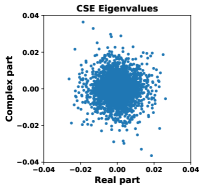
(a)

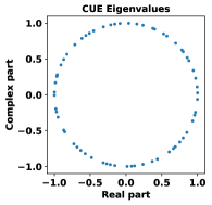
(b)

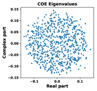
(c)

Figure 1: An example set of eigenvalues on the complex plane for (a) CSE (b) CUE and (c) COE.

A second step is to define a distance metric between two $\Omega$ distributions $\Omega^{N_{a}}$ and $\Omega^{N_{b}}$ generated according to Eq. 1 and corresponding to ensembles of matrix sizes $N_{a}$ and $N_{b}$, respectively. We define the distance metric as

$$D_{se}(N_{a},N_{b})=D_{KL}(\Omega^{N_{a}}||\Omega^{N_{b}})+D_{KL}(\Omega^{N_{b}}||\Omega^{N_{a}}),$$ (3)

where

$$D_{KL}(\Omega^{N_{a}}||\Omega^{N_{b}})=\sum_{k=1}^{K}\Omega^{N_{a}}_{k}\log_{2}(\Omega^{N_{a}}_{k}/\Omega^{N_{b}}_{k}).$$ (4)

The sum of two terms in Eq. (3) is due to the non-symetric nature of Eq. (4). Clearly, the new metric based on Eqs. (3) and (4) is rooted on the Kullbach-Leibler (KL) divergence [24, 25], although one should notice that we do not apply the new metric to probability distribution functions but to $\Omega$ distributions generated according to Eq. 1. $D_{se}(N_{a},N_{b})$ allows to assess how increasing network size, i.e. larger connectivity matrix, influences the approach to spectral ergodicity. In order to test our new method in the field of deep learning, instead of working on a specific architecture and learning algorithm, we use random matrices to mimic a generic ensemble of weight matrices, such as in feed-forward architectures, i.e., deep learning [12, 13] or in recurrent networks [26]. Using random matrices brings a distinct advantage of generalising the results for any architecture using a simple toy system and being able to enforce certain restrictions on the spectral radius. For example, applying a constraint on the spectral radius to unity, this simulates preventing vanishing or exploding gradient problems in training the network [17]. Circular random matrix ensembles serve this purpose well, where their eigenvalues lie on the unit circle in the complex plane. A typical weight matrix for a layer, $W$, in deep feed-forward multi-layer neural networks, is not square. In those cases one can proceed with the square matrix $W^{T}W$ to find the eigenvalue spectrum.

Implementation of parallel code generating circular random matrix ensembles [27, 28], using Mezzadri’s approach [29, 30], is utilized. Using circular ensembles circumvents the need for spectral unfolding [18]. Random seeds are preserved for each chunk from an ensemble, so that the results are reproducible both in parallel and serial runs [27]. Three different circular ensembles are generated.

Realisations for circular ensembles can be generated as follows. Consider a Hermitian matrix $H\in\mathbb{C}^{N\times N}$, in component form,

$$H_{ij}=\frac{1}{2}(a_{ij}+Ib_{ij}+a_{ji}-Ib_{ji}),$$

where $1\leq i,j\leq N$, and $a_{ij},b_{ij},a_{ji},b_{ji}\in\mathbb{G}$, i.e, they are elements of the set of independent identical distributed Gaussian random numbers sampled from a normal distribution and $I$ is the imaginary number.

The Circular Unitary Ensemble (CUE) is defined as

$$U=exp(\gamma_{i}I)\cdot v_{j}^{i},$$

$v_{i}$ is the $i$-th eigenvector of $H_{ij}$, where $\gamma_{i}\in[0,2\pi]$ is a uniform random number. The Circular Orthogonal Ensemble (COE) is dependent on CUE as follows,

$$O=U^{T}U.$$

The Circular Symplectic Ensemble (CSE) also depends on CUE,

$$S=(ZU^{T}Z)U,$$

where $S\in\mathbb{C}^{2N\times 2N}$, $Z\in\mathbb{R}^{2N\times 2N}$ a symplectic matrix obtained by the outer product of the $N\times N$ identity matrix with the unit antisymmetric $2\times 2$ matrix. In summary, $Z$ is formed by placing blocks of antisymmetric unit matrices of size $2\times 2$ over diagonals of $2N\times 2N$ matrix, and leaving off-diagonal elements zero.

Simulated circular ensembles consist of matrices of different sizes: $64,128,256,512,768,1024$ with ensemble size of $40$ each. Eigenvalues of all matrices lie within a unit circle on the complex plane. We see that typical eigenvalues for CSE are concentrated in a more dense region in Figure 1(a). Similarly, typical eigenvalues are shown in Figure 1(b) and Figure 1(c), for CUE and COE respectively. They are more spread for COE. In the case of CUE, all eigenvalues lie on the unit circle.

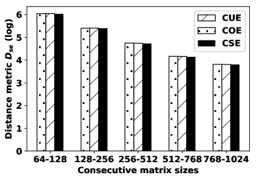
Figure 2: Distance metric for spectral ergodicity, $D_{se}(N_{j})$, for CUE, COE and CSE. Labels shows the consecutive sizes used in computing $D_{se}(N_{a})$ on the horizontal axis.

Approach to spectral ergodicity $D_{se}(N_{a},N_{b})$ for all circular ensembles is computed. Spectra are constructed via a histogram of arguments of eigenvalues, as they are complex, with a fixed binwidth over all ensembles. It is seen that results are robust against different binwidths.

As in Figure 2 where $D_{se}(N_{a},N_{b})$ distance is shown as a function of the matrix size, the surrogate weight matrices at fixed size of the ensembles, a consistent decrease in $D_{se}(N_{a},N_{b})$ with increasing matrix size is observed. This can be interpreted as spectral ergodicity being a property of deep neural networks; an ensemble here can be thought as the number of layers having fixed number of neurons at each layer, matrix size of $N$. With this fixed ensemble size, we observe that using larger sizes of hidden layers leads to spectral ergodicity faster.

Hence, $D_{se}(N_{a},N_{b})$ can help us to identify a lower bound on how large a layer to use in learning algorithms. One could identify an ensemble of architectures or different depths of layers, and construct an ensemble of weight matrices. An optimal combination of learning algorithm and architecture can be identified when spectral ergodicity is reached within a given threshold. This approach would save the practitioner both computation time and design effort.

COE and CSE ensembles produce smaller eigenvalues, with a spectral radius $\rho$, less than 0.2. This may generate a vanishing gradient issue in learning algorithms [17], however the elements, i.e. weights of COE and CSE matrices can be upscaled so that the maximal eigenvalue is 1, this numerical change will not change the generic behavior based on spectral ergodicity we have observed.

Using information-theoretic measures to understand deep learning has been recently explored [31]. In this framework, it is argued that the optimal architecture, number of layers and connection in each layer, can be determined via propagation of the mutual information (MI) between the layers. Even though, our new metric $D_{se}(N_{a},N_{b})$ is not formally a Kullbach-Leibler distance, so it is not an information metric, we can capture similar characteristics from the layers without the need of prior knowledge about the learning algorithm or the training data. Our approach only requires weight matrices.

Success of deep learning architectures is attributed to availability of large amounts of data and being able to train multiple layers at the same time [12, 13]. However, how this is possible from a theoretical point of view is not well established. We introduce quantification of spectral ergodicity for random matrices as a surrogate to weight matrices in deep learning architectures and argue that spectral ergodicity conceptually can improve our understanding about how these architectures perform learning with high accuracy. From a biological standpoint, our results also show that spectral ergodicity would play an important role in understanding synaptic matrices, as random matrices are used in understanding dynamics and memory in the brain as well [7, 8, 11].

We thank Christian Garbers for valuable discussion on circular statistics and code review. Ruben Foission and Marcel Reginatto for sharing their notes on spectral unfolding.

References

- Mehta [2004] M. L. Mehta, Random Matrices, Vol. 142 (Academic press, 2004).
- Edelman and Rao [2005] A. Edelman and N. R. Rao, Acta Numerica 14, 233 (2005).
- Mezzadri and Snaith [2005] F. Mezzadri and N. Snaith, Cambridge Univ Pr, (2005).
- Forrester [2010] P. J. Forrester, Princeton Univ Pr, (2010).
- Couillet and Debbah [2011] R. Couillet and M. Debbah, Princeton Univ Pr, (2011).
- Bai et al. [2014] Z. Bai, Z. Fang, and Y. Liang, Spectral Theory of Large Dimensional Random Matrices and Its Applications to Wireless Communications and Finance Statistics: Random Matrix Theory and its Applications (World Scientific Publishing Company, 2014).
- Rajan and Abbott [2006] K. Rajan and L. Abbott, Physical Review Letters 97, 188104 (2006).
- Aljadeff et al. [2015] J. Aljadeff, M. Stern, and T. Sharpee, Physical Review Letters 114, 088101 (2015).
- Parisi et al. [2015] G. I. Parisi, C. Weber, and S. Wermter, Frontiers in Neurorobotics 9, 3 (2015).
- Ahmadian et al. [2015] Y. Ahmadian, F. Fumarola, and K. D. Miller, Physical Review E 91, 012820 (2015).
- Rajan et al. [2016] K. Rajan, C. D. Harvey, and D. W. Tank, Neuron 90, 128 (2016).
- LeCun et al. [2015] Y. LeCun, Y. Bengio, and G. Hinton, Nature 521, 436 (2015).
- Bengio [2009] Y. Bengio, Foundations and Trends in Machine Learning 2, 1 (2009).
- Srivastava et al. [2014] N. Srivastava, G. E. Hinton, A. Krizhevsky, I. Sutskever, and R. Salakhutdinov, Journal of Machine Learning Research 15, 1929 (2014).
- Cerdà and Sintes [2005] J. J. Cerdà and T. Sintes, Biophysical Chemistry 115, 277 (2005).
- Süzen [2014] M. Süzen, Physical Review E 90, 032141 (2014).
- Pascanu et al. [2013] R. Pascanu, T. Mikolov, and Y. Bengio, ICML (3) 28, 1310 (2013).
- Haake [2013] F. Haake, Quantum Signatures of Chaos, Vol. 54 (Springer Science & Business Media, 2013).
- Peters and Klein [2013] O. Peters and W. Klein, Physical Review Letters 110, 100603 (2013).
- Jackson et al. [2001] A. Jackson, C. Mejia-Monasterio, T. Rupp, M. Saltzer, and T. Wilke, Nuclear Physics A 687, 405 (2001).
- Desjardins et al. [2010] G. Desjardins, A. Courville, Y. Bengio, P. Vincent, and O. Delalleau, in Proceedings of the Thirteenth International Conference on Artificial Intelligence and Statistics, Proceedings of Machine Learning Research, Vol. 9, edited by Y. W. Teh and M. Titterington (PMLR, Chia Laguna Resort, Sardinia, Italy, 2010) pp. 145–152.
- Mountain and Thirumalai [1989] R. D. Mountain and D. Thirumalai, The Journal of Physical Chemistry 93, 6975 (1989).
- Thirumalai et al. [1989] D. Thirumalai, R. Mountain, and T. Kirkpatrick, Physical Review A 39, 3563 (1989).
- Kullback and Leibler [1951] S. Kullback and R. A. Leibler, The Annals of Mathematical Statistics 22, 79 (1951).
- Bishop [2007] C. M. Bishop, Pattern Recognition and Machine Learning (Springer, 2007).
- Lukoševičius and Jaeger [2009] M. Lukoševičius and H. Jaeger, Computer Science Review 3, 127 (2009).
- Süzen [2017] M. Süzen, Python Random Matrix Tools (2017), https://pypi.python.org/pypi/bristol.
- Süzen et al. [2017] M. Süzen, C. Weber, and J. J. Cerdà, Dataset (2017), https://doi.org/10.5281/zenodo.822411.
- Mezzadri [2006] F. Mezzadri, Notices of AMS 54, 592 (2006).
- Berry and Shukla [2013] M. Berry and P. Shukla, New Journal of Physics 15, 013026 (2013).
- Tishby and Zaslavsky [2015] N. Tishby and N. Zaslavsky, Information Theory Workshop (ITW), IEEE , 1 (2015).