Simulating Wear
On Total Knee Replacements

Abstract

Wear on total knee replacements (TKRs) is an important criterion for their performance characteristics. Numerical simulations of such wear has seen increasing attention over the last years. They have the potential to be much faster and less expensive than the in vitro tests in use today. While it is unlikely that in silico tests will replace actual physical tests in the foreseeable future, a judicious combination of both approaches can help making both implant design and pre-clinical testing quicker and more cost-effective.

The challenge today for the design of simulation methods is to obtain results that convey quantitative information, and to do so quickly and reliably. This involves the choice of mathematical models as well as the numerical tools used to solve them. The correctness of the choice can only be validated by comparing with experimental results.

In this paper we present finite element simulations of the wear in TKRs during the gait cycle standardized in the ISO 14243-1 document, used for compliance testing in several countries. As the ISO 14243-1 standard is precisely defined and publicly available, it can serve as an excellent benchmark for comparison of wear simulation methods. Our novel contact algorithm works without Lagrange multipliers and penalty methods, achieving unparalleled stability and efficiency. We compare our simulation results with the experimental data from physical tests using two different actual TKRs, each test being performed three times. We can closely predict the total mass loss due to wear after five million gait cycles. We also observe a good match between the wear patterns seen in experiments and our simulation results.

1 Introduction

The wear between tibial plateau and femur component is one of the main limiting factors for the life-span of total knee replacements (TKRs). In the course of millions of gait cycles, the hard femur head grinds off small particles from the tibial plateau, which is usually made from relatively soft polyethylene (UHMWPE). Small microparticles start to migrate within the knee joint, leading to inflammation and eventually osteolysis (Gupta et al., 2007). In extreme cases, mechanical failure of (the surface of) the tibial plateau is observed.

To limit these risks various national guidelines require pre-clinical in vitro testing of the wear behavior of knee implants. These tests are performed by knee wear testing machines. The precise conditions are formulated in a series of documents published by the International Standards Organisation. We focus here on ISO 14243-1 (ISO, 2009), which describes testing conditions of a load-controlled testing gait cycle for normal walking. A wear test consists of five million such cycles, and of monitoring the mass loss of the tibial bearing component.

Performing such experimental tests is a cost-intensive task. The required five million cycles take about three months of time. Sometimes tests have to be aborted in mid way, because the initial positioning was not well chosen. (Indeed, the initial positioning of the femur and tibia with respect to each other is not precisely specified by ISO 14243-1.) Its determination remains an important open problem even for the designers of knee implants.

Computer simulations of these standardized tests can help to reduce costs and time-to-market. While simulations cannot replace the actual compliance tests, they can help to avoid some of the preliminary tests that need to be performed during the design phase of a new implant. In particular, numerical simulations can help to determine suitable initial configurations. With this information, the number of actual physical experiments is greatly reduced.

For these reasons, the numerical simulation of TKR wear behavior has seen increasing interest over the past years. Various finite element and rigid body models appear in the literature, all combining different contact formulations and wear laws. While some authors consider Archard’s wear law to be sufficient (O’Brien et al., 2013; Willing and Kim, 2009), others focus on developing more advanced laws to better capture the behavior of UHMWPE (Abdelgaied et al., 2011; O’Brien et al., 2014). Several groups use the ISO 14243 test family as a benchmark problem (O’Brien et al., 2012; Willing and Kim, 2009), but only the latter group uses the load-controlled variant 14243-1. Abdelgaied et al. (2011) and O’Brien et al. (2014) compare their findings with experimental results.

In this contribution we describe a new finite element model of two TKRs including the tibia plateau and femoral component. Following Abicht (2005); Willing and Kim (2009), we model both components as deformable objects, because numerical tests showed that surprisingly little run-time can be saved by keeping the femur rigid. We model the contact between the two objects exactly, with a surface–to–surface (mortar) discretization (Wohlmuth, 2011; Laursen, 2002) without recurse to any regularization parameter. The wear on the tibial plateau is described using Archard’s wear law. We compare the predicted wear patterns and total wear mass loss to values obtained by experimental testing, and observe a very good correspondence. In particular, the choice of the comparatively simple Archard’s law appears to be appropriate. More complicated models may be useful in the future, but need more experimental data to be justified.

Numerical wear testing involving deformable objects requires the solution of many contact problems, in particular if long-time wear, statistical effects, or shape-optimization is involved. Most articles mentioned above use commercial finite element software, which typically uses Lagrange multipliers or penalty approaches for the contact problems. The well-known drawbacks are additional degrees of freedom, artificial parameters, penalization errors, and instabilities. In contrast, our contact model uses a novel nonsmooth multigrid algorithm which solves the contact problems directly. This avoids all abovementioned drawbacks—instead, the solver is provably convergent, and as fast as solvers for linear elastic problems without contact (Gräser et al., 2009). We implemented the model in a C++ code based on the open-source Dune library (www.dune-project.org). The efficiency and stability of our algorithm allows to solve challenging wear simulations quickly and reliably.

2 Methods

We simulate the ISO 14243-1 testing cycle using a finite element model that includes both the femur component and the tibial inlay of the implant as deformable bodies. The two interact by a contact condition which we model using a surface–to–surface (mortar) contact discretization (Laursen, 2002; Wohlmuth, 2011). As TKRs are well lubricated inside the testing machine we assume the contact to be frictionless. The numerical code is our own research implementation based on the open-source finite element code Dune (Blatt et al., 2016; Bastian et al., 2010) (www.dune-project.org).

2.1 Finite Element Model

mesh		# elements	# vertices
Mebio 1	femur	13 824	4 633
	tibia	3 948	1 205
Mebio 2	femur	31 432	9 234
	tibia	81 400	17 445
Mebio 3	femur	184 526	42 750
	tibia	188 993	37 982
Genius Pro 1	femur	9 238	2 820
	tibia	4 720	1 496
Genius Pro 2	femur	33 864	8 745
	tibia	18 799	5 038
Genius Pro 3	femur	109 045	24 550
	tibia	121 548	26 484

Table 1: Mesh resolutions. For each of the two TKRs, meshes in three different resolutions were constructed.

We tested our simulation procedure with two implants which are sold commercially, and for which all geometry data and the original experimental results of the ISO 14243-1 compliance testing were gratefully made available to us by the manufacturer (aap Implantate GmbH).

These are a “Mebio 2015” (in the following: Mebio (QuestMed GmbH, 2015)) and a “Genius Pro (Fixed Bearing, PCL retaining)” (in the following Genius Pro (Endolab GmbH, 2011)). CAD data of the TKR volumes was available in Parasolid format. Tetrahedral volume meshes with different resolutions were constructed using ANSYS (ANSYS Inc., Canonsburg, PA) and the open source mesh generator gmsh (Geuzaine and Remacle, 2009). The meshes for the tibial component have between 5 000 and 120 000 elements, and 1 500 to 26 500 vertices for the Genius Pro implant, and between 4 000 and 190 000 elements (1 200 to 38 000 vertices) for the Mebio implant, see Table 1. Four-node tetrahedral finite elements were used for the discretization.

Figure 1: Meshes for femur component of Mebio implant

Figure 2: Meshes for tibial component of Mebio implant

Figure 3: Meshes for femur component of Genius Pro implant

Figure 4: Meshes for tibial component of Genius Pro implant

To simplify the mesh construction, the geometries of the implants was simplified slightly on their respective back sides. The geometric modifications did not involve areas close to the contact region. Geometric changes this far away from the contact surface do not have a relevant influence on the wear behavior. Figures 1 and 2 show the meshes used for the Mebio implant; Figures 3 and 4 the ones used for the Genius Pro implant.

We model the UHMWPE of the tibial inlay as well as the cobalt–chromium–molybdenum alloy of the femur component as homogeneous, isotropic, linear elastic materials. Material parameters are taken from (Abicht, 2005, p. 51). We use Young’s modulus $E=220$ GPa, Poisson ratio $\nu=0.31$ for the femur, and $E=1.1$ GPa, $\nu=0.42$ for the tibial inlay.

Figure 5: Boundary conditions during the gait cycle

Time-dependent boundary conditions are set as described by the ISO 14243-1 standard. The standard describes a single gait cycle by giving a table listing boundary values for 100 discrete time steps within one gait cycle. In particular, the femur component is rotated following its movement in a knee bend, and then fixed using a displacement condition on its back side. The boundary conditions for the tibial inlay are slightly more complicated (Figure 5):

• The main load is an axial force pushing the tibial side upwards against the femur component, with time-dependent values between $167.6\,\mathrm{N}$ and $2600\,\mathrm{N}$,

• a smaller force acts on the inferior side of the tibial inlay in anterior–posterior direction with values between $-265\,\mathrm{N}$ and $110\,\mathrm{N}$,

• an internal–external torque around the axis of the axial force is applied, with values between $-1\,\mathrm{Nm}$ and $6\,\mathrm{Nm}$.

Additionally, the inlay is kept in place by springs penalizing anterior–posterior displacement and internal–external rotation. Note that this testing cycle is load-controlled and no displacement boundary condition is applied to the tibial side at all. This results in rank-deficient system matrices, making the finite element system particularly challenging to solve.

For each of the 100 time steps that make up the gait cycle, we need to solve a linear contact problem. As our model does not include inertia or rate effects, the results of these 100 steps are independent of each other and can be computed in parallel using OpenMP.

To stay within the limits of linear elasticity we use separate reference configurations for each time step of the gait cycle. The displacement boundary condition describes a rigid body motion of the femur component. We apply this motion to the femur component, and use the result as the reference configuration for the femur. In this rotated configuration, the force boundary and contact conditions do not lead to large strains or displacements, and the use of linear elasticity is justified.

We model the contact between the two objects by a penalty-free surface–to–surface (mortar) finite element discretization as described in Wohlmuth and Krause (2003). Mortar discretizations avoid the unphysical stress oscillations that are known to occur in node-to-node contact methods (Wohlmuth, 2011). The method is parameter-free, meaning that there are no additional values that would need proper tuning to make the algorithm function properly. The resulting systems of equations are solved using a nonsmooth multigrid method (Gräser et al., 2009) together with the interior-point solver IPOpt (Wächter and Biegler, 2006), which is guaranteed to converge to the solution in all cases, without the need for artificial load stepping.

2.2 Wear and Grid Deformation

We use Archard’s wear law (Archard and Hirst, 1956) to model the wear on the tibial inlay. For each point on the contact surface, Archard’s law models the wear depth $l$ at that point. The wear depth $l$ at a time $t$ is given by

$$l(t)=k\int_{0}^{t}|p(t)v(t)|\,dt,$$

where $k$ is a material constant, $p$ is the contact pressure at this point, and $v$ is the relative velocity between the two objects. If $p$ is independent of time, and the sliding velocity is constant, then we obtain the formula

$$l=kps,$$

with the sliding distance $s$ typically seen in the literature. Total volume loss is computed as the integral of $l$ over the contact surface. Pressure $p$ and current velocity $v$ are computed from the finite element model. For the wear constant $k$ we chose the value $2.0\cdot 10^{-7}\textrm{mm}^{3}/\textrm{Nm}$, taken from O’Brien et al. (2014, model M1). This is an important point: we did not use the experimental data available to us to determine the important wear coefficient $k$.

Figure 6: Convergence of the total wear mass loss with smaller cycle steps for the Mebio (left) and Genius Pro (right) implants. The lines for 20k, 25k and 50k cycles per step are overlapping.

Even with a fast numerical solver, solving the 100 time steps for each of the 5 million gait cycles mandated by ISO 14243-1 is not possible. However, since Archard’s wear law does not directly depend on the wear history, we can extrapolate the wear values obtained for a single gait cycle over a larger number of cycles. We estimate the wear over $n_{\Delta}$ cycles by extrapolating the wear of a single gait cycle linearly, i.e., by multiplying $l$ by $n_{\Delta}$. To obtain a reasonable value for the cycle step size $n_{\Delta}$, we performed simulations on a single grid per implant and compared the total wear loss over time for different choices of $n_{\Delta}$ between $2\cdot 10^{4}$ and $2\cdot 10^{5}$. The results from Figure 6 show that a step size of $5\cdot 10^{4}$ cycles per step is a good choice for $n_{\Delta}$.

Linear extrapolation works over numbers of gait cycles that are not too large. However, when very large numbers of cycles are considered, the change in geometry needs to be taken into account. This change will be hardly noticable on the femur, but very relevant on the softer tibial inlay. Therefore, after each $n_{\Delta}$ gait cycles, we deform the tibial grid by adding the extrapolated wear depth in normal direction to the grid contact surface. From then on, this modified geometry is used as the reference configuration for the subsequent simulation steps. As the wear depth $l$ is small, adding it to the grid hardly influences the grid quality at all. To be on the safe side, after changing the grid boundary we also adjust the inner grid node positions by moving them according to the solution of a linear elastic problem for the tibial inlay with the wear depth $l$ as displacement boundary condition.

Combining finite element simulations, linear extrapolation, and grid deformation, we arrive at the following hybrid time-stepping method to compute long-time wear patterns and mass loss. Pick an extrapolation step size $n_{\Delta}$, and perform the following three steps:

1. Compute surface wear for a single gait cycle.

2. Multiply result by $n_{\Delta}$ to obtain the extrapolated values for $n_{\Delta}$ gait cycles.

3. Modify geometry using the extrapolated wear depth.

These three steps are repeated until the total number of gait cycles reaches 5 millions. The result is the total mass loss due to wear over time, and the wear patterns in the tibia that can be read off directly from the grid.

3 Results

The simulation results match the results of the experimental testing very well. Figure 7 shows the total mass loss due to wear after up to 5 million gait cycles for the two implant geometries. Three sets of experimental data are given for each implant, because the same in vitro experiment was repeated three times to get an idea of the overall variance of the measurements. For both implant types there are two sets of data that agree very well with each other, whereas the third one shows lower values.

The simulation predicts 98.31/81.04/53.13 mg of mass loss for the Mebio for the three grids, and 112.18/100.15/98.44 mg for the Genius Pro after 5 million cycles. The corresponding experimental results are in the range of 66.5–77.6 mg for the Mebio, and between 59.33–84.65 mg for the Genius Pro. We observe that mass loss for the Genius Pro implant appears to converge for increasing mesh resolution, whereas the corresponding number for the Mebio implant does not. This highlights the difficult nonlinear nature of the contact/wear problem.

We also observe that the experimental curves start with a steeper slope that flattens after about 1 million gait cycles, an effect that is not reproduced by the simulation. The presumed cause for this is that unused implants have a rougher surface, which becomes smoother after an initial number of cycles. Surface smoothness could be integrated easily into our model by using an iteration-dependent wear coefficient $k$. For simplicity, we have used the classical Archard’s law that assumes the wear constant $k$ to be fixed, because the overall effect seem to be negligeable.

Figures 8 and 9 show the simulated wear patterns for both implants. For the Mebio implant, sizes, shapes and positions of the wear marks match the corresponding experimental results very well, as can be seen in the overlay in Figure 10. Wear occurs on 12.5 – 15.6% of the proximal side of the tibial inlay in the simulation compared to 13.7 – 16.5% in the experiment. These values were computed by manually segmenting the wear marks, and counting pixels.

The experimental wear pattern of the Genius Pro implant shows several secondary wear marks near the border of the tibial plateau (Figure 11). These are typical for this type of implant, and they are caused by anterior–posterior translations in the swing phase. The numerical simulation does not show these marks; presumably a linearization effect. The main wear marks do not appear quite at the positions of the experimental ones. Wear occurs on approximately 10% of the surface in the simulation; on the experimental side the area is much larger (about 20%). From the distribution one can see that the numerical simulation does not resolve the increase of the wear area due to anterior–posterior movement.

In both cases, the experiments show two distinct depressions in the two main wear marks, separated by small ridges (Figure 13). This effect is not reproduced by the numerical algorithm.

The simulation also makes precise predictions about the wear depth at each point on the tibial surface. Figure 12 shows the deformed top surface of the tibial inlay after 5 million gait cycles. The vertical elevation has been stretched by a factor of $5$, to make the wear pattern more visible.

Figure 7: Wear mass loss for the Mebio (left) and Genius Pro (right) implants. The figure shows both experimental results taken at intervals of one million gait cycles and the simulation results. The geometry was adapted every $5\cdot 10^{4}$ gait cycles.

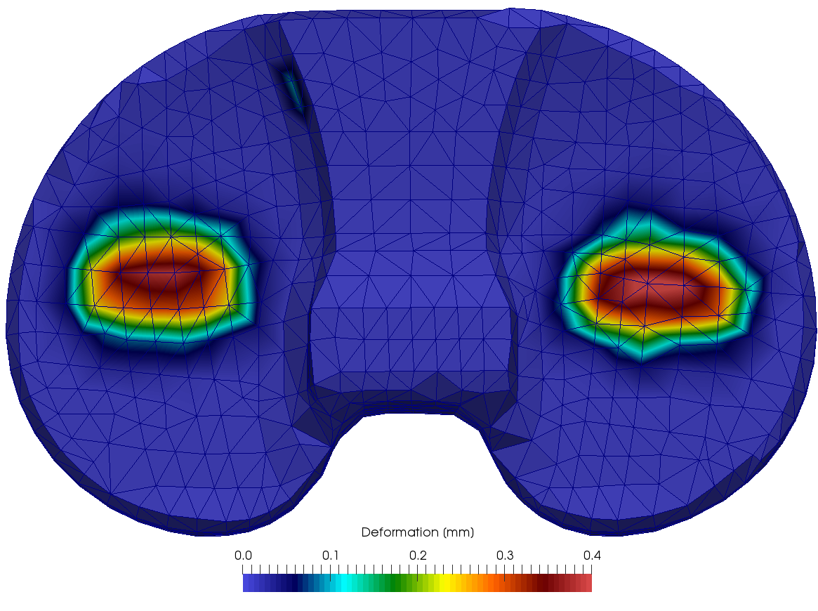
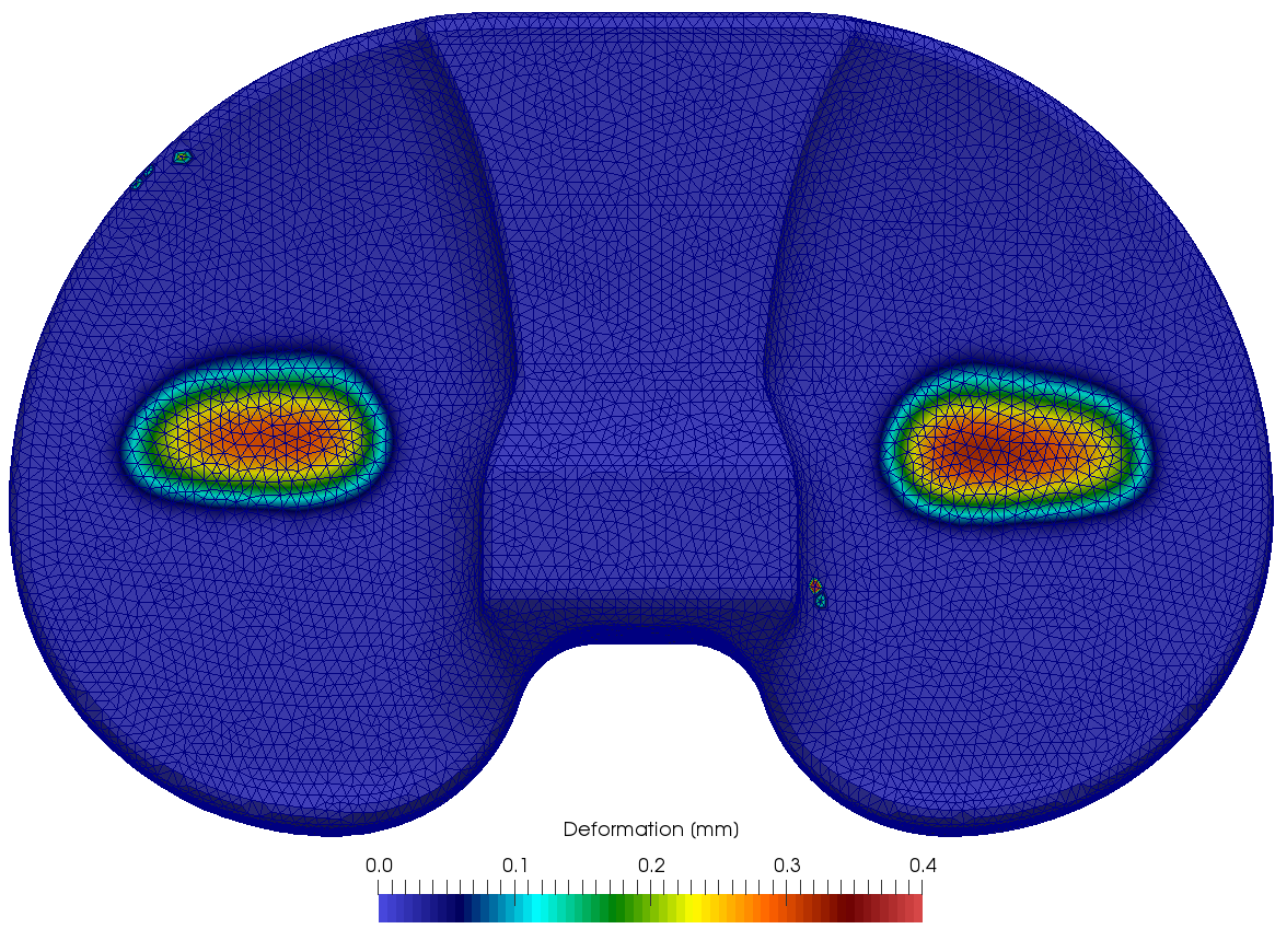
Figure 8: Spatial distribution of wear for the Mebio implant. Color denotes the wear depth.

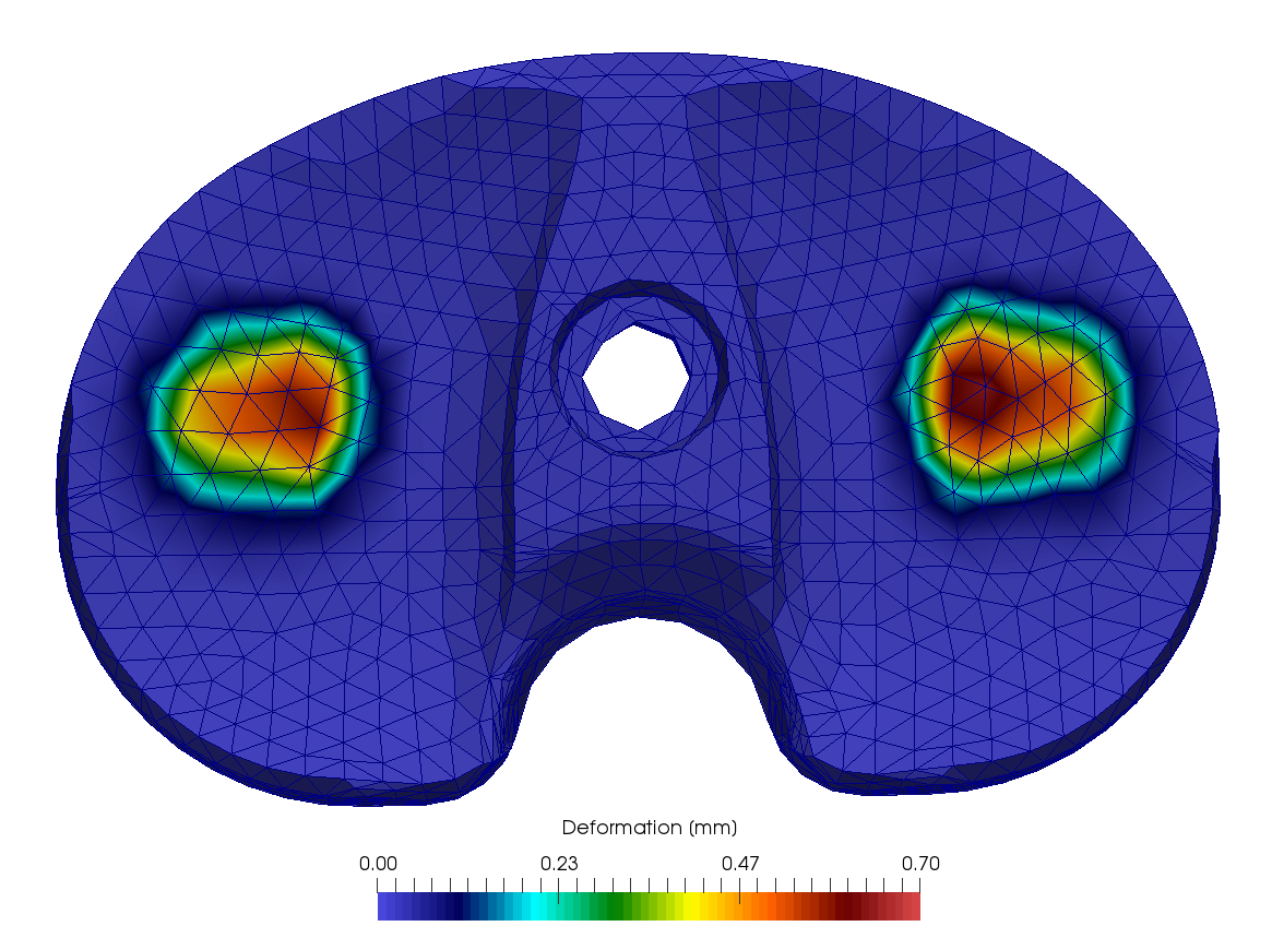
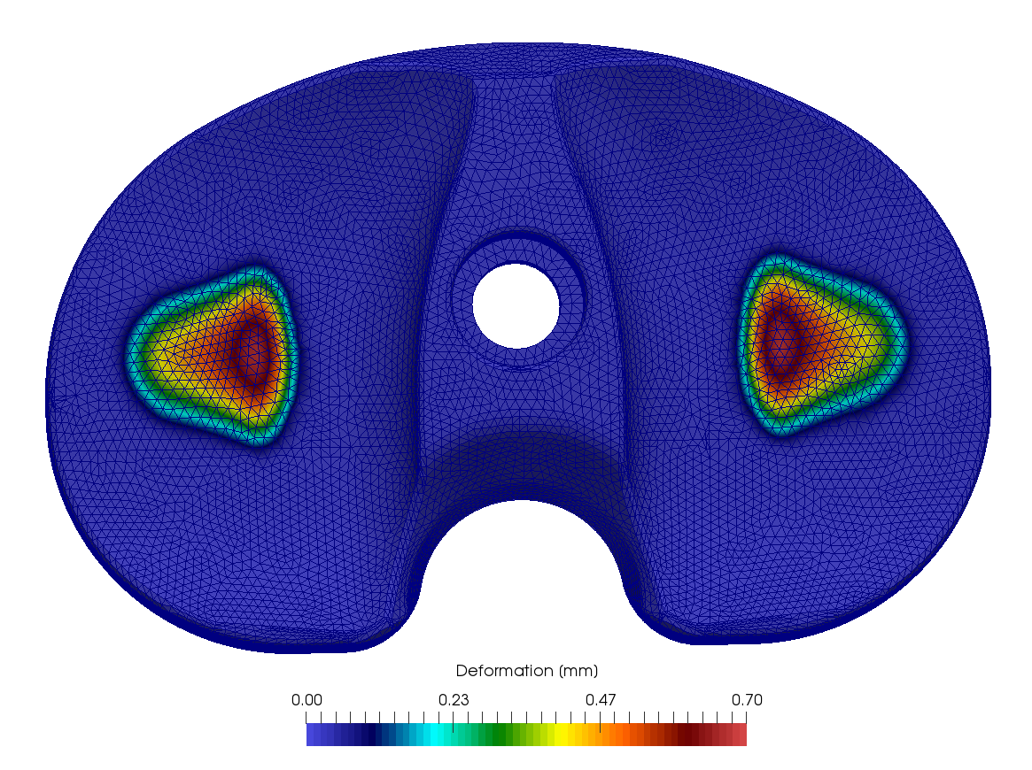
Figure 9: Spatial distribution of wear for the Genius Pro implant. Color denotes the wear depth.

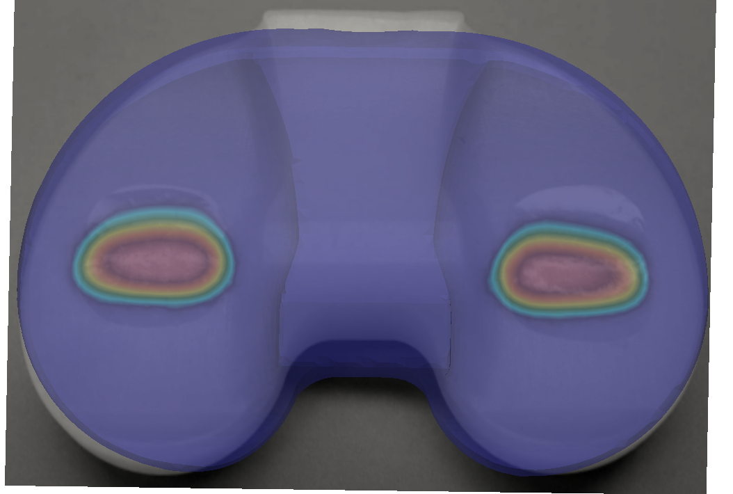
Figure 10: Overlay of simulated and experimental wear for Mebio implant after 5 million gait cycles

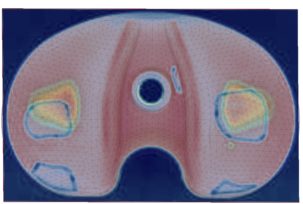
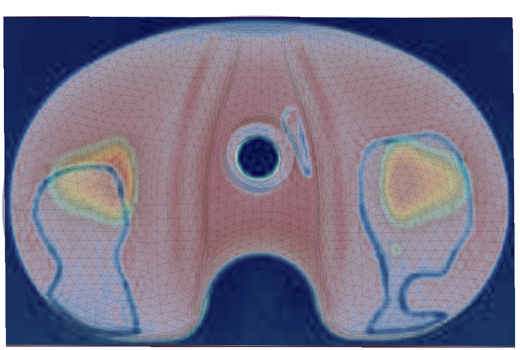
Figure 11: Overlay of simulated and experimental wear for Genius Pro implant after 5 million gait cycles. The wear marks on the edges of the implement are typical in this type. They are caused by anterior–posterior translations in the swing phase.

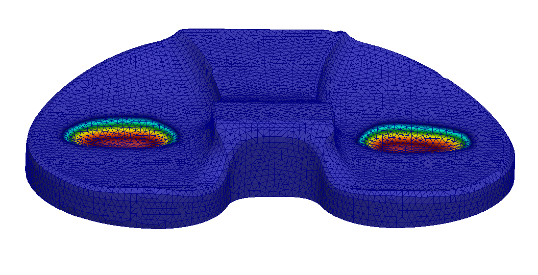
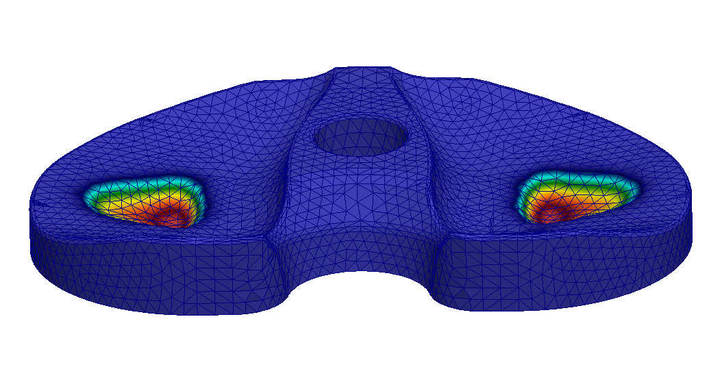
Figure 12: Tibial component of the Mebio (left) and Genius Pro (right) implants deformed by wear after 5 million simulated gait cycles. The deformation is scaled by a factor of $5$ to be better visible.

When using a single processor (Intel Xeon E5-2690, 2.9 GHz) the total simulation on medium-sized meshes with 12 to 14 thousand degrees of freedom in total took 22–30 hours. By far the majority of time was spent solving the contact problems. These problems were solved up to a relative accuracy of $10^{-8}$ for the displacement fields. More run-time can be saved when less accuracy is desired.

As the 100 contact problems of a single gait cycle can be computed independently from each other, it is straightforward to distribute them across several processors. The contact problems take the majority of the run-time, and therefore we expect almost linear scaling for up to 100 processors. Indeed, when repeating the simulations with 10 processors, the simulation took only between $2.7$ and $3.6$ hours. This is a speed-up of about 8.1–8.4 compared to the single-processor run.

4 Discussion

The results show that a numerical simulation can produce quantitative results of the wear on a TKR during an ISO 14243-1 testing cycle that are very close to the results obtained by actual experiments. Therefore, while numerical simulations are not yet reliable enough to completely replace in vitro pre-clinical testing, they nevertheless have the potential to reduce the number of tests in the design and pre-clinical phase, thereby reducing development costs and time-to-market.

As a particular example, note that the ISO 14243-1 document does not completely specify the initial mutual positioning and orientation of the femural and tibial TKR parts, because, by necessity, they are somewhat design-dependent. However, the initial positioning is something that even the manufacturer needs to determine by experimental testing. Therefore, occasionally tests need to be aborted, because faulty initial positioning will lead to artifacts like the wear marks near the circular hole seen in Figure 11. Here, numerical tests can be of great help, as they allow to cheaply check whether a given position is reasonable.

A standard ISO 14243-1 test simulating 5 million gait cycles takes about three month to complete. It is no particular challenge to construct finite element models that compute approximate wear marks and mass loss in less time than that. Nevertheless, it is desirable to have computer codes that are as fast as possible. The less time is needed for an in silico estimation of the wear behavior of a particular TKR, the better this information can be integrated into the design process. This is where our finite element model excels. A complete simulation with $n_{\Delta}=5\cdot 10^{4}$ takes only about 22–30 hours on a single processor. Even better, it scales almost linearly with the number of processors available (up to 100, because that is the number of substeps in the ISO 14243-1 gait cycle specification). As multi-processor machines have become cheap and commonplace over the years, it is no problem to obtain wear results for a complete test in even under half an hour. As a further bonus, our model is guaranteed to produce the result in all situations. No fine-tune of load-stepping parameters or similar human intervention is necessary. The algorithm runs completely autonomous. This saves precious human resources.

Furthermore, rapid numerical simulations open new possibilities even early in the design process. The impact of different variants of the implant shape on the wear behavior can be assessed without ever constructing a physical prototype. Modern mathematical techniques known as shape-optimization even allow to create optimal shapes automatically (Haslinger and Mäkinen, 2003; Willing and Kim, 2009). However, such methods can only be used in practice if a fast and reliable simulation tool for wear is available.

Archard’s wear law is the simplest one in a list of different models for mechanical wear. It is shown to give reasonably accurate results in many situations (Willing and Kim, 2009; O’Brien et al., 2013). Other wear laws try to take into account additional material properties such as cross-shearing, creep or dependency of the wear factor on contact pressure (Abdelgaied et al., 2011; Liu et al., 2010; O’Brien et al., 2014; Turell et al., 2003; Strickland et al., 2012), but none of them could be established as a standard so far. O’Brien et al. (2014) compare six different wear models, and obtain good results using Archard’s law.

We have found Archard’s law to be sufficient to obtain quantitative resuls of very good accuracy (Section 3). With this goal met, we can benefit from its advantages. The most important one is that Archard’s law contains only one unknown parameter, the wear coefficient $k$. We were able to pick a good parameter value from the literature, without any recourse to the TKR experimental data available to us. More precise values of the wear coefficient $k$ also depend on factors like the precise material and the method used to sterilize it. However, in production situations this is not a problem, as $k$ can be measured easily in separate experiments. More advanced wear laws would require additional parameters, which are in general not easy to obtain. Most likely, we would need additional TKR experimental data to determine material parameters by some form of regression analysis. Some laws additionally include internal states for which separate differential equations need to be solved. With such a wear law we would lose the ability to compute the hundred time steps of one gait cycle in parallel, sacrificing a lot of computational performance.

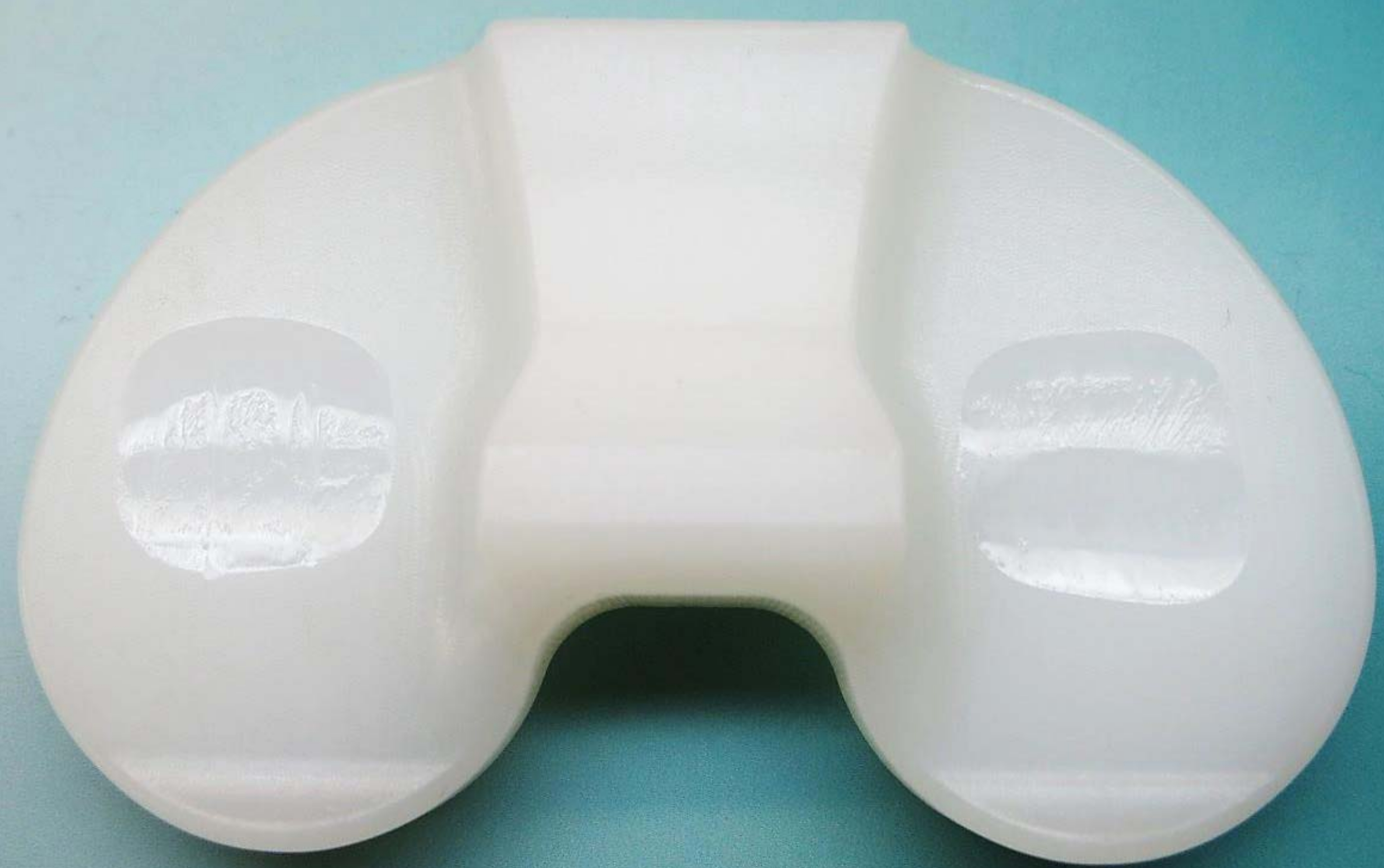
Figure 13: Experimental wear pattern on one of the samples of the Mebio implant. The separation in two valleys with a ridge in between can be seen.

In in vitro experiments it is frequently observed that the two main wear marks on the tibial plateau are not simple “holes”. Rather, they are typically formed from two or even three individual depressions, separated by ridges in medial–lateral direction (Figure 13). The origin of this special structure is unclear. Peculiarities of the testing gait cycle, friction effects, and plastic behavior of the UHMWPE are all plausible hypotheses. In our numerical experiments we have not ever been able to observe the lateral substructure. This does not rule out any possibilities, but it suggests that the load pattern by itself is not responsible. As the nature of this substructure is a practically relevant question, future research will have to try to capture it with more advanced models.

5 Conflict of interest statement

Ansgar Burchardt and Oliver Sander have no conflict of interest to disclose. Christian Abicht works for Questmed GmbH, an accredited test laboratory for physical testing of implants.

6 Acknowledgments

Ansgar Burchardt acknowledges support by the Project “05M2013–SOAK: Simulation des Abriebs von Knieimplantaten und Optimierung der Form zur patientengruppenspezifischen Abriebminimierung”, funded by the German Federal Ministry of Education and Research (BMBF).

References

-
Abdelgaied et al. (2011)
Abdelgaied, A., Liu, F., Brockett, C., Jennings, L., Fisher, J., Jin, Z., 2011.
Computational wear prediction of artificial knee joints based on a new wear
law and formulation. Journal of Biomechanics 44, 1108–1116.
URL https://dx.doi.org/10.1016/j.jbiomech.2011.01.027 - Abicht (2005) Abicht, C., 2005. Künstliche Kniegelenke nach dem Viergelenkprinzip: Konzeption, Design und tribologische Eigenschaften einer neuen Knieendoprothese mit naturnaher Gelenkgeometrie. Ph.D. thesis, Ernst-Moritz-Arndt-Universität Greifswald.
-
Archard and Hirst (1956)
Archard, J. F., Hirst, W., 1956. The wear of metals under unlubricated
conditions. Proceedings of the Royal Society of London A: Mathematical,
Physical and Engineering Sciences 236 (1206), 397–410.
URL https://dx.doi.org/10.1098/rspa.1956.0144 -
Bastian et al. (2010)
Bastian, P., Buse, G., Sander, O., 2010. Infrastructure for the coupling of
Dune grids. In: Proc. of ENUMATH 2009. Springer, pp. 107–114.
URL https://dx.doi.org/10.1007/978-3-642-11795-4_10 -
Blatt et al. (2016)
Blatt, M., Burchardt, A., Dedner, A., Engwer, C., Fahlke, J., Flemisch, B.,
Gersbacher, C., Gräser, C., Gruber, F., Grüninger, C., Kempf, D.,
Klöfkorn, R., Malkmus, T., Müthing, S., Nolte, M., Piatkowski, M.,
Sander, O., 2016. The distributed and unified numerics environment, version
2.4. Archive of Numerical Software 4 (100), 13–29.
URL https://dx.doi.org/10.11588/ans.2016.100.26526 - Endolab GmbH (2011) Endolab GmbH, 2011. Genius pro: Prüfbericht 42.110530.20.408, vom 11. 11. 2011 Geprüft bei Endolab GmbH, beauftragt von aap Implantate AG.
-
Geuzaine and Remacle (2009)
Geuzaine, C., Remacle, J.-F., 2009. Gmsh: A 3-d finite element mesh generator
with built-in pre- and post-processing facilities. International Journal for
Numerical Methods in Engineering 79 (11), 1309–1331.
URL https://dx.doi.org/10.1002/nme.2579 -
Gräser et al. (2009)
Gräser, C., Sack, U., Sander, O., 2009. Truncated nonsmooth Newton
multigrid methods for convex minimization problems. In: Domain Decomposition
Methods in Science and Engineering XVIII. Vol. 70 of Lecture Notes in
Computational Science and Engineering. Springer, pp. 129–136.
URL https://dx.doi.org/10.1007/978-3-642-02677-5_12 -
Gupta et al. (2007)
Gupta, S. K., Chu, A., Ranawat, A. S., Slamin, J., Ranawat, C. S., 2007. Review
article: Osteolysis after total knee arthroplasty 22, 787–799.
URL https://dx.doi.org/10.1016/j.arth.2007.05.041 - Haslinger and Mäkinen (2003) Haslinger, J., Mäkinen, R., 2003. Introduction to Shape Optimization: Theory, Approximation, and Computation. SIAM.
- ISO (2009) ISO, 2009. ISO 14243-1: Implants for surgery – Wear of total knee-joint prostheses – Part 1: Loading and displacement parameters for wear-testing machines with load control and corresponding environmental conditions for test. International standard.
- Laursen (2002) Laursen, T., 2002. Computational Contact and Impact Mechanics. Springer.
-
Liu et al. (2010)
Liu, F., Galvin, A. L., Jin, Z., Fisher, J., 2010. A new formulation for the
prediction of polyethylene wear in artificial hip joints. Proceedings of the
Institution of Mechanical Engineers Part H Journal of Engineering in Medicine
225 (1), 16–24.
URL https://dx.doi.org/10.1243/09544119JEIM819 -
O’Brien et al. (2012)
O’Brien, S., Luo, Y., Wu, C., Petrak, M., Bohm, E., Brandt, J.-M., 2012.
Prediction of backside micromotion in total knee replacements by finite
element simulation. Proceedings of the Institution of Mechanical Engineers,
Part H: Journal of Engineering in Medicine 226 (3), 235–245.
URL https://dx.doi.org/10.1177/0954411911435593 -
O’Brien et al. (2013)
O’Brien, S., Luo, Y., Wu, C., Petrak, M., Bohm, E., Brandt, J.-M., 2013.
Computational development of a polyethylene wear model for the articular and
backside surfaces in modular total knee replacements. Tribology International
59, 284–291.
URL https://dx.doi.org/10.1016/j.triboint.2012.03.020 -
O’Brien et al. (2014)
O’Brien, S. T., Bohm, E. R., Petrak, M. J., Wyss, U. P., Brandt, J.-M., 2014.
An energy dissipation and cross shear time dependent computational wear model
for the analysis of polyethylene wear in total knee replacements. Journal of
Biomechanics 47, 1127–1133.
URL https://dx.doi.org/10.1016/j.jbiomech.2013.12.017 - QuestMed GmbH (2015) QuestMed GmbH, 2015. Mebio: Prüfbericht TR15–046, vom 18. 5. 2015. Geprüft bei QuestMed GmbH, beauftragt von aap Implantate AG.
-
Strickland et al. (2012)
Strickland, M. A., Dressler, M. R., Taylor, M., 2012. Predicting implant
UHMWPE wear in-silico: A robust, adaptable computational–numerical
framework for future theoretical models. Wear 274–275, 100–108.
URL https://dx.doi.org/10.1016/j.wear.2011.08.020 -
Turell et al. (2003)
Turell, M., Wang, A., Bellare, A., 2003. Quantification of the effect of
cross-path motion on the wear rate of ultra-high molecular weight
polyethylene. Wear 255 (7–12), 1034–1039.
URL https://dx.doi.org/10.1016/S0043-1648(03)00357-0 -
Wächter and Biegler (2006)
Wächter, A., Biegler, T. L., 2006. On the implementation of an
interior-point filter line-search algorithm for large-scale nonlinear
programming. Mathematical Programming 106 (1), 25–57.
URL https://dx.doi.org/10.1007/s10107-004-0559-y -
Willing and Kim (2009)
Willing, R., Kim, I. Y., 2009. Three dimensional shape optimization of total
knee replacements for reduced wear. Structural and Multidisciplinary
Optimization 38 (4), 405–414.
URL https://dx.doi.org/10.1007/s00158-008-0281-0 -
Wohlmuth (2011)
Wohlmuth, B., 2011. Variationally consistent discretization schemes and
numerical algorithms for contact problems. Acta Numerica 20, 569–734.
URL https://dx.doi.org/10.1017/S0962492911000079 -
Wohlmuth and Krause (2003)
Wohlmuth, B. I., Krause, R. H., 2003. Monotone multigrid methods on nonmatching
grids for nonlinear multibody contact problems. SIAM Journal on Scientific
Computing 25 (1), 324–347.
URL https://dx.doi.org/10.1137/S1064827502405318