Fluctuations in an established transmission in the presence of a complex environment

Abstract

In various situations where wave transport is preeminent, like in wireless communication, a strong established transmission is present in a complex scattering environment. We develop a novel approach to describe emerging fluctuations, which combines a transmitting channel and a chaotic background in a unified effective Hamiltonian. Modeling such a background by random matrix theory, we derive exact non-perturbative results for both transmission and reflection distributions at arbitrary absorption that is typically present in real systems. Remarkably, in such a complex scattering situation, the transport is governed by only two parameters: an absorption rate and the ratio of the so-called spreading width to the natural width of the transmission line. In particular, we find that the established transmission disappears sharply when this ratio exceeds unity. The approach exemplifies the role of the chaotic background in dephasing the deterministic scattering.

I Introduction

In many applications ranging from electronic mesoscopic or quantum devices Beenakker (1997); Alhassid (2000); Mello and Kumar (2004) to telecommunication or wireless communication Tulino and Verdú (2004); Couillet and Debbah (2011), transmission and transport are the main focus of studies. Here, either the system or its excitation is designed to give a high transmission at the working energy (or frequency) ${\varepsilon_{0}}$. To guarantee the functionality of such devices, fluctuations in transmission induced by a complex environment are of crucial interest. Such variations might be introduced by uncertainties of the production process of electronic devices or by real-life changing environment like in wireless communication. In the latter case, e.g., one is interested in a stable communication that has strong transmission guaranteeing large signal to noise ratios as well as high data transfer rates Gesbert et al. (2000); Matthaiou et al. (2010). This is often implemented via multiple-input multiple-output (MIMO) systems Biglieri et al. (2007); Bliss and Govindasamy (2013); Karadimitrakis et al. (2016), which control the excitations thus giving rise to a special basis, where an established transmission is induced at ${\varepsilon_{0}}$. In electronic devices like quantum dots or wells, similar established transmission is put forward in the design of the system and placement of the leads Maryenko et al. (2012).

The analysis of complex quantum or wave systems often relies on predictions obtained for fully chaotic dynamics  Mello and Kumar (2004); Haake (2001). Random matrix theory (RMT) has proved to be extremely successful in describing universal wave phenomena in such systems Mehta (2004); Guhr et al. (1998). The canonical examples are spectral and wave function statistics, including their many experimental verifications Stöckmann (2007). When combined with the resonance scattering formalism Mahaux and Weidenmüller (1969), RMT offers a powerful approach Verbaarschot et al. (1985); Sokolov and Zelevinsky (1989); Fyodorov and Sommers (1997) to describe universal statistical fluctuations in scattering, see Mitchell et al. (2010); Fyodorov and Savin (2011) for recent reviews. The approach is also flexible in incorporating real world effects, like finite absorption, providing the non-perturbative theory Fyodorov et al. (2005); Kumar et al. (2013) to account for statistical properties of complex impedances Hemmady et al. (2005, 2006), transmission and reflection coefficients Kuhl et al. (2005a, b) observed in various microwave cavity experiments Dietz et al. (2010); Kuhl et al. (2013); Gradoni et al. (2014). From the theoretical side, non-universal aspects related to a deterministic part in scattering are usually removed from the very beginning by means of a certain procedure Engelbrecht and Weidenmüller (1973), yielding a new scattering matrix which becomes diagonal on average Verbaarschot et al. (1985). This, however, cannot be applied in the present case where fluctuations in a transmitting channel, characterised by the essentially non-diagonal deterministic $S$ matrix, are the main point of interest.

In this work, we propose a non-perturbative approach to quantify fluctuations in the established transmission mediated by a single energy level that is coupled to a complex environment modeled by RMT. The model in its original formulation goes back to nuclear physics Bohr and Mottelson (1969), giving rise to the well-known formalism of the strength function that has a rich history of various applications Harney et al. (1986); Sokolov and Zelevinsky (1997); Gu and Weidenmüller (1999); Savin and Sommers (2003); Sokolov (2010); Zelevinsky and Volya (2016). Nevertheless, a complete characterisation of fluctuations in the transmission for such a model in terms of its distribution function has not been reported in the literature so far and will be presented below.

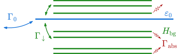
Figure 1: Schematic drawing of the model Hamiltonian. The single level ${\varepsilon_{0}}$ is coupled to scattering channels and a chaotic background $H_{\mathrm{bg}}$, leading to decay rates ${\Gamma_{0}}$ and ${\Gamma_{\downarrow}}$, respectively. Note that although the background states are not connected to the channels directly, they may have uniform broadening $\Gamma_{\mathrm{abs}}$ to account for homogeneous dissipation.

In the next section II, we introduce the model in detail, see Fig. 1 for an illustration. Section III provides the derivation of the exact RMT expressions for the transmission distribution, which is the main goal of this paper, first for the ideal case of zero absorption and then in the general case of arbitrary absorption. To complete the description of scattering, we address the distribution of reflections in Sec. IV, and then summarize with the conclusion and outlook. Further details on numerical implementations as well as an extension to incorporate losses on the single level, responsible for the established transport, are given in two appendices. In all cases, a good agreement between the exact analytical results and numerical simulations with random matrices is found.

II Scattering setup

The scattering problem in question is schematically represented by Fig. 1. We consider a two-port setup, which is typical for many experimental realisations, and assume that an established transmission between two channels occurs through a single resonance characterised by energy ${\varepsilon_{0}}$ and width ${\Gamma_{0}}$. This resonance state, which is often referred to as a doorway state Sokolov and Zelevinsky (1997, 1992), is coupled to a background Hamiltonian that represents influences of a complex environment. Due to a coupling to surrounding complicated states, the transmission channel spreads over the background with a rate given by the so-called spreading width ${\Gamma_{\downarrow}}$. The competition between the two decay mechanism is naturally controlled by the ratio

$$\eta={\Gamma_{\downarrow}}/{\Gamma_{0}}$$ (1)

between the spreading and escape widths.

We restrict our consideration to systems invariant under time-reversal, which is the case most relevant experimentally. Following Mehta (2004); Stöckmann (2007), we can then model the chaotic background by a random matrix drawn from the Gaussian orthogonal ensemble (GOE). Additionally, we assume that the background states may have uniform broadening to account for possible homogeneous absorption in the environment. The exact RMT results for the distribution functions derived below are non-perturbative and valid at any $\eta$ and arbitrary absorption.

II.1 Effective Hamiltonian approach

The scattering approach based on the effective non-Hermitian Hamiltonian Mahaux and Weidenmüller (1969); Sokolov and Zelevinsky (1989); Fyodorov and Savin (2011) is well adapted to treat both transport and spectral characteristics on equal footing. Neglecting global phases due to potential scattering, the scattering matrix $S$ can be written as follows

$$S(E)=1-iA^{T}\frac{1}{E-\mathcal{H}_{\mathrm{eff}}}A\,,$$ (2)

where $A$ is the energy-independent matrix of the coupling amplitudes between the channel and internal states, and

$$\mathcal{H}_{\mathrm{eff}}=H-\frac{i}{2}AA^{T}$$ (3)

defines the effective Hamiltonian of the open system. The Hermitian part $H$ corresponds to the Hamiltonian of the closed system, whereas the anti-Hermitian part accounts for finite lifetimes of resonances (eigenvalues of $\mathcal{H}_{\mathrm{eff}}$). The factorised structure of the latter ensures the unitarity of $S$ (at real scattering energy $E$). For systems invariant under time-reversal, $H$ and $A$ can be chosen as real, thus $S$ is a symmetric matrix.

We begin with quantifying a stable transmission between two channels in a “clean” system and consider a single level without any chaotic background. This amounts to setting above $H={\varepsilon_{0}}$ and $A=(a\ b)$, with two real parameters $a$ and $b$ determining the strength of coupling to the channels. The $S$ matrix elements are then given by a multichannel Breit-Wigner formula Mahaux and Weidenmüller (1969)

$$S(E)=1-\frac{i}{E-{\varepsilon_{0}}+(i/2){\Gamma_{0}}}\left(\begin{matrix}a^{2}&ab\\ ab&b^{2}\end{matrix}\right),$$ (4)

where the width ${\Gamma_{0}}$ is given by the sum

$${\Gamma_{0}}=a^{2}+b^{2}$$ (5)

of the partial decay widths. The peak transmission is achieved at the scattering energy $E={\varepsilon_{0}}$. The $S$ matrix evaluated at this point can be parameterised as follows

$$S_{0}=\left(\begin{matrix}-r_{0}&t_{0}\\ t_{0}&r_{0}\end{matrix}\right),$$ (6)

with the reflection and transmission amplitudes being

$$r_{0}=\frac{a^{2}-b^{2}}{{\Gamma_{0}}}\,,\qquad t_{0}=-\frac{2ab}{{\Gamma_{0}}}\,.$$ (7)

In view of Eq. (5), they satisfy the flux conservation $r_{0}^{2}+t_{0}^{2}=1$. Thus, we can express the scattering observables in terms of the experimentally measurable quantities: ${\varepsilon_{0}}$, ${\Gamma_{0}}$, and the transmission coefficient of the simple mode

$$T_{0}\equiv t_{0}^{2}=1-r_{0}^{2}\,.$$ (8)

In order to incorporate a complex environment acting on the transmission state, we follow the spreading width model Bohr and Mottelson (1969); Sokolov and Zelevinsky (1997) and represent the Hamiltonian as follows

$$H=\left(\begin{matrix}{\varepsilon_{0}}&\vec{V}^{T}\\ \vec{V}&H_{\mathrm{\,bg}}^{\mathrm{(goe)}}\end{matrix}\right).$$ (9)

Here, $H_{\mathrm{\,bg}}^{\mathrm{(goe)}}$ stands for the background Hamiltonian modelled by a random GOE matrix of size $N$, whereas vector $\vec{V}^{T}=(V_{1},\dots,V_{N})$ is responsible for coupling to the background. The elements of $\vec{V}$ can be chosen as real fixed or random mutually independent Gaussian variables with zero mean and a given second moment $\langle{V^{2}}\rangle$. By virtue of the invariance of the GOE with respect to basis rotations, the two choices become equivalent in the RMT limit of $N\gg 1$, with the obvious correspondence $V^{2}=\frac{1}{N}\|\vec{V}\|^{2}=\langle{V^{2}}\rangle$. For the sake of simplicity, we will assume $\vec{V}$ fixed in the following.

Neglecting a direct coupling of the GOE states to the channels, the coupling matrix $A$ takes the special form

$$A^{T}=\left(\begin{array}[]{cccc}a&0&\cdots&0\\ b&0&\cdots&0\end{array}\right).$$ (12)

As a result, one can easily find using Schur’s complement that the $S$ matrix retains the same structure of Eq. (4), where the following substitution is to be made

$$\frac{1}{E-{\varepsilon_{0}}+(i/2){\Gamma_{0}}}\to\frac{1}{E-{\varepsilon_{0}}+(i/2){\Gamma_{0}}-g(E)}$$ (13)

and the scalar function $g(E)$ is defined by

$$g(E) =\vec{V}^{T}\frac{1}{E-H_{\mathrm{\,bg}}^{\mathrm{(goe)}}}\vec{V}.$$ (14)

This is the so-called strength function Bohr and Mottelson (1969). By construction, it has the meaning of the local Green’s function of the complex background Fyodorov and Savin (2004), characterising its spectral properties. When averaged over this fine energy structure, the scattering amplitudes acquire an extra damping

$${\Gamma_{\downarrow}}{}=2\pi V^{2}/\Delta$$ (15)

in addition to ${\Gamma_{0}}$. The spreading width (15) is simply Fermi’s golden rule expressing the rate of decay into the “sea” of background states, the density of which is determined by the mean level spacing $\Delta$ Bohr and Mottelson (1969); Sokolov and Zelevinsky (1997).

II.2 $S$ matrix fluctuations

We are interested in fluctuations in scattering at the resonance energy ${\varepsilon_{0}}$. The $S$ matrix at this point can be represented in the following convenient form

$$S\equiv S({\varepsilon_{0}}{})=1-\frac{1}{1+i\eta K}(1-S_{0}),$$ (16)

where $\eta$ is given by Eq. (1) and we have introduced

$$K\equiv\frac{2}{{\Gamma_{\downarrow}}}g({\varepsilon_{0}}{})=\frac{\Delta}{\pi V^{2}}\vec{V}^{T}\frac{1}{{\varepsilon_{0}}-H_{\mathrm{\,bg}}^{\mathrm{(goe)}}}\vec{V}.$$ (17)

This quantity plays the role of the Wigner reaction matrix associated with scattering on the background [cf. Eq. (20) below]. Without loss of generality, we may let ${\varepsilon_{0}}$ be the centre of the semicirle law determining the mean density of the background states. With the definition $\Delta^{-1}=-(1/\pi)\mathrm{Im}\left\langle\mathrm{tr}({\varepsilon_{0}}+i0-H_{\mathrm{\,bg}}^{\mathrm{(goe)}})^{-1}\right\rangle$, one readily finds the average value $\langle{K}\rangle=-i$, resulting in

$$\left\langle{S}\right\rangle=\frac{\eta}{1+\eta}+\frac{1}{1+\eta}S_{0}$$ (18)

for the average $S$ matrix. This expression shows that $\eta$ controls the weight between the equilibrated and deterministic parts in scattering, which are given by the first and second terms in Eq. (18), respectively.

The average $S$ matrix is clearly non-diagonal because of channel mixing induced by $S_{0}$. Usually, the starting point of RMT applications to scattering  Verbaarschot et al. (1985); Fyodorov and Savin (2011) consists in eliminating such direct processes by means of a special similarity transform Engelbrecht and Weidenmüller (1973); Nishioka and Weidenmüller (1985). In the present case, however, this would remove the effect we are after. For similar reasons, one cannot use recent exact results Kumar et al. (2013); Nock et al. (2014) for the distribution of off-diagonal $S$ matrix elements (derived assuming a diagonal $\langle{S}\rangle$). In contrast, the obtained representation (16) enables us to solve the problem in its full generality by applying the non-perturbative theory for the local Green’s function, $K$, developed by Fyodorov, Sommers and one of the present authors in Fyodorov and Savin (2004); Savin et al. (2005); Fyodorov et al. (2005).

II.3 Background as a source of dephasing

It is instructive to give a physical interpretation to the above results in terms of the interference between the two scattering phases, the constant one due to the direct transmission and the random one induced by the chaotic background.

The deterministic part of the scattering matrix, $S_{0}$, can be brought to the diagonal form $O_{\varphi}^{T}S_{0}O_{\varphi}=\mathrm{diag}(-1,1)$ by an orthogonal matrix $O_{\varphi}$ that corresponds to a rotation by the angle $\varphi=\arctan\frac{t_{0}}{1+r_{0}}$. This angle expresses the degree of channel non-orthogonality due to the non-diagonal $A^{T}A$. By construction, the same transformation diagonalizes the full $S$ matrix (16), yielding

$$S=O_{\varphi}\mathrm{diag}(-S_{\mathrm{bg}},1)O_{\varphi}^{T},$$ (19)

where $S_{\mathrm{bg}}$ stands for the background contribution

$$S_{\mathrm{bg}}=\frac{1-i\eta K}{1+i\eta K}$$ (20)

into the full scattering process. Expression (20) is a usual form for the elastic (single-channel) scattering in open chaotic systems Verbaarschot et al. (1985); Sokolov and Zelevinsky (1989), with $\eta$ now playing the role of a degree of system openness. The resulting scattering pattern is therefore due to the interference between the deterministic phase $\varphi$ and the random phase $\theta=\mathrm{arg}(S_{\mathrm{bg}})$, the distribution of which is well-known Friedman and Mello (1985); Savin et al. (2001).

The model exemplifies the chaotic background as a natural source of dephasing in scattering processes (see also the relevant discussion in Sokolov (2010)). In contrast to two other dephasing models Büttiker (1986); Brouwer and Beenakker (1997), our formulation is very flexible in accommodating physically relevant properties of complex environments. In particular, homogeneous losses can be easily taken into account by uniform broadening $\Gamma_{\mathrm{abs}}$ of the background states. Operationally, such a damping is equivalent to the purely imaginary shift ${\varepsilon_{0}}{}+(i/2)\Gamma_{\mathrm{abs}}$ in the Green’s function (17) Savin and Sommers (2003). As a result, the latter becomes complex,

$$K=u-iv,$$ (21)

with the negative imaginary part, $v>0$ (the local density of states) Fyodorov and Savin (2004). The universal statistical properties of mutually correlated random variables $u$ and $v$ are solely determined by the (dimensionless) absorption rate

$$\gamma=2\pi\Gamma_{\mathrm{abs}}/\Delta.$$ (22)

Their joint distribution function is known exactly Savin et al. (2005); Fyodorov et al. (2005) and will be applied below to study fluctuations of $S$.

III Transmission distribution

It is convenient to define the re-scaled transmission coefficient $T=|S_{12}|^{2}/T_{0}$, expressed in the units of the peak transmission in the “clean” system. We now derive the exact results for the transmission distribution function

$$\mathcal{P}_{\gamma}(T)=\left\langle\delta(T-|S_{12}|^{2}/T_{0})\right\rangle,$$ (23)

first for the ideal case of the stable background ($\gamma=0$) and then for the general case of finite absorption.

III.1 Stable chaotic background

In the case of zero absorption, $K=u$ is real so the transmission coefficient is found from Eq. (16) as follows

$$T=\frac{1}{1+\eta^{2}u^{2}}.$$ (24)

The random variable $u$ is known Mello (1995); Fyodorov and Savin (2004) to have the standard Cauchy distribution. This stems from the fact that the scattering phase $\theta$, see Eq. (20), is distributed uniformly at special coupling $\eta=1$ not (a). The transmission distribution (23) follows then by a straightforward integration:

$$\mathcal{P}_{0}(T) =\int\limits_{-\infty}^{\infty}\frac{du}{\pi}\frac{1}{1+u^{2}}\delta\left(T-\frac{1}{1+\eta^{2}u^{2}}\right)$$

$$=\frac{1}{\pi\sqrt{T(1-T)}}\frac{\eta}{1+(\eta^{2}-1)T},$$ (25)

for $0\leq{T}\leq{1}$. The corresponding cumulative distribution function is given by

$$\mathcal{N}_{0}(T)=1-\frac{2}{\pi}\arctan\left(\frac{1}{\eta}\sqrt{\frac{1-T}{T}}\right).$$ (26)

Both functions are represented on Fig. 2

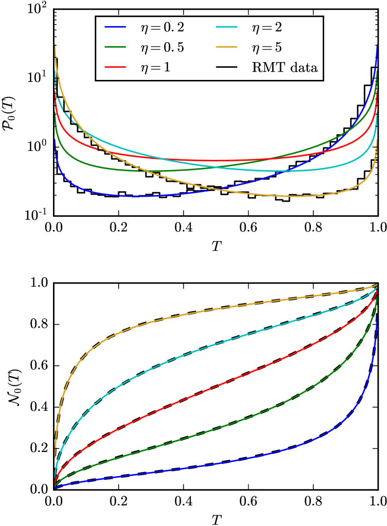
Figure 2: (color online). Transmission distribution for a stable chaotic background. The probability density (top) and cumulative distribution function (bottom) are shown at several values of the coupling parameter $\eta=0.2,0.5,1,2,5$. The solid curves stand for the analytical results (25) and (26). The histograms correspond to numerical simulations with $5{\times}10^{4}$ realizations of random $200\times 200$ GOE matrices. The data are shown only for $\eta=0.2$ and $5$, the agreement for the other values being similar. The numerics for the cumulative distribution (bottom, dashed lines) is indistinguishable from the theory within the linewidth.

The distribution (25) has a bi-modal shape with a square-root singularity at both edges, which is typical for transmission problems Beenakker (1997). The mean value is readily found to be $\langle{T}\rangle=(1+\eta)^{-1}$, in agreement with the general result (18), and the transmission variance reads

$$\langle{T^{2}}\rangle-\langle{T}\rangle^{2}=\frac{\eta}{2(1+\eta)^{2}}.$$ (27)

The background coupling, $\eta$, controls the weight of the distribution that is concentrated near $T\sim 1$ or $T\sim 0$ at small or large $\eta$, respectively. It becomes symmetric at $\eta=1$, with the variance attaining its maximum value. Further increase of $\eta$ leads to a sharp redistribution towards low transmission. For applications, this sets the limit $\eta=1$ on coupling for reliable signal transmission.

Figure 2 illustrates the above discussion and results. In order to check the validity of the predictions we present them together with numerical data from RMT simulations based on $5{\times}10^{4}$ realizations of $H_{\mathrm{\,bg}}^{\mathrm{(goe)}}$ blocks of size $200\times 200$. The parameters $a,b,V$, see Eqs. (7)–(9), are chosen to give $T_{0}=0.8$ and the various $\eta$ values. (For simplicity, we took the elements of the constant vector $\vec{V}$ to be all equal.) The overall agreement is flawless.

III.2 Background with absorption

When the absorption rate $\gamma>0$, the complex $K$ is given by Eq. (21), yielding the transmission coefficient

$$T=\frac{1}{(1+\eta v)^{2}+\eta^{2}u^{2}}.$$ (28)

The random variables $u$ and $v>0$ are mutually correlated and have the following joint distribution Fyodorov and Savin (2004):

$$P(u,v)=\frac{1}{2\pi v^{2}}\mathbb{P}_{0}\!\left(\frac{u^{2}+v^{2}+1}{2v}\right).$$ (29)

Function $\mathbb{P}_{0}(x)$, $x=(u^{2}+v^{2}+1)/2v>1$, is known exactly at any $\gamma$ Fyodorov et al. (2005); Savin et al. (2005) and has the meaning of the distribution of reflection originated from the chaotic background. The parameter $x$ represents the background reflection coefficient $|S_{\mathrm{bg}}|^{2}=\frac{x-1}{x+1}<1$. Note that $S_{\mathrm{bg}}$ is subunitary at finite absorption, resulting in subunitary $S$ as well.

The derivation of the transmission distribution in this case proceeds as follows. In order to perform the integration over (29), it is convenient to first choose the new integration variable $y=\eta^{2}u^{2}$. With the definitions (23) and (28), this results in

$$\mathcal{P}_{\gamma}(T) =\frac{1}{2\pi\eta T^{2}}\int\limits_{0}^{\infty}\frac{dv}{v^{2}}\int\limits_{0}^{\infty}\frac{dy}{\sqrt{y}}\mathbb{P}_{0}\!\left(\frac{u^{2}+v^{2}+1}{2v}\right)$$

$$\phantom{=}\times\delta(y+(1+\eta v)^{2}-T^{-1}).$$ (30)

The $y$ integration is removed by the $\delta$ function, which restricts the remaining integration over $v$ to the domain $T^{-1}-(1+\eta v)^{2}=\eta^{2}(v_{-}-v)(v_{+}+v)>0$, with

$$v_{\pm}=\frac{1}{\eta}\frac{1\pm\sqrt{T}}{\sqrt{T}}.$$ (31)

As a result, we arrive at the following expression

$$\mathcal{P}_{\gamma}(T)=\frac{1}{2\pi\eta^{2}T^{2}}\int\limits_{0}^{v_{-}}\frac{dv}{v^{2}}\frac{\mathbb{P}_{0}\!\left(\frac{1+\xi^{2}}{2v}-\frac{1}{\eta}\right)}{\sqrt{(v_{-}-v)(v_{+}+v)}},$$ (32)

where the shorthand $\xi^{2}\equiv v_{+}v_{-}=\frac{1}{\eta^{2}}\frac{1-T}{T}$ has been introduced. It is now useful to choose $p=v_{-}/v-1$ as a new integration variable, yielding

$$\mathcal{P}_{\gamma}(T) =\frac{1}{2\pi\eta^{2}T^{2}v_{-}\xi}\int\limits_{0}^{\infty}\frac{dp\,(1+p)}{\sqrt{p\bigr{[}p+2/(1{+}\sqrt{T})\bigl{]}}}$$

$$\phantom{=}\times\mathbb{P}_{0}\!\left(\frac{1+v_{-}^{2}+p(1+\xi^{2})}{2v_{-}}\right)$$ (33)

With an explicit formula for $\mathbb{P}_{0}$ found in Ref. Savin et al. (2005), representation (33) solves the problem exactly at arbitrary $\gamma$ and constitutes one of the main results of the paper.

Further analytical progress is possible in the physically interesting cases of weak and strong absorption, since the function $\mathbb{P}_{0}$ simplifies to the following limiting forms Fyodorov and Savin (2004):

$$\mathbb{P}_{0}(x)\approx\left\{\begin{array}[]{ll}\frac{2}{\sqrt{\pi}}\left(\frac{\gamma}{4}\right)^{\frac{3}{2}}\sqrt{x+1}\,e^{-\frac{\gamma}{4}(x+1)},&\gamma\ll 1\\[8.61108pt] \frac{\gamma}{4}e^{-\frac{\gamma}{4}(x-1)},&\gamma\gg 1\end{array}\right.\,.$$ (36)

For weak absorption, $\gamma\ll 1$, a close inspection of Eq. (33) shows that the dominant contribution to the integral comes from large $p\sim 1/\gamma\gg 1$. In the leading order, one can neglect $p$-independent terms in the integration measure that thereby becomes “flat”. The integration can then be performed making use of the limiting expression for $\mathbb{P}_{0}$ at small $\gamma$ stated above. This results in the following leading-order correction

$$\mathcal{P}_{\gamma\ll 1}(T)\approx\mathcal{P}_{0}(T)\exp\left[-\frac{\gamma(1+(\eta-1)\sqrt{T})^{2}}{8\eta\sqrt{T}(1-\sqrt{T})}\right]$$ (37)

to the zero-absorption distribution (25), $\mathcal{P}_{0}(T)$. Therefore, finite absorption modifies a typical bimodal shape of the transmission distribution by inducing exponential cutoffs at both edges $T\to 0$ and $T\to 1$.

In the opposite case of strong absorption, $\gamma\gg 1$, the integral (33) is dominated by small $p\sim 1/\gamma\ll 1$. Performing a similar analysis as above but with the large-$\gamma$ form of $\mathbb{P}_{0}$ leads to the following approximation

$$\mathcal{P}_{\gamma\gg 1}(T) \approx\frac{\sqrt{\gamma\eta}(1+\sqrt{T})}{4\sqrt{\pi}(1-T)T^{3/4}\sqrt{1+(\eta^{2}-1)T}}$$

$$\phantom{=}\times\exp\left[-\frac{\gamma(1-(\eta+1)\sqrt{T})^{2}}{8\eta\sqrt{T}(1-\sqrt{T})}\right].$$ (38)

This expression features the same exponential cutoffs at the edges, but the bulk of the distribution gets more distorted as compared to the weak absorption limit not (b).

Particularly interesting is the case of the “critical” coupling $\eta=1$, when the transmission distribution (25) at zero absorption is symmetric with respect to $T\to(1-T)$. By comparing expressions (37) and (38), we see that such a symmetry is largely retained at weak absorption and severely violated at strong absorption, when high transmission becomes heavily suppressed.

At arbitrary values of $\gamma$, function $\mathbb{P}_{0}$ is given by a fairly complicated expression and the transmission distribution (33) needs to be studied numerically, see Appendix A for further discussion. The corresponding results are represented on Fig. 3 for three different values of the absorption rate $\gamma=0.1,1,$ and $5$.

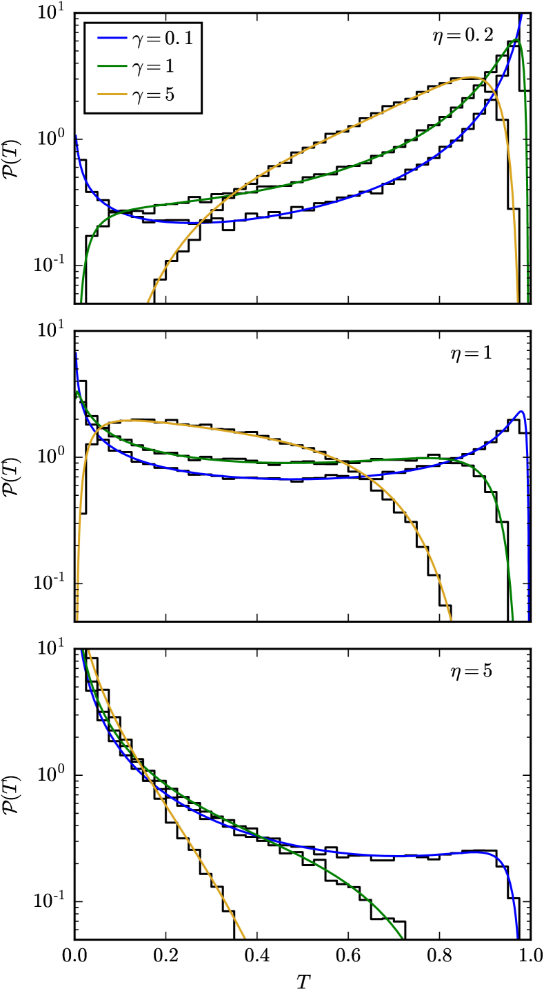
Figure 3: (color online). Transmission distribution for a chaotic background at finite absorption. The curves in color correspond to Eq. (33) and are shown at the absorption rate $\gamma=0.1$ (blue), $\gamma=1$ (green) and $\gamma=5$ (yellow). The coupling to the chaotic background is chosen to be $\eta=0.2$, $1$ and $5$ from top to bottom. Histograms stand for numerical simulations, as detailed in Fig. 2. Notice the disappearance of the bi-modal shape of the distribution at moderate absorption.

The aforementioned bi-modal form of distribution $\mathcal{P}_{0}$ vanishes with increasing absorption. For the weakly coupled background, $\eta\ll 1$, one observes first the diminishing of high transmission peak at $T\sim 1$, and then the eventual depletion of the peak at $T\sim 0$. The situation changes at moderately strong coupling $\eta\gtrsim 1$, when large transmissions become fully suppressed. Figure 3 illustrates such a behaviour, showing also the results of numerical simulations which match the analytical prediction (33) perfectly.

Note that the absorption in the numerical RMT calculations is realized by adding a constant imaginary part to the energy levels of the background. We have also checked the agreement by modelling absorption using fictitious channels as discussed in Brouwer and Beenakker (1997); Savin and Sommers (2003). In this case, one has to rescale the parameters $a$ and $b$ in order to avoid introducing losses on the established channel. The corresponding rescaling is presented in Appendix B.

IV Reflection distributions

The fluctuations in reflection can be studied in a similar way as for the transmission. In the case of vanishing absorption, $\gamma=0$, the reflection distribution can actually be related to Eq. (25). Due to the unitarity of $S$ in this case, we have $|S_{11}|^{2}=1-|S_{12}|^{2}=|S_{22}|^{2}$. Therefore, the distribution of the reflection coefficient $R_{c}=|S_{cc}|^{2}$ ($c=1,2$) is determined by Eq. (25) according to

$$\mathcal{P}_{0}^{\mathrm{(refl)}}(R_{c})=\frac{1}{T_{0}}\mathcal{P}_{0}\left(\frac{1-R_{c}}{T_{0}}\right)$$ (39)

in the region $1-T_{0}\leq R_{c}\leq 1$, being zero otherwise.

In the case of finite absorption, transmission and reflection coefficients are no longer related by flux conservation. The reflection coefficients are readily found from Eqs. (16) and (21) in the explicit form

$$R_{1,2}=\frac{(\eta v\mp r_{0})^{2}+\eta^{2}u^{2}}{(\eta v+1)^{2}+\eta^{2}u^{2}},$$ (40)

where the upper (lower) sign stands for $R_{1}$ ($R_{2}$). One sees that the reflection coefficients are generally different at nonzero $r_{0}$. This is a manifestation of the interference between the equilibrated and direct reflection induced by $S_{0}$ (see the discussion in Sec. II.3).

Following similar steps as leading to Eq. (33), we arrive at the following representation for the distribution of the reflection coefficient $R_{1}$ at $\gamma>0$:

$$\mathcal{P}^{\mathrm{(refl)}}_{\gamma}(R_{1}) =\frac{(1+r_{0})}{2\pi\eta^{2}(1-R_{1})^{2}}\int\limits_{0}^{\infty}\frac{dp\,(1-r_{0}+2\eta w(p))}{\sqrt{p}\,(\hat{w}_{+}+pw_{-})^{2}}$$

$$\phantom{=}\times\frac{(w_{+}+w_{-})}{\sqrt{y(p)}}\mathbb{P}_{0}\left(\frac{1+w(p)^{2}+py(p)}{2w(p)}\right).$$ (41)

Here, we have introduced the following shorthand notations: $\hat{w}_{\pm}=\frac{1}{\eta}\frac{r_{0}\pm\sqrt{R_{1}}}{1\mp\sqrt{R_{1}}}$, $w_{\pm}=\max\{0,\hat{w}_{\pm}\}$, $w(p)={(\hat{w}_{+}+pw_{-})}/{(p+1)}$ and $y(p)=(\hat{w}_{+}-w_{-})[(\hat{w}_{+}-\hat{w}_{-})-p(\hat{w}_{-}-w_{-})]/{(p+1)^{2}}$. The distribution of $R_{2}$ is given by the same formula (41) under the replacement $r_{0}\to-r_{0}$ everywhere there.

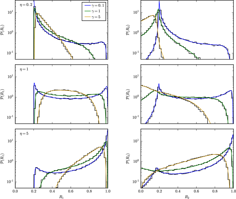
Figure 4: (color online). Distribution of reflection coefficients $R_{1}$ (left panel) and $R_{2}$ (right panel), where $R_{c}=|S_{cc}|^{2}$. The curves in color correspond to Eq. (41) and are shown at the different absorption rates $\gamma=0.1,1$, and $5$ (in blue, green and yellow, respectively) and background coupling $\eta=0.2$, $1$ and $5$ (from top to bottom). The numerical results of RMT simulations are shown as histograms (the same statistics was used as for Fig. 3). The chosen deterministic transmission $T_{0}=0.8$.

Due to the $r_{0}$-dependence of expression (41), it follows that there is a particular difference in the distributions of the two reflection coefficients. Without loss of generality, one can choose $r_{0}<0$ corresponding to the unequal channel couplings, $|b|>|a|$, see Eq. (7). Then we have

$$w_{+}+w_{-}=\left\{\begin{matrix}0,&&R_{1}<r_{0}^{2}\\ \hat{w}_{+},&&R_{1}\geq r_{0}^{2}\end{matrix}\right.$$ (42)

for the reflection coefficient $R_{1}$ and

$$w_{+}+w_{-}=\left\{\begin{matrix}\hat{w}_{+},&&R_{2}<r_{0}^{2}\\ \hat{w}_{+}+\hat{w}_{-},&&R_{2}\geq r_{0}^{2}\end{matrix}\right.$$ (43)

for $R_{2}$. This implies that $\mathcal{P}^{\mathrm{(refl)}}_{\gamma}(R_{1})=0$ identically at $R_{1}\leq r_{0}^{2}=1-T_{0}$, leading to the same gap for small reflections as seen from the case without absorption. The distribution of the other reflection coefficient $R_{2}$ (i.e., in the channel with stronger coupling) does not have such a gap since expression (43) is nonzero for all $R_{2}$.

In Fig. 4 we present a comparison of the analytical result (41) with numerical data, using the same choice of the parameters as for the transmission distribution before. In the general case of finite backscattering, $r_{0}\neq 0$, the reflection distributions in two channels show a distinctly different behavior as discussed above. We have chosen the value of $r_{0}=-\sqrt{0.2}$, corresponding to the established transmission $T_{0}=0.8$. Therefore, the behavior of the reflection coefficient $R_{2}$ changes below $1-T_{0}=0.2$ where the gap in the distribution vanishes. The overall agreement of the theory with numerics is flawless.

V Conclusions and Outlook

In this work, we have formulated an approach to characterise fluctuations in an established transmission that are induced by a chaotic background. Our method is based on the strength function formalism, adopted from and developed in nuclear physics, providing new insights for the applications of the latter in a broader context of wave chaotic systems. The strength of coupling to the background is controlled by the single parameter (1), the ratio of the spreading to escape width. Using RMT to model the chaotic background, we have derived the transmission distribution in an exact form valid at arbitrary uniform absorption in the background. The analytical results are supported by extensive numerics performed by Monte-Carlo simulations with random matrices.

The distribution has a bimodal shape, with two peaks at low and high transmission that are exponentially suppressed at finite absorption. It takes simple limiting forms in the physically interesting cases of weak and strong absorption, which we have discussed in detail as well. Fluctuations in high transmission are found to be affected more strongly by finite absorption, when the background coupling exceeds certain limiting value. These results may be relevant in the reliability context of wireless communication devices Couillet and Debbah (2011).

The method developed is very flexible in incorporating physical properties of the system. In particular, we have neglected absorption of the transmission line itself, however, the latter can be important for experimental realisations, e.g., including ongoing research with chaotic reverberation chambers. Such an extra damping can be naturally accommodated into the theory by a simple rescaling procedure as outlined in Appendix B. Following Rozhkov et al. (2004); Savin et al. (2006), one can also include effects due to nonuniform absorption in the environment. The method can be generalised to other types of the chaotic background (e.g., without time-reversal) as well as to multichannel transmission, where the complete characterisation of both reflection and total transmission in terms of their joint distribution is actually possible and will be reported elsewhere Savin (2017). Therefore, we expect our results to find further applications in studying wave propagation with complex environments.

Appendix A Accuracy of the interpolation formula

In order to ease both implementation and analytical treatment of the exact expressions, one can use a much simpler interpolating formula for function $\mathbb{P}_{0}$, which was suggested in Fyodorov and Savin (2004):

$$\mathbb{P}_{0}^{\mathrm{(int)}}(x)=C_{\gamma}^{-1}\bigl{(}A_{\gamma}\sqrt{\gamma(x+1)}+B_{\gamma}\bigr{)}e^{-\frac{\gamma}{4}(x+1)}.$$ (44)

Here, $A_{\gamma}=(e^{\gamma/2}-1)/2$, $B_{\gamma}=1+\frac{\gamma}{2}-e^{\gamma/2}$, and the normalisation constant $C_{\gamma}=\frac{4}{\gamma}(2\Gamma(\frac{3}{2},\frac{\gamma}{2})A_{\gamma}+e^{-\gamma/2}B_{\gamma})$, with $\Gamma(\nu,\alpha)$ being the upper incomplete gamma function. This formula was earlier found to work surprisingly well when compared to the exact result Savin et al. (2005). Here we show that the level of agreement with the full implementation of the exact $\mathbb{P}_{0}$ yields equally good results.

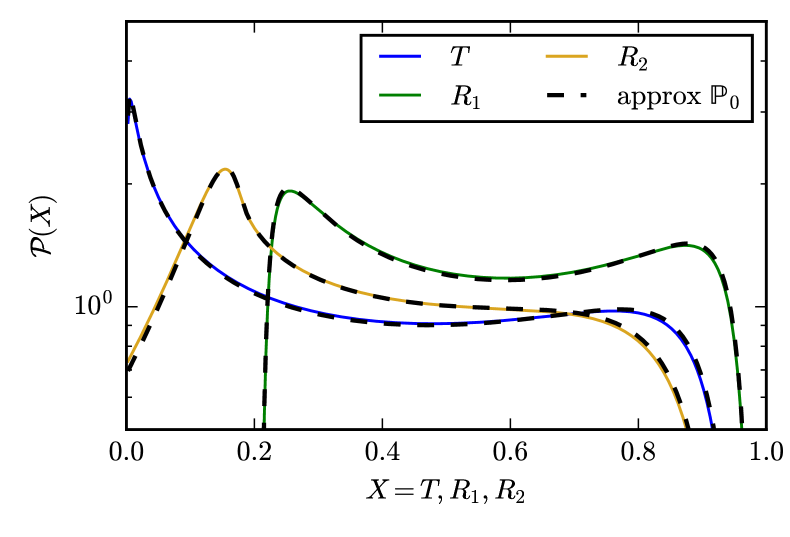
Figure 5: (color online). Accuracy of the interpolation formula. The exact distributions of $T$, $R_{1}$, and $R_{2}$ are shown in solid blue, green, and yellow lines, respectively. Shown in dashed black lines are the same functions from Eqs. (33) and (41) but using the interpolation formula $\mathbb{P}_{0}^{\mathrm{(int)}}$ from Eq. (44). All curves are for $\eta=1$, $\gamma=1$, $T_{0}=0.8$. For other parameter values the correspondence is equally good.

Figure 5 shows two types of the three analytical curves derived from Eqs. (33) and (41): one time calculated using $\mathbb{P}_{0}$ and one time calculated by $\mathbb{P}_{0}^{\mathrm{(int)}}$. The biggest deviations can be found towards $0$ and $1$ or around $r_{0}^{2}$ in the reflection distributions. However, the overall accuracy of the interpolation formula is very good.

Appendix B Absorption of the transmission line

As mentioned in the main text, the derived distributions of transmission and reflection do not include a possible absorption of the single level ${\varepsilon_{0}}$. The latter can be easily incorporated by shifting ${\varepsilon_{0}}\to{\varepsilon_{0}}-(i/2)\Gamma_{\mathrm{abs}}^{(0)}$ in Eqs. (9) and (13), where the absorption width $\Gamma_{\mathrm{abs}}^{(0)}$ of the transmission line is generally different from that of the background. This amounts to replacing ${\Gamma_{0}}\to{\Gamma_{0}}+\Gamma_{\mathrm{abs}}^{(0)}$ and thereby the channel coupling constants $a$ and $b$ by

$$a^{\prime}=a\,\sqrt{1+\Gamma_{\mathrm{abs}}^{(0)}/{\Gamma_{0}}},\quad b^{\prime}=b\,\sqrt{1+\Gamma_{\mathrm{abs}}^{(0)}/{\Gamma_{0}}}.$$ (45)

This results in the following rescaling of the parameters

$$T_{0} \to T^{\prime}_{0}=T_{0}\left(1+\Gamma_{\mathrm{abs}}^{(0)}/{\Gamma_{0}}\right)^{-2}$$ (46)

$$\eta \to\eta^{\prime}=\eta\left(1+\Gamma_{\mathrm{abs}}^{(0)}/{\Gamma_{0}}\right)^{-1}$$ (47)

in the expressions (33) and (41). Using these variables allows us to predict the corresponding distributions also in the case of finite absorption of the transmission line.

References

- Beenakker (1997) C. W. J. Beenakker, “Random-matrix theory of quantum transport,” Rev. Mod. Phys. 69, 731 (1997).
- Alhassid (2000) Y. Alhassid, “The statistical theory of quantum dots,” Rev. Mod. Phys. 72, 895 (2000).
- Mello and Kumar (2004) P. A. Mello and N. Kumar, Quantum Transport in Mesoscopic Systems: Complexity and Statistical Fluctuations. (Oxford University Press, Oxford, 2004).
- Tulino and Verdú (2004) A. M. Tulino and S. Verdú, “Random matrix theory and wireless communications,” Foundations and Trends in Communications and Information Theory 1, 1 (2004).
- Couillet and Debbah (2011) R. Couillet and M. Debbah, Random Matrix Methods for Wireless Communications (Cambridge University Press, Cambridge, 2011).
- Gesbert et al. (2000) D. Gesbert, H. Bolcskei, D. Gore, and A. Paulraj, “Mimo wireless channels: capacity and performance prediction,” in Global Telecommunications Conference, 2000. GLOBECOM ’00. IEEE, Vol. 2 (2000) p. 1083.
- Matthaiou et al. (2010) M. Matthaiou, N. D. Chatzidiamantis, G. K. Karagiannidis, and J. A. Nossek, “On the capacity of generalized- k fading mimo channels,” IEEE Transactions on Signal Processing 58, 5939 (2010).
- Biglieri et al. (2007) E. Biglieri, R. Calderbank, A. Constantinides, A. Goldsmith, A. Paulraj, and H. V. Poor, MIMO Wireless Communications (Cambridge University Press, Cambridge, 2007).
- Bliss and Govindasamy (2013) D. W. Bliss and S. Govindasamy, Adaptive Wireless Communications, MIMO Channels and Networks (Cambridge University Press, Cambridge, 2013).
- Karadimitrakis et al. (2016) A. Karadimitrakis, A. L. Moustakas, H. Hafermann, and A. Mueller, “Optical fiber mimo channel model and its analysis,” in 2016 IEEE International Symposium on Information Theory (ISIT) (2016) pp. 2164–2168.
- Maryenko et al. (2012) D. Maryenko, F. Ospald, K. v. Klitzing, J. H. Smet, J. J. Metzger, R. Fleischmann, T. Geisel, and V. Umansky, “How branching can change the conductance of ballistic semiconductor devices,” Phys. Rev. B 85, 195329 (2012).
- Haake (2001) F. Haake, Quantum Signatures of Chaos. 2nd edition (Springer, Berlin, 2001).
- Mehta (2004) M. L. Mehta, Random Matrices. 3rd Edition (Academic Press, San Diego, 2004).
- Guhr et al. (1998) T. Guhr, A. Müller-Groeling, and H. A. Weidenmüller, “Random matrix theories in Quantum Physics: Common concepts,” Phys. Rep. 299, 189 (1998).
- Stöckmann (2007) H.-J. Stöckmann, Quantum Chaos - An Introduction (University Press, Cambridge, 2007).
- Mahaux and Weidenmüller (1969) C. Mahaux and H. A. Weidenmüller, Shell-Model Approach to Nuclear Reactions (North-Holland, Amsterdam, 1969).
- Verbaarschot et al. (1985) J. J. M. Verbaarschot, H. A. Weidenmüller, and M. R. Zirnbauer, “Grassmann integration in stochastic quantum physics: The case of compound-nucleus scattering,” Phys. Rep. 129, 367 (1985).
- Sokolov and Zelevinsky (1989) V. V. Sokolov and V. G. Zelevinsky, “Dynamics and statistics of unstable quantum states,” Nucl. Phys. A 504, 562 (1989).
- Fyodorov and Sommers (1997) Y. V. Fyodorov and H.-J. Sommers, “Statistics of resonance poles, phase shifts and time delays in quantum chaotic scattering: Random matrix approach for systems with broken time-reversal invariance,” J. Math. Phys. 38, 1918 (1997).
- Mitchell et al. (2010) G. E. Mitchell, A. Richter, and H. A. Weidenmüller, “Random matrices and chaos in nuclear physics: Nuclear reactions,” Rev. Mod. Phys. 82, 2845–2901 (2010).
- Fyodorov and Savin (2011) Y. V. Fyodorov and D. V. Savin, “Resonance scattering of waves in chaotic systems,” in The Oxford Handbook of Random Matrix Theory, edited by G. Akemann, J. Baik, and P. Di Francesco (Oxford University Press, UK, 2011) Chap. 34, pp. 703–722 [arXiv:1003.0702].
- Fyodorov et al. (2005) Y. V. Fyodorov, D. V. Savin, and H.-J. Sommers, “Scattering, reflection and impedance of waves in chaotic and disordered systems with absorption,” J. Phys. A: Math. Gen. 38, 10731 (2005).
- Kumar et al. (2013) S. Kumar, A. Nock, H.-J. Sommers, T. Guhr, B. Dietz, M. Miski-Oglu, A. Richter, and F. Schäfer, “Distribution of scattering matrix elements in quantum chaotic scattering,” Phys. Rev. Lett. 111, 030403 (2013).
- Hemmady et al. (2005) S. Hemmady, X. Zheng, E. Ott, T. M. Antonsen, and S. M. Anlage, “Universal impedance fluctuations in wave chaotic systems,” Phys. Rev. Lett. 94, 014102 (2005).
- Hemmady et al. (2006) S. Hemmady, X. Zheng, J. Hart, T. M. Antonsen, E. Ott, and S. M. Anlage, “Universal properties of two-port scattering, impedance, and admittance matrices of wave-chaotic systems,” Phys. Rev. E 74, 036213 (2006).
- Kuhl et al. (2005a) U. Kuhl, M. Martínez-Mares, R. A. Méndez-Sánchez, and H.-J. Stöckmann, “Direct processes in chaotic microwave cavities in the presence of absorption,” Phys. Rev. Lett. 94, 144101 (2005a).
- Kuhl et al. (2005b) U. Kuhl, H.-J. Stöckmann, and R. Weaver, “Classical wave experiments on chaotic scattering,” J. Phys. A: Math. Gen. 38, 10433 (2005b).
- Dietz et al. (2010) B. Dietz, T. Friedrich, H. L. Harney, M. Miski-Oglu, A. Richter, F. Schäfer, and H. A. Weidenmüller, “Quantum chaotic scattering in microwave resonators,” Phys. Rev. E 81, 036205 (2010).
- Kuhl et al. (2013) U. Kuhl, O. Legrand, and F. Mortessagne, “Microwave experiments using open chaotic cavities in the realm of the effective Hamiltonian formalism,” Fortschritte der Physik 61, 404 (2013).
- Gradoni et al. (2014) G. Gradoni, J.-H. Yeh, B. Xiao, T. M. Antonsen, S. M. Anlage, and E. Ott, “Predicting the statistics of wave transport through chaotic cavities by the random coupling model: A review and recent progress,” Wave Motion 51, 606 (2014).
- Engelbrecht and Weidenmüller (1973) C. A. Engelbrecht and H. A. Weidenmüller, “Hauser-Feshbach theory and Ericson fluctuations in the presence of direct reactions,” Phys. Rev. C 8, 859 (1973).
- Bohr and Mottelson (1969) A. Bohr and B. R. Mottelson, Nuclear Structure (Benjamin, New York, 1969).
- Harney et al. (1986) H. L. Harney, A. Richter, and H. A. Weidenmüller, “Breaking of isospin symmetry in compound-nucleus reactions,” Rev. Mod. Phys. 58, 607 (1986).
- Sokolov and Zelevinsky (1997) V. V. Sokolov and V. Zelevinsky, “Simple mode on a highly excited background: Collective strength and damping in the continuum,” Phys. Rev. C 56, 311 (1997).
- Gu and Weidenmüller (1999) J.-Z. Gu and H.A. Weidenmüller, “Decay out of a superdeformed band,” Nucl. Phys. A 660, 197 (1999).
- Savin and Sommers (2003) D. V. Savin and H.-J. Sommers, “Fluctuations of delay times in chaotic cavities with absorption,” Phys. Rev. E 68, 036211 (2003).
- Sokolov (2010) V. V. Sokolov, “Ballistic electron quantum transport in the presence of a disordered background,” J. Phys. A: Math. Theor. 43, 265102 (2010).
- Zelevinsky and Volya (2016) V. Zelevinsky and A. Volya, “Chaotic features of nuclear structure and dynamics: selected topics,” Phys. Scr. 91, 033006 (2016).
- Sokolov and Zelevinsky (1992) V. V. Sokolov and V. G. Zelevinsky, “Collective dynamics of unstable quantum states,” Ann. Phys. (N.Y.) 216, 323 (1992).
- Fyodorov and Savin (2004) Y. V. Fyodorov and D. V. Savin, “Statistics of impedance, local density of states, and reflection in quantum chaotic systems with absorption,” JETP Lett. 80, 725 (2004).
- Nishioka and Weidenmüller (1985) H. Nishioka and H. A. Weidenmüller, “Compound-nucleus scattering in the presence of direct reactions,” Phys. Lett. B 157, 101 (1985).
- Nock et al. (2014) A. Nock, S. Kumar, H.-J. Sommers, and T. Guhr, “Distributions of off-diagonal scattering matrix elements: Exact results,” Ann. Phys. 342, 103 (2014).
- Savin et al. (2005) D. V. Savin, H.-J. Sommers, and Y. V. Fyodorov, “Universal statistics of the local Green function in quantum chaotic systems with absorption,” JETP Lett. 82, 544 (2005).
- Friedman and Mello (1985) W. A. Friedman and P. A. Mello, “Information theory and statistical nuclear reactions: II. Many-channel case and Hauser-Feshbach formula,” Ann. Phys. (N.Y.) 161, 276 (1985).
- Savin et al. (2001) D. V. Savin, Y. V. Fyodorov, and H.-J. Sommers, “Reducing nonideal to ideal coupling in random matrix description of chaotic scattering: Application to the time-delay problem,” Phys. Rev. E 63, 035202(R) (2001).
- Büttiker (1986) M. Büttiker, “Role of quantum coherence in series resistors,” Phys. Rev. B 33, 3020 (1986).
- Brouwer and Beenakker (1997) P. W. Brouwer and C. W. J. Beenakker, “Voltage-probe and imaginary-potential models for dephasing in a chaotic quantum dot,” Phys. Rev. B 55, 4695 (1997), [Erratum: ibid. 66, 209901(E) (2002)].
- Mello (1995) P. A. Mello, “Theory of random matrices: spectral statistics and scattering problems,” in Mesoscopic Quantum Physics, Proceedings of the Les-Houches Summer School, Session LXI, edited by E. Akkermans, G. Montambaux, J.-L. Pichard, and J. Zinn-Justin (Elsevier, 1995) p. 435.
- not (a) Note that the average . At , implies the uniform distribution for and thus the Cauchy distribution for .
- not (b) We note that although both expressions (37) and (38) are not normalised, they reproduce the exact asymptotic behaviours near the edges. The accuracy of the approximations can be systematically improved by keeping further order terms in (or in ) for weak (or strong) absorption when performing the integration in Eq. (33).
- Rozhkov et al. (2004) I. Rozhkov, Y. V. Fyodorov, and R. L. Weaver, “Variance of transmitted power in multichannel dissipative ergodic structures invariant under time reversal,” Phys. Rev. E 69, 036206 (2004).
- Savin et al. (2006) D. V. Savin, O. Legrand, and F. Mortessagne, “Inhomogeneous losses and complexness of wave functions in chaotic cavities,” Europhys. Lett. 76, 774 (2006).
- Savin (2017) D. V. Savin, to be published (2017).
- (54) “Nemf21: Noisy Electromagnetic Fields – A Technological Platform for Chip-to-Chip Communication in the Century.” See http://www.nemf21.org for detail on the reseach programme and activities.