Machine Vision System for 3D Plant Phenotyping

Abstract

Machine vision for plant phenotyping is an emerging research area for producing high throughput in agriculture and crop science applications. Since 2D based approaches have their inherent limitations, 3D plant analysis is becoming state of the art for current phenotyping technologies. We present an automated system for analyzing plant growth in indoor conditions. A gantry robot system is used to perform scanning tasks in an automated manner throughout the lifetime of the plant. A 3D laser scanner mounted as the robot’s payload captures the surface point cloud data of the plant from multiple views. The plant is monitored from the vegetative to reproductive stages in light/dark cycles inside a controllable growth chamber. An efficient 3D reconstruction algorithm is used, by which multiple scans are aligned together to obtain a 3D mesh of the plant, followed by surface area and volume computations. The whole system, including the programmable growth chamber, robot, scanner, data transfer and analysis is fully automated in such a way that a naive user can, in theory, start the system with a mouse click and get back the growth analysis results at the end of the lifetime of the plant with no intermediate intervention. As evidence of its functionality, we show and analyze quantitative results of the rhythmic growth patterns of the dicot Arabidopsis thaliana(L.), and the monocot barley (Hordeum vulgare L.) plants under their diurnal light/dark cycles.

1 Introduction

Autonomous and accurate real time plant phenotyping is a quintessential part of modern crop monitoring and agricultural technologies. Non-invasive analysis of plants is highly desirable in plant science research because traditional techniques usually require the destruction of the plant, thus prohibiting the analysis of the growth of the plant over its life-cycle. Machine vision systems allow us to monitor, analyze and produce high throughput in an autonomous manner without any manual intervention. Among several parameters of plant phenotyping, growth analysis is very important for biological inference. Functional analysis of growth curve can reveal many underlying functionalities of the plant [1]. A plant’s growth pattern can reveal different biological properties in different environmental conditions. For example, leaf elevation angle has impact from the amount of sunlight [2]. In direct sunlight, leaves exhibit more elongation than when the plant is shaded. Similar kinds of behaviour are exhibited for rosette size, stem height, plant surface area and volume. Imaging techniques are very effective in terms of non-invasive and accurate analysis. While 2D imaging techniques have been used extensively in the literature, it has some inherent limitations. The advantage of 3D over 2D are numerous. For example, consider the area of a leaf. If the leaf is curved, the 3D area will be significantly different from the area computed from it’s 2D image. Another restriction of 2D is that it is often difficult to measure 3D quantities such as the surface area or the volume of a plant without doing error prone and potentially complex calculations, such as a stereo disparity calculation from stereo images, to get the 3D depth information that is a precursor to these calculations. Recently, 3D laser scanners are being used in many applications for studying plant phenotyping. As far as we know, we are the first to capture the full 3D structure of a plant as a single closed 3D triangular mesh using a (near-infrared) laser scanner.

With the advancement of robotic technologies, automation tasks have become easier. Apart from automating the phenotyping process, the data collection can also be automated efficiently in real time. However, there are a number of challenges involved in accomplishing this, such as communication among the hardware devices, reliable data transfer and analysis, fault tolerance, etc. We have developed a 3D plant phenotyping vision system which is capable of monitoring and analyzing a plant’s growth over it’s entire life-cycle. Our system has several parts. First, a gantry robot system is used for the automation of data collection process. The robot is programmable and can be moved around the plant by specifying a particular trajectory. A 3D laser scanner is the robot arm’s payload. The scanner can record 3D point cloud data from a number of viewpoints about the plant. The robot moves from one viewpoint to another, and communicates with the scanner to take a scan of the plant under observation. In the current setup, the plant is scanned six times a day from $12$ viewpoints at $30^{\circ}$ increments about $360^{\circ}$ (we obtain six 3D triangular meshes a day). The 12 viewpoints result in overlapping range data between adjacent views, allowing the merging of all the views into a single 3D triangular mesh representing the whole plant. Note that our laser scanner uses a near infrared beam (about $825nm$) and can scan the plant in the light and in the dark equally well.

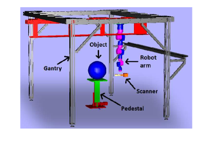
Figure 1: Schematic diagram of the gantry robot system

In this paper, we report growth results and analysis for 3 weeks of the life-cycle of wild type Arabidopsis thaliana(L.) and barley plants. We also attempted to measure the growth of a conifer plant, but we could not capture the individual needle data at a sufficiently high enough resolution to allow good range view merging (see Section 7 for a complete description of this experiment). We have grown all our plants in the indoor growth chamber with proper environmental conditions (e.g. light, temperature, wind, humidity, etc.). The reason for using the Arabidopsis plant is that, this plant has used extensively as a model plant in biology and was the first plant whose genome was completely sequenced [3]. In later experiments (not yet designed or performed) we will investigate the effect of generic modifications on the plant’s growth rate as compared to the wild type.

Reconstructing a plant’s 3D model from multiple views is extremely challenging [4, 5, 6, 7]. Unlike using a rigid model like the Stanford bunny, reconstructing a highly non-rigid thin plant is difficult. We use a new multi-view alignment (registration) algorithm on individual 3D point clouds obtained by our scanning to obtain a 3D triangular mesh of the growing plant. Given this mesh, we can compute the 3D surface area and volume of the plant. We propose that area and volume make good plant growth metrics.

We have extended the basic system as reported in a conference paper [8] in several ways. We now provide a more detailed analyses and infer biologically relevant results for plant growth measurements. More specifically, we present the following new contributions in this paper. First, we have made the system work throughout the lifetime of the plants in a fully automated way, which is challenging due to the complex nature of the whole system. Second, we propose feature point matching of two views of a plant for rough initial registration without knowing sensor/camera location or rotation angles. Our previous work has assumed we had rough a priori knowledge about how much the sensor was rotated for each view [8], now the angle between adjacent views can be arbitrary, although they still have to overlap for the merging to work. Third, we build 3D models of the plants, and compute surface area and volume of the reconstructed meshes by using an efficient triangulation algorithm. Fourth, we analyze the growth curves of the plants and demonstrate the accuracy of the system to capture the well known diurnal growth pattern of plants.

In the next section we discuss the related literature. Then the system components are explained in detail, followed by their integration into a complete system and finally the operation of that system. Subsequently the multi-view reconstruction algorithm is discussed and we show experimental results and derive conclusions based on those results.

2 Related Work

In last decade there has been tremendous progress in automated plant phenotyping and plant imaging technologies [9]. Accurate phenotyping of plants is crucial in analyzing different properties of plants in different environmental conditions. Traditionally biologists have used naïve (manual) methods for plant phenotyping. This led to low throughput and sometimes questionable accuracy. Accuracy and throughput are major factors in mass scale analysis. To build a real time plant phenotyping system with high accuracy, the system needs to be fully automated. A truly automated system should allow a naïve user to operate the phenotyping process and obtain the growth analysis as a ready-made end product. As many of the current phenotyping technologies focus on software development for processing the data [10, 11], automated collection of data is also becoming state of the art [12, 13] over tedious manual techniques [14] . However, most of the automated systems have their limitations. Either they are dependent on particular types of plant(s), or on their size and geometrical structures. In an attempt to generalize the phenotyping process, computer vision based system design is becoming very useful in studying plant growth, and a body of work has been reported in that area [15, 16, 17].

Among several components of phenotyping, growth analysis is extremely important [18]. A plant’s growth is highly affected by the environmental conditions. Accurate measurement of a plant’s growth can reveal much information which can be useful for accelerating crop production. In recent years, different aspects of plant phenotyping and growth measurement have appeared in the literature.

Detection and tracking of plant organs (e.g. flowers, buds, stems, leaves, fruit) have gained the interest of many researchers. A machine vision system for fruit harvesting was proposed by Jimenez et al. [19]. They used an infrared laser scanner to collect data and used computer vision algorithms to detect fruit on a plant using their colour and morphological properties. This type of automated system is in great demand for fruit harvesting and agricultural engineering. Automated classification of plant organs can be useful for tracking a specific area of the plant over time. Paulus et al. [20, 21] showed a feature based histogram analysis method to classify different organs in wheat, grapevine and barley plants. A segmentation algorithm to monitor grapevine growth was presented by Klodt et al. [22]. A similar type of work on plant organ segmentation by unsupervised clustering was proposed by Wahabzada et al. [23]. Paproki et al. [24] showed a 3D approach to measure plant growth in the vegetative stage. Multiple images of a plant are taken from different viewpoints and the plant mesh is generated via multi-view reconstruction. Then different organs of the plant mesh are segmented and parameterized. The accuracy of the parameterization is validated by comparison with manual results. Golbach et al. [25] used a multi-camera set-up and a plant’s 3D model is reconstructed via projection matrices. They demonstrated automatic segmentation of leaves and stems to compute geometric properties such as area, length, etc. and validated the result by comparing with ground truth data destructively by hand.

Other recent work focused on detecting specific patterns in a plant’s leaves to determine the particular condition of the plant. Analysis is performed by tracking leaves and detecting colour properties of the leaves. However, segmentation of plant leaves in different imaging conditions is a challenging task [26]. Alenyà et al. [27] performed a robotic experiment for automated plant monitoring. A camera mounted to the robot arm takes images of the plant and the leaves are segmented. Then the robot arm moves to the desired location to track a particular leaf. Dellen et al. [1] performed a $12.5$ days experiment to analyze leaf growth of tobacco plants. They segmented the leaves by extracting their contours and fitted second order polynomial to model each leaf. A graph based algorithm is used to perform tracking of leaves over time. Kelly et al. [28] showed an active contour based model to detect lesions in Zea mays. This crop is widely used and detecting the lesions can be helpful to detect disease in the early growth stage. Xu et al. [29] presented an approach to detect nitrogen and potassium deficient tomatoes from the colour images of the leaves. Recent work on tracking leaves of rosette plants can be found in [30].This work can be useful for measuring growth rate of a particular leaf.

Building a 3D plant model from multi-views is a challenging task. The complex geometry of plants make the problem of 3D surface reconstruction difficult. Pound et al. [31, 32] proposed a level set based approach to reconstruct the 3D model of a plant from multiple views. Their reported results are promising in that they show that their 3D model closely mimics the original plant structure. Santos et al. [33] showed a feature matching based approach to build the 3D model of a plant using a structure from motion (SfM) algorithm. Multiple images of the plant are taken manually and camera positions are recovered to build a 3D model of the plant. However, the method is highly dependent on local features. This type of idea exploiting SfM to generate a 3D model of a plant is used in [34] to compute plant height and leaf length accurately.

Rhythmic patterns of a plant’s growth are well studied in the biological literature [35, 36, 37]. A system capable of detecting diurnal growth patterns can be reliably used to monitor the growth pattern of different species in different conditions. Imaging based techniques are becoming more popular in such analysis [38]. A vision based system to study the circadian rhythm of plants was presented by Navarro et al. [39]. The automated system captures the diurnal growth pattern using 2D imaging techniques. A laser scanning based 3D approach was reported by Dornbusch et al. [2], which shows the diurnal pattern of leaf angle in different lighting conditions. Tracking and growth analysis of a seedling by imaging technique was studied by Benoit et al. [40]. Barron and Liptay et al. [41, 42] used a front and side view of a young corn seedling imaged by a near-infrared camera to obtain growth for 1-3 days. The growth was shown to be well correlated by root temperature (Pearson coefficient 0.94).

Godin and Ferraro [43] presented a structural analysis of tree structures which can be useful in plant growth analysis. Augustin et al. [44] modelled a mature Arabidopsis plant for phenotype analysis. They demonstrated extraction of accurate geometric structures of the plant from 2D images which can be useful for phenotyping studies of different parts of the plant. Li et al. [45] performed a 4D analysis to robustly segment plant parts to localize buddings and bifurcations accurately using a backward-forward analysis technique.

Most of the methods discussed above have several limitations. None of these systems are designed to monitor a plant’s growth for it’s whole lifetime in an automated manner using 3D imaging technique. To the best of our knowledge, we are the first to report a fully automated system which operates in near real time over the lifetime of a plant using laser scanning technology. We present a novel approach to study plant growth in truly automated manner using 3D imaging technique. The system is described in next section.

3 System Description

The proposed system has several parts which are integrated to make a fully autonomous system. Each component is explained separately below.

3.1 Gantry Robot

A schematic diagram of the robotic system (manufactured by Schunk Inc., Germany) is shown in Figure 1 comprising an adjustable pedestal and a 2-axis overhead gantry carrying a 7-DOF robotic arm. The plant is placed on the pedestal which can be moved up and down to accommodative different applications and plant sizes.

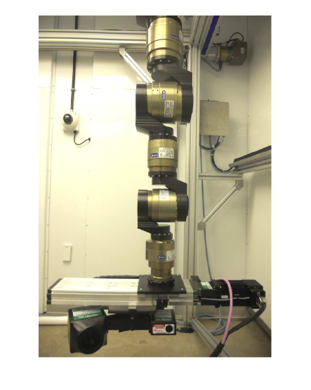
Figure 2: Robot arm

The 7-DOF robotic arm in Figure 2 provides a high level of flexibility for controlling the position and orientation of the 3D scan head, while the 2-axis gantry provides an extended workspace. The specification details of the robot is shown in Table I. We can see that the accuracy and repeatability are both 0.1 $\mu$m.

TABLE I: Robot Specifications

Degrees of freedom		$7$
Dimensions	x	$3m$
	y	$2m$
	z	$1.8m$
Accuracy		$0.1\mu m$
Repeatability		$0.1\mu m$
Speed		$1$m/s
Payload		$10$ kg

We have programmed the robot to move in a circular trajectory around the plant to take scans. Initially the robot stays in it’s home position with the arm resting vertically downwards (Figure 3). After the initiation of the commands, it moves from home position to the desired location by alternating macro and micro joint movements.

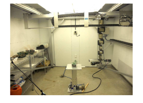
Figure 3: Robot room where the experiment was performed

We maintained a horizontal distance of $0.56m$ from the center of the pedestal to the vertical axis of the robot arm, and $0.26m$ from the pedestal plane to the scanner. These distances were set empirically to obtain the best scan data.

3.2 Scanner

We use a SG1002 ShapeGrabber range scanner, which is the payload of the robot arm. This scanner can measure dense depth maps of the visible surface of an object in point cloud format. We also store intensity value of each point in the cloud, although we do not currently use these values. The scanner uses near-infrared light at $825$nm (versus visible red light at $660$nm for most scanners) which is thought (by Grodzinski and Hüner, two co-authors on this paper) to have minimal effects on plant growth (currently undocumented). Different parameters of the scanner (e.g. Field of View, laser power, etc.) are set empirically. We have performed the whole experiment with laser power $1.0$mW (means the laser has a beam radius of $1.0$mm). It takes about $1$ minute for a single scan to produce point cloud data having resolution of $0.25mm$ spacing between two points. The scanner software Communicates over a UDP (User Datagram Protocol) link with the robot control software. Each time, after the robot stops at a scanning position, it communicates with the scanner to take a scan and then moves to the next position.

3.3 Growth Chamber

We have designed the whole robotic set-up inside a growth chamber (manufactured by BioChambers Inc., Canada). The chamber is fully programmable allowing control of the temperature, the humidity, the fan speed and light intensity. Also, it can be monitored remotely using a camera. The chamber is $5.2m^{2}$ and is equipped with a combination of $1220$mm T5HO fluorescent lamps and halogen lamps The whole chamber is a dedicated embedded system, and can be controlled from the robot control software,

4 Alignment of multi-view scans

Multi-view alignment is a major task in building a 3D model of an object. Pairwise registration is a crucial part in performing multi-data alignment and this has been studied extensively in the computer vision literature [46, 47, 48, 49]. However, registration of thin non-rigid plant structure is very challenging and little studied. Although Iterative Closest Point (ICP) [50] and it’s variants [51, 52, 53] have been successful in some cases, registering highly non-rigid thin plant structures is still problematic.

Recently, the use of Gaussian Mixture Models (GMM) have been popular in registering two non-rigid point sets [54]. The key idea is to represent discrete points by continuous probability density functions so that the problem of minimizing discrete optimization problem can be reduced to a continuous optimization problem.

Mathematically, a Gaussian mixture model can be stated as the weighted sum of M component Gaussian densities:

$$p(\mathbf{x}|\lambda)=\sum_{i=1}^{M}w_{i}\ g(\mathbf{x}|\mathbf{\mu}_{i},\mathbf{\Sigma}_{i}),$$ (1)

where $\mathbf{x}$ is a $d$-dimensional vector, $w_{i}(i=1,...,M$) are weights of each mixture $g$ having mean $\mathbf{\mu}_{i}$ and covariance $\Sigma_{i}$, and $\lambda=\{w_{i},\mathbf{\mu}_{i},\mathbf{\Sigma}_{i}\}$ are the parameters. The registration problem can be formulated as the minimization of the discrepancy between two Gaussian mixtures by minimizing the following cost function [54]:

$$d_{L_{2}}(\mathcal{S},\mathcal{M},\Theta)=\int(gmm(\mathcal{S})-gmm(\mathcal{T}(\mathcal{M},\Theta)))^{2}\>\mathrm{d}x$$ (2)

where $\mathcal{M}$ is the model point set and $\mathcal{S}$ is the scene (data) point set. The function $gmm(\mathcal{P})$ denotes the Gaussian mixture density constructed from $\mathcal{P}$. The aim is to find parameters $\Theta$ which minimizes the above cost function using $L_{2}$ norm as the distance measure. Myronenko et al. presented a Coherent Point Drift (CPD) algorithm [55] where the center of Gaussians are moved together for registering two point sets. The method is state of the art and has been applied to many applications. These methods work reasonably well for pairwise registration but aligning multi-data using them is problematic.

We use an extension of CPD for aligning multi-datasets, proposed by Brophy et al. [5]. Given two point clouds, $\mathbf{X}=(\mathbf{x}_{1},\mathbf{x}_{2},...,\mathbf{x}_{m})^{T}$ and $\mathbf{Y}=(\mathbf{y}_{1},\mathbf{y}_{2},...,\mathbf{y}_{n})^{T}$, in general for a point $\mathbf{x}$, the GMM probability density function will be:

$$p(\mathbf{x})=\sum_{i=1}^{M+1}P(i)p(\mathbf{x}|i),$$ (3)

where

$$p(\mathbf{x}|i)=\frac{1}{(2\pi\sigma^{2})^{d/2}}\ exp[-\frac{||\mathbf{x}-\mathbf{y}_{i}||^{2}}{2\sigma^{2}}].$$ (4)

Instead of maximizing the GMM posterior probability, the negative log-likelihood function can be minimized to obtain the optimal alignment:

$$E(\theta,\sigma^{2})=-\sum_{j=1}^{N}log\sum_{i=1}^{M+1}P(i)p(\mathbf{x}_{j}|i),$$ (5)

where

$$P(i|\mathbf{x}_{j})=P(i)p(\mathbf{x}_{j}|i)/p(\mathbf{x}_{j}).$$ (6)

Then the Expectation Maximization algorithm is used iteratively to optimize the cost function.

Inspired by the work in rigid registration by Toldo et al. [56], an “average” scan is constructed, to which we register all other scans. For a scan $X$, we find the set of points that are the Mutual Nearest Neighbours (MNN) to a point in the scan, and then we calculate a scan that is composed of the calculated centroids from each point. Once the initial registration is complete, we use CPD in conjunction with MNN to recover the non-rigid deformation field that the plant undergoes between the capture of each scan. At this point, the scans should be approximately aligned to one another. We then construct the centroid/average scan and then register to it.

Basically, the method is a two step process, beginning with aligning the scans approximately. We then register a single scan to the “average” shape, constructed from all other scans, and update the set to include the newly registered result. We perform the same process with all other sets of scans. In this way, we avoid accumulation of merging error. In general, CPD alone is effective in registering pairs with a fair amount of overlap, but when registering multiple scans, our method achieves a much better fit than CPD by itself, utilizing sequential pairwise registration.

4.1 Rough Initial Alignment

Although the multiple view registration algorithm works well in aligning different scan data, registering two views with huge rotation angle difference can pose difficulties. Unfortunately, after decades of research on point cloud registration, state of the art algorithms fail when the views are not roughly aligned. The problem is more challenging for the cases of complex plant structures due to occlusion and local deformation between two views [6, 7, 57]. Note that the rough initial alignment alone is not sufficient to register two views, and this is a pre-processing step of the actual registration algorithm as discussed in the previous section.

One approach to estimate the rough alignment of two views is to find corresponding feature points. However, because of the complex structure of the plants, finding repeatable features is extremely hard [1] and typical feature point matching algorithms fail. Junctions are strong features for plant-like structures. We adopt the idea of using junction point of branches as feature points and then match these features [57]. However, the idea in [57] for detecting junction points does not consider occlusion in leaves. This results in false feature point detection, which may not be repeatable in two views. We extend our algorithm [57] using a simple but effective density clustering technique as discussed below. Lin et al. have proposed a similar idea [58].

4.1.1 Feature Clustering

The basic idea of our junction detection algorithm [57] is to first extract local neighbourhood around every point using kd-trees and perform a statistical dip test to determine the non-linearity in the data. Then the branches are approximated by fitting straight lines to the point cloud. Finally straight line equations are solved to determine if they intersect in the local neighborhood. This approach results in detection of multiple feature points around the junction, because all the points around a small neighbourhood at the junction are potential candidates of true junction points, from which the best candidate is picked up by non-maximal suppression of the dip value. But this idea also detects false feature points as junctions in occluded leafy areas. We handle this problem by applying density based clustering to extract the true junctions and filter out the rest of the feature points [59].

The idea of density based clustering is to find groups of points that are denser than the remaining points. As true junction features tend to appear with higher density than false junctions, we cluster the detected feature points to find the cluster of points that are formed at true junction points. We use the density based clustering algorithm proposed by Ester et al. [59]. The algorithm does not need the number of clusters to be known in advance (unlike k-means) and can perform clustering in the presence of large number of outliers. Finally, we compute the centroid of each cluster to find the true junctions and match these features using our subgraph matching technique [57]. Figure 4 illustrates this idea. It shows a single view of a plant having occlusions. Red dots represents feature points detected by our junction detection algorithm [57]. The clustering algorithm detects clusters around true junction points (denoted by blue circles) and discards the remainder of the points as outliers.

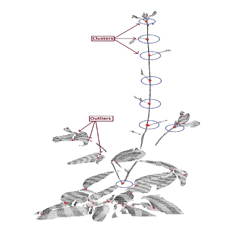
Figure 4: Demonstration of feature clustering. Red dots represent junction feature points [57]. Density clustering algorithm [59] detects clusters at true junctions (denoted by blue circle) and treats false feature points as outliers.

5 System Integration

We integrate the chamber, robot and scanner. The system components and their connections are shown in Figure 5. The robot and scanner are operated from different computers which communicate over a dedicated UDP link. The chamber is accessed remotely over the internet.

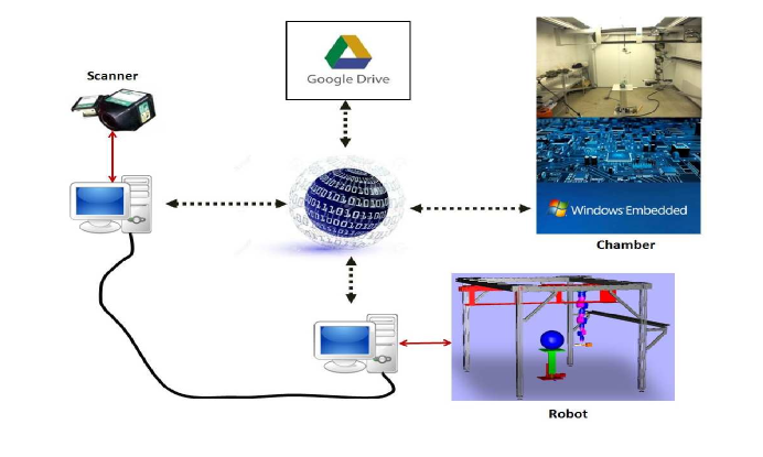
Figure 5: High level view of the system

Communication between the chamber and robot operation needs to be done frequently. While scanning a plant, we need to shut down or significantly decrease the fan speed inside the chamber (at present we just shut it down completely), otherwise the scan data will be erroneous as the plant will be jittering (this makes the multiple view reconstruction problem extremely difficult). Also, experimenting in different lighting conditions (short day versus long day) needs communication between the chamber and the scanning schedule of the robot. Before starting the experiment, chamber parameters are set according to the need of the application. During the experiment before a set of scans, the robot communicates with the chamber, turns off the fan (and light if needed), and restores the default chamber settings when the scan is completed. This process is repeated at each scan.

As the size or dimension of the plant is not known in advance, determining the scanning boundaries to enclose the whole plant needs to be done dynamically during each scan. Moreover, as the plant grows, it may lean towards a particular direction, which requires the scanner position to be adjusted accordingly. We perform a simple bounding box calculation before performing each scan (Figure 6). Before doing the actual scanning, a pre-scan procedure is performed from 2 directions (front and side as shown in the figure). From these scans, the centre of the bounding box of the plant is approximated and used to update the centre of rotation for the circular scanning trajectory. Once the plant centre has been determined, the system causes the gantry and robotic arm to translate and rotate the scan head to specified discrete positions around the plant.

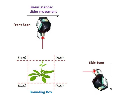
Figure 6: Computing the bounding box to determine the center of the plant

At each scanning position, the system waits 10 seconds to allow the plant and the scanner to settle before initiating a scan. Once a scan has finished, the resulting scan data are analyzed to ensure that the plant has been fully captured (i.e. there is no clipping via a bounding box calculation). Sometimes the scanner FOV is not wide enough to capture the full width of the plant due to a limited travel of the scanner’s linear stage ($0.2m$). In that case, an extra scan of that view is automatically made by sliding the scanner in a sideways direction. From empirical observations, for plants like Arabidopsis, no more than 3 partial scans are needed to enclose a single view as illustrated in Figure 7. Usually, if the plant is not too wide, a single view from $P$ is sufficient. Otherwise, we perform side scans at positions $P_{1}$, $P_{2}$ and $P_{3}$. We want to emphasize that all scanning, including this side scanning is fully automated in our system. Currently, we have not allowed for upwards scanning, where the plant could grow out of range by growing too high (this has never happened in all our scanning experience).

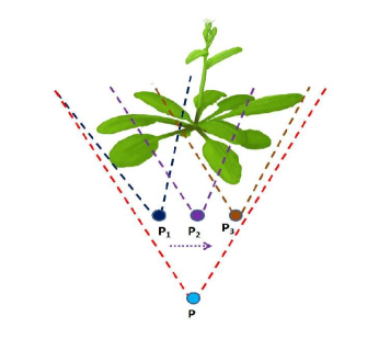
Figure 7: Scanner Field of View (FOV) to enclose the whole plant. When the plant is big, one scan can’t capture the whole plant and multiple scans are required. This is done automatically.

We operate the whole system from a single GUI. Once the system is started, theoretically, it can continue scanning and processing until the experiment is terminated. We say “theoretically” here as some unexpected events, such as network failure, can occur. Network failure requires human intervention to fix.

6 Experimental Results

First we have performed a 21 day experiment with a wild type Arabidopsis plant (after which the plant was falling down) with a $12/12$ hours light/dark cycle at the temperature of $25^{\circ}$C and a light intensity of $250\mu mol$ photons $m^{-2}s^{-1}$. We also performed another 15 day experiment with barley under the same conditions. Although the algorithms used in the different stages are not new, the main challenge was to make the whole system work continuously for the life-cycle of the plant. We encountered several problems while integrating the system parts (robot, chamber, scanner, etc). As the robot and the chamber needed to communicate frequently (every $4$ hours as we are performing $6$ scans per day, throughout the life of the plant), there were issues of lost communication due to network failure and infrequent hardware faults (e.g. problems in electronic chips at robot joints, etc).

6.1 Merging of multi-view plant point cloud

Using the reconstruction algorithm discussed above, we performed alignment of the multi-view point cloud data of the growing plant over time. We used Sharcnet computing machines for simultaneous processing of large amount of data while the scan data was collected throughout the life of the plant. The merged point cloud data for fully grown Arabidopsis plant (day $20$^th) and the barley plant (day $15$^th) are shown in Figures 8 and 9 respectively. Each colour represents different scans.

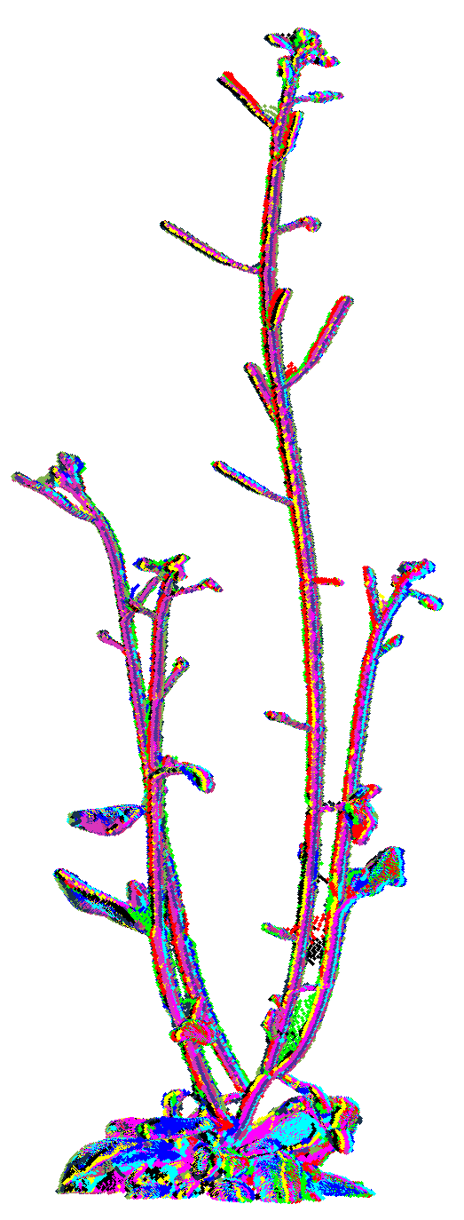
Figure 8: Reconstructed Arabidopsis plant point cloud (different colors indicate different scans)

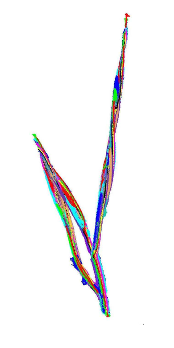
Figure 9: Reconstructed Barley plant point cloud (different colors indicate different scans)

6.2 Polygonal mesh formation

Once we have the aligned point cloud from the multi-view data, it needs to be triangulated in order to compute the mesh surface area and volume. Accurate triangulation of point cloud data is a challenging problem. An efficient triangulation should represent all the details of the shape of the object. Triangulation of plant structures is more challenging due to the thin branches. Although Delaunay triangulation is typically used for modeling a surface, the algorithm does not produce good result for plant structures. We used the $\alpha$-shape algorithm [60] for triangulation. The algorithm works well when its parameters are properly tuned .

6.3 $\alpha$-Shape Triangulation

Let $P=\{p_{1},\cdots,p_{n}\}\subset\mathbb{R}^{d}$ be a set of points, which are called sites. A Voronoi diagram is a decomposition of $\mathbb{R}^{d}$ into convex polyhedra. Each region or Voronoi cell $\mathcal{V}(p_{i})$ for $p_{i}$ is defined to be the set of points $x$ that are closer to $p_{i}$ than to any other site. Mathematically,

$$\mathcal{V}(p_{i})=\{x\in\mathbb{R}^{d}~{}~{}|~{}~{}||p_{i}-x||\leq||p_{j}-x||~{}\forall j\neq i\},$$

where $||.||$ denotes the Euclidean distance. The Delaunay triangulation of P is defined as the dual of the Voronoi diagram.

The $\alpha$ complex of $P$ is defined as the Delaunay triangulation of $P$ having an empty circumscribing sphere with squared radius equal to or smaller than $\alpha$. The $\alpha$ shape is the domain covered by alpha complex. If $\alpha=0$, the $\alpha$-shape is the point set $P$, and for $0\leq\alpha\leq\infty$, the boundary $\partial\mathcal{P}_{\alpha}$ of the $\alpha$-shape is a subset of the Delaunay triangulation of $P$. The main idea of the algorithm is that the space generated by any point pairs can be touched by an empty disc of radius $\alpha$. The value of $\alpha$ controls the level of detail in triangulation. The algorithm is simple and effective. We have empirically chosen $\alpha=0.6$ for the plants. Also note that we have already performed “smoothing” of the point cloud while applying Gaussians, so we do not need further surface smoothing (such as Poisson smoothing). Example results are shown in Figures 10 and 11. The rectangular cutouts show some smaller portions of the plants at higher resolution. The surface area is simply the summation of area of each triangle in the mesh and volume can be computed using the technique described by Zhang et al. [61]. The “loop” structure is due to the angle by which the barley plant is viewed, some of parts of the plant occludes other parts.

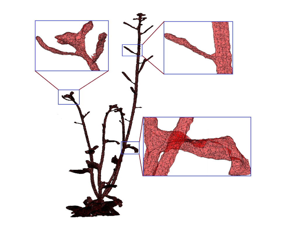
Figure 10: Triangulated Arabidopsis plant data

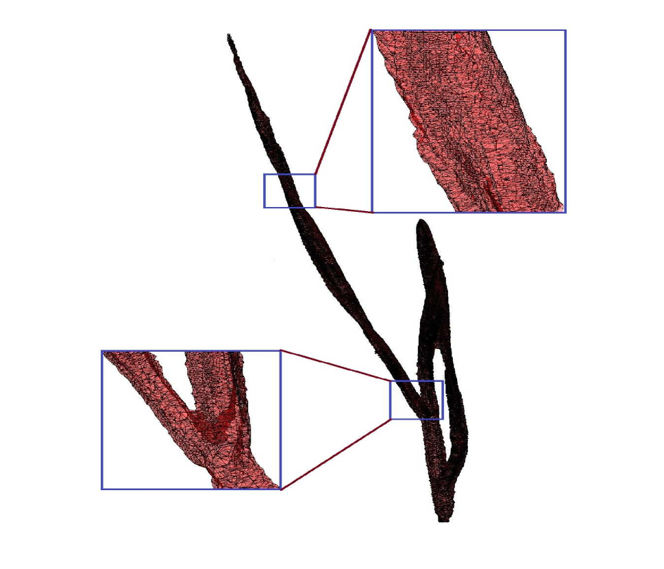
Figure 11: Triangulated Barley plant data

6.4 Biological Relevance

The fact that plants grow mostly at night and shrink in the day time is well known [62]. It is observed that the changes in stem diameter depends on the lighting conditions [35, 36, 37]. While the diurnal nature of plant growth can involve changes in stem length, width, diameter, leaf surface area, we have observed the diurnal pattern in both volume and surface area of the plant. The mesh surface area and volume are plotted against time in the same graph for Arabidopsis plant in Figure 12. A similar plot for barley plant is shown in Figure 13. In the graphs, red dots represent night time scans and blue dots represent day time scans. As we have $6$ scans per day, there are $3$ blue dots followed by $3$ red dots in the graph. For the Arabidopsis experiment we had $4$ scans missing due to networking problems. These missing data are generated by taking the average of previous and next scan data. These are shown as green dots in Figures 12 and 13.

It can be noticed from the growth curves that the plants exhibited more growth in the night time than in the day time, which supports the biological relevance of diurnal growth pattern of plants. Finally, note that the changes of volume are greater than the changes of surface area in the later period of the growth cycle (this is logical as volume grows faster that area).

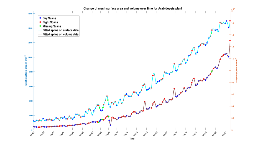
Figure 12: Diurnal growth pattern of mesh surface area and volume for the Arabidopsis plant. The red dots represent night time scans, the blue dots represent day time scans and the four green dots represent missing scan data. A spline is fitted to both surface and volume scan data (shown in different colours). The $y$-axis in the left and right hand side represents the range of surface area and volume data respectively.

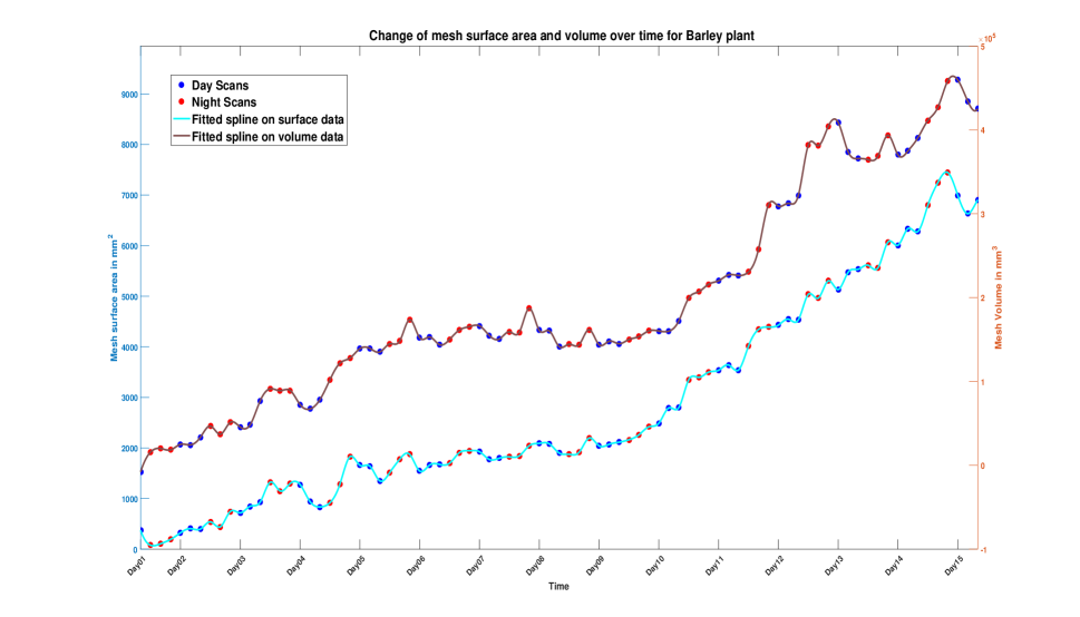
Figure 13: Diurnal growth pattern of mesh surface area and volume for the barley plant. The red dots represent night time scans while the blue dots represent day time scan data. A spline is fitted to both surface and volume scan data (shown in different colours). The $y$-axis in the left and right hand side represents the range of surface area and volume data respectively.

The initial short stage of plant growth looks linear, the long intermediate stage of plant growth looks exponential while the short end stage of plant growth looks stationary (or constant). Often, biologists compute the growth rate as the logarithm of mesh surface area values and then fit a straight line to this data, yielding the maximum exponential growth rate. Figures 14a and 14b show the surface area and volume growth rates for the Arabidopsis plant while Figures 14c and 14d show the surface area and volume growth rates for the barley plant. The growth rates (slopes of the growth rate lines) are printed as text items in the upper left corner of each graph and show that the surface area and volume growth rates for the two plants are roughly the same. However, as the growth rate of Barley plant exhibits a highly non-linear pattern, fitting a straight line to compute the actual growth rate may not be appropriate. We believe instead that a polynomial curve fitting scheme might be a better, with local growth rates being the slopes of the tangents on this curve.

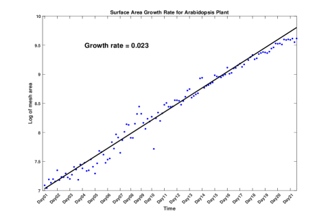
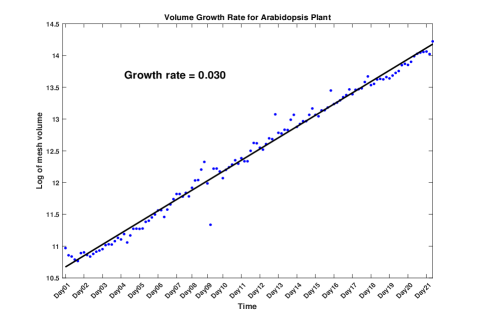
(a)	(b)
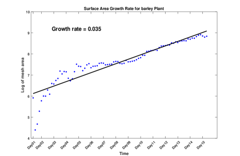
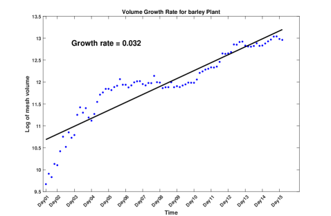
(c)	(d)

Figure 14: (a) and (c): the surface growth rate lines and (c) and (d): the volume growth rate lines for the Arabidopsis and barley plants.

7 Limitations of the System and Future Work

We have presented a fully automated system capable of analyzing plant growth throughout the lifetime of the plant. We have validated the accuracy of the system by experimenting with two real plants throughout their lifetime, which clearly shows the diurnal nature of plant growth. This type of system can be used for comparing growth patterns of different types, varieties and species in different environmental conditions in autonomous way. The robot can also be used to perform tracking of different plant organs over time. We believe that the proposed system is general enough to perform various biological relevant experiments in a non-invasive and automatic manner.

One minor limitation of the system is that, it can process one plant at a time, but this can easily be changed for future scanning. To increase plant throughput, we can scan multiple plants at a time. We have also begun to study more challenging plants like the conifer. Accurate reconstruction of the conifer is challenging due to the fine structures of its needles. For example, Figure 15 shows the reconstruction of 12 view of a conifer tree with a single cutout shows one part of its surface at higher resolution. We can see that the range data does not capture the needle structure adequately. Ideally, each needle of the conifer should be clearly and completely visible in the reconstructed point cloud but this is not the case. The initial growth pattern of conifer plant is shown in Figure 16. The growth rate calculated from this pattern is a flat horizontal line (not shown here) with a slope of 0.0 (effectively, plant growth cannot be captured at the sampling rate of twice a day we are currently using). Lower sampling rates, for example, once per week might capture a growth pattern but certainly not any nightly diurnal growth patterns. One of the reasons to measure this plant’s growth was to see if we could observe a diurnal growth pattern (it is currently unknown if one exists). Obviously, this is not possible with our current setup. It is unknown if the needles shrink and expand from night to day (and if they do, can we capture this information?). Perhaps, some simple open/closing morphological operations would be helpful here.

Leafy plants will also be problematic for our system as the volume measured for the plant and its actual volume will be very different. One idea to handle occlusion can be to exploit the $7$ degrees of freedom of our highly flexible robot arm and move it to the occluded areas dynamically to perform scanning more efficiently. Such areas might be found quickly by processing the grayvalue images found by the scanning. Such scanning would have to be performed locally and not on Sharcnet to allow dynamic re-adjustment of the scanner’s trajectory.

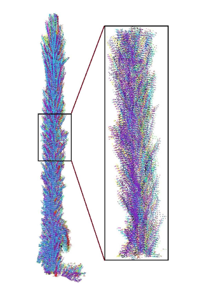
Figure 15: Reconstruction of a conifer plant (different colors indicate different scans).

Figure 16: Growth data for the conifer plant. The conifer as scanned at 14:00 in the afternoon (light) and at 2:00 in the night (dark).

References

- [1] B. Dellen, H. Scharr, and C. Torras, “Growth signatures of rosette plants from time-lapse video,” IEEE/ACM Transactions on Computational Biology and Bioinformatics, vol. 12, no. 6, pp. 1470–1478, 2015.
- [2] T. Dornbusch, S. Lorrain, D. Kuznetsov, A. Fortier, R. Liechti, I. Xenarios, and C. Fankhauser, “Measuring the diurnal pattern of leaf hyponasty and growth in arabidopsis – a novel phenotyping approach using laser scanning,” Functional Plant Biology, vol. 39(11), pp. 860–869, 2012.
- [3] TheArabidopsisGenomeInitiative, “Analysis of the genome sequence of the flowering plant arabidopsis thaliana,” Nature, vol. 408, no. 6814, 2000.
- [4] M. Brophy, “Surface reconstruction from noisy and sparse data,” Ph.D. dissertation, Dept. of Computer Science, University of Western Ontario, December 2015.
- [5] M. Brophy, A. Chaudhury, S. S. Beauchemin, and J. L. Barron, “A method for global nonrigid registration of multiple thin structures,” in Proceedings of the 12th Conference on Computer and Robot Vision (CRV), 2015.
- [6] A. Bucksch and K. Khoshelham, “Localized registration of point clouds of botanic trees,” IEEE Geoscience and Remote Sensing Letters, vol. 10(3), 2013.
- [7] G. Zhou, B. Wang, and J. Zhou, “Automatic registration of tree point clouds from terrestrial lidar scanning for reconstructing the ground scene of vegetated surfaces,” IEEE Geoscience and Remote Sensing Letters, vol. 11, no. 9, pp. 1654–1658, 2014.
- [8] A. Chaudhury, C. Ward, A. Talasaz, A. G. Ivanov, N. P. A. Hüner, B. Grodzinski, R. V. Patel, and J. L. Barron, “Computer vision based autonomous robotic system for 3D plant growth measurement,” in Proc. of 12th conference on Computer and Robot Vision(CRV), 2015.
- [9] E. P. Spalding and N. D. Miller, “Image analysis is driving a renaissance in growth measurement,” Current Opinion in Plant Biology, vol. 16(1), pp. 100–104, 2013.
- [10] A. Hartmann, T. Czauderna, R. Hoffmann, N. Stein, and F. Schreiber, “HTpheno: An image analysis pipeline for high-throughput plant phenotyping,” BMC Bioinformatics, 2011.
- [11] C. Klukas, D. Chen, and J. M. Pape, “Integrated analysis platform: An open-source information system for high-throughput plant phenotyping,” Plant Physiology, vol. 165, no. 2, pp. 506–518, 2014.
- [12] scanalyzer-HTS, http://www.lemnatec.com/products/hardware-solutions/scanalyzer-hts/, 2016.
- [13] R. Subramanian, E. Spalding, and N. Ferrier, “A high throughput robot system for machine vision based plant phenotype studies,” Machine Vision and Applications, vol. 24(3), pp. 619–636, 2013.
- [14] S. Paulus, H. Schumann, H. Kuhlmann, and J. Léon, “High-precision laser scanning system for capturing 3d plant architecture and analysing growth of cereal plants,” Biosystems Engineering, vol. 121, 2014.
- [15] L. Li, Q. Zhang, and D. Huang, “A review of imaging techniques for plant phenotyping,” Sensors, vol. 14, no. 11, 2014.
- [16] R. T. Furbank1 and M. Tester, “Phenomics - technologies to relieve the phenotyping bottleneck,” Trends in Plant Science, vol. 16, no. 12, pp. 635–644, 2011.
- [17] F. Fiorani and U. Schurr, “Future scenarios for plant phenotyping,” Annual Review of Plant Biology, vol. 64, 2013.
- [18] T. Fourcaud, X. Zhang, A. Stokes, H. Lambers, and C. Körner, “Plant growth modelling and applications: The increasing importance of plant architecture in growth models,” Annals of Botany, vol. 101, pp. 1053–1063, 2008.
- [19] A. R. Jiménez, R. C. Ruíz, and J. L. P. Rovira, “A vision system based on a laser range-finder applied to robotic fruit harvesting,” Machine Vision and Applications, vol. 11(6), pp. 321–329, 2000.
- [20] S. Paulus, J. Dupuis, A. K. Mahlein, and H. Kuhlmann, “Surface feature based classification of plant organs from 3D laserscanned point clouds for plant phenotyping,” BMC Bioinformatics, vol. 14, no. 238, 2013.
- [21] S. Paulus, J. Dupuisemail, S. Riedelemail, and H. Kuhlmann, “Automated analysis of barley organs using 3D laser scanning: An approach for high throughput phenotyping,” Sensors, vol. 14(7), pp. 12 670–12 686, 2014.
- [22] M. Klodt, K. Herzog, R. Töpfer, and D. Cremers, “Field phenotyping of grapevine growth using dense stereo reconstruction,” BMC Bioinformatics, vol. 16, p. 143, 2015.
- [23] M. Wahabzada, S. Paulus, K. Kersting, and A. Mahlein, “Automated interpretation of 3d laserscanned point clouds for plant organ segmentation,” BMC Bioinformatics, vol. 16, p. 248, 2015.
- [24] A. Paproki, X. Sirault, S. Berry, R. Furbank, and J. Fripp, “A novel mesh processing based technique for 3D plant analysis,” BMC Plant Biology, vol. 12, no. 1, p. 63, 2012.
- [25] F. Golbach, G. Kootstra, S. Damjanovic, G. Otten, and R. Zedde, “Validation of plant part measurements using a 3D reconstruction method suitable for high-throughput seedling phenotyping,” Machine Vision and Applications, 2015.
- [26] H. Scharr, M. Minervini, A. P. French, C. Klukas, D. M. Kramer, X. Liu, I. Luengo, J. Pape, G. Polder, D. Vukadinovic, X. Yin, and S. A. Tsaftaris, “Leaf segmentation in plant phenotyping: a collation study,” Machine Vision and Applications, vol. 27, no. 4, pp. 585–606, 2016.
- [27] G. Alenyà, B. Dellen, and C. Torras, “3d modelling of leaves from color and tof data for robotized plant measuring,” in IEEE International Conference on Robotics and Automation (ICRA), 2011.
- [28] D. Kelly, A. Vatsa, W. Mayham, and T. Kazic, “Extracting complex lesion phenotypes in zea mays,” Machine Vision and Applications, vol. 27, no. 1, pp. 145–156, 2016.
- [29] G. Xu, F. Zhang, S. G. Shah, Y. Ye, and H. Mao, “Use of leaf color images to identify nitrogen and potassium deficient tomatoes,” Pattern Recognition Letters, vol. 32, no. 11, pp. 1584–1590, 2011.
- [30] E. E. Aksoy, A. Abramov, F. Wörgötter, H. Scharr, A. Fischbach, and B. Dellen, “Modeling leaf growth of rosette plants using infrared stereo image sequences,” Computers and Electronics in Agriculture, vol. 110, pp. 78–90, 2015.
- [31] M. P. Pound, A. P. French, E. H. Murchie, and T. P. Pridmore, “Surface reconstruction of plant shoots from multiple views,” in Proc. of ECCV Workshops, 2014.
- [32] M. P. Pound, A. P. French, J. A. Fozard, E. H. Murchie, and T. P. Pridmore, “A patch-based approach to 3D plant shoot phenotyping,” Machine Vision and Applications, 2016.
- [33] T. T. Santos, L. V. Koenigkan, J. G. A. Barbedo, and G. C. Rodrigues, “3D plant modeling: Localization, mapping and segmentation for plant phenotyping using a single hand-held camera,” in Proc. of ECCV Workshops, 2014.
- [34] T. T. Santos and G. C. Rodrigues, “Flexible three-dimensional modeling of plants using low-resolution cameras and visual odometry,” Machine Vision and Applications, vol. 27, no. 5, pp. 695–707, 2016.
- [35] E. Garnier and A. Berger, “Effect of water stress on stem diameter changes of peach trees growing in the field,” Journal of Applied Ecology, vol. 23(1), pp. 193–209, 1986.
- [36] T. Simonneau, R. Habib, J. Goutouly, and J. Huguet, “Diurnal changes in stem diameter depend upon variations in water content: Direct evidence in peach trees,” Journal of Experimental Botany, vol. 44(3), pp. 615–621, 1992.
- [37] T. Genard, S. Fishman, G. Vercambre, J. Huguet, C. Bussi, J. Besset, and R. Habib, “A biophysical analysis of stem and root diameter variations in woody plants,” Plant Physiology, vol. 126(2), 2001.
- [38] R. Sozzani, W. Busch, E. P. Spalding, and P. N. Benfey, “Advanced imaging techniques for the study of plant growth and development,” Trends in Plant Science, vol. 19, no. 15, 2014.
- [39] P. J. Navarro, C. Fernández, J. Weiss, and . Marcos, “Development of a configurable growth chamber with a computer vision system to study circadian rhythm in plants,” Sensors, vol. 12, no. 11, p. 15356, 2012.
- [40] L. Benoit, D. Rousseau, E. Belin, D. Demilly, and F. Chapeau-Blondeau, “Simulation of image acquisition in machine vision dedicated to seedling elongation to validate image processing root segmentation algorithms,” Computers and Electronics in Agriculture, vol. 104, 2014.
- [41] J. Barron and A. Liptay, “Optic flow to measure minute increments in plant growth,” BioImaging, vol. 2, no. 1, pp. 57–61, 1994.
- [42] A. Liptay, J. L. Barron, T. Jewett, and I. V. Wesenbeeck, “Oscillations in corn seedling growth as measured by optical flow,” Journal of the American Society for Horticultural Science, vol. 120, no. 3, 1995.
- [43] C. Godin and P. Ferraro, “Quantifying the degree of self-nestedness of trees: Application to the structural analysis of plants,” IEEE/ACM Transactions on Computational Biology and Bioinformatics, vol. 7, no. 4, pp. 688–703, 2010.
- [44] M. Augustin, Y. Haxhimusa, W. Busch, and W. G. Kropatsch, “A framework for the extraction of quantitative traits from 2D images of mature arabidopsis thaliana,” Machine Vision and Applications, 2015.
- [45] Y. Li, X. Fan, N. J. Mitra, D. Chamovitz, D. Cohen-Or, and B. Chen, “Analyzing growing plants from 4D point cloud data,” ACM Transactions on Graphics (Proceedings of SIGGRAPH Asia), 2013.
- [46] H. Chui and A. Rangarajan, “A feature registration framework using mixture models,” in Proc. of the IEEE Workshop on Mathematical Methods in Biomedical Image Analysis, ser. MMBIA, 2000.
- [47] Y. Tsin and T. Kanade, “A correlation-based approach to robust point set registration,” in Proc. of 8th European Conference on Computer Vision (ECCV), 2004, pp. 558–569.
- [48] J. Zhang, Z. Huan, and W. Xiong, “An adaptive gaussian mixture model for non-rigid image registration,” Journal of Mathematical Imaging and Vision, vol. 44, no. 3, pp. 282–294, Nov. 2012.
- [49] S. Somayajula, A. A. Joshi, and R. M. Leahy, “Non-rigid image registration using gaussian mixture models,” in Proceedings of the 5th international conference on Biomedical Image Registration, ser. WBIR, 2012, pp. 286–295.
- [50] P. J. Besl and N. D. McKay, “A method for registration of 3D shapes,” IEEE Transactions on Pattern Analysis and Machine Intelligence, vol. 14, no. 2, Feb. 1992.
- [51] G. Turk and M. Levoy, “Zippered polygon meshes from range images,” in Proc. of SIGGRAPH, 1994.
- [52] D. F. Huber and M. Hebert, “Fully automatic registration of multiple 3D data sets,” Image and Vision Computing, vol. 21, no. 7, pp. 637–650, 2003.
- [53] S. Bouaziz, A. Tagliasacchi, and M. Pauly, “Sparce iterative closest point,” Computer Graphics Forum (Symposium on Geometry Processing), vol. 32, no. 5, pp. 1–11, 2013.
- [54] B. Jian and B. C. Vemuri, “Robust point set registration using gaussian mixture models,” IEEE Transactions on Pattern Analysis and Machine Intelligence, vol. 33, no. 8, Aug. 2011.
- [55] A. Myronenko and X. Song, “Point set registration: Coherent point drift,” IEEE Transactions on Pattern Analysis and Machine Intelligence, vol. 32, no. 12, Dec. 2010.
- [56] R. Toldo, A. Beinat, and F. Crosilla, “Global registration of multiple point clouds embedding the generalized procrustes analysis into an ICP framework,” in Proc. of 3DPVT, 2010.
- [57] A. Chaudhury, M. Brophy, and J. L. Barron, “Junction based correspondence estimation of plant point cloud data using subgraph matching,” IEEE Geoscience and Remote Sensing Letters, vol. 13, no. 8, pp. 1119–1123, 2016.
- [58] W. Y. Lin, F. Wang, M. M. Cheng, S. K. Yeung, P. H. S. Torr, M. N. Do, and J. Lu, “Code: Coherence based decision boundaries for feature correspondence,” IEEE Transactions on Pattern Analysis and Machine Intelligence, 2017.
- [59] M. Ester, H. Kriegel, J. Sander, and X. Xu, “A density-based algorithm for discovering clusters in large spatial databases with noise,” in Proc. of International Conference on Knowledge Discovery and Data Mining (KDD), 1996.
- [60] H. Edelsbrunner, D. Kirkpatrick, and R. Seidel, “On the shape of a set of points in the plane,” IEEE Transactions on Information Theory, vol. 29, no. 4, pp. 551–559, 1983.
- [61] C. Zhang and T. Chen, “Efficient feature extraction for 2D/3D objects in mesh representation,” in Proc. of ICIP, 2001.
- [62] D. A. Nusinow, A. Helfer, E. E. Hamilton, J. J. King, T. Imaizumi, T. F. Schultz, E. M. Farré, and S. A. Kay, “The ELF4-ELF3-LUX complex links the circadian clock to diurnal control of hypocotyl growth,” Nature, vol. 475(7356), pp. 398–402, 2011.