Exponential stability in the perturbed central force problem.

Abstract

We consider the spatial central force problem with a real analytic potential. We prove that for all analytic potentials, but the Keplerian and the Harmonic ones, the Hamiltonian fulfills a nondegeneracy property needed for the applicability of Nekhoroshev’s theorem. We deduce stability of the actions over exponentially long times when the system is subject to arbitrary analytic perturbation. The case where the central system is put in interaction with a slow system is also studied and stability over exponentially long time is proved.

1 Introduction and statement of the main result

It is well known that, if the Hamiltonian of an integrable system fulfills some nondegeneracy properties, then Nekhoroshev’s theorem applies and yields strong stability properties of small perturbations of the system [21, 22]. Precisely one gets that the actions are approximately integrals of motions for times exponentially long with the inverse of the size of the perturbation. A sufficient nondegeneracy condition ensuring applicability of Nekhoroshev’s Theorem is quasiconvexity of the Hamiltonian in action-angle coordinates. However, it is nontrivial to prove that in a specific system such a condition is verified, and actually this is known only for a few systems.

In this paper, continuing the investigation of [3], we study the applicability of Nekhoroshev’s theorem to perturbations of the spatial central force problem. The spatial central motion is a superintegrable system that does not admit global action-angle coordinates and moreover its Hamiltonian depends on two actions only. As a consequence it is never quasiconvex in the standard sense. However, modern versions of Nekhoroshev’s theorem [10, 8] apply provided the Hamiltonian is quasiconvex as a function of the two actions on which it actually depends. Here we prove that for any analytic central potential (fulfilling assumptions (H1-H3) below) except the Keplerian and the Harmonic ones, this is the case. Therefore, one gets stability over exponentially long times of these two actions.

To come to a formal statement consider the Hamiltonian of the spatial central force problem in Cartesian coordinates

$$H({\bf x},{\bf p})=\frac{\left|{\bf p}\right|^{2}}{2}+V(|{\bf x}|)\ ,$$ (1.1)

where ${\bf x}\equiv(x,y,z)$, ${\bf p}\equiv(p_{x},p_{y},p_{z})$, $\left|{\bf x}\right|=\sqrt{x^{2}+y^{2}+z^{2}}$ and the potential $V\colon\mathbb{R}_{>0}\to\mathbb{R}$ is a real analytic function satisfying

• $\displaystyle{-\ell^{*}\coloneqq\lim_{r\to 0^{+}}\frac{r^{2}V(r)}{2}>-\infty}$ ;

• $\displaystyle{\exists r>0\,:\,r^{3}V^{\prime}(r)>\max\left\{\,0,\,\ell^{*}\,\right\}}$ ;

• $\forall\ell>\max\left\{\,0,\,\ell^{*}\,\right\}$, $r^{3}V^{\prime}(r)=\ell$ has a finite number of solutions (in $r$).

Remark 1.1.

Assumption (H1) ensures that there exist values of the angular momentum s.t. the effective potential tends to plus infinity as $r\to 0^{+}$, while (H2) ensures that the effective potential has at least one minimum. As a consequence the domain of the action-angle variables is not empty.

These assumptions could be removed and substituted by the assumption that the domain of the action-angle variables is not empty. Here we decided to avoid such a vague assumption, substituting it with some other one, easy to verify and guaranteeing such a condition.

Remark 1.2.

Assumption (H3) is a technical assumption needed in order to simplify the proof of Lemma 4.1 giving the structure of the domain of action-angle variables. We expect that this assumption can be removed.

We denote by ${\bf L}:={\bf x}\times\dot{\bf x}$ the total angular momentum and by $L=|{\bf L}|$ its modulus. Then we consider the perturbed Hamiltonian system

$$H_{\epsilon}=H+\epsilon P\ ,$$

were $P$ is analytic for ${\bf x}\not=0$. For its dynamics the following theorem holds.

Theorem 1.1.

Assume that the potential $V$ fulfills (H1)–(H3) and that it is neither Harmonic nor Keplerian, then there exists a set ${\mathcal{K}}\subset\mathbb{R}^{6}$, which is the union of finitely many analytic hypersurfaces such that: given a compact set ${\mathcal{C}}\subset\mathbb{R}^{6}\setminus{\mathcal{K}}$, invariant for the dynamics of $H$, then there exist positive constants $\epsilon^{*}$, $C_{1}$, $C_{2}$, $C_{3}$ and $C_{4}$ such that, for $|\epsilon|<\epsilon^{*}$ and initial data in ${\mathcal{C}}$, along the dynamics of $H_{\epsilon}$, one has

$$\left|L(t)-L(0)\right|\leq C_{1}\epsilon^{1/4}\ ,\quad\left|H(t)-H(0)\right|\leq C_{2}\epsilon^{1/4}\ ,$$ (1.2)

for

$$\left|t\right|\leq C_{3}\exp(C_{4}\epsilon^{-1/4})\ .$$ (1.3)

Remark 1.3.

The set ${\mathcal{K}}$ is the set where the nondegeneracy assumptions are not fulfilled. In the statement of the theorem we consider a proper subset ${\mathcal{C}}$ in order to obtain values of the nondegeneracy constants independent of the initial datum. A slightly different statement avoiding ${\mathcal{C}}$ is the following one.

Theorem 1.2.

Assume that the potential is neither Harmonic nor Keplerian, then, given an initial datum in $\mathbb{R}^{6}\setminus{\mathcal{K}}$, there exist constants $\epsilon^{*}$, $C_{1}$, $C_{2}$ , $C_{3}$ and $C_{4}$ such that, for $|\epsilon|<\epsilon^{*}$, along the dynamics of $H_{\epsilon}$, the inequalities (1.2) hold for the time (1.3).

An immediate consequence of the above theorem is that, for an exponentially long time, the particle’s orbits are confined between two spherical shells centered at the origin. In addition, in the spirit of [5, 6, 7], in Section 3 we will also give a stability result for the case where the central system is put in interaction with a “slow” system as in models of molecular dynamics [4, 26] (see Theorem 3.2). We will also consider the application to the dynamics of a soliton in NLS [9].

Our result is strongly connected with Bertrand’s theorem, according to which, if all the bounded trajectories of a particle moving under the action of a central force are periodic, then the force is either Keplerian or Harmonic [2, 13]. Actually some steps of our procedure are reminiscent of the classical proof of Bertrand’s theorem, yet our analysis also yields a new proof of a version of Bertrand’s theorem stronger than the classical one (see Appendix A).

We compare now our result to the result of [3]. The present result is stronger than that of [3] in two aspects. First, in [3] the authors proved that non-quasiconvex potentials fulfill a suitable differential equation and that among the homogeneous potentials only the Harmonic and the Keplerian ones fulfill such an equation. Here, through a deeper analysis, we show that all the analytic potential fulfilling assumption (H3) give rise to quasi convex Hamiltonians except the the Harmonic and the Keplerian ones.

Secondly, the result of [3] was only local and the existence of a nondegenerate minimum of the effective potential was explicitly assumed and only initial data belonging to a neighbourhood of such a minimum were considered. On the contrary, we give here a result allowing to deal with any initial datum giving rise to bounded orbits. In particular, since according to our assumptions the effective potential could have local maxima (as in Figure 1), the domain of existence of action-angle variables can have also a connected component not containing a minimum of the potential. The study of this region requires a completely new analysis that is the object of Subsect. 5.3. Making reference to Figure 1, the result of [3] only allows to deal with the regions strictly below $V_{2}$, while here we also deal with the region between $V_{2}$ and $V_{\infty}$.

We now outline the strategy adopted for proving our main result. First we show that the result for the spatial central force problem follows from standard quasiconvexity of the Hamiltonian of the planar central motion. We stress that even if the proof is based on the study of the planar central motion, our main dynamical result, i.e., Theorem 1.1, pertains the spatial case. Of course one can deduce a similar result also for the planar case, but in this case a much stronger result would follow from the application of KAM theory. Indeed, since in systems with two degrees of freedom the KAM tori separate the phase space, their existence implies stability of the actions for all times. Furthermore, the proof of Bertrand’s theorem given in [13] also yields applicability of KAM theorem to all the analytic cases which are neither Harmonic nor Keplerian.

The planar central force problem has two degrees of freedom and the key remark is that for systems with two degrees of freedom quasiconvexity is equivalent to the non vanishing of the Arnold determinant. Furthermore, in an analytic context the Arnold determinant is an analytic function of the actions, therefore only two possibilities occur: either it is a trivial analytic function, or it is always different from zero except on an analytic hypersurface. In Theorem 3.1 we will prove that for the Hamiltonian of the planar central motion such a determinant is a nontrivial function, except in the Keplerian and Harmonic cases.

The study of the Arnold determinant is done via its asymptotics at circular orbits. Precisely, we introduce polar coordinates and recall that the two actions $(I_{1},I_{2})$ of the planar central motion are the modulus of the angular momentum $p_{\theta}\equiv I_{2}$ and the action of the effective system describing the motion of the radial variable

$$H_{{\rm eff}}(r,p_{r},p_{\theta})\coloneqq\frac{p_{r}^{2}}{2}+V_{{\rm eff}}(r,p^{2}_{\theta})\ ,$$ (1.4)

where

$$V_{{\rm eff}}(r,p_{\theta}^{2})\coloneqq V(r)+\frac{p_{\theta}^{2}}{2r^{2}}\ ,$$

and $p_{\theta}$ plays the role of a parameter.

The critical points of the effective potential correspond to circular orbits of the planar system and we show that, except for at most a finite number of values of $p_{\theta}$ that we eliminate, such critical points are nondegenerate. This property is crucial in the subsequent analysis.

The regions where the action $I_{1}$ is defined are open connected regions of the space $(r,p_{r})$, that we denote by ${\mathcal{E}}_{j}$ ($j$ being an index ranging over a finite set), which are constructed as unions of connected components of compact level surfaces of $H$. We distinguish two situations: (1) the closure of ${\mathcal{E}}_{j}$ contains a minimum of the effective potential; (2) the closure of ${\mathcal{E}}_{j}$ does not contain a minimum of the effective potential, thus it must contain a maximum.

First we analyze the regions (1) following the approach adopted in [3]. The idea is to exploit the fact that, for one-dimensional systems, the Birkhoff normal form is convergent close to a nondegenerate minimum of the potential. Thus, at least in principle, one can effectively introduce action-angle variables via Birkhoff normal form and compute the expansion of the Arnold determinant at a minimum. In [3], using the expansion of the Hamiltonian at order two in the actions, it was shown that the zero order term of the Arnold determinant vanishes if and only if the potential fulfills a suitable forth order differential equation. In the present paper, pushing further the expansions with the aid of the Mathematica^TM algebraic manipulator, we expand the Hamiltonian up to order four and we show that the first order term of the Arnold determinant vanishes if the potential fulfills a suitable sixth order differential equation. Finally, still using symbolic manipulation, we show than only the Keplerian and Harmonic potentials satisfy these differential equations. Thus, these are the only two cases in which the expansion of the Arnold determinant at the minimum vanishes.

Second we study the regions (2). Here we compute the asymptotic expansion of the Arnold determinant at the maximum and prove that it is divergent. Thus, if the effective potential has a maximum, then the Hamiltonian is almost everywhere quasiconvex in the region above it. The formula for the behavior of the actions at the maximum has been already obtained by Neishtadt in [20]. Here we give an independent proof based on a normal form result for one dimensional Hamiltonians at saddle points due to Giorgilli [17]. We remark that similar formulæ have also been re-derived by Biasco and Chierchia in [1] for the study of the measure of invariant tori in nearly-integrable systems.

Acknowledgments. We thank Francesco Fassò for suggesting the connection between the result of [3] and the Bertrand’s theorem; Francesco De Vecchi for a hint on the method to find the common solutions of two differential equations; Anatoly Neishtadt for suggesting the formula giving the expansion of the action variable at a maximum, namely (5.8); Luca Biasco for a discussion on the asymptotic expansion of the actions at maxima of the potential and Michela Procesi for suggesting to use our strategy for a new proof of Bertrand’s theorem.

2 Generalized action-angle variables

First of all we recall that in general a superintegrable system does not admit global action-angle variables. This comes from the fact that, in general, the subset of the phase space corresponding to a fixed value of the actions has a nontrivial topology.

A general theory of superintegrable systems has been developed in [10, 11, 18, 19]. Applying such a theory and using the specific form of the Hamiltonian we are going to prove a theorem (Lemma 2.2) giving the structure of the phase space and describing generalized action-angle variables for the spatial central force problem. This is a refinement of Theorems 1 and 2 in [3].

Consider again the Hamiltonian (1.1). In order to define the set where the modulus of the angular momentum varies, we introduce

$$L_{m}^{2} \coloneqq\min\Bigl{\{}\mathbb{R}_{>0}\cap\left[\text{{\rm Range}}(r^{3}V^{\prime}(r))\right]\cap[\ell^{*},+\infty]\Bigr{\}}\ ,$$

$$L_{M} \coloneqq\begin{cases}\sup\sqrt{r^{3}V^{\prime}(r)}\ ,&\text{if }\sup r^{3}V^{\prime}(r)<+\infty\ ;\\ \hat{L}_{M}\ ,&\text{if }\sup r^{3}V^{\prime}(r)=+\infty\ ;\\ \end{cases}$$

where $\hat{L}_{M}$ is an arbitrary large positive number.

The modulus of the angular momentum will be assumed to vary in

$${\mathcal{I}}\coloneqq(L_{m},L_{M})\ .$$

Remark 2.1.

One can think of studying the orbit of the system corresponding to a given initial datum, in the spirit of Theorem 1.2. Correspondingly, having fixed an initial datum giving rise to bounded orbits, one can compute the value of $L_{0}$ of the angular momentum and can take $L_{M}>L_{0}$. Of course one can expect all the constants to deteriorate as $L_{M}$ increases.

The Hamiltonian in action-angle variables has the same form as in the planar case, so to come to a precise statement, which will be useful for the proof of Theorem 1.1, we start to study the planar case.

Consider the planar case and introduce polar coordinates. Then the action variables are $I_{2}:=p_{\theta}$ and the action $I_{1}$ of the effective radial system with Hamiltonian $H_{{\rm eff}}$. The domains of definition of $I_{1}$ are determined by the sublevels of $H_{{\rm eff}}$, which in turn are determined by $V_{{\rm eff}}$. First we want to have stability of the sublevels for small changes of $p_{\theta}$. To this end we will prove that for all values of $p_{\theta}$ except at most a finite number, $V_{{\rm eff}}$ is a Morse function. Thus one gets that ${\mathcal{I}}$ can be decomposed into the union of a finite number of open segments ${\mathcal{I}}_{j}$ plus a finite number of points, with the property that the shape of $V_{{\rm eff}}$ does not change for $p_{\theta}\in{\mathcal{I}}_{j}$ and furthermore all the critical points of $V_{{\rm eff}}$ are nondegenerate. We will show that one can also select the intervals ${\mathcal{I}}_{j}$ in such a way that in such intervals all the critical levels of $V_{{\rm eff}}$ are distinct.

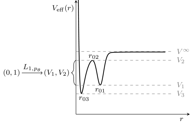
Figure 1: A double-well interaction potential (Lennard-Jones-Gauss).

Then one has to introduce the action $I_{1}$. In order to describe the procedure we make reference to a particular shape depicted in Fig. 1. First we remark that, as $p_{\theta}$ varies in ${\mathcal{I}}_{j}$, the critical points of $V_{{\rm eff}}$ can move, but they cannot cross and their levels cannot cross neither. So, fix an arbitrary value of $p_{\theta}\in{\mathcal{I}}_{j}$. Consider the sublevel $H_{{\rm eff}}<V_{2}$, then the first domain where one can introduce action-angle coordinates is its connected component containing $r_{01}$, to which one has to eliminate the point $(p_{r},r)=(0,r_{01})$. So, such a domain is isomorphic to an interval $E\in(V_{1},V_{2})$ times the level curve $H_{{\rm eff}}=E$. In order to make clear the topological structure of the domains, in the statement of the forthcoming theorem we also introduce an affine map $L_{1,p_{\theta}}$ which transforms the interval $(0,1)$ into $(V_{1},V_{2})$. Of course the map (as well as the target interval) depend on the value of $p_{\theta}$ as well as on the domain identified by the critical point $r_{0i}$ ($r_{01}$ in our case). Then one repeats the construction in all the other domains getting the complete picture.

To give a precise $2-d$ statement, define, for $p_{\theta}\in{\mathcal{I}}$ and arbitrary $E\in\mathbb{R}$,

$${\mathcal{L}}^{(2)}(p_{\theta},E)\coloneqq\bigl{\{}\,(r,p_{r})\,:\,H_{{\rm eff}}(r,p_{r},p_{\theta})=E\,\bigr{\}}\ .$$

As $E\in\mathbb{R}$ and $p_{\theta}\in{\mathcal{I}}$ vary, the sets ${\mathcal{L}}^{(2)}(p_{\theta},E)$ can be empty or can have one or more connected components. For fixed $E$, we enumerate the nonempty compact connected components by ${\mathcal{L}}_{i}^{(2)}(p_{\theta},E)$.

Defining

$${\mathcal{P}}_{A}^{(2)}\coloneqq\left\{(r,p_{r},\theta,p_{\theta})\ :\ \theta\in\mathbb{T}\ ,\ p_{\theta}\in{\mathcal{I}}\ ,\ (r,p_{r})\in\bigcup_{E\in\mathbb{R}}\bigcup_{i}{\mathcal{L}}^{(2)}_{i}(p_{\theta},E)\right\}\ .$$

we have the following lemma.

Lemma 2.1.

There exists a finite number of open intervals ${\mathcal{I}}_{j}$ such that, for any $p_{\theta}\in{\mathcal{I}}_{j}$ there exist a finite number of affine maps, $L_{i,p_{\theta}}\colon(0,1)\to\mathbb{R}$ with the following property: define

$${\mathcal{B}}_{i,j}^{(2)}\coloneqq\left\{(r,p_{r},\theta,p_{\theta})\,:\,\theta\in\mathbb{T}\ ,\ p_{\theta}\in{\mathcal{I}}_{j}\ ,\ (r,p_{r})\in{\mathcal{L}}^{(2)}_{i}(p_{\theta},L_{i,p_{\theta}}{\tt E})\ ,\ {\tt E}\in(0,1)\right\}\ ,$$

and ${\cal S}^{(2)}\coloneqq{\mathcal{P}}_{A}^{(2)}\setminus\bigcup_{i,j}{\mathcal{B}}_{i,j}^{(2)}$; then

• ${\cal S}^{(2)}$ is the union of a finite number of analytic hypersurfaces;

• on each of the domains ${\mathcal{B}}_{i,j}^{(2)}$ there exists an analytic diffeomorphism

  $$\Phi_{i,j}^{(2)}:{\mathcal{B}}_{i,j}^{(2)} \to{\cal A}_{i,j}\times\mathbb{T}^{2}\ ,\qquad{\cal A}_{i,j}\subset\mathbb{R}^{2}$$

  $$(r,p_{r},\theta,p_{\theta}) \mapsto(I_{1},I_{2},\alpha_{1},\alpha_{2})$$

  which introduces action-angle variables;

• for fixed $p_{\theta}\in{\mathcal{I}}_{j}$, the infimum of $H_{{\rm eff}}$ over

  $$\{(r,p_{r})\ :\ (r,p_{r},\theta,p_{\theta})\in{\mathcal{B}}_{i,j}^{(2)}\}$$

  is either a nondegenerate minimum or a nondegenerate maximum of $V_{{\rm eff}}(.;p_{\theta}^{2})$. The function $H_{{\rm eff}}$ has no other critical points in ${\mathcal{B}}_{i,j}^{(2)}$.

This Lemma will be proved in Section 4.

The most important part of the statement, for the proof of Theorem 1.1, is (iii).

Remark 2.2.

In each of the domains ${\mathcal{B}}_{i,j}^{(2)}$ the Hamiltonian, written in terms of the action-angle variables, depends on the actions only. Furthermore it is a function

$$h_{i,j}:{\cal A}_{i,j}\to\mathbb{R}\ ,$$

which is analytic in the whole of ${\cal A}_{i,j}$. This is a simple consequence of the fact that the maps $\Phi_{i,j}^{(2)}$ are analytic diffeomorphisms.

We come now to the three dimensional case.

Given $L\in{\mathcal{I}}$ and arbitrary $E\in\mathbb{R}$, , we define

$${\mathcal{L}}(L,E)\coloneqq\Bigl{\{}({\bf x},{\bf p})\,:\,L^{2}({\bf x},{\bf p})=L^{2}\ \text{and}\ H({\bf x},{\bf p})=E\Bigr{\}}\ .$$

The sets ${\mathcal{L}}(L,E)$ can be empty or can have one or more connected components. As in the $2-d$ case, we denote by ${\mathcal{L}}_{i}(L,E)$ each compact connected component of ${\mathcal{L}}(L,E)$. Define

$${\mathcal{P}}_{A}\coloneqq\bigcup_{L\in{\mathcal{I}}}\bigcup_{E\in\mathbb{R}}\bigcup_{i}{\mathcal{L}}_{i}(L,E)\ .$$

We have the following result

Lemma 2.2.

Corresponding to any domain ${\mathcal{B}}_{i,j}^{(2)}$ of Lemma 2.1, there exists an open set ${\mathcal{B}}_{i,j}\subset{\mathcal{P}}_{A}$, s.t., defining ${\cal S}\coloneqq{\mathcal{P}}_{A}\setminus\bigcup_{i,j}{\mathcal{B}}_{i,j}$ one has

• ${\cal S}$ is the union of a finite number of analytic hypersurfaces;

• each of the domains ${\mathcal{B}}_{i,j}$ can be covered by systems of generalized action-angle coordinates with the same action variables. Precisely, ${\mathcal{B}}_{i,j}$ has the structure of a bifibration

  $${\mathcal{B}}_{i,j}\mathop{\to}^{F_{i,j}}{\mathcal{M}}_{i,j}\mathop{\to}^{\widetilde{F}_{i,j}}{\cal A}_{i,j}\subset\mathbb{R}^{2}\ ,$$

  with the following properties

  • Every fiber of $\displaystyle{{\mathcal{B}}_{i,j}\mathop{\to}^{F_{i,j}}{\mathcal{M}}_{i,j}}$ is diffeomorphic to $\mathbb{T}^{2}$ ;

  • the bifibration is symplectic, i.e., every fiber of $\displaystyle{{\mathcal{B}}_{i,j}\mathop{\to}^{F_{i,j}}{\mathcal{M}}_{i,j}}$ has a neighborhood $U$ endowed with an analytic diffeomorphism

    $$\Phi_{U}:U\to p(U)\times q(U)\times\mathcal{A}_{i,j}\times\mathbb{T}^{2}\ni(p,q,I,\alpha)$$ (2.1)

    such that the level sets of $F_{i,j}$ coincide with the level sets of $p\times q\times I$ and the symplectic form becomes

    $$dp\wedge dq+dI_{1}\wedge d\alpha_{1}+dI_{2}\wedge d\alpha_{2}\ .$$

    The functions $(I_{1},I_{2})$ are globally defined on ${\mathcal{B}}_{i,j}$.

• in each of the domains ${\mathcal{B}}_{i,j}$, the Hamiltonian, as a function of the action variables $(I_{1},I_{2})$, coincides with the Hamiltonian $h_{i,j}$ of the planar central motion in ${\mathcal{B}}_{i,j}^{(2)}$.

3 Statement of the quasiconvexity result and of a further Nekhoroshev type result

Definition 3.1.

Let ${\cal A}\subset\mathbb{R}^{2}$ be open. A function $h\colon{\cal A}\to\mathbb{R}$ is said to be quasiconvex at a point $I^{*}\in{\cal A}$ if

$$\left\{\biggl{\langle}{\eta}\,,\ {\frac{\partial^{2}h}{\partial I^{2}}}(I^{*})\eta\biggr{\rangle}=0\quad\text{and}\quad\biggl{\langle}{{\frac{\partial h}{\partial I}}(I^{*})}\,,\ {\eta}\biggr{\rangle}=0\right\}\ \Longrightarrow\eta=0\ .$$

Our main technical result is the following theorem.

Theorem 3.1.

Assume that the potential $V(r)$ is real analytic and satisfies (H1)–(H3), as in Theorem 1.1, then one of the following two alternatives hold:

• for every $i,j$ there exists at most one analytic hypersurface ${\mathcal{K}}_{i,j}\subset{\cal A}_{i,j}$, s.t. $h_{i,j}$ is quasiconvex for all $(I_{1},I_{2})\in{\cal A}_{i,j}\setminus{\mathcal{K}}_{i,j}$.

• there exists $k>0$ s.t. $V(r)=kr^{2}$ or $V(r)=-k/r$.

Theorem 1.1 immediately follows (see Section 5 for the details).

Remark 3.1.

Both in the Harmonic and the Keplerian cases, the Hamiltonian only depends on one action, thus the steep Nekhoroshev theorem does not apply (see, e.g., [14]).

A remarkable feature of Nekhoroshev’s theorem is that it applies also to the case where the central force problem is in interaction with a further slow system. Let $P\in C^{\omega}({\mathcal{P}}_{A}\times{\mathcal{U}}^{(2n)})$, where ${\mathcal{U}}^{(2n)}\subset\mathbb{R}^{2n}$ is open, and consider the following Hamiltonian with $n+3$ degrees of freedom

$$H_{\epsilon}({\bf x},{\bf p},\widehat{{\bf x}},\widehat{{\bf p}})\coloneqq\frac{1}{\epsilon}H({\bf x},{\bf p})+P({\bf x},{\bf p},\widehat{{\bf x}},\widehat{{\bf p}})\ .$$ (3.1)

This describes, for example, a microscopic central system, so characterized by very light particles subject to very intense forces, interacting with a macroscopic subsystem. For example one could consider $V$ to be the Lennard-Jones potential.

To give a precise statement define

$${\mathcal{E}}(E_{0};{{\bf x}},{{\bf p}})\coloneqq\left\{(\widehat{{\bf x}},\widehat{{\bf p}})\in\mathbb{R}^{2n}\,:\,P({{\bf x}},{{\bf p}},\widehat{{\bf x}},\widehat{{\bf p}})<E_{0}\right\}\ .$$

Theorem 3.2.

Assume that $V(r)$ is neither Harmonic nor Keplerian, let ${\mathcal{C}}$ be fixed as in Theorem 1.1 and let

$${\mathcal{E}}(E_{0})\coloneqq\bigcup_{({{\bf x}},{{\bf p}})\in{\mathcal{C}}}{\mathcal{E}}(E_{0};{{\bf x}},{{\bf p}})\ .$$

Assume that there exists $E_{0}$ such that the function $P$ extends to a bounded analytic function on some complex neighborhood of ${\mathcal{C}}\times{\mathcal{E}}(E_{0})$, then there exist positive $\epsilon^{*}$, $C_{1}$, $C_{2}$, $C_{3}$ and $C_{4}$ with the following property: for $|\epsilon|<\epsilon^{*}$, considering the dynamics of the Hamiltonian system (3.1), then, for any initial datum in ${\mathcal{C}}\times{\mathcal{E}}(E_{0})$ one has that (1.2) hold for the times (1.3).

Remark 3.2.

An interesting different application pertains the dynamics of the soliton of NLS in an external potential. In $\mathbb{R}^{3}$, consider

$${\it i}\dot{\psi}=-\Delta\psi-f^{\prime}(\left|\psi\right|^{2})\psi+\epsilon V\psi\ ,$$ (3.2)

with $V$ a central potential of class Schwartz (the interesting case is that in which it is a potential well) and $f$ a smooth function with a zero of order one at the origin and with the further property that (3.2) admits a stable soliton solution for $\epsilon=0$. It is known (see, e.g., [12]) that when $\epsilon\neq 0$, in first approximation, the soliton moves as a mechanical particle described by the Hamiltonian $H$ with $V$ substituted by a radial effective potential. Then in [9] it was shown that, for times longer then any power of $\epsilon^{-1}$, there is essentially no exchange of energy between the soliton and the rest of the field. Exploiting the result of the present paper one can add Nekhoroshev type techniques in order to show that, for the same time scale and for the majority of initial data, also the angular momentum of the soliton is almost conserved, and thus in particular it does not approach the bottom of the potential well. We avoid here a precise statement, since this would require a quite technical and long preparation.

4 Proof of Lemmas 2.1 and 2.2

We start with the proof of Lemma 2.1. The first point is to show that, except for at most finitely many values of $p_{\theta}\in{\mathcal{I}}$, the effective potential has only nondegenerate critical points and the corresponding critical levels are distinct (see Lemma 4.3).

Remark 4.1.

Due to assumption (H2) there do not exist constants $k_{1},k_{2}$ s.t. the potential has the form

$$V(r)=\frac{k_{1}}{2r^{2}}+k_{2}\ .$$

We also assume $L\not=0$.

Lemma 4.1.

Let $(\bar{r},\bar{\ell})$ be such that $\bar{r}$ is an extremum of $V_{{\rm eff}}(.,\bar{\ell})$. Then there exists an odd $n$, a neighborhood ${\mathcal{U}}$ of $0$ and a function $r_{0}=r_{0}((\ell-\bar{\ell})^{1/n})$ analytic in ${\mathcal{U}}$, s.t. $r_{0}((\ell-\bar{\ell})^{1/n})$ is an extremum of $V_{{\rm eff}}(.;\ell)$. Furthermore $r_{0}(0)=\bar{r}$, and for any $\ell\not=\bar{\ell}$ the extremum is nondegenerate.

Proof.

To fix ideas assume that $\bar{r}$ is a maximum. Of course the theorem holds with $n=1$ if the maximum is nondegenerate. So, assume it is degenerate. Then, since the function $V_{{\rm eff}}(.,\bar{\ell})$ is nontrivial there exists an odd $n>2$, s.t. $\partial_{r}^{n+1}V_{{\rm eff}}(\bar{r},\bar{\ell})=a\not=0$. Thus we look for $\delta=\delta(\xi)$ solving

$$F(\delta,\xi)\coloneqq\partial_{r}V_{{\rm eff}}(\bar{r}+\delta,\bar{\ell}+\xi^{n})=\left[V^{\prime}(\bar{r}+\delta)-\frac{\bar{\ell}}{(\bar{r}+\delta)^{3}}\right]-\frac{\xi^{n}}{(\bar{r}+\delta)^{3}}=0\ .$$ (4.1)

It is convenient to rewrite the square bracket as

$$\frac{a}{n!}\delta^{n}+R_{0}(\delta)\ ,$$

where $R_{0}$ is an analytic function with a zero of order at least $n+1$ at the origin. A short computation shows that we can rewrite (4.1) in the form

$$\delta\left[\left(\frac{a}{n!}+\frac{R_{0}(\delta)}{\delta^{n}}\right)(\bar{r}+\delta)^{3}\right]^{1/n}=\xi\ ,$$ (4.2)

which is in a form suitable for the application of the implicit function theorem. Thus it admits a solution $\delta(\xi)$ which is analytic and which has the form

$$\delta(\xi)=\left(\frac{a}{n!}\bar{r}^{3}\right)^{-1/n}\xi+{\cal O}(\xi^{2})\ .$$

It remains to show that for $\xi$ different from zero (small) the critical point just constructed is nondegenerate. To this end we compute the derivative with respect to $\delta$ of $F$ (c.f. equation (4.1)); we get

$$\partial_{\delta}F(\delta(\xi),\xi) =\frac{a}{(n-1)!}[\delta(\xi)]^{n-1}+R_{0}^{\prime}(\delta(\xi))+\frac{3\xi^{n}}{(\bar{r}+\delta)^{4}}$$ (4.3)

$$=\frac{a}{(n-1)!}\left(\frac{n!}{a\bar{r}^{3}}\right)^{\frac{n-1}{n}}\xi^{n-1}+{\cal O}(\xi^{n})\ ,$$ (4.4)

which for small $\xi$ is non vanishing. ∎

Lemma 4.2.

Let $\bar{r}$ be a degenerate critical point of $V_{{\rm eff}}(.;\bar{\ell})$ which is neither a maximum nor a minimum. Then for $\ell$ in a neighborhood of $\bar{\ell}$, the effective potential $V_{{\rm eff}}(.;\ell)$ either has no critical points in a neighborhood of $\bar{r}$, or it has a nondegenerate maximum and a nondegenerate minimum which depend smoothly on $\ell$.

Proof.

A procedure similar to that used to deduce the equation (4.2) leads to the equation

$$\delta^{n}\left(\frac{a}{n!}+\frac{R_{0}(\delta)}{\delta^{n}}\right)(\bar{r}+\delta)^{3}=\ell-\bar{\ell}\ ,$$

where $n$ is now even and the sign of $a$ is arbitrary. It is thus clear that for $(\ell-\bar{\ell})/a$ negative the critical point disappear. When this quantity is positive then it is easy to see that two new critical points bifurcate from $\bar{r}$. Using a computation similar to that of equations (4.3) and (4.4) one sees that they are a maximum and a minimum which are nondegenerate. ∎

Corollary 4.1.

There exists a finite set ${\mathcal{I}}_{s1}\subset{\mathcal{I}}$ such that, $\forall p_{\theta}\in{\mathcal{I}}\setminus{\mathcal{I}}_{s1}$ the effective potential $V_{{\rm eff}}(.;p_{\theta}^{2})$ has only critical points which are nondegenerate extrema.

Proof.

Just remark that the values of $p_{\theta}$ for which $V_{{\rm eff}}(.;p_{\theta}^{2})$ has at least one degenerate critical point are isolated. Thus, due to the compactness of $\overline{{\mathcal{I}}}$ their number is finite. ∎

Remark 4.2.

The set ${\mathcal{I}}\setminus{\mathcal{I}}_{s1}$ is the union of finitely many open intervals. The critical points of $V_{{\rm eff}}$ are analytic functions of $p_{\theta}^{2}$ in such intervals; furthermore they do not cross (at crossing points their multiplicity would be greater then one, against nondegeneracy). Therefore the number, the order and the nature of the critical points is constant in each of the subintervals.

The main structural result we need for the effective potential is the following

Lemma 4.3.

There exists a finite set ${\mathcal{I}}_{s}\subset{\mathcal{I}}$ such that, $\forall p_{\theta}\in{\mathcal{I}}\setminus{\mathcal{I}}_{s}$ the effective potential $V_{{\rm eff}}(.;p_{\theta}^{2})$ has only critical points which are nondegenerate extrema and the critical levels are all distinct. Furthermore each critical level does not coincide with

$$V^{\infty}\coloneqq\lim_{r\to\infty}V(r)\ .$$

Proof.

First we restrict to ${\mathcal{I}}\setminus{\mathcal{I}}_{s1}$, so that all the critical points of $V_{{\rm eff}}$ are nondegenerate. We concentrate on one of the open subintervals of ${\mathcal{I}}\setminus{\mathcal{I}}_{s1}$ (cf. Remark 4.2). Let $\ell\coloneqq p_{\theta}^{2}$, and let $r(\ell)$ be a critical point of $V_{{\rm eff}}(.;\ell)$. Consider the corresponding critical level $V_{{\rm eff}}(r(\ell),\ell)$ and compute

$$\frac{d}{d\ell}V_{{\rm eff}}(r(\ell),\ell)=\frac{\partial r}{\partial\ell}\frac{\partial V_{{\rm eff}}}{\partial r}(r(\ell),\ell)+\frac{\partial V_{{\rm eff}}}{\partial\ell}=\frac{1}{2r^{2}}\ ,$$ (4.5)

where we used the fact that $r(\ell)$ is critical, so that $\frac{\partial V_{{\rm eff}}}{\partial r}(r(\ell),\ell)=0$ and the explicit expression of $V_{{\rm eff}}$ as a function of $\ell$. Thus the derivative (4.5) depends on $r$ only. It follows that if two critical levels coincide, then their derivatives with respect to $\ell$ are different, and therefore they become different when $\ell$ is changed. It follows that also the set of the values of $\ell$ for which some critical levels coincide is formed by isolated points, and therefore it is composed by at most a finite number of points in each subinterval. Of course a similar argument applies to the comparison with $V^{\infty}$.∎

We are now ready for the construction of action-angle variables (and the proof of Lemma 2.1). Consider one of the connected subintervals of ${\mathcal{I}}\setminus{\mathcal{I}}_{s}$ and denote it by $\widetilde{{\mathcal{I}}}$. We distinguish two cases: (1) the effective potential has no local maxima for $p_{\theta}\in\widetilde{{\mathcal{I}}}$; (2) the effective potential has at least one local maximum for $p_{\theta}\in\widetilde{{\mathcal{I}}}$.

We start by the case (1). The second action is $I_{2}\coloneqq p_{\theta}$, while the first one is given by

$$I_{1}=G(E,I_{2})\coloneqq\frac{1}{\pi}\int_{r_{min}}^{r_{max}}\!\!\!\sqrt{2(E-V_{{\rm eff}}(r;I_{2}^{2}))}dr\ ,\quad E\in(V_{{\rm eff}}(r_{0};I_{2}^{2}),V^{\infty})\ ,$$ (4.6)

where $r_{min}$ and $r_{max}$ are the solutions of the equation $E=V_{{\rm eff}}(r;I_{2}^{2})$ and $r_{0}$ is the minimum of the potential. Correspondingly the action $I_{1}$ varies in $(0,G(V^{\infty},I_{2}))$. Thus the domain $\widetilde{{\mathcal{B}}}^{(2)}$ is

$$\widetilde{{\mathcal{B}}}^{(2)}\coloneqq\left\{(r,p_{r},\theta,p_{\theta})\,:\,p_{\theta}\in\widetilde{{\mathcal{I}}}\ ,(r,p_{r})\in\bigcup_{E\in(V_{{\rm eff}}(r_{0};I_{2}^{2}),V^{\infty})}{\mathcal{L}}^{(2)}(p_{\theta},V^{\infty})\right\}\ ,$$

and the actions vary in

$$\widetilde{{\cal A}}\coloneqq\left\{(I_{1},I_{2})\,:\,I_{2}\in\widetilde{{\mathcal{I}}}\ ,\ I_{1}\in(0,G(V^{\infty},I_{2}))\right\}\ .$$

In this domain the Hamiltonian is computed by computing $E$ as a function of $I_{1},I_{2}$ by inverting the function $G$ defined in (4.6).

In this case we define the affine map $\widetilde{L}_{p_{\theta}}$ of Lemma 2.1 by

$$\widetilde{L}_{p_{\theta}}{\tt E}\coloneqq\left[V^{\infty}-V_{{\rm eff}}(r_{0}(p_{\theta}^{2});p_{\theta}^{2})\right]{\tt E}+V_{{\rm eff}}(r_{0}(p_{\theta}^{2});p_{\theta}^{2})\ .$$ (4.7)

We consider now the case where the effective potential has at least one local maximum. In this case, in general, there are several different domains which are described by action-angle coordinates. To fix ideas consider the case where $V_{{\rm eff}}(.;p_{\theta}^{2})$ has exactly two minima $r_{01}>r_{03}$ and one maximum $r_{02}$ fulfilling $V_{{\rm eff}}(r_{02};I_{2}^{2})<V^{\infty}$ (as in Fig. 1). Then the level sets ${\mathcal{L}}(p_{\theta},E)$, for $V_{{\rm eff}}(r_{03};I_{2}^{2})<E<V_{{\rm eff}}(r_{02};I_{2}^{2})$ have two connected components, in each of which one can construct the action variables exactly by the formula (4.6) (with a suitable redefinition of $r_{min}$ and ${r_{max}}$).

Then there is a further domain in which the action $I_{1}$ can be defined; it corresponds to the level sets with $V_{{\rm eff}}(r_{02};I_{2}^{2})<E<V^{\infty}$ above the local maximum. In this domain the action is still given by the formula (4.6). It is clear that in more general situations only one more kind of domains of the phase space can exists: namely domains in which both the minimal energy and the maximal energy correspond to the energies of local maxima of the effective potential, but in this case the construction goes exactly in the same way.

Summarizing we have that the following

Lemma 4.4.

Each of the domains ${\mathcal{B}}_{i,j}^{(2)}$ in which a system of action-angle variables is defined is the union for $I_{2}$ in an open interval, say ${\mathcal{I}}_{j}$ of level sets of $H_{{\rm eff}}$. The infimum over ${\mathcal{B}}^{(2)}_{i,j}$ of the energy $H_{{\rm eff}}$ is either a nondegenerate maximum or a nondegenerate minimum of the effective potential. The corresponding value of the radius will be denoted by $r_{0j}=r_{0j}(I^{2}_{2})$ and depends analytically on $I_{2}\in{\mathcal{I}}_{j}$.

Proof of Lemma 2.1. So we have constructed action-angle variables in a domain excluding the following sets, which we define ${\cal S}^{(2)}$ and which are analytic hypersurfaces:

• $\displaystyle{\left\{(r,p_{r},\theta,p_{\theta})\ :\ p_{\theta}=0\right\}}$  ;

• $\displaystyle{\left\{(r,p_{r},\theta,p_{\theta})\ :\ p_{\theta}\in{\mathcal{I}}_{s}\right\}}$  ;

• $\displaystyle{\left\{(r,p_{r},\theta,p_{\theta})\ :\ V_{0j}(p_{\theta})=H(r,p_{r},p_{\theta})\right\}}$ .

where we denoted

$$V_{0j}(I_{2})\coloneqq V_{{\rm eff}}(r_{0j}(I_{2}^{2}),I_{2}^{2})=V(r_{0j})+\frac{r_{0j}V^{\prime}(r_{0j})}{2}\ ,$$

the corresponding critical level. ∎

Proof of Lemma 2.2. First we fix a couple of indexes $i,j$ as in the Lemma 2.1, and, for $L\in{\mathcal{I}}_{i}$ and $E\in L_{i,L}(0,1)$, define

$${\mathcal{L}}_{i,j}(L,E)\coloneqq\bigl{\{}\,({\bf x},{\bf p})\ :\ L^{2}({\bf x},{\bf p})=L^{2}\ \text{and}\ H({\bf x},{\bf p})=E\,\bigr{\}}\ .$$

Then simply define ${\mathcal{B}}_{i,j}\coloneqq\bigcup_{L\in{\mathcal{I}}_{j}}{\mathcal{L}}_{i,j}(L,E)$. By the Lemma 2.1 it is clear that the assumptions of Theorem 1 in [11] are fulfilled and the results on the structure of the phase space holds. To get that the Hamiltonian has the same form as in the planar case, just remark that the whole phase-space can be covered using two systems of polar coordinates with $z$-axis ($\theta=0$) not coinciding. Using any one of the two systems, one can introduce explicitly, by the classical procedure, action-angle variables which turn out to be $I_{2}=L$ and $I_{1}$ which is the action of the Hamiltonian system with $1$ degree of freedom and Hamiltonian $H(r,p_{r},L^{2})$. Thus, $I_{1}$ has exactly the same expression as in the planar case, but with $p_{\theta}^{2}$ replaced by $L^{2}$.

It follows that the Hamiltonian which is computed by inversion of the formula for $I_{1}$ has the same functional form as in the planar case. ∎

5 Proof of Theorem 3.1.

From Lemma 2.2, it follows that it is enough to consider the planar case; so we now study such a case.

5.1 The quasiconvexity condition

Before going to the heart of the proof we give a couple of equivalent forms of the quasiconvexity condition. Consider a Hamiltonian $h\colon{\cal A}\to\mathbb{R}$, with ${\cal A}\subset\mathbb{R}^{2}$, with two degrees of freedom, in action variables and define

$$\omega_{1}={\frac{\partial h}{\partial I_{1}}}\ ,\quad\omega_{2}={\frac{\partial h}{\partial I_{2}}}\ .$$

It is well-known that that considering systems with two degrees of freedom quasiconvexity is equivalent to the non vanishing of the Arnold determinant (see, e.g., [3]), namely

$$\mathcal{D}=\det\begin{pmatrix}{\dfrac{\partial^{2}h}{\partial I^{2}}}&\left({\dfrac{\partial h}{\partial I}}\right)^{T}\ \\ {\dfrac{\partial h}{\partial I}}&0\end{pmatrix}\ ,$$

that explicitly reads

$$\mathcal{D}=-\frac{\partial^{2}h}{\partial I_{1}^{2}}\omega_{2}^{2}+2\frac{\partial^{2}h}{\partial I_{1}\partial I_{2}}\omega_{1}\omega_{2}-\frac{\partial^{2}h}{\partial I_{2}^{2}}\omega_{1}^{2}\ .$$

Thus, rearranging the terms appearing in $\mathcal{D}$, it is straightforward to see that, if $\omega_{2}$ does not vanish, the condition $\mathcal{D}=0$ can be written as a Burgers equation,

$${\frac{\partial\nu}{\partial I_{1}}}=\nu{\frac{\partial\nu}{\partial I_{2}}}\ ,\quad\hbox{with }\nu=\frac{\omega_{1}}{\omega_{2}}\ ,$$ (5.1)

which is a form convenient for the study of ${\mathcal{D}}$ close to a minimum of the effective potential. It is easy to see that, provided $L\not=0$, close to a minimum of the effective potential $\omega_{2}$ does not vanish.

5.2 Domains bounded below by a minimum

In this section we concentrate on domains ${\mathcal{B}}_{i,j}^{(2)}$ such that the infimum of the energy $H$ at fixed $I_{2}$ is a minimum of the effective potential. In particular the minimum $r_{0j}$ of the effective potential is nondegenerate. In this section, since the domain is fixed, we omit the index $j$ from the various quantities. Thus ${\cal A}$ will be the domain of the actions, $h$ the Hamiltonian written in action variables, $r_{0}$ the minimum of the effective potential and $V_{0}$ the corresponding value.

The main result of this section is the following

Lemma 5.1.

Let ${\mathcal{B}}_{i,j}^{(2)}$ be a domain where the infimum of the effective Hamiltonian at fixed $I_{2}$ is a nondegenerate minimum of the effective potential. Assume that the Arnold determinant vanishes in an open subset of ${\mathcal{B}}_{i,j}^{(2)}$, then the potential is either Keplerian or Harmonic.

The rest of the section is devoted to the proof of such Lemma.

As explained in the introduction we exploit the remark that in one-dimensional analytic systems the Birkhoff normal form converges in a (complex) neighborhood of a nondegenerate minimum. This, together with the essential uniqueness of the action variables in one-dimensional systems, implies that, for any $I_{2}$, the Hamiltonian $h$, as a function of $I_{1}$, extends to a complex analytic function in a neighborhood of $I_{1}=0$ and that the expansion constructed through the one-dimensional Birkhoff normal form is actually the expansion of $h(I_{1},I_{2})$ at $I_{1}=0$. It follows that also ${\mathcal{D}}$ extends to a complex analytic function of $I_{1}$ in a neighborhood of 0. Thus one has an expansion

$$h(I_{1},I_{2})=h_{0}(I_{2})+h_{1}(I_{2})I_{1}+\ldots+h_{n}(I_{2})I_{1}^{n}+\ldots\ ,$$

where the quantities $h_{n}$ can be in principle computed as functions of the derivatives of $V$ at $r_{0}(I_{2})$ and of $I_{2}$.

Here we will proceed by an explicit construction using a symbolic manipulator. We recall that explicit computations of Birkhoff normal forms have already been implemented numerically in different context (see, e.g., [23, 15, 16] in the context of the $n$-body problem, and [24, 25] for the spin-orbit problem). We refer to that works for the details about the implementation of the Birkhoff normal form. We only stress that here the main difference consists in the fact that all the parameters are represented by symbols and the coefficients are rational numbers: thus the Birkhoff normal form is computed in exactly and without any numerical approximation.

Remark 5.1.

In ${{\mathcal{B}}_{i,j}^{(2)}}$ there is a 1-1 correspondence between $I_{2}$ and $r_{0}$, so each of the functions $h_{n}$ can be considered just as a function of $r_{0}$ and of the derivatives of $V$ at $r_{0}$. Correspondingly the derivatives with respect to $I_{2}$ can be converted into derivatives with respect to $r_{0}$ through the rule

$${\frac{\partial}{\partial I_{2}}}=\frac{2}{(3+g(r_{0}))\sqrt{r_{0}V^{\prime}(r_{0})}}\,{\frac{\partial}{\partial r_{0}}}\ ,$$ (5.2)

where, following the notation introduced in [3], we have defined

$$g(r_{0})\coloneqq\frac{{r_{0}}V^{\prime\prime}({r_{0}})}{V^{\prime}({r_{0}})}\ .$$ (5.3)

Furthermore, it is convenient to define

$$R(r_{0},V^{\prime}(r_{0}),g(r_{0}))\coloneqq\frac{2}{(3+g(r_{0}))\sqrt{r_{0}V^{\prime}(r_{0})}}\ .$$ (5.4)

Remark 5.2.

The condition that the function $g$ is constant is equivalent to the fact that the potential is homogeneous or logarithmic, precisely, one has

$$g(r_{0})=c\quad\iff\quad\begin{cases}V(r)=\frac{k}{c+1}r^{c+1}\,,\ k\in\mathbb{R}\setminus\left\{0\right\}&\text{if}\ c\not=-1\\ V(r)=k\ln r\,,\ k\in\mathbb{R}\setminus\left\{0\right\}&\text{if}\ c=-1\end{cases}$$

Then one can use the expansion obtained through the Birkhoff normal form to compute the expansion of $\nu\equiv\omega_{1}/\omega_{2}$ at the minimum, namely

$$\nu(I_{1},I_{2})=\nu_{0}(I_{2})+\nu_{1}(I_{2})I_{1}+\ldots+\nu_{n}(I_{2})I_{1}^{n}+\ldots\ .$$ (5.5)

Remark 5.3.

Since the frequency is the derivative of the Hamiltonian with respect to the action, in order to compute $\nu_{j}$ one has to know the Birkhoff normal form at order $2(j+1)$ in the Cartesian variables, which correspond to know the expansion of the Birkhoff normal form at order $j+1$ in $I_{1}$.

The idea is now to impose that the Burgers equation (5.1) is satisfied up to the first order in $I_{1}$ identically as function of $I_{2}$, namely to impose

$$\begin{aligned} \nu_{1}&=\nu_{0}{\frac{\partial\nu_{0}}{\partial I_{2}}}\ ,\\ \nu_{2}&=\frac{1}{2}\left(\nu_{1}{\frac{\partial\nu_{0}}{\partial I_{2}}}+\nu_{0}{\frac{\partial\nu_{1}}{\partial I_{2}}}\right)\ ,\end{aligned}$$ (5.6)

and to consider such equations as the ones determining the degenerate potentials. We will show that such equations admit the only common solutions given by the Harmonic and the Keplerian potential. Of course a degenerate Hamiltonian fulfills also higher order equations, but they are not relevant for our result.

According to Remark 5.1, we will consider all the $\nu_{j}$ as functions of $r_{0}$ instead of $I_{2}$ and convert all the derivatives with respect to $I_{2}$ into derivatives with respect to $r_{0}$ by using (5.2).

Finally, it is convenient to use, as much as possible, $g$ as an independent variable (see (5.3)) instead of $V$. We remark that $V^{\prime\prime}({r_{0}})={g(r_{0})V^{\prime}({r_{0}})}/{r_{0}}$, which implies that $\forall n\geq 2$ the $n$-th derivative of the potential can be expressed as a function of $r_{0},V^{\prime}(r_{0}),g(r_{0}),g^{\prime}(r_{0}),\ldots,g^{(n-2)}(r_{0})$. We will systematically do this.

There is a remarkable fact: writing explicitly the equations (5.6), it turns out that they are independent of $V^{\prime}$, thus they are only differential equations for $g$.

We report below the outline of the computations and the key formulæ. The symbolic manipulations have been implemented in Mathematica™and are available upon request to the authors.

Remark 5.4.

Let us stress that in principle all the calculations could be done without resorting to algebraic manipulation on a computer. We just made use of symbolic manipulations because the expressions become soon too cumbersome. We emphasize that no approximations are involved in the manipulations, since all the coefficients are rational numbers.

Firstly we computed explicitly $\nu_{0}$, $\nu_{1}$ and $\nu_{2}$, defined by (5.5), getting

$$\nu_{0} =\sqrt{3+g(r_{0})}\ ,$$

$$\nu_{1} =\nu_{1}(r_{0},V^{\prime}(r_{0}),g(r_{0}),g^{\prime}(r_{0}),g^{\prime\prime}(r_{0}))\ ,$$

$$\nu_{2} =\nu_{2}(r_{0},V^{\prime}(r_{0}),g(r_{0}),g^{\prime}(r_{0}),g^{\prime\prime}(r_{0}),g^{(3)}(r_{0}),g^{(4)}(r_{0}))\ .$$

The explicit forms of $\nu_{1}$ and $\nu_{2}$ are rather long and are reported in the Appendix B.

Secondly we can use the explicit forms of the functions $\nu_{0}$ and $\nu_{1}$ so as to compute the r.h.s. of (5.6), which will have the form

$$R\nu_{0}{\frac{\partial\nu_{0}}{\partial r_{0}}} =:G_{1}(r_{0},V^{\prime}(r_{0}),g(r_{0}),g^{\prime}(r_{0}))\ ,$$

$$\frac{1}{2}R\left(\nu_{1}{\frac{\partial\nu_{0}}{\partial r_{0}}}+\nu_{0}{\frac{\partial\nu_{1}}{\partial r_{0}}}\right) =:G_{2}(r_{0},V^{\prime}(r_{0}),g(r_{0}),g^{\prime}(r_{0}),g^{\prime\prime}(r_{0}),g^{(3)}(r_{0}))\ ,$$

where $R$ is the expression defined in (5.4).

Lastly, imposing $\nu_{1}=G_{1}$ and $\nu_{2}=G_{2}$, we get two differential equations for $g$ that we are going to solve. Let us stress that the first one is exactly the equation for $g$ appearing in Remark 3 of [3].

The strategy, in order to find the common solutions, consists in taking derivatives of the equation of lower order until one gets two equations of the same order (forth order in $g$ in our case), then one solves one of the equations for the higher order derivative and substitutes it in the other one, thus getting an equation of order smaller then the previous one; then one iterates. In our case the final equation will be an algebraic equation for $g$, whose solutions are just constants. The value of such constants correspond to the Kepler and the Harmonic potentials, so the conclusion will hold.

In detail, we solve $\nu_{1}=G_{1}$ for $g^{\prime\prime}(r_{0})$ and $\nu_{2}=G_{2}$ for $g^{(4)}(r_{0})$, getting

$$g^{\prime\prime}(r_{0}) =f_{2}(r_{0},g(r_{0}),g^{\prime}(r_{0}))\ ,$$ (5.7)

$$g^{(4)}(r_{0}) =f_{4}(r_{0},g(r_{0}),g^{\prime}(r_{0}),g^{(3)}(r_{0}))\ ,$$

where, in the second one, we also used $f_{2}(r_{0},g(r_{0}),g^{\prime}(r_{0}))$ to remove the dependence of $g^{(4)}$ on $g^{\prime\prime}(r_{0})$. A similar procedure will be done systematically.

Starting from (5.7), we compute

$${\frac{{\rm d}^{2}f_{2}}{{\rm d}r_{0}^{2}}}=F_{4}(r_{0},g(r_{0}),g^{\prime}(r_{0}),g^{(3)}(r_{0}))\ ,$$

and solve the equation $F_{4}(r_{0},g(r_{0}),g^{\prime}(r_{0}),g^{(3)}(r_{0}))=f_{4}(r_{0},g(r_{0}),g^{\prime}(r_{0}),g^{(3)}(r_{0}))$ for $g^{(3)}$, getting

$$g^{(3)}=f_{3}(r_{0},g(r_{0}),g^{\prime}(r_{0}))\ .$$

Starting again from (5.7), we compute

$${\frac{{\rm d}f_{2}}{{\rm d}r_{0}}}=F_{3}(r_{0},g(r_{0}),g^{\prime}(r_{0}))\ ,$$

and solve the equation $F_{3}(r_{0},g(r_{0}),g^{\prime}(r_{0}))=f_{3}(r_{0},g(r_{0}),g^{\prime}(r_{0}))$ for $g^{\prime}$ getting

$$g^{\prime}=f_{1}(r_{0},g(r_{0}))\ .$$

Finally we compute

$${\frac{{\rm d}f_{1}}{{\rm d}r_{0}}}=F_{2}(r_{0},g(r_{0}))\ ,$$

and solve $F_{2}(r_{0},g(r_{0}))=f_{2}(r_{0},g(r_{0}))$ for $g$. It is remarkable that such an equation turns out to be independent of $r_{0}$, so that the solutions for $g(r_{0})$ are just isolated points, namely constants. In [3] it was already shown that the only constants solving $\nu_{1}=G_{1}$ are $-3,-2$ and $1$. The value $-3$ is excluded according to Remark 4.1, therefore the only remaining potentials are the Keplerian and the Harmonic ones. This concludes the proof of Lemma 5.1.

5.3 Domains bounded below by a maximum

Consider now domains ${\mathcal{B}}_{i,j}^{(2)}$ s.t. the infimum of the energy $H$ at a fixed $I_{2}\in\widetilde{{\mathcal{I}}}$ is a nondegenerate maximum of the effective potential $V_{{\rm eff}}$. Denote by $V_{0}=V_{0}(I_{2})$ the value of the effective potential at such a maximum delimiting from below the range of the energy in ${\mathcal{B}}_{i,j}^{(2)}$.

Lemma 5.2.

Let ${\mathcal{B}}_{i,j}^{(2)}$ be a domain s.t. the infimum of the effective Hamiltonian at fixed $I_{2}$ is a nondegenerate maximum of the effective potential, then the Arnold determinant vanishes in ${\mathcal{B}}_{i,j}^{(2)}$ at most on an analytic hypersurface.

The rest of the section is devoted to the proof of such a lemma. The main tool for studying the limiting behavior of the action close to the maximum $V_{0}$ is the following normal form theorem, which is a slight reformulation of a simplified version of the main result in [17].

Theorem 5.1.

Let

$$W(r)=W_{0}-\frac{\lambda^{2}}{2}r^{2}+\mathcal{O}(r^{3})$$

be an analytic potential having a nondegenerate maximum at $r=0$; consider the Hamiltonian

$$H(r,p_{r})=\frac{p_{r}^{2}}{2}+W(r)$$

then, there exists an open neighborhood ${\mathcal{V}}_{0}$ of $0$ and a near to identity canonical transformation $\Phi:{\mathcal{V}}_{0}\ni(x,y)\mapsto(r,p_{r})\in{\mathcal{U}}_{0}\coloneqq\Phi({\mathcal{V}}_{0})$ of the form

$$\left\{\begin{aligned} r&=\frac{x}{\sqrt{\lambda}}+f_{1}(x,y)\\ p_{r}&=\sqrt{\lambda}y+f_{2}(x,y)\end{aligned}\right.$$

with $f_{1},f_{2}$ analytic functions which are at least quadratic in $x,y$ and such that the Hamiltonian takes the form

$$h(x,y)=W_{0}+\lambda J+\sum_{i\geq 1}\lambda_{i}J^{i+1}\ ,\qquad J\coloneqq\frac{y^{2}-x^{2}}{2}\ .$$

Furthermore, the series is convergent in $\mathcal{V}_{0}$.

The behavior of the action variable close to the maximum of the effective potential is described by the following

Theorem 5.2.

Let $\bar{E}=E-V_{0}(I_{2})$, then there exist two functions $\Lambda(\bar{E},I_{2})$, $G_{1}\left(\bar{E},I_{2}\right)$ such that the first action $I_{1}$ is given by

$$I_{1}=G(\bar{E},I_{2})\coloneqq-\Lambda(\bar{E},I_{2})\ln\bar{E}+G_{1}\left(\bar{E},I_{2}\right)\ .$$ (5.8)

Furthermore $\Lambda$ and $G_{1}$ are bounded in the domain

$$\left\{(\bar{E},I_{2})\ :\ I_{2}\in\widetilde{\mathcal{I}}\ ,\ \bar{E}\in[0,V_{M}(I_{2})-V_{0}(I_{2}))\right\}\ ,$$ (5.9)

where $V_{M}(I_{2})$ is the maximal value of the energy at fixed $I_{2}$ in ${\mathcal{B}}_{i,j}^{(2)}$ and analytic in its interior. Finally one has

$$\Lambda(\bar{E},I_{2})\coloneqq\frac{\bar{E}+\mathcal{F}(\bar{E},I_{2})}{\pi\lambda(I_{2})}\ ,$$

with $\mathcal{F}$ having a zero of order $2$ in $(0,I_{2})$ and $\lambda^{2}=\lambda^{2}(I_{2})\coloneqq-\frac{d^{2}V_{{\rm eff}}}{dr^{2}}(r_{0})>0$.

Remark 5.5.

The main point is that the lower extremum of the interval (5.9) for $\bar{E}$ is included, thus (5.8) describes the actions until the maximum. Furthermore, by (5.8) the limit

$$I_{1\,0}\coloneqq\lim_{\bar{E}\rightarrow 0^{+}}G(\bar{E},I_{2})=G_{1}(0,I_{2})$$

exists and is finite.

Remark 5.6.

Since $E\mapsto G(E-V_{0}(I_{2}),I_{2})$ is a monotonically increasing function for $E\in(V_{0}(I_{2}),V_{M}(I_{2}))$, there exists a function $h(I_{1},I_{2})$ such that

$$G(h(I_{1},I_{2})-V_{0}(I_{2}),I_{2})\equiv I_{1}\ .$$

Furthermore, by the implicit function theorem, $h$ is analytic in $I_{1},I_{2}$ for $I_{2}\in\widetilde{{\mathcal{I}}}$ and $I_{1}>I_{1\,0}$.

Proof of Theorem 5.2. Let $I_{2}\in\widetilde{{\mathcal{I}}}$ and consider the Hamiltonian (1.4) with $p_{\theta}=I_{2}$. In the whole construction $I_{2}$ will play the role of a parameter, thus we will omit the dependence on $I_{2}$ and just consider the $(r,p_{r})$ dependence.

Firstly, expanding at $r_{0}$, we obtain

$$H(r,p_{r})=\frac{p_{r}^{2}}{2}+V_{0}-\frac{\lambda^{2}}{2}(r-r_{0})^{2}+\mathcal{O}\left((r-r_{0})^{3}\right)\ .$$

Secondly, via the change of variable $r^{\prime}\coloneqq r-r_{0}$, (omitting the primes) we get

$$H(r,p_{r})=\frac{p_{r}^{2}}{2}+V_{0}-\frac{\lambda^{2}}{2}r^{2}+\mathcal{O}(r^{3})\ .$$

Fix a value of the energy $E>V_{0}$, close enough to $V_{0}$ and denote by $\gamma(E)$ the level curve corresponding to $H=E$. Thus we have

$$I_{1}=\frac{1}{2\pi}\int_{\gamma(E)}p_{r}dr=\frac{1}{\pi}\int_{\gamma^{+}(E)}p_{r}dr$$

where $\gamma^{+}(E)$ is the upper part of the level curve, namely, $\gamma|_{p_{r}>0}$.

We split the domain of integration into two regions, precisely

$$I_{1}=\frac{1}{\pi}\left[\int_{\gamma^{+}(E)\,\cap\,\mathcal{U}}p_{r}dr+\int_{\gamma^{+}(E)\,\cap\,\mathcal{U}^{c}}p_{r}dr\right]\ .$$ (5.10)

where $\mathcal{U}$ is a neighborhood of the nondegenerate maximum that will be fixed in a while. First, we remark that the second integral does not see the critical point, so it is an analytic function of $E$ until $V_{0}$. To analyze the first integral, we exploit Theorem 5.1.

Let us fix a small positive $x_{1}$ and let us consider the neighborhood ${\mathcal{V}}$ of 0 defined by

$$\mathbb{R}^{2}\supset\mathcal{V}\coloneqq(-x_{1},x_{1})\times\left(-\sqrt{\frac{4\bar{E}}{\lambda}+x_{1}^{2}},\sqrt{\frac{4\bar{E}}{\lambda}+x_{1}^{2}}\right)\ .$$

Provided $\bar{E}$ and $x_{1}$ are small enough, one has $\mathcal{V}\subset\mathcal{V}_{0}$ (c.f. Theorem 5.1). Let us define ${\mathcal{U}}\coloneqq\Phi(\mathcal{V})$ and write $\gamma_{+}(E)\cap{\mathcal{U}}$ in the variables $(x,y)$, parametrizing it with $x\in(-x_{1},x_{1})$. To this end remark that, since the Hamiltonian $H$ is a function of $J$ only, namely

$$H=V_{0}+\lambda J+\mathcal{G}(J)$$

where $\mathcal{G}(J)=\sum_{i\geq 1}\lambda_{i}J^{i+1}$, by the implicit function theorem, there exists an analytic function ${\mathcal{F}}(\bar{E})$ having a zero of order $2$ at $0$ and such that

$$J=\frac{\bar{E}+{\mathcal{F}}(\bar{E})}{\lambda}$$

and, therefore, $\gamma_{+}(E)$ can be written in the form $(x,y(x))$ with

$$y(x)\coloneqq\sqrt{\frac{2(\bar{E}+{\mathcal{F}}(\bar{E}))}{\lambda}+x^{2}}\ .$$

To compute the first integral in (5.10), we remark that since $\Phi$ is canonical and analytic in a neighborhood of the origin, there exists a function $S(x,y)$, analytic in a neighborhood of the origin, such that

$$p_{r}dr=ydx+dS\ ,$$

thus, we have

$$\int_{\gamma_{+}(E)\cap{\mathcal{U}}}p_{r}dr=\int_{-x_{1}}^{x_{1}}ydx+S(x_{1},y(x_{1}))-S(-x_{1},y(-x_{1}))\ .$$

Since $x_{1}$ is fixed, the terms involving $S$ are analytic functions of $\bar{E}$. Thus, we only compute the first integral, namely,

$$\int_{-x_{1}}^{x_{1}}ydx=\int_{-x_{1}}^{x_{1}}\sqrt{\frac{2(\bar{E}+{\mathcal{F}}(\bar{E},I_{2}))}{\lambda}+x^{2}}dx$$

which takes the form

$$\int_{-x_{1}}^{x_{1}}ydx =\frac{2(\bar{E}+{\mathcal{F}}(\bar{E}))}{\lambda}\ln\left(x_{1}+\sqrt{x_{1}^{2}+\frac{2(\bar{E}+{\mathcal{F}}(\bar{E}))}{\lambda}}\right)$$

$$\qquad+x_{1}\sqrt{x_{1}^{2}+\frac{2(\bar{E}+{\mathcal{F}}(\bar{E}))}{\lambda}}$$

$$\qquad-\frac{\bar{E}+{\mathcal{F}}(\bar{E})}{\lambda}\ln\left(\frac{2(\bar{E}+{\mathcal{F}}(\bar{E}))}{\lambda}\right).$$

It is easy to see that the first two terms are analytic in a neighborhood of $0$.

Rewriting the third term as

$$-\frac{\bar{E}+{\mathcal{F}}(\bar{E})}{\lambda}\ln\bar{E}-\ln\left(\frac{2}{\lambda}+\frac{2{\mathcal{F}}(\bar{E})}{\bar{E}}\right)$$

and remarking that the second function is analytic in a neighborhood of $0$, we get the result. Formula (5.8) is obtained by reinserting the dependence on $I_{2}$. ∎

We come now to the Arnold determinant. Firstly, we will work in the region $\bar{E}>0$ so that the function $G$ is regular and the implicit function theorem applies and allows to compute $h$ and its derivatives. Then, we will study the limit $\bar{E}\rightarrow 0^{+}$.

By the implicit function theorem, the frequency $\omega_{1}$ is given by

$$\omega_{1}={\frac{\partial h}{\partial I_{1}}}=\left({\frac{\partial G}{\partial\bar{E}}}\right)^{-1}=:{\mathcal{W}}_{1}(\bar{E},I_{2})\ .$$ (5.11)

Remark 5.7.

Let $f$ be an analytic function of the form

$$f=f(\bar{E},I_{2})=f(h(I_{1},I_{2})-V_{0}(I_{2}),I_{2})\ ,$$

then,

$${\frac{{\rm d}f}{{\rm d}I_{2}}}\coloneqq{\frac{\partial f}{\partial\bar{E}}}{\frac{\partial\bar{E}}{\partial I_{2}}}+{\frac{\partial f}{\partial I_{2}}}={\frac{\partial f}{\partial\bar{E}}}\left(\omega_{2}-{\frac{\partial V_{0}}{\partial I_{2}}}\right)+{\frac{\partial f}{\partial I_{2}}}.$$

It follows from Remark 5.7 and the implicit function theorem that the frequency $\omega_{2}$ is given by

$$\omega_{2}={\frac{\partial h}{\partial I_{2}}}=-{\frac{\partial G}{\partial I_{2}}}{\mathcal{W}}_{1}+{\frac{\partial V_{0}}{\partial I_{2}}}.$$

Thus, it is worth introducing a function ${\mathcal{W}}_{2}$ defined by

$${\mathcal{W}}_{2}(\bar{E},I_{2})\coloneqq-{\frac{\partial G}{\partial I_{2}}}{\mathcal{W}}_{1}+{\frac{\partial V_{0}}{\partial I_{2}}}.$$ (5.12)

Proposition 5.1.

Let $h\colon\mathcal{A}\rightarrow\mathbb{R}$ be the Hamiltonian in two degrees of freedom written in action-angle coordinates, then the Arnold determinant can be rewritten in terms of $G$ and ${\mathcal{W}}_{1}$ as

$${{\mathcal{D}}}=-{\mathcal{W}}_{1}{\frac{\partial{\mathcal{W}}_{1}}{\partial\bar{E}}}\left({\frac{\partial V_{0}}{\partial I_{2}}}\right)^{2}+2{\mathcal{W}}_{1}{\frac{\partial{\mathcal{W}}_{1}}{\partial I_{2}}}{\frac{\partial V_{0}}{\partial I_{2}}}+{\mathcal{W}}_{1}^{3}{\frac{\partial^{2}G}{\partial I_{2}^{2}}}-{\mathcal{W}}_{1}^{2}{\frac{\partial^{2}V_{0}}{\partial I_{2}^{2}}}$$ (5.13)

Proof.

By exploiting the formulæ (5.11), (5.12) and Remark 5.7, we compute the second derivatives of the Hamiltonian $h$. We have

$${\frac{\partial^{2}h}{\partial I_{1}^{2}}} ={\frac{\partial{\mathcal{W}}_{1}(\bar{E},I_{2})}{\partial I_{1}}}={\frac{\partial{\mathcal{W}}_{1}}{\partial\bar{E}}}{\frac{\partial h}{\partial I_{1}}}={\mathcal{W}}_{1}{\frac{\partial{\mathcal{W}}_{1}}{\partial\bar{E}}}$$

$$\frac{\partial^{2}h}{\partial I_{1}\partial I_{2}} ={\frac{{\rm d}{\mathcal{W}}_{1}(\bar{E},I_{2})}{{\rm d}I_{2}}}$$

$${\frac{\partial^{2}h}{\partial I_{2}^{2}}} ={\frac{{\rm d}{\mathcal{W}}_{2}(\bar{E},I_{2})}{{\rm d}I_{2}}}={\frac{{\rm d}}{{\rm d}I_{2}}}\left(-{\mathcal{W}}_{1}{\frac{\partial G}{\partial I_{2}}}+{\frac{\partial V_{0}}{\partial I_{2}}}\right)$$

$$=-{\frac{{\rm d}{\mathcal{W}}_{1}}{{\rm d}I_{2}}}{\frac{\partial G}{\partial I_{2}}}-{\mathcal{W}}_{1}{\frac{{\rm d}}{{\rm d}I_{2}}}\left({\frac{\partial G}{\partial I_{2}}}\right)+{\frac{\partial^{2}V_{0}}{\partial I_{2}^{2}}}$$

We can write the three terms of the Arnold determinant separately as

$${{\mathcal{D}}_{1}}=-{\mathcal{W}}_{1}{\mathcal{W}}_{2}^{2}{\frac{\partial{\mathcal{W}}_{1}}{\partial\bar{E}}},$$ (5.14)

$${{\mathcal{D}}_{2}}=2{\mathcal{W}}_{1}{\mathcal{W}}_{2}{\frac{{\rm d}{\mathcal{W}}_{1}}{{\rm d}I_{2}}},$$ (5.15)

$${{\mathcal{D}}_{3}}={\mathcal{W}}_{1}^{2}{\frac{\partial G}{\partial I_{2}}}{\frac{{\rm d}{\mathcal{W}}_{1}}{{\rm d}I_{2}}}+{\mathcal{W}}_{1}^{3}{\frac{{\rm d}}{{\rm d}I_{2}}}\left({\frac{\partial G}{\partial I_{2}}}\right)-{\mathcal{W}}_{1}^{2}{\frac{\partial^{2}V_{0}}{\partial I_{2}^{2}}}.$$ (5.16)

And, gathering together the expressions (5.14), (5.15) and (5.16), after simple computation, we obtain

$${{\mathcal{D}}}=-{\mathcal{W}}_{1}{\frac{\partial{\mathcal{W}}_{1}}{\partial\bar{E}}}\left({\frac{\partial V_{0}}{\partial I_{2}}}\right)^{2}+2{\mathcal{W}}_{1}{\frac{\partial{\mathcal{W}}_{1}}{\partial I_{2}}}{\frac{\partial V_{0}}{\partial I_{2}}}+{\mathcal{W}}_{1}^{3}{\frac{\partial^{2}G}{\partial I_{2}^{2}}}-{\mathcal{W}}_{1}^{2}{\frac{\partial^{2}V_{0}}{\partial I_{2}^{2}}}$$

This concludes the proof. ∎

Proposition 5.2.

The Arnold determinant diverges as $\bar{E}$ tends to zero.

Proof.

Due to the structure (5.8) of $G$, it is easy to see that ${\frac{\partial^{2}G}{\partial I_{2}^{2}}}$ is bounded as $\bar{E}\rightarrow 0^{+}$ (remark that ${\frac{\partial G}{\partial I_{2}}}$ means derivative with respect to the second argument). Therefore, since ${\frac{\partial^{2}V_{0}}{\partial I_{2}^{2}}}$ is a regular function of $I_{2}$ and ${\mathcal{W}}_{1}\rightarrow 0$ as $\bar{E}$ approaches zero, we have that

$$\lim_{\bar{E}\rightarrow 0^{+}}\left({\mathcal{W}}_{1}^{3}{\frac{\partial^{2}G}{\partial I_{2}^{2}}}-{\mathcal{W}}_{1}^{2}{\frac{\partial^{2}V_{0}}{\partial I_{2}^{2}}}\right)=0.$$

Let us now concentrate on the analysis of the remaining terms of (5.13). The asymptotic behavior of the function ${\mathcal{W}}_{1}$ is given by

$${\mathcal{W}}_{1}\sim-\frac{\pi\lambda}{\ln\bar{E}}.$$

Concerning the derivatives, we have

$${\frac{\partial{\mathcal{W}}_{1}}{\partial I_{2}}}=-\left({\frac{\partial G}{\partial\bar{E}}}\right)^{-2}\frac{\partial^{2}G}{\partial I_{2}\partial\bar{E}}\mathop{\to}^{\bar{E}\rightarrow 0^{+}}0\quad\Longrightarrow\quad\lim_{\bar{E}\rightarrow 0^{+}}\left(2{\mathcal{W}}_{1}{\frac{\partial{\mathcal{W}}_{1}}{\partial I_{2}}}{\frac{\partial V_{0}}{\partial I_{2}}}\right)=0\ .$$

Concerning the first term, using

$${\frac{\partial{\mathcal{W}}_{1}}{\partial\bar{E}}}\sim\frac{\pi\lambda}{\bar{E}\ln^{2}\bar{E}}\ ,$$

we have that it behaves as

$$\frac{\pi^{2}\lambda^{2}}{\bar{E}\ln^{3}\bar{E}}\left({\frac{\partial V_{0}}{\partial I_{2}}}\right)^{2}$$

which diverges to infinity as $\bar{E}\rightarrow 0^{+}$. This concludes the proof. ∎

Lemma 5.2 follows from the fact that ${\mathcal{D}}$ is a nontrivial analytic function in ${\cal A}_{i,j}$.

Appendix A A new proof of Bertrand’s Theorem

We give here a new proof of Bertrand’s Theorem. Actually we give here a local version of the Theorem (in the spirit of [13]). The obtained result is slightly stronger then the usual one.

Theorem A.1 (Bertrand).

Consider the planar central force problem with an analytic potential $V$ s.t. a stable circular orbit exists. Denote by $\gamma$ the phase space trajectory of such a circular orbit. If there exists a neighborhood of $\gamma$ in which all the orbits are periodic then the potential is either Keplerian or Harmonic.

Proof.

First remark that a stable circular orbit is a minimum of the effective potential corresponding to a particular value of the angular momentum. By modifying the value of the angular momentum (according to Lemma 4.1) one reduces to the case where the minimum is nondegenerate. Consider now the quantity ${\frac{\partial\nu}{\partial I_{1}}}-\nu{\frac{\partial\nu}{\partial I_{2}}}$: in Section 5.1 we proved that it vanishes identically only in the Keplerian and in the Harmonic cases. Assume by contradiction that this is not the case. Then ${\frac{\partial\nu}{\partial I_{1}}}-\nu{\frac{\partial\nu}{\partial I_{2}}}$ is a nontrivial function of the actions, and thus the ratio $\nu(I_{1},I_{2})\equiv\frac{\omega_{1}}{\omega_{2}}$ is also a non-constant function. It follows that there exist $I_{1},I_{2}$ such that $\nu$ is irrational and thus on the corresponding torus the motion is not periodic, against the assumption. ∎

Appendix B A couple of formulæ

We report here for completeness the explicit formulæ of the functions introduced in the proof of Lemma 5.1.

$$\nu_{1}= \Bigl{(}36+9{r_{0}}^{2}g^{\prime\prime}({r_{0}})-g({r_{0}})^{2}\left({r_{0}}g^{\prime}({r_{0}})+26\right)+g({r_{0}})\left(3{r_{0}}^{2}g^{\prime\prime}({r_{0}})+7{r_{0}}g^{\prime}({r_{0}})+6\right)$$

$$\ +30{r_{0}}g^{\prime}({r_{0}})-5{r_{0}}^{2}g^{\prime}({r_{0}})^{2}-2g({r_{0}})^{4}-14g({r_{0}})^{3}\Bigr{)}\Big{/}\left(24{r_{0}}^{3/2}(g({r_{0}})+3)^{2}\sqrt{V^{\prime}({r_{0}})}\right)\ ,$$

$$\nu_{2}= \Bigl{(}-235{r_{0}}^{4}g^{\prime}({r_{0}})^{4}+2604{r_{0}}^{3}g^{\prime}({r_{0}})^{3}+4g({r_{0}})^{6}\left(17{r_{0}}g^{\prime}({r_{0}})+759\right)$$

$$\ +g({r_{0}})^{5}\left(-84{r_{0}}^{2}g^{\prime\prime}({r_{0}})+600{r_{0}}g^{\prime}({r_{0}})+13408\right)+54{r_{0}}^{2}g^{\prime}({r_{0}})^{2}\left(25{r_{0}}^{2}g^{\prime\prime}({r_{0}})-142\right)$$

$$\ -27\left(17{r_{0}}^{4}g^{\prime\prime}({r_{0}})^{2}-456{r_{0}}^{2}g^{\prime\prime}({r_{0}})-24\left({r_{0}}^{4}g^{(4)}({r_{0}})+12{r_{0}}^{3}g^{(3)}({r_{0}})-62\right)\right)$$

$$\ +g({r_{0}})^{4}\left(-48{r_{0}}^{3}g^{(3)}({r_{0}})-1344{r_{0}}^{2}g^{\prime\prime}({r_{0}})+129{r_{0}}^{2}g^{\prime}({r_{0}})^{2}+624{r_{0}}g^{\prime}({r_{0}})+33500\right)$$

$$\ -108{r_{0}}g^{\prime}({r_{0}})\left(14{r_{0}}^{3}g^{(3)}({r_{0}})+101{r_{0}}^{2}g^{\prime\prime}({r_{0}})+260\right)$$

$$\ +2g({r_{0}})^{3}\Bigl{(}699{r_{0}}^{2}g^{\prime}({r_{0}})^{2}+{r_{0}}g^{\prime}({r_{0}})\left(81{r_{0}}^{2}g^{\prime\prime}({r_{0}})-4732\right)$$

$$\ +12\left({r_{0}}^{4}g^{(4)}({r_{0}})-6{r_{0}}^{3}g^{(3)}({r_{0}})-296{r_{0}}^{2}g^{\prime\prime}({r_{0}})+1705\right)\Bigr{)}$$

$$\ -g({r_{0}})^{2}\Bigl{(}94{r_{0}}^{3}g^{\prime}({r_{0}})^{3}-4053{r_{0}}^{2}g^{\prime}({r_{0}})^{2}+3\Bigl{(}17{r_{0}}^{4}g^{\prime\prime}({r_{0}})^{2}+4680{r_{0}}^{2}g^{\prime\prime}({r_{0}})$$

$$\ -36\left(2{r_{0}}^{4}g^{(4)}({r_{0}})+12{r_{0}}^{3}g^{(3)}({r_{0}})+11\right)\Bigr{)}$$

$$\ +12{r_{0}}g^{\prime}({r_{0}})\left(14{r_{0}}^{3}g^{(3)}({r_{0}})+20{r_{0}}^{2}g^{\prime\prime}({r_{0}})+3291\right)\Bigr{)}$$

$$\ +2g({r_{0}})\Bigl{(}293{r_{0}}^{3}g^{\prime}({r_{0}})^{3}+9{r_{0}}^{2}g^{\prime}({r_{0}})^{2}\left(25{r_{0}}^{2}g^{\prime\prime}({r_{0}})+28\right)$$

$$\ -9\left(-36{r_{0}}^{4}g^{(4)}({r_{0}})-360{r_{0}}^{3}g^{(3)}({r_{0}})+17{r_{0}}^{4}g^{\prime\prime}({r_{0}})^{2}+198{r_{0}}^{2}g^{\prime\prime}({r_{0}})+2904\right)$$

$$\ -9{r_{0}}g^{\prime}({r_{0}})\left(56{r_{0}}^{3}g^{(3)}({r_{0}})+323{r_{0}}^{2}g^{\prime\prime}({r_{0}})+3216\right)\Bigr{)}$$

$$\ +20g({r_{0}})^{8}+376g({r_{0}})^{7}\Bigr{)}\Big{/}\Bigl{(}2304{r_{0}}^{3}(g({r_{0}})+3)^{9/2}V^{\prime}({r_{0}})\Bigr{)}\ .$$

References

- BC [17] L. Biasco and L. Chierchia. KAM Theory for secondary tori. ArXiv e-prints, February 2017.
- Ber [73] J. Bertrand. Théorèm relatif au mouvement d’un point attiré vers un centre fixe. Comptes Rendus, 77:849–853, 1873.
- BF [17] D. Bambusi and A. Fusè. Nekhoroshev theorem for perturbations of the central motion. Regul. Chaotic Dyn., 22(1):18–26, 2017.
- BG [93] D. Bambusi and A. Giorgilli. Exponential stability of states close to resonance in infinite-dimensional hamiltonian systems. J. Stat. Phys., 71(3-4):569–606, 1993.
- BGG [87] G. Benettin, L. Galgani and A. Giorgilli. Realization of holonomic constraints and freezing of high frequency degrees of freedom in the light of classical perturbation theory. I. Comm. Math. Phys., 113(1):87–103, 1987.
- BGG [89] G. Benettin, L. Galgani and A. Giorgilli. Realization of holonomic constraints and freezing of high frequency degrees of freedom in the light of classical perturbation theory. II. Comm. Math. Phys., 121(4):557–601, 1989.
- BGPP [13] D. Bambusi, A. Giorgilli, S. Paleari and T. Penati. Normal form and energy conservation of high frequency subsystems without nonresonance conditions. Rendiconti dell’Istituto Lombardo Accademia di Scienze e Lettere, Classe di Scienze Matematiche e Naturali, 147:1–17, 2013.
- Bla [01] A. D. Blaom. A geometric setting for Hamiltonian perturbation theory. Number 727. American Mathematical Soc., 2001.
- BM [16] D. Bambusi and A. Maspero. Freezing of energy of a soliton in an external potential. Communications in Mathematical Physics, 344(1):155–191, 2016.
- Fas [95] F. Fassò. Hamiltonian perturbation theory on a manifold. Celestial Mechanics and Dynamical Astronomy, 62(1):43–69, 1995.
- Fas [05] F. Fassò. Superintegrable Hamiltonian systems: geometry and perturbations. Acta Applicandae Mathematica, 87(1-3):93–121, 2005.
- FGJS [04] J. Fröhlich, S. Gustafson, B. L. G. Jonsson and I. M. Sigal. Solitary wave dynamics in an external potential. Comm. Math. Phys., 250(3):613–642, 2004.
- FK [04] J. Féjoz and L. Kaczmarek. Sur le théorème de Bertrand (d’après Michael Herman). Ergodic Theory and Dynamical Systems, 24(05):1583–1589, 2004.
- GCB [16] M. Guzzo, L. Chierchia and G. Benettin. The steep Nekhoroshev’s theorem. Comm. Math. Phys., 342(2):569–601, 2016.
- GLS [14] A. Giorgilli, U. Locatelli and M. Sansottera. On the convergence of an algorithm constructing the normal form for elliptic lower dimensional tori in planetary systems Celestial Mechanics and Dynamical Astronomy, 119(3-4):397–424, 2014.
- GLS [17] A. Giorgilli, U. Locatelli and M. Sansottera. Secular dynamics of a planar model of the Sun-Jupiter-Saturn-Uranus system; effective stability in the light of Kolmogorov and Nekhoroshev theories, Regular and Chaotic Dynamics, 22(1):54–77, 2017.
- Gio [01] A. Giorgilli. Unstable equilibria of Hamiltonian systems. Discrete Contin. Dynam. Systems, 7(4):855–871, 2001.
- KM [12] M. V. Karasev and V. P. Maslov. Nonlinear Poisson brackets: geometry and quantization, volume 119. American Mathematical Soc., 2012.
- MF [78] A.S. Mishchenko and A.T. Fomenko. Generalized liouville method of integration of hamiltonian systems. Functional analysis and its applications, 12(2):113–121, 1978.
- Nei [87] AI Neishtadt. On the change in the adiabatic invariant on crossing a separatrix in systems with two degrees of freedom. Journal of Applied Mathematics and Mechanics, 51(5):586–592, 1987.
- Nek [77] N.N. Nekhoroshev Exponential estimates of the stability time of near-integrable Hamiltonian systems. Russ. Math. Surveys, 32:1–65, (1977).
- Nek [79] N.N. Nekhoroshev Exponential estimates of the stability time of near-integrable Hamiltonian systems, 2. Trudy Sem. Petrovs., 5:5–50, (1979).
- SLG [13] M. Sansottera, U. Locatelli and A. Giorgilli. On the stability of the secular evolution of the planar Sun-Jupiter-Saturn-Uranus system. Mathematics and Computers in Simulation, 88:1–14, 2013.
- SLL [14] M. Sansottera, Christoph Lhotka and A. Lemaître. Effective stability around the Cassini state in the spin-orbit problem. Celestial Mechanics and Dynamical Astronomy, 119(1):75–89, 2014.
- SLL [15] M. Sansottera, C. Lhotka and A. Lemaître. Effective resonant stability of mercury. Monthly Notices of the Royal Astronomical Society, 452(4):4145, 2015.
- Teu [03] S. Teufel. Adiabatic perturbation theory in quantum dynamics, volume 1821 of Lecture Notes in Mathematics. Springer-Verlag, Berlin, 2003.