A Non-Intrusive Parallel-in-Time Adjoint Solver with the XBraid Library

Abstract

In this paper, an adjoint solver for the multigrid-in-time software library XBraid is presented. XBraid provides a non-intrusive approach for simulating unsteady dynamics on multiple processors while parallelizing not only in space but also in the time domain xbraid-package . It applies an iterative multigrid reduction in time algorithm to existing spatially parallel classical time propagators and computes the unsteady solution parallel in time. Techniques from Automatic Differentiation are used to develop a consistent discrete adjoint solver which provides sensitivity information of output quantities with respect to design parameter changes. The adjoint code runs backwards through the primal XBraid actions and accumulates gradient information parallel in time. It is highly non-intrusive as existing adjoint time propagators can easily be integrated through the adjoint interface. The adjoint code is validated on advection-dominated flow with periodic upstream boundary condition. It provides similar strong scaling results as the primal XBraid solver and offers great potential for speeding up the overall computational costs for sensitivity analysis using multiple processors.

1 Introduction

With the rapid increase in computational capacities, computational fluid dynamics (CFD) has nowadays become a powerful tool to predict and analyze steady and unsteady fluid flows. For unsteady dynamics, a numerical CFD simulation approximates the state $u(t)$ of a dynamical system (e.g. density, velocity or temperature), given problem specific design parameters denoted by $\rho$ (such as geometry, boundary and initial conditions or material coefficients), while the state is determined through a set of unsteady partial differential equations (PDEs):

$$\frac{\mathrm{d}u(t)}{\mathrm{d}t} =g(u(t),\rho)\quad\forall t\in(0,T)$$ (1)

$$u(0) =g^{0}.$$ (2)

Here, the right hand side $g$ involves spatial derivatives, source terms, etc. as well as the design parameters $\rho$. Accounting for the unidirectional flow of information in the time domain, an approximation to the unsteady PDE solution is typically evolved forward in time in a step-by-step manner applying a time marching algorithm blazek2005computational ; Peric:2002 ; tucker2014unsteady . Starting from the initial condition, these schemes march forward in discrete time steps applying nonlinear iterations in space to approximate a pseudo-steady state at each time step as for example in the dual-time stepping approach jameson1991dualtime .

However, in many applications, the primal flow is not the only computation of particular interest. The ability to compute sensitivities is also needed to determine the influence of design changes to some objective function $J$ that computes the time-average of instantaneous quantities of the flow dynamics

$$J(u,\rho)=\frac{1}{T}\int_{0}^{T}f(u(t),\rho)\mathrm{d}t.$$ (3)

The ability to compute sensitivities can improve and enhance the simulation tool, as for example through parameter estimation for validation and verification purposes navon1998practical , error estimation and adaptive grid refinement venditti2002grid ; pierce2000adjoint ; giles2002adjoint or uncertainty quantification techniques beyer2007robust . Further, it broadens the application range from pure simulation to optimization as for example in an optimal control or shape optimization framework jameson1988aerodynamicdesign ; nadarajah2007optimum ; mohammadi2010applied .

If the number of independent design parameters is large, the adjoint approach for sensitivity computations is usually preferred since its computational cost does not scale with the design space dimension pironneau_1974 ; giles1997adjoint . In that approach, only one additional adjoint equation needs to be solved in order to set up the gradient of the objective function $J$ with respect to $\rho$. For unsteady time marching schemes, solving the adjoint equation involves a reverse time integration loop that propagates sensitivities backwards through the time domain starting from a terminal condition nadarajah2007optimum ; economon2013unsteady ; rumpfkeil2007general ; mavriplis2008solution ; nielsen2010discrete . Hence evaluating the gradient is a rather computationally expensive task as it involves a forward loop over the time domain to approximate the PDE solution followed by a backwards time marching loop for the adjoint.

One way to mitigate this costly procedure of forward and backward sweeps over the time domain is to parallelize the time dimension. Overall, the need for parallel-in-time methods is being driven by changes in computer architectures, where future speedups will be available through greater concurrency, not faster clock speeds, which are stagnant. Previously, ever faster clock speeds made it possible to speedup fixed-size sequential time stepping problems (strong scaling), and also to refine problems in time and space without increasing the wall-clock time (weak scaling). However with stagnate clock speeds, speedups will only be possible through the increasing concurrency of future architectures. Thus, to overcome this serial time stepping bottleneck, time stepping codes must look for new parallelism from the time dimension. This bottleneck is particularly acute for adjoint solvers because of the many sweeps over the time domain.

Research on parallel-in-time methods goes at least back to the 1964 work by Nievergelt Nievergelt_1964 . Since then, a variety of approaches have been developed, including parareal, which is perhaps the most popular parallel-in-time method parareal-2001 . For a recent literature review and a gentle introduction, see Ga2015 . The method used here is multigrid reduction in time (MGRIT) and is based on multigrid reduction mgrit-2014 ; ries_trottenberg_1979_mgr ; ries_etal_1983_mgr . MGRIT is relatively non-intrusive on existing codes and when restricted to two grid levels, is equivalent to parareal mgrit-2014 ; GV_2007_parareal . This multilevel distinction is important, because it allows for optimal parallel communication behavior, as opposed to a two-level scheme, where the size of the coarse-level limits concurrency. This work uses XBraid, an open source implementation of MGRIT developed at Lawrence Livermore National Lab xbraid-package .

Previous time parallel approaches to optimization include multiple shooting methods He2005 , parareal approaches applied to a reduced Hessian DuSaSch2005 ; mathew2010analysis , and the Schwarz preconditioner approaches in BaSt2015 ; KwGa2016 ; kwok2017time . Further, GoetschelMinion2017 uses the time-parallel PFASST approach to solve the state and adjoint equations for parabolic optimal control problems. While these previous approaches were effective, applying XBraid for optimization offers some possible advantages, e.g., XBraid offers multilevel scalability, and the potential for greater parallelism over the Schwarz approaches. The parallelism for the Schwarz approaches is limited by the size of fine-grid “subdomains” which must each be solved sequentially, but for XBraid, the size of such subdomains is determined by the temporal coarsening factor, which can be as small as 2.

When considering the intersection of optimization, CFD, and parallel-in-time, a prerequisite is that parallel-in-time be effective for standard fluid dynamics problems, and recent advances indicate that parallel-in-time can indeed be an effective tool here. In FarCha2003 , the Parallel Implicit Time-Integration Algorithm (PITA) was proposed, which enjoys success for highly advective problems, targeting in part fluid dynamics RuKr2012 . It essentially uses a parareal framework, but creates a massive Krylov space to stabilize and accelerate the method. While effective, the memory usage of this algorithm is discouraging. When considering unmodified parareal, the works FiHeMa2005 ; SteRuSpKr2015 ; RuKr2014 show that parareal can be effective for fluids problems when sufficient physical (not artificial) diffusion is present. Similar success with XBraid was shown for vortex shedding FalKatz2014 . Lastly, the work Do2016 showed a path forward for XBraid and purely advective problems that relies only on artificial dissipation.

The XBraid package will be presented in Section 2. Section 3 reviews the adjoint approach for computing sensitivities. Then, in Section 4, an approach to modifying XBraid in order to integrate existing adjoint time stepping codes into the XBraid framework is developed. Exploiting techniques from Automatic Differentiation (AD) griewank2008evaluating , the primal XBraid iterations are enhanced by an adjoint iteration that runs backwards through the XBraid actions and computes consistent discrete adjoint sensitivities. Similar to the primal XBraid solver, the resulting adjoint solver is non-intrusive in the sense that existing adjoint simulation codes can easily be integrated through the extended user interface. Finally, the adjoint code is validated in Section 5 by applying it to advection-dominated flow with a periodic upstream boundary.

2 Multigrid Reduction in Time using XBraid

To describe the MGRIT algorithm implemented by XBraid, let $u(t)$ be the solution to a time-dependent problem on the interval $[0,T]$. Let $t_{i}=i\delta t,i=0,1,...,N$ be a time grid of that interval with spacing $\delta t=T/N$, and let $\vec{u}^{i}\in\mathbb{R}^{n}$ be an approximation of $u(t_{i})$.

Classical time marching schemes successively compute $\vec{u}^{i}$ based on information at previous time steps $\vec{u}^{i-1},\vec{u}^{i-2},\dots,$ and the design $\rho$ where $\rho\in\mathbb{R}^{p}$ in a discretized setting. Implicit methods are often prefered due to better stability properties leading to nonlinear equations at each time step that need to be solved iteratively for $\vec{u}^{i}$. Wrapping these iterations into a time stepper $\Phi^{i}\colon\mathbb{R}^{n}\times\mathbb{R}^{p}\to\mathbb{R}^{n}$, a general one-step time marching scheme can be written as

$$\vec{u}^{i}=\Phi^{i}(\vec{u}^{i-1},\rho),\quad\mbox{for }i=1,2,...,N,$$ (4)

with given initial condition $\vec{u}^{0}=g^{0}$. Application to multi-step methods which involve more than one previous time step can be found in falgout2015multigrid and are based on a reformulation into a block one-step scheme.

We consider first the linear case (only as motivation), so that $\Phi^{i}(\vec{u}^{i-1},\rho)$ is equivalent to the matrix-vector product $\Phi^{i}_{\rho}\vec{u}^{i-1}$, yielding $\vec{u}^{i}=\Phi^{i}_{\rho}\vec{u}^{i-1}+\vec{g}^{i}_{\rho}$. Thus, time stepping is equivalent to a forward sequential solve of the block lower bidiagonal system $A\vec{u}=\vec{g}$,

$$\left(\begin{array}[]{cccc}I&&&\\ -\Phi^{1}_{\rho}&I&&\\ &\ddots&\ddots&\\ &&-\Phi^{N}_{\rho}&I\end{array}\right)\left(\begin{array}[]{c}\vec{u}^{0}\\ \vec{u}^{1}\\ \vdots\\ \vec{u}^{N}\end{array}\right)=\left(\begin{array}[]{c}g^{0}\\ g^{1}_{\rho}\\ \vdots\\ g^{N}_{\rho}\end{array}\right).$$ (5)

The MGRIT algorithm replaces the $O(N)$ sequential time stepping algorithm with a highly parallel $O(N)$ multigrid algorithm oosterlee_book . Essentially, a sequence of coarser temporal grids are used to accelerate the solution of the fine grid (5). The MGRIT algorithm easily extends to nonlinear problems with the Full Approximation Storage (FAS) nonlinear multigrid method Brandt_1977 , which is the same nonlinear multigrid cycling used by PFASST emmett2012 . MGRIT solves the discrete space-time system in equation (4); i.e., MGRIT converges to the same solution produced by sequential time stepping on the finest grid. Lastly, while sequential time stepping and MGRIT are optimal, the constant for MGRIT is higher, often by a factor of 10 or 20 for a straight-forward application of MGRIT, (an optimal direct sequential method has been replaced with an optimal iterative method). This creates a crossover point where a certain number of resources are required to overcome the extra computational work of MGRIT.

The MGRIT algorithm forms its sequence of coarse time grids from the original fine grid by successively coarsening with factor $m>1$. When a time grid is coarsened, it is decomposed into two sets called $C$-points (points that will go on to form the next coarser grid) and $F$-points (points that exist only on the fine grid). Figure 1 illustrates an example of this. This decomposition then in turn, induces the relaxation method and coarse-grid correction step, which together form the basis of a multigrid method.

Figure 1: Fine grid ($t_{i}$) and coarse grid ($T_{j}$) for coarsening factor $m=5$. The coarse grid induces a decomposition of the fine grid into $C$-points (red) and $F$-points (black).

Relaxation is a block Jacobi method that alternates between the $F$- and $C$-points. An F-relaxation updates $F$-point values $\vec{u}^{i}$ on interval $(T_{j},T_{j+1})$ by propagating the $C$-point value $\vec{u}^{mj}$ with $\Phi^{i}$. Each $F$-interval is independent, and can be computed in parallel. Likewise, C-relaxation uses $\Phi^{mj}$ to update each $C$-point value $\vec{u}^{mj}$ based on the previous $F$-point value. These updates can also be carried out in parallel. Thus, FCF-relaxation corresponds to three relaxation sweeps over $F$-points, $C$-points and $F$-points.

The coarse time grid problem is constructed by rediscretizing the problem using only the red $C$-points, as depicted in Figure 1. This corresponds to eliminating the $F$-points in equation (5), followed by the substitution of a cheaper coarse time step operator for the exact fine-grid time step operator. Injection is used to transfer vectors between grids (see mgrit-2014 for more details). When the algorithm is done recursively, using FAS, a multilevel algorithm capable of solving complex nonlinear problems is produced (see FalKatz2014 ; FaMaOnSc2017 ). Standard multigrid cycling strategies, e.g., V-cycles and F-cycles (see oosterlee_book ), can then be applied.

The FAS nonlinear multigrid method is a general nonlinear solver method, and as such, the solution of the global space-time system is a fixed-point of the MGRIT algorithm. For instance, the paper Do2016 shows that the error propagator of MGRIT is a contraction for many linear cases. Thus, letting $\vec{u}_{k}=\left(\vec{u}^{1}_{k},\dots,\vec{u}^{N}_{k}\right)\in\mathbb{R}^{Nn}$ denote the solution to the space-time system after $k$ MGRIT iterations, and the operator $H\colon\mathbb{R}^{Nn}\times\mathbb{R}^{p}\to\mathbb{R}^{Nn}$ represent the application of one MGRIT iteration, the overall solution process can be represented as

$$\vec{u}_{k+1}=H(\vec{u}_{k},\rho),$$ (6)

where $\vec{u}_{k+1}$ is converging to a fixed-point $\vec{u}=H(\vec{u},\rho)$ with $\vec{u}^{i}=\Phi^{i}(\vec{u}^{i-1},\rho)$ at all time steps $i=1,\dots,N$.

2.1 XBraid Interface

The XBraid interface places a high value on non-intrusiveness and is designed to wrap existing time stepping codes. The goal is for the user to generate only a small amount of new wrapper code that then yields a new parallel-in-time capability. XBraid is written in C, but also has an object oriented C++ interface and a Fortran90 interface. The time parallelism is handled with MPI.

To use XBraid, the user is responsible for defining and implementing the following. See xbraid-package and the associated User’s Manual for more details.

• A user $\mathtt{App}$ (application) structure must be defined and is globally available to the user in all wrapper routines such as $\mathtt{my\_Step}$. This C-style structure generally holds time independent information such as the time-grid definition, MPI communicators as well as the design variable $\rho$ and the current time-averaged objective function $J$.

• A state $\mathtt{vector}$ structure must be defined so that it captures a complete solution snapshot at a single time point. This C-style structure generally holds time dependent information, e.g., unknown values $\vec{u}^{i}$ and time-dependent spatial mesh information.

• The key user-written routine is the $\mathtt{my\_Step}$ function which takes as input a state $\mathtt{vector}$ at time step $i-1$ and advances it to time step $i$. This function is called everywhere, i.e., on coarse and fine time-grids for large and small time step sizes. This function wraps the user’s existing time stepping routine and defines $\Phi$, i.e. $\vec{u}^{i}=\Phi^{i}(\vec{u}^{i-1},\rho).$

• The user also writes the output routine $\mathtt{my\_Access}$. This function is called after each XBraid iteration to access and possibly modify the state vectors and to pass information on the instantaneous quantity of interest $f(\vec{u}^{i},\rho)$ to the user $\mathtt{App}$. It is called individually for each time step value on the finest time grid.

• The user must further define a variety of wrapper functions that provide XBraid with additional information for handling the $\mathtt{vector}$ structure. For instance, $\mathtt{my\_Init}$ and $\mathtt{my\_Clone}$ must initialize and clone a $\mathtt{vector}$, respectively. The wrapper $\mathtt{my\_Sum}$ must compute a vector sum of two $\mathtt{vectors}$, i.e., $\vec{v}^{i}=\alpha\vec{u}^{i}+\beta\vec{v}^{i}$. Other functions must free a $\mathtt{vector}$ structure and take the norm of a $\mathtt{vector}$, typically an Euclidean norm.

• Additionally, the user must define how to pack and unpack an MPI buffer so that $\mathtt{vectors}$ can be sent between processors. These $\mathtt{my\_BufPack}$ and $\mathtt{my\_BufUnpack}$ functions are generally straightforward and require the user to flatten a $\mathtt{vector}$ into a buffer, and then unpack that buffer into a $\mathtt{vector}$.

3 Adjoint Sensitivity Computation

The presented XBraid solver determines a global space-time solution by iteratively solving the fixed-point equation

$$\vec{u}=H(\vec{u},\rho),$$ (7)

for a fixed design $\rho$. Small changes in the design variable $\delta\rho$ result in a perturbed state $\delta\vec{u}$ which induces a perturbation in the objective function $\delta J$ both explicitly from the design itself and implicitly through the solution of fixed-point equation $\eqref{adj:fixedpointequation}$. This change is quantified by the sensitivity (or derivative) of $J$ with respect to $\rho$.

One way to determine the sensitivity numerically is the finite difference approach which approximates the derivative for design perturbations with unity directions $e_{j}\in\mathbb{R}^{p}$ by evaluating

$$\frac{\mathrm{d}J}{\mathrm{d}\rho_{j}}\ \approx\frac{J(\vec{u}_{\rho+\epsilon e_{j}},\rho+\epsilon e_{j})-J(\vec{u},\rho)}{\epsilon}\quad\forall\,j=1,\dots,p,$$ (8)

for small $\epsilon>0$, where $\vec{u}_{\rho+\epsilon e_{j}}$ is the space-time solution of the fixed-point equation for the perturbed design parameter. However, a full unsteady simulation would be necessary to compute $\vec{u}_{\rho+\epsilon e_{j}}$ such that the computational cost for computing the full gradient of $J$, which consists of the derivatives in all unity directions in $\mathbb{R}^{p}$, grows proportional to the design space dimension $p$.

3.1 Adjoint sensitivities via Lagrangian formalism

A well-established alternative approach to computing the gradient of $J$ with respect to $\rho$ is the adjoint method lions1971optimal ; pironneau_1974 ; Giles2000 . In that approach, an additional equation is derived by differentiating $H$ and $J$ partially with respect to $\vec{u}$ and $\rho$. Its solution, the so-called adjoint variable, is then used to determine the gradient of $J$ for a computational cost that does not scale with the number of design parameters. The adjoint equation can be derived using an augmented function (the so-called Lagrangian function)

$$L(\vec{u},\bar{\vec{u}},\rho)\coloneqq J(\vec{u},\rho)+\bar{\vec{u}}^{T}\left(H(\vec{u},\rho)-\vec{u}\right),$$ (9)

which adds a multiple of the fixed-point equation (7) to the objective function with a multiplier $\bar{\vec{u}}\in\mathbb{R}^{Nn}$ . If $\vec{u}$ is a solution to the fixed-point equation, the derivatives of $J$ and $L$ with respect to $\rho$ coincide and are computed from the chainrule as

$$\frac{\mathrm{d}J}{\mathrm{d}\rho}=\frac{\mathrm{d}L}{\mathrm{d}\rho} =\frac{\partial J}{\partial\vec{u}}\frac{\mathrm{d}\vec{u}}{\mathrm{d}\rho}+\frac{\partial J}{\partial\rho}+\bar{\vec{u}}^{T}\left(\frac{\partial H}{\partial\vec{u}}\frac{\mathrm{d}\vec{u}}{\mathrm{d}\rho}+\frac{\partial H}{\partial\rho}-\frac{\mathrm{d}\vec{u}}{\mathrm{d}\rho}\right)$$ (10)

$$=\frac{\partial J}{\partial\rho}+\bar{\vec{u}}^{T}\frac{\partial H}{\partial\rho}+\left(\frac{\partial J}{\partial\vec{u}}+\bar{\vec{u}}^{T}\frac{\partial H}{\partial\vec{u}}-\bar{\vec{u}}^{T}\right)\frac{\mathrm{d}\vec{u}}{\mathrm{d}\rho}.$$ (11)

The term $\mathrm{d}\vec{u}/\mathrm{d}\rho$ represents the sensitivity of the flow solution with respect to design changes whose numerical computation is extremely expensive as it would require $p$ primal flow simulations in a finite difference setting. The adjoint approach avoids these computations by choosing the multiplier $\bar{\vec{u}}$ in such a way that terms containing these sensitivities add up to zero: Choosing $\bar{\vec{u}}$ such that it satisfies the so-called adjoint equation

$$\bar{\vec{u}}=\nabla_{\vec{u}}J+\left(\frac{\partial H}{\partial\vec{u}}\right)^{T}\bar{\vec{u}},$$ (12)

the gradient of $J$ is then given by

$$\nabla J =\left(\frac{\mathrm{d}J}{\mathrm{d}\rho}\right)^{T}=\nabla_{\rho}J+\left(\frac{\partial H}{\partial\rho}\right)^{T}\bar{\vec{u}},$$ (13)

according to equation $\eqref{adj:chainrule}$, where $\nabla$ denotes transposed derivative vectors. Instead of solving the fixed-point equation $p$ times for each unity direction in the design space, the adjoint approach requires only the solution of one additional (adjoint) equation for the adjoint variable $\bar{\vec{u}}$ in order to determine the gradient of $J$ with respect to $\rho$.

3.2 Simultaneous piggyback iteration for the primal and adjoint variable

The adjoint equation is linear in the adjoint variable. Hence, if $H$ is contractive, it can be solved with the linear fixed-point iteration

$$\bar{\vec{u}}_{k+1}=\nabla_{\vec{u}}J(\vec{u},\rho)+\left(\frac{\partial H(\vec{u},\rho)}{\partial\vec{u}}\right)^{T}\bar{\vec{u}}_{k}\quad\text{for }k=0,1,\dots,$$ (14)

starting from $\bar{\vec{u}}_{0}=\vec{0}$ where the right hand side is evaluated at a feasible state $\vec{u}$ that satisfies (7). However, it is shown in griewank2002reduced that the adjoint iteration can also be performed simultaneously with the primal iterations in the following piggyback approach:

$$\text{For }k=0,1,\dots :$$

$$\vec{u}_{k+1} =H(\vec{u}_{k},\rho)$$ (15)

$$\bar{\vec{u}}_{k+1} =\nabla_{\vec{u}}J(\vec{u}_{k},\rho)+\left(\frac{\partial H(\vec{u}_{k},\rho)}{\partial\vec{u}}\right)^{T}\bar{\vec{u}}_{k}.$$ (16)

This approach is especially attractive for simultaneous optimization algorithms as for example the One-shot method where small changes to the design are introduced in each piggyback iteration based on the current evaluation of the gradient griewank2006projected ; bosse2014 ; gauger2012automated ; gunther2016simultaneous . For the case considered here of a fixed design $\rho$, the piggyback iterations converge to the feasible primal $\vec{u}$ and adjoint solution $\bar{\vec{u}}$ at the same asymptotic convergence rate determined by the contraction rate of $H$. Due to the dependency of the adjoint solution on a feasible state, the adjoint variable is expected to lag a bit behind the primal iterates which has been analyzed in griewank2004timelag . If the contractivity assumption is slightly violated such that eigenvalues close to or even outside the unit sphere are present, the adjoint iteration can be stabilized using the recursive projection method (RPM), see for example shroff1993stabilization ; albring2017rpm .

4 The adjoint XBraid solver

While the primal XBraid solver provides an iteration for updating the primal state as in (15), an adjoint XBraid solver has been developed that updates the adjoint variable as in (16) and evaluates the gradient at the current iterates. For current primal and adjoint input variables $\vec{u}_{k},\bar{\vec{u}}_{k}$, it returns

$$\begin{bmatrix}\bar{\vec{u}}_{k+1}\\ \bar{\rho}\end{bmatrix}=\begin{bmatrix}\nabla_{\vec{u}}J(\vec{u}_{k},\rho)+\partial_{\vec{u}}H(\vec{u}_{k},\rho)^{T}\bar{\vec{u}}_{k}\\ \nabla_{\rho}J(\vec{u}_{k},\rho)+\partial_{\rho}H(\vec{u}_{k},\rho)^{T}\bar{\vec{u}}_{k}\end{bmatrix},$$ (17)

where $\bar{\vec{u}}_{k+1}$ is the new adjoint iterate and $\bar{\rho}$ holds the current approximation of the sensitivity of $J$ with respect to $\rho$ as in (13). Since $H$ and $J$ refer to numerical algorithms, their partial derivatives are computed by adopting techniques from Automatic Differentiation (AD) griewank2008evaluating ; naumann2012art .

AD is a set of techniques that modify the semantics of a computer program in such a way that it not only computes the primal output but also provides sensitivities of the outputs with respect to input variations. It relies on the fact that any computer program for evaluating a numerical function can at runtime be regarded as a concatenation of elemental operations whose derivatives are known. Thus, the derivative of the output can be computed by applying the chain rule to the elemental operations. Two modes are generally distinguished: while the forward mode computes directional derivatives, the reverse mode returns transposed matrix-vector products of the sensitivities which is hence the method of choice for setting up the adjoint iteration.

To be more precise, consider a numerical algorithm for evaluating $z=F(x)$ with input $x\in\mathbb{R}^{n}$ and output $z\in\mathbb{R}^{m}$ which at runtime is a concatenation of elemental operations denoted by $h_{l}$ such that

$$z=F(x)=(h_{L}\circ h_{L-1}\circ\dots\circ h_{1})(x).$$ (18)

Given a vector $\bar{z}\in\mathbb{R}^{m}$, the reverse mode computes the sensitivity $\bar{x}\in\mathbb{R}^{n}$ with

$$\bar{x}=\left(\frac{\partial F(x)}{\partial x}\right)^{T}\bar{z},$$ (19)

by applying the chain rule to the elemental operations. First the primal output itself is evaluated in a forward loop

$$v_{l+1}=h_{l}(v_{l})\quad l=0,\dots,L-1,$$ (20)

with $v_{0}=x$, which yields $z=v_{L}$. Then a reverse loop evaluates and concatenates the local sensitivity of the elemental operations

$$\bar{v}_{l}=\left(\frac{\partial h_{l}(v_{l})}{\partial v_{l}}\right)^{T}\bar{v}_{l+1}\quad l=L-1,\dots,0,$$ (21)

using the reverse input $\bar{v}_{L}=\bar{z}$, which yields the transposed sensitivity product $\bar{x}=\bar{v}_{0}$ as in (19).

Following the above methodology, the adjoint XBraid solver is constructed by concatenating local sensitivities of elemental operations that produce the output $z=(\vec{u},J)=(H(\vec{u},\rho),J(\vec{u},\rho))=F(x)$ from the input $x=(\vec{u},\rho)$ which yields

$$\bar{x}=\begin{pmatrix}\bar{\vec{u}}\\ \bar{\rho}\end{pmatrix}=\begin{pmatrix}\frac{\partial H}{\partial\vec{u}}&\frac{\partial H}{\partial\rho}\\ \frac{\partial J}{\partial\vec{u}}&\frac{\partial J}{\partial\rho}\end{pmatrix}^{T}\begin{pmatrix}\bar{\vec{u}}\\ \bar{J}\end{pmatrix}=\left(\frac{\partial F}{\partial x}\right)^{T}\bar{z}.$$ (22)

Choosing the reverse input vector $\bar{z}=(\bar{\vec{u}},\bar{J})=(\bar{\vec{u}}_{k},1)$, this produces the desired sensitivities as in (17). Since XBraid modifies its input solely by calling the user-defined interface routines as introduced in Section 2.1, these interface routines are identified with the elemental operations $h_{l}$. The primal XBraid iteration manages the control flow of these actions and performs a forward loop for computing the primal output as in (20). The adjoint XBraid solver marches backwards through the same control flow in a reverse loop as in (21) calling the differentiated routines $\bar{h}_{l}$ that evaluate the local sensitivities. A Last-In-First-Out (LIFO) data structure, called action tape therefore memorizes the control flow of the primal actions $h_{l}$. The actions are overloaded in such a way, that they still calculate their primal output $v_{l+1}$ but as a side effect, they record themselves, their arguments $v_{l}$ and a pointer to the corresponding intermediate adjoint $\bar{v}_{l+1}$ on the action tape. After the execution of a primal XBraid iteration, the reverse adjoint loop pops the elements from the action tape and calls the corresponding differentiated action $\bar{h}_{l}$ which updates the corresponding intermediate adjoint and the gradient with the correct local sensitivity information. This essentially creates a separate adjoint XBraid solver that reverses through the primal XBraid actions collecting sensitivities. Thus, an equation of the form (5) is solved but going backwards in time.

According to the reverse mode of AD, the local sensitivities are transposed matrix-vector products of the sensitivities of $h_{l}$ multiplied with the intermediate adjoint vectors. Table 1 lists the original interface routines and their differentiated versions. Note, that the differentiated routines perform updates of the intermediate variables using the “$a\mathrel{+}=b$” notation for assigning “$a\leftarrow a+b$” rather then overwriting “$a\leftarrow b$”. This results from the fact that instead of storing the entire program state $v_{l}$ during the forward loop (20), only the local input variables for each action are pushed to the tape. Hence, it is possible that their intermediate adjoint variables are modified elsewhere in the code which necessitates updates rather than overwriting the variables (see e.g. griewank2008evaluating for implementational details on the reverse mode of AD).

While the primal memory de-/allocation is managed by calling the primal user routines $\mathtt{my\_Init}$ and $\mathtt{my\_Free}$, memory management of the intermediate adjoint variables is automated by the use of shared pointers with reference counting. The current implementation uses the smart pointer class $\mathtt{std::shared\_ptr}$ defined in the C++11 standard library josuttis2012c . It counts the number of pointer copies to a specific object and destroys it automatically as soon as the last reference is removed.

Table 1: Original and differentiated XBraid actions.

Action	Original $h_{l}$	Differentiated $\bar{h}_{l}$
$\mathtt{my\_Step}$	${\vec{u}}^{i}=\Phi^{i}({\vec{u}}^{i-1},\rho)$	$\bar{\vec{u}}^{i-1}\mathrel{+}=(\partial_{{\vec{u}}^{i-1}}\Phi^{i}({\vec{u}}^{i-1},\rho))^{T}\bar{\vec{u}}^{i}$
		$\bar{\rho}\mathrel{+}=(\partial_{\rho}\Phi^{i}({\vec{u}}^{i-1},\rho))^{T}\bar{\vec{u}}^{i}$
$\mathtt{my\_Access}$	$f({\vec{u}}^{i},\rho)$	$\bar{\vec{u}}^{i}\mathrel{+}=\nabla_{{\vec{u}}^{i}}f({\vec{u}}^{i},\rho)$
		$\bar{\rho}\mathrel{+}=\nabla_{\rho}f({\vec{u}}^{i},\rho)$
$\mathtt{my\_Clone}$	${\vec{v}}^{i}={\vec{u}}^{i}$	$\bar{\vec{u}}^{i}\mathrel{+}=\bar{\vec{v}}^{i}$
		$\bar{\vec{v}}^{i}=0$
$\mathtt{my\_Sum}$	$\vec{v}^{i}=\alpha{\vec{u}}^{i}+\beta\vec{v}^{i}$	$\bar{\vec{u}}^{i}\mathrel{+}=\alpha\bar{\vec{v}}^{i}$
		$\bar{\vec{v}}^{i}=\beta\bar{\vec{v}}^{i}$
$\mathtt{my\_BufPack}$	MPI_Send(${\vec{u}}^{i}$)	MPI_Recv($\bar{\vec{u}}^{i}$)
$\mathtt{my\_BufUnPack}$	MPI_Recv(${\vec{u}}^{i}$)	MPI_Send($\bar{\vec{u}}^{i}$)

4.1 Adjoint XBraid interface

Only two of the user-defined routines $h_{l}$ are nonlinear, namely $\mathtt{my\_Step}$ and $\mathtt{my\_Access}$, such that their differentiated versions $\bar{h}_{l}$ are non-constant and contain problem specific functions. The adjoint XBraid interface therefore consists only of two additional routines that provide their derivatives:

• $\mathtt{my\_Step\_adjoint}$: This function corresponds to taking one adjoint time step backwards in time. Given a design $\rho$, a state variable ${\vec{u}}^{i-1}$ at time step $i-1$ and an adjoint input variable $\bar{\vec{u}}^{i}$ at time step $i$, it updates the adjoint variable $\bar{\vec{u}}^{i-1}$ at that time step $i-1$ and the gradient $\bar{\rho}$ according to

  $$\bar{\vec{u}}^{i-1} \mathrel{+}=\left(\partial_{{\vec{u}}^{i-1}}\Phi^{i}({\vec{u}}^{i-1},\rho)\right)^{T}\bar{\vec{u}}^{i}$$ (23)

  $$\bar{\rho} \mathrel{+}=\left(\partial_{\rho}\Phi^{i}({\vec{u}}^{i-1},\rho)\right)^{T}\bar{\vec{u}}^{i}.$$ (24)

• $\mathtt{my\_Access\_adjoint}$ updates the adjoint variable $\bar{\vec{u}}^{i}$ at time step $i$ and the gradient $\bar{\rho}$ according to the partial derivatives of the instantaneous quantity $f(\vec{u}^{i},\rho)$:

  $$\bar{\vec{u}}^{i} \mathrel{+}=\nabla_{{\vec{u}}^{i}}f({\vec{u}}^{i},\rho)$$ (25)

  $$\bar{\rho} \mathrel{+}=\nabla_{\rho}f({\vec{u}}^{i},\rho).$$ (26)

Similar to the primal XBraid solver, the adjoint user interface is non-intrusive to existing adjoint time marching codes as they propagate the same sensitivities of the time stepper $\Phi^{i}$ and $f$ backwards through the time domain in a step-by-step manner. Even though the adjoint XBraid solver has been derived utilizing techniques from AD, the adjoint user interface is not restricted to the use of AD for generating the desired derivatives of $\Phi$ and $f$. The adjoint interface rather enables integration of any standard unsteady adjoint solver into a parallel-in-time framework.

5 Numerical Results

The adjoint XBraid solver is validated on a model problem that mimics unsteady flow behind bluff bodies at low Reynolds numbers. Such flows typically contain two dominant flow regimes: In the near wake, periodic vortices are forming asymmetrically which shed into the far wake where they slowly dissipate, known as the Karman Vortex street. The Van-der-Pol oscillator, a nonlinear limit cycle ODE, is used to model the near wake oscillations while the far wake is modeled by an advection-diffusion equation whose upstream boundary condition is determined by the oscillations kanamaru2007van :

$$\partial_{t}v(t,x)+a\partial_{x}v(t,x)-\mu\partial_{xx}v(t,x) =0\qquad\forall x\in(0,1),t\in(0,T)$$ (27)

$$v(t,0)-\mu\partial_{x}v(t,0) =z(t)\quad\forall t\in(0,T)$$ (28)

$$\partial_{xx}v(t,1) =0\qquad\forall t\in(0,T)$$ (29)

$$v(0,x) =1\qquad\forall x\in[0,1],$$ (30)

while the advection term dominates with $a=1$ and a small diffusion parameter $\mu=10^{-5}$ is chosen. The Van-der-Pol oscillator determines the upstream boundary $z(t)$ with

$$\begin{pmatrix}\dot{z}(t)\\ \dot{w}(t)\end{pmatrix} =\begin{pmatrix}w(t)\\ -z(t)+\rho\left(1-z(t)^{2}\right)w(t)\end{pmatrix}\quad\forall t\in(0,T),$$ (31)

using the initial condition $z(0)=w(0)=1$. The parameter $\rho>0$ influences the nonlinear damping term and serves as design variable that determines the state $u(t,x)\coloneqq\left(z(t),w(t),v(t,x)\right)^{T}$ through the model equations. The objective function measures the space-time average of the solution

$$J=\frac{1}{T}\int_{0}^{T}\|u(t,\cdot)\|_{2}^{2}\,\mathrm{d}t.$$ (32)

The time domain is discretized into $N$ time steps with $t_{i}=i\delta t$ for $i=1,\dots,N$ while a fixed the final time $t_{N}=30$ and varying $N$ and $\delta t$ are used to set up different problem sizes with $N=60000,120000,240000$ and corresponding $\delta t=0.0005,0.00025,0.000125$, respectively. The implicit Crank-Nicolson time marching scheme is chosen to approximate the transient term of the model equations while the spatial derivatives are approximated with a second order linear upwind scheme for the advection and central finite differencing for the diffusive term on the spatial grid $x_{j}=j\delta x,\,j=1,\dots,n$ with $\delta x=0.01,n=100$. The nonlinear equations at each time step are solved by applying functional iterations for $\vec{u}^{i}\coloneqq(z^{i},w^{i},v^{i}_{1},\dots,v^{i}_{n})\in\mathbb{R}^{2+n}$. These iterations are wrapped into the core user routine $\mathtt{my\_Step}$ that moves a state $\vec{u}^{i-1}$ to the next time step. The user routine $\mathtt{my\_Access}$ then evaluates the instantaneous quantity $\|\vec{u}^{i}\|^{2}_{2}$ at time step $i$. The sensitivities $\left(\partial_{\vec{u}^{i-1},\rho}\Phi^{i}(\vec{u}^{i-1},\rho)\right)^{T}\bar{\vec{u}}^{i}$ and $\nabla_{\vec{u}^{i},\rho}f(\vec{u}^{i},\rho)$ that are needed in the adjoint interface routines $\mathtt{my\_Step\_adjoint}$ and $\mathtt{my\_Access\_adjoint}$ are generated using the AD-Software CoDiPack for differentiating through their corresponding primal routines in reverse mode CoDiPack . The time grid hierarchy for the multigrid iterations in the primal and adjoint XBraid solver use a coarsening factor of $m=4$ with a maximum of three time grid levels. Adding more levels generates coarse grid time step sizes incompatible with the nonlinear time step solver, leading it to diverge. However, even with three levels, a reasonable speedup can be demonstrated. Implementing a more stable nonlinear time step routine, that would allow for more coarsening in time, is future work. The consideration of spatial coarsening is also future work, which would control the $\delta t/\delta x$ ratio on coarser grids, which often has the effect of making the nonlinear time step solver more stable.

Figure 2 shows the residuals of the primal and adjoint iterates, $\|\vec{u}_{k}-H(\vec{u}_{k},\rho)\|_{2}$ and $\|\bar{\vec{u}}_{k}-\nabla_{\vec{u}}J_{k}-(\partial_{\vec{u}}H_{k})^{T}\bar{\vec{u}}_{k}\|_{2}$ during a piggyback iteration as in (15)–(16) using a fixed design $\rho=2$. As expected, both residuals drop simultaneously while the adjoint iterates exhibit a certain time lag.

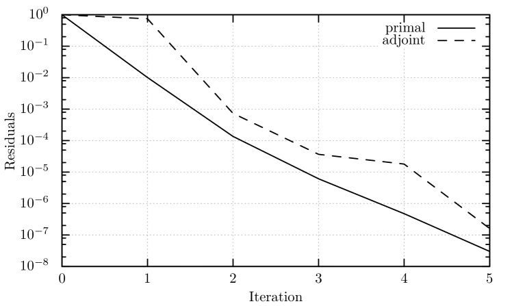
Figure 2: History of simultaneous piggyback iteration of primal and adjoint XBraid ($N=60000$).

The gradient provided by the adjoint XBraid solver is validated in Table 2 which shows good agreement with those computed from finite differences with a relative error below two percent.

Table 2: Validation of the gradient computed from the adjoint XBraid solver with finite differences.

	$\rho$	$\epsilon$	finite differences	adjoint sensitivity	rel. error
$N=60000$	$2$	$10^{-6}$	$0.231079186674421$	$0.230724810643109$	$0.15\%$
$N=60000$	$3$	$10^{-6}$	$0.224847819918494$	$0.223017099689057$	$0.81\%$
$N=60000$	$4$	$10^{-6}$	$0.200429607133401$	$0.196451436058937$	$1.98\%$
$N=120000$	$2$	$10^{-6}$	$0.231679529338891$	$0.232395575709547$	$0.31\%$
$N=120000$	$3$	$10^{-6}$	$0.225517896579319$	$0.225073911851428$	$0.19\%$
$N=120000$	$4$	$10^{-6}$	$0.199769404352068$	$0.198695760225926$	$0.54\%$
$N=240000$	$2$	$10^{-8}$	$0.232875008165934$	$0.234781281565824$	$0.81\%$
$N=240000$	$3$	$10^{-8}$	$0.227025065413500$	$0.228025754956746$	$0.44\%$
$N=240000$	$4$	$10^{-8}$	$0.201409511291217$	$0.204046297945359$	$1.31\%$

5.1 Parallel scaling for the primal and adjoint XBraid solver

A weak scaling study for the primal and the adjoint XBraid solver is shown in Table 3. The reported speedups are computed by dividing the runtime of the primal and adjoint XBraid solver by that of a classical time-serial primal forward and adjoint backward time stepper, respectively.

For these test cases, the runtimes of the adjoint XBraid solver show an overhead factor of about $12$ when compared to the corresponding runtimes of the primal one. However, a very similar factor of about $10$ can be observed for the time-serial computations. Thus, the observed overhead factor is mostly dominated by the adjoint time-stepping routine that computes $\left(\partial_{\vec{u}^{i-1},\rho}\Phi^{i}(\vec{u}^{i-1},\rho)\right)^{T}\vec{\bar{u}^{i}}$, which is needed in both the time-serial as well as the time-parallel computations. The additional overhead created by the AD-based derivation of the adjoint XBraid solver itself can therefore be estimated from $12/10=1.2$.

Table 3: Weak scaling study for the primal and adjoint XBraid solver.

			Primal
Number of	Number of		Iterations	Runtime	Runtime	Speedup
time steps	Cores		XBraid	XBraid	Serial
60000	64		5	0.49 sec	1.13 sec	2.84
120000	128		4	0.50 sec	2.97 sec	5.97
240000	256		4	0.76 sec	4.81 sec	6.31
			Adjoint
Number of	Number of		Iterations	Runtime	Runtime	Speedup
time steps	Cores		XBraid	XBraid	Serial
60000	64		6	6.54 sec	14.49 sec	2.22
120000	128		4	6.12 sec	26.27 sec	4.23
240000	256		4	9.44 sec	49.18 sec	5.21

Strong scaling results for primal as well as the adjoint runtimes are visualized in Figure 3, where the slope of reduction for the adjoint runtimes closely follows that of the primal one. This confirms that the adjoint XBraid solver indeed inherits the scaling behavior of the primal solver which is expected from its AD-based derivation. Since the primal XBraid solver is under active development, this property is particularly beneficial as improvements on primal scalability will automatically carry over to the adjoint code. The same data is used in Figure 4 to plot speedup when compared to a time-serial primal and adjoint time marching scheme. It shows the potential of the time-parallel adjoint for speeding up the runtime of existing unsteady adjoint time marching schemes for sensitivity evaluation.

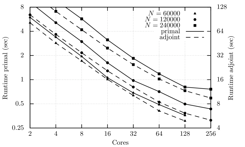
Figure 3: Strong scaling of primal (solid lines) and adjoint XBraid (dashed lines) solver for three different problem sizes.

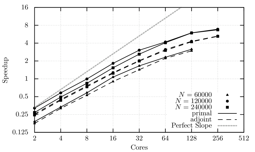
Figure 4: Speedup of primal and adjoint XBraid solver over serial forward and backward time stepping.

6 Conclusion

In this paper, we developed an adjoint solver that provides sensitivity computation for the parallel-in-time solver XBraid. XBraid applies nonlinear multigrid iterations to the time domain of unsteady partial differential equations and solves the resulting space-time system parallel-in-time. It operates through a high-level user interface that is non-intrusive to existing serial time marching schemes for solving unsteady PDEs. This property is of particular interest for applications where unsteady simulation tools have already been developed and refined over years, as is often the case for many CFD applications.

While the primal XBraid solver computes a space-time solution of the PDE for given input parameters and also evaluates objective functions that are of interest to the user, the proposed time-parallel adjoint XBraid solver computes derivatives of the objective function with respect to changes in the input parameters. Classical adjoint sensitivity computations for unsteady PDEs involve a forward-in-time sweep to compute the unsteady solution followed by a backwards-in-time loop to collect sensitivities. The parallel-in-time adjoint XBraid solver offers speedup by distributing the backwards-in-time phase onto multiple processors along the time domain. Its implementation is based on techniques of the reverse-mode of AD applied to one primal XBraid iteration. This yields a consistent discrete adjoint code that inherits parallel scaling properties from the primal solver and is non-intrusive to existing adjoint sequential time marching schemes.

The resulting adjoint solver adds two additional user routines to the primal XBraid interface: one for propagating sensitivities of the forward time stepper backwards in time and one for evaluating partial derivatives of the objective function at each time step. In cases where a time-serial unsteady adjoint solver is already available, this backwards time stepping capability can be easily wrapped into the adjoint XBraid interface with little extra coding.

The adjoint solver has been validated and tested on a model problem for advection-dominated flow. The original primal and adjoint time marching codes were limited to one processor such that a linear increase in the number of time steps results in a linear increase in corresponding runtime. This creates a situation analogous to the one where a spatially parallel code has reached its strong scaling limit. The parallel-in-time primal and adjoint XBraid solvers were able to achieve speedups of about $6$ (primal) and $5$ (adjoint) when compared to the serial ones, running on up to $256$ processors for the time parallelization. More importantly, the scaling behavior of the adjoint code in this test case is similar to that of the primal one such that improvements on the primal XBraid solver carry over to the adjoint implementation.

- (1) Albring, T., Dick, T., Gauger, N.R.: Assessment of the recursive projection method for the stabilization of discrete adjoint solvers. In: 18th AIAA/ISSMO Multidisciplinary Analysis and Optimization Conference, AIAA Aviation (2017)
- (2) Barker, A.T., Stoll, M.: Domain decomposition in time for pde-constrained optimization. Computer Physics Communications 197, 136–143 (2015)
- (3) Beyer, H.G., Sendhoff, B.: Robust optimization–a comprehensive survey. Computer methods in applied mechanics and engineering 196(33), 3190–3218 (2007)
- (4) Blazek, J.: Computational fluid dynamics: principles and applications, 2nd edn. Elsevier Ltd. (2005)
- (5) Bosse, T., Gauger, N.R., Griewank, A., Günther, S., Schulz, V.: One-shot approaches to design optimzation. In: G. Leugering, P. Benner, S. Engell, A. Griewank, H. Harbrecht, M. Hinze, R. Rannacher, S. Ulbrich (eds.) Trends in PDE Constrained Optimization, pp. 43–66. Springer International Publishing (2014)
- (6) Brandt, A.: Multi–level adaptive solutions to boundary–value problems. Math. Comp. 31(138), 333–390 (1977)
- (7) CoDiPack - Code Differentiation Package (Version 1.0). http://www.scicomp.uni-kl.de/software/codi/ (2017)
- (8) Du, X., Sarkis, M., Schaerer, C., Szyld: Inexact and truncated parareal-in-time krylov subspace methods for parabolic optimal control problems. ETNA 40, 36–57 (2013)
- (9) Economon, T., Palacios, F., Alonso, J.: Unsteady aerodynamic design on unstructured meshes with sliding interfaces. In: 51st AIAA Aerospace Sciences Meeting Including the New Horizons Forum and Aerospace Exposition, p. 632 (2013)
- (10) Emmett, M., Minion, M.: Toward an efficient parallel in time method for partial differential equations. Communications in Applied Mathematics and Computational Science 7(1), 105–132 (2012)
- (11) Falgout, R., Friedhoff, S., Kolev, T.V., MacLachlan, S., Schroder, J., Vandewalle, S.: Multigrid methods with space-time concurrency. SIAM J. Sci. Comput., submitted, LLNL-JRNL-678572 (2015)
- (12) Falgout, R.D., Friedhoff, S., Kolev, T.V., MacLachlan, S.P., Schroder, J.B.: Parallel time integration with multigrid. SIAM J. Sci. Comput. 36(6), C635–C661 (2014). LLNL-JRNL-645325
- (13) Falgout, R.D., Katz, A., Kolev, T.V., Schroder, J.B., Wissink, A., Yang, U.M.: Parallel time integration with multigrid reduction for a compressible fluid dynamics application. Tech. Rep. LLNL-JRNL-663416, Lawrence Livermore National Laboratory (2015)
- (14) Falgout, R.D., Manteuffel, T.A., O’Neill, B., Schroder, J.B.: Multigrid reduction in time for nonlinear parabolic problems. SIAM J. Sci. Comput. (to appear). LLNL-JRNL-692258
- (15) Farhat, C., Chandesris, M.: Time-decomposed parallel time-integrators: Theory and feasibility studies for uid, structure, and fluid–structure applications. Int. J. Numer. Meth. Engng 58, 1397–1434 (2003)
- (16) Ferziger, J., Peric, M.: Computational Methods for Fluid Dynamics, 3rd edn. Springer Berlin Heidelberg (2002)
- (17) Fischer, P., Hecht, F., Maday, Y.: A parareal in time semi-implicit approximation of the Navier-Stokes equations. In: Proceedings of the Fifteenth International Conference on Domain Decomposition Methods, pp. 433–440. Springer-Verlag (2005)
- (18) Gander, M.J.: 50 years of time parallel time integration. In: T. Carraro, M. Geiger, S. Körkel, R. Rannacher (eds.) Multiple Shooting and Time Domain Decomposition, pp. 69–114. Springer (2015)
- (19) Gander, M.J., Kwok, F.: Schwarz Methods for the Time-Parallel Solution of Parabolic Control Problems. In: Domain Decomposition Methods in Computational Science and Engineering XXII, Lecture Notes in Computational Science and Engineering, vol. 104, pp. 207–216. Springer-Verlag (2016)
- (20) Gander, M.J., Vandewalle, S.: Analysis of the parareal time-parallel time-integration method. SIAM J. Sci. Comput. 29(2), 556–578 (2007)
- (21) Gauger, N., Griewank, A., Hamdi, A., Kratzenstein, C., Özkaya, E., Slawig, T.: Automated extension of fixed point PDE solvers for optimal design with bounded retardation. In: G. Leugering, S. Engell, A. Griewank, M. Hinze, R. Rannacher, V. Schulz, M. Ulbrich, S. Ulbrich (eds.) Constrained Optimization and Optimal Control for Partial Differential Equations, pp. 99–122. Springer Basel (2012)
- (22) Giles, M., Pierce, N., Giles, M., Pierce, N.: Adjoint equations in CFD: Duality, boundary conditions and solution behaviour. In: 13th Computational Fluid Dynamics Conference, p. 1850 (1997)
- (23) Giles, M.B., Pierce, N.A.: An introduction to the adjoint approach to design. Flow, Turbulence and Combustion 65(3), 393–415 (2000)
- (24) Giles, M.B., Süli, E.: Adjoint methods for PDEs: a posteriori error analysis and postprocessing by duality. Acta numerica 11, 145–236 (2002)
- (25) Götschel, S., Minion, M.: Parallel-in-time for parabolic optimal control problems using pfasst. Tech. Rep. 17-51, ZIB (2017)
- (26) Griewank, A.: Projected hessians for preconditioning in one-step one-shot design optimization. In: G. Pillo, M. Roma (eds.) Large-Scale Nonlinear Optimization, pp. 151–171. Springer (2006)
- (27) Griewank, A., Faure, C.: Reduced functions, gradients and hessians from fixed-point iterations for state equations. Numer. Algorithms 30, 113–139 (2002)
- (28) Griewank, A., Ponomarenko, A.: Time-lag in derivative convergence for fixed point iterations. In: Proceedings of CARI’04, 7th African Conference on Research in Computer Science, pp. 295–304 (2004)
- (29) Griewank, A., Walther, A.: Evaluating Derivatives: Principles and Techniques of Algorithmic Differentiation. SIAM (2008)
- (30) Günther, S., Gauger, N.R., Wang, Q.: Simultaneous single-step one-shot optimization with unsteady pdes. Journal of Computational and Applied Mathematics 294, 12–22 (2016)
- (31) Heinkenschloss, M.: A time-domain decomposition iterative method for the solution of distributed linear quadratic optimal control problems. J. Comput. Appl. Math. 173(1), 169––198 (2005)
- (32) Jameson, A.: Aerodynamic design via control theory. Journal of Scientific Computing 3(3), 233–260 (1988)
- (33) Jameson, A.: Time dependent calculations using multigrid, with applications to unsteady flows past airfoils and wings. In: Proc. 10th Comp. Fluid Dyn. Conf., Honolulu, USA, June 24-26, AIAA-Paper 91-1596 (1991)
- (34) Josuttis, N.M.: The C++ standard library: a tutorial and reference. Addison-Wesley (2012)
- (35) Kanamaru, T.: Van der pol oscillator. Scholarpedia 2(1), 2202 (2007)
- (36) Krause, R., Ruprecht, D.: Hybrid space–time parallel solution of Burgers’ equation. In: Domain Decomposition Methods in Science and Engineering XXI, pp. 647–655. Springer (2014)
- (37) Kwok, F.: On the time-domain decomposition of parabolic optimal control problems. In: Domain Decomposition Methods in Science and Engineering XXIII, pp. 55–67. Springer (2017)
- (38) Lions, J.L.: Optimal control of systems governed by partial differential equations problèmes aux limites (1971)
- (39) Lions, J.L., Maday, Y., Turinici, G.: Résolution d’EDP par un schéma en temps pararéel. C.R.Acad Sci. Paris Sér. I Math 332, 661–668 (2001)
- (40) Mathew, T.P., Sarkis, M., Schaerer, C.E.: Analysis of block parareal preconditioners for parabolic optimal control problems. SIAM Journal on Scientific Computing 32(3), 1180–1200 (2010)
- (41) Mavriplis, D.: Solution of the unsteady discrete adjoint for three-dimensional problems on dynamically deforming unstructured meshes. In: 46th AIAA Aerospace Sciences Meeting and Exhibit, p. 727 (2008)
- (42) Mohammadi, B., Pironneau, O.: Applied shape optimization for fluids. Oxford University Press (2010)
- (43) Nadarajah, S.K., Jameson, A.: Optimum shape design for unsteady flows with time-accurate continuous and discrete adjoint method. AIAA journal 45(7), 1478–1491 (2007)
- (44) Naumann, U.: The Art of Differentiating Computer Programs: An Introduction to Algorithmic Differentiation. Software, Environments, and Tools. Society for Industrial and Applied Mathematics (2012)
- (45) Navon, I.: Practical and theoretical aspects of adjoint parameter estimation and identifiability in meteorology and oceanography. Dynamics of Atmospheres and Oceans 27(1), 55 – 79 (1998)
- (46) Nielsen, E.J., Diskin, B., Yamaleev, N.K.: Discrete adjoint-based design optimization of unsteady turbulent flows on dynamic unstructured grids. AIAA journal 48(6), 1195–1206 (2010)
- (47) Nievergelt, J.: Parallel methods for integrating ordinary differential equations. Comm. ACM 7, 731–733 (1964)
- (48) Pierce, N.A., Giles, M.B.: Adjoint recovery of superconvergent functionals from PDE approximations. SIAM review 42(2), 247–264 (2000)
- (49) Pironneau, O.: On optimum design in fluid mechanics. Journal of Fluid Mechanics 64(1), 97–110 (1974)
- (50) Ries, M., Trottenberg, U.: MGR-ein blitzschneller elliptischer löser. Tech. Rep. Preprint 277 SFB 72, Universität Bonn (1979)
- (51) Ries, M., Trottenberg, U., Winter, G.: A note on MGR methods. Linear Algebra Appl. 49, 1–26 (1983)
- (52) Rumpfkeil, M., Zingg, D.: A general framework for the optimal control of unsteady flows with applications. In: 45th AIAA Aerospace Sciences Meeting and Exhibit, p. 1128 (2007)
- (53) Ruprecht, D., Krause, R.: Explicit parallel-in-time integration of a linear acoustic-advection system. Computers & Fluids 59, 72–83 (2012)
- (54) Shroff, G.M., Keller, H.B.: Stabilization of unstable procedures: the recursive projection method. SIAM Journal on numerical analysis 30(4), 1099–1120 (1993)
- (55) Steiner, J., Ruprecht, D., Speck, R., Krause, R.: Convergence of parareal for the Navier-Stokes equations depending on the Reynolds number. In: A. Abdulle, S. Deparis, D. Kressner, F. Nobile, M. Picasso (eds.) Numerical Mathematics and Advanced Applications - ENUMATH 2013: Proceedings of ENUMATH 2013, the 10th European Conference on Numerical Mathematics and Advanced Applications, Lausanne, August 2013, pp. 195–202. Springer International Publishing, Cham (2015)
- (56) Trottenberg, U., Oosterlee, C., Schüller, A.: Multigrid. Academic Press, San Diego (2001)
- (57) Tucker, P.: Unsteady computational fluid dynamics in aeronautics. Springer Science & Business Media (2014)
- (58) V. Dobrev Tz. Kolev, N.P., Schroder, J.: Two-level convergence theory for multigrid reduction in time (MGRIT). Copper Mountain Special Section, SIAM J. Sci. Comput. (submitted) (2016). LLNL-JRNL-692418
- (59) Venditti, D.A., Darmofal, D.L.: Grid adaptation for functional outputs: application to two-dimensional inviscid flows. Journal of Computational Physics 176(1), 40–69 (2002)
- (60) XBraid: Parallel multigrid in time. http://llnl.gov/casc/xbraid