Vertex Nomination via Seeded Graph Matching

Abstract

[Summary] Consider two networks on overlapping, non-identical vertex sets. Given vertices of interest in the first network, we seek to identify the corresponding vertices, if any exist, in the second network. While in moderately sized networks graph matching methods can be applied directly to recover the missing correspondences, herein we present a principled methodology appropriate for situations in which the networks are too large/noisy for brute-force graph matching. Our methodology identifies vertices in a local neighborhood of the vertices of interest in the first network that have verifiable corresponding vertices in the second network. Leveraging these known correspondences, referred to as seeds, we match the induced subgraphs in each network generated by the neighborhoods of these verified seeds, and rank the vertices of the second network in terms of the most likely matches to the original vertices of interest. We demonstrate the applicability of our methodology through simulations and real data examples.

, , , and (2019), Vertex Nomination via Seeded Graph Matching, Statistical Analysis and Data Science

1 Introduction and Background

In this paper, we address the problem of nominating vertices across a pair of networks: Given vertices of interest (VOIs) in a network $G=(V,E)$, our task is to identify the corresponding vertices of interest, if they exist, in a second network $G^{\prime}=(V^{\prime},E^{\prime})$. Our methods will leverage vertices in the neighborhood of the VOIs in $G$ that have verifiable matches in $G^{\prime}$ to (ideally) create local neighborhoods of the VOIs in both $G$ and $G^{\prime}$. These neighborhoods are then soft-matched (see Algorithm 1, adapted here from ¹¹) across networks, yielding a nomination list for each VOI in $G$; i.e., a ranking of the vertices in the local neighborhood of the seeds in $G^{\prime}$, ideally with the corresponding VOI’s in $G^{\prime}$ concentrating at the top of the list. While global methods can (and have been) applied to identify the VOI’s in $G^{\prime}$ directly, performance of these methods can suffer from the noise induced by vertices without correspondences across networks ²⁸. Localization is a prominent tool used across various fields such as machine learning (see for example ^{41, 53} on using locality based anomaly detection in time series of graphs and ¹⁶ on localized multiple kernel learning), pattern recognition (this includes clustering algorithms which have been using localization for many years — for example $k$-nearest neighbor based classification rules — see for example ^{47, 15, 23, 37, 8}), and object recognition (see for example ⁴⁶ on using convolutional networks for localization and object boundary detection and ⁴ on local algorithms for geometric object recognition). Inspired by the many successes localization has seen in other fields of research, we bring the concept of localization to the fore-front of network alignment. Our methods are inherently local, leveraging recent advancements in both graph matching ^{11, 29} and vertex nomination ^{7, 12} to nominate across essentially arbitrarily large networks.

Formally, suppose we are given two networks $G=(V,E)$ and $G^{\prime}=(V^{\prime},E^{\prime})$ on overlapping but not necessarily identical vertex sets $V$ and $V^{\prime}$ respectively. For simplicity, we will presently restrict our attention to the case of a single VOI in $G$ (as the case of multiple VOIs is an immediate extension of our methodology for a single VOI), and we write

$$V=\{x\}\cup S\cup W\cup J,\,\,\,\,\,\,V^{\prime}=\{x^{\prime}\}\cup S^{\prime}\cup W^{\prime}\cup J^{\prime},$$

where $x$ and $x^{\prime}$ represent the VOI in $G$ and $G^{\prime}$ resp.; $S$ and $S^{\prime}$ represent the seeded vertices across networks—those vertices that appear in both vertex sets whose correspondence across networks (i.e., the seeding $S\leftrightarrow S^{\prime}$) is known a priori—and necessarily satisfy $s:=|S|=|S^{\prime}|$; $W$ and $W^{\prime}$ are the shared non-seed vertices—those vertices that appear in both vertex sets whose correspondence across networks is unknown a priori—with $|W|=|W^{\prime}|=n$; and $J$ and $J^{\prime}$ are the unshared vertices—those vertices that appear in only one or the other vertex set without correspondences across networks—with $|J|=m$ and $|J^{\prime}|=m^{\prime}$. Thus, we can write

$$\eta:=|V|=1+s+n+m,\,\,\,\text{ and }\eta^{\prime}=|V^{\prime}|=1+s+n+m^{\prime}.$$

While the correspondence between vertices in $W$ and $W^{\prime}$ is unknown a priori, we will further assume that it is unknown which vertices in $G\setminus\{x,S\}$ are in $W$ versus $J$, as are the values of $n,m$ and $m^{\prime}$. Our inference task is to identify $x^{\prime}\in V^{\prime}\setminus S^{\prime}$ (i.e., the corresponding VOI in $G^{\prime}$) using only the knowledge of the graph structures and the correspondence $S\leftrightarrow S^{\prime}$. For the purposes of this paper, we will assume that the corresponding vertex $x^{\prime}$ does exist in $G^{\prime}$, else our task is impossible. Our goal will be to nominate vertices in $G^{\prime}$ in a principled manner so that the true match is high in the nomination list, thus saving the end-user time in searching for this true match. While this core-junk network framework has appeared often in the literature (see, for example, ²²), herein we will consider a more general random graph model that allows for heterogeneity in vertex degree and behavior (see, Section 3).

Our approach to this inference task lies on the boundary between Graph Matching and Vertex Nomination. Stated simply, the formulation of the graph matching problem (GMP) considered herein seeks to align the vertices in two networks so as to minimize the number of induced edge disagreements between the aligned networks. Graph matching has been been extensively studied in the literature (for an excellent survey of the literature, see ^{5, 13}) with applications across various fields including pattern recognition (see, for example, ^{2, 54, 60}), computer vision (see, for example, ^{59, 26, 55}), and biology (see, for example, ^{57, 36, 24}), among others. The seeded graph matching SGM algorithm on which we base our primary algorithm has run-time $O(n^{3})$ at worst, which has been shown to be reasonable in comparison to other state-of-the-art algorithms (such as the PATH algorithm of ⁵⁸ – see ⁵² and ¹¹ for more information on the computational complexity of this algorithm). Furthermore, the authors of ^{30, 29} show that it has theoretical guarantees for converging to the correct solution under reasonable model assumptions.

The classical formulation of the vertex nomination (VN) inference task ^{34, 6, 48, 50, 12, 31} can be stated as follows: given a network with latent community structure in which one of the communities is of particular interest and given a few vertices from the community of interest, the task in vertex nomination is to order the remaining vertices in the network into a nomination list, with the aim of having vertices from the community of interest concentrate at the top of the list. Thus, vertex nomination can also be thought of as a method for inferring missing vertex labels, and is related to the class/labeled instances acquisition task and collective classification methods of ^{3, 51, 45}. The goal of vertex nomination is similar in spirit to popular network-based information retrieval (IR) procedures such as PageRank ³⁹ and personalized recommender systems on graphs ¹⁹. However, this formulation of VN is distinguished from other supervised network mining tasks in both the generality of what defines a vertex of interest ^{43, 32} and the (often) limited nature of the available training data (i.e., known vertices of interest) in $G$. Our present task can be viewed as vertex nomination across networks: for a vertex of interest in $G$, we use graph matching methodologies to order the vertices in $G^{\prime}$ into a nomination list, with the aim of having the corresponding vertex of interest in $G^{\prime}$ near the top of the list.

Our contributions:

In summary, our contributions are as follows:

• Leveraging the idea of principled sub-sampling of a graph, we reduce time-complexity for matching two graphs via localization.

• Combining the task of vertex nomination to across graph nomination tasks.

• Extending the SoftSGM algorithm of ¹¹ to the task of vertex nomination.

• Demonstrating via two real world graph data-sets, we conduct an out-of-the-box large-scale evaluation of our VNmatch algorithm.

The remainder of the paper is laid out as follows: In Section 2, we give an overview of some related work, after which, in Section 3, we introduce a formal definition of what we mean by "corresponding vertices." Following, in Section 4, we introduce our across graph VN scheme, VNmatch, along with a brief mathematical description of the utilized subroutines including the soft seeded graph matching algorithm (SoftSGM, Algorithm 1), introduced in ¹¹. In Sections 5.1 and 5.2, we explore applications of VNmatch on both synthetic and real data, including a pair of high school friendship networks and a pair of online social networks. We conclude with an overview of our findings and a discussion of potential extensions in Section 6.

We employ the SoftSGM Algorithm of ¹¹ as a means by which to nominate vertices in the VNmatch algorithm so as to introduce this algorithm as a useful tool in the across graph vertex nomination task. However, other vertex nomination schemes exist which could also be adapted and utilized in the VNmatch algorithm (in particular Steps 3 and 4). For example, the use of spectral methods, which tend to work well for matching larger graphs, may be desirable when the original graphs are on the order of millions of vertices and localization trims the networks down to only thousands of vertices. For details regarding adjacency or Laplacian spectral embedding, see ⁴².

Notation:

To aid the reader, we have collected the frequently used notation introduced in this manuscript into a table for ease of reference; see Table 1. Also, in what follows, we assume for simplicity that all graphs are simple (that is, edges are undirected, there are no multi-edges, and there are no loops).

Table 1: Table of frequently used notation

Symbol	Description
$G=(V,E)$	A graph with vertex set, $V$, and edge set, $E$
$G[T]$	For $T\subset V$, this is the induced subgraph of $G$ on $T$
$\eta$ (resp., $\eta^{\prime}$)	Number of vertices in $V$ (resp., $V^{\prime}$)
$S$ (resp., $S^{\prime}$)	Set of $s$ seed vertices in $G$ (resp., $G^{\prime})$
$x$ (resp., $x^{\prime}$)	Vertex of interest in $G$ (resp., $G^{\prime}$)
$W$ (resp., $W^{\prime}$)	Set of all $n$ shared non-seed and non-VOI vertices in $G$ (resp., $G^{\prime}$)
$U$ (resp., $U^{\prime}$)	Set of all shared vertices, including seeds and VOI in $G$ (resp., $G^{\prime}$)
$J$ (resp., $J^{\prime}$)	Set of $m$ (resp., $m^{\prime}$) unshared vertices in $G$ (resp., $G^{\prime}$)
$H$ (resp., $H^{\prime}$)	$G[U]$ (resp., $G^{\prime}[U^{\prime}]$)
$N_{t}(T)$,	Set of all vertices within $t$-length path of $T\subset V$ (including $T$)
$I_{n}(0_{n})$	The $n\times n$ identity (zeroes) matrix
$\mathbb{1}$	Appropriately sized vector of all ones
$\Pi_{k}$	Set of all $k\times k$ permutation matrices
$\mathcal{D}_{k}$	Set of all $k\times k$ doubly stochastic matrices
$h$	Maximum considered path length from seeds to VOI, $x\in G$
$S_{x}$ and $S_{x}^{\prime}$	$S_{x}=S\cap N_{h}(x)$ with corresponding seeds $S_{x}^{\prime}$ in $V^{\prime}$
$\ell$	Maximum path length for neighborhood around $S_{x}$
$G_{x}=(V_{x},E_{x})$ (resp., $G_{x}^{\prime}=(V_{x}^{\prime},E_{x}^{\prime})$)	$G[N_{\ell}(S_{x})]$ (resp., $G^{\prime}[N_{\ell}(S_{x}^{\prime})]$)
$C_{x}^{\prime}$	The set of candidate matches for $x$ in $V_{x}^{\prime}$, namely $C_{x}^{\prime}=V_{x}^{\prime}\setminus S_{x}^{\prime}$
$\Phi_{x}$	Nomination list output from Algorithm 2
$\tau(x^{\prime})$	Normalized expected location of $x^{\prime}$ in $\Phi_{x}$
$|T|$	Cardinality of set $T$
$\left\|A\right\|_{F}$	Frobenius norm of matrix $A$
$\oplus$	direct sum

2 Related Work

A number of inexact graph matching algorithms have been extended/developed recently to match graphs with overlapping, non-identical vertex sets. Two such algorithms include percolation based algorithms (see for example ^{22, 9, 21}) and Bayesian based algorithms (see for example ⁴⁰).

In ²² and ²¹, the authors focus their efforts on proving that under the independent-edge-sampling model $G(n,p;t.s)$, where a graph, $G$, is generated from an Erdös-Renyi $(n,p)$ model and two subgraphs of $G$, namely $G_{1}$ and $G_{2}$, are generated so that the probability of a node from $G$ belonging to $G_{i}$ is $s$, independently for $i=1,2$, and similarly for edges (with probability $t$). Under the independent-edge-sampling model, it is shown in ²² that for sufficiently large $p$ the true partial matching is recoverable under particular model assumptions and for some formulation of their objective; however, as the authors admit, the optimization formulation proposed is not scalable, and there is no mention of how the correct formulation of the objective is to be obtained.

Using the same independent-edge-sampling model, the authors of ²¹ introduce an iterative percolation based graph matching method for seed-based graph matching, demonstrating that their method (under this model and particular assumptions) matches nearly all overlapping nodes correctly. In ⁹, the authors introduce a degree-driven percolation based graph matching algorithm which uses an iterative approach to match nodes with higher degree to lower degree using percolation based graph matching. For scale-free networks, the authors show that, under particular model assumptions, their method, which does not aim to match all nodes, but to match subsets of nodes from the two graphs, matches nearly all vertices which have a match correctly and that the algorithm does not match any nodes incorrectly. While this works well for scale-free networks, the advantages of this method would be more limited on graphs with more block structure and without having higher-degree nodes which help seed the rest of the algorithm. The authors point out that when seeds are chosen uniformly at random $o(n^{1/2+\epsilon})$ seeds are needed to match most vertices correctly, but allowing for more intelligent seed-selection based on vertex degree, as few as $n^{\epsilon}$ seeds may be sufficient, for some arbitrarily small $\epsilon$.

Each of the above approaches is theoretically based in relatively simple random graph models (ER for ²² and the Chung-Lu model in ⁹), while also demonstrating good performance in more complex real data settings. Our present approach is naturally situated in the more general Random Dot Product Graph setting of ⁵⁶. While still not able to capture all the intricacies of real network data, the random dot product graph is quite flexible and encompasses numerous other common random graph models (ER, Chung-Lu, positive definite stochastic blockmodel, etc.). In addition, we also demonstrate the effectiveness of our method on more complex real data networks as well.

Percolation based algorithms could certainly be used for vertex nomination in a similar way that we present vertex nomination based on the seeded graph matching algorithm of ¹¹ (which is based on a fast approximate quadratic programming algorithm of ⁵²). One of the advantages of the present optimization based approach is the ability to efficiently explore the space of locally optimal solutions near the global optimum. Practically, the graphs to be matched in real data are much more messy than theory would allow, and the variations that can be obtained from these local optima provide a degree of robustness to model misspecification. Furthermore, the SGM algorithm itself runs quickly on modestly sized networks and has asymptotic guarantees for particular models and conditions (see for example ^{52, 11} and ^{30, 29}).

In ²⁰ the authors focus on the task of de-anonymizability, and explore a method for matching nodes based on node-degree; that is, the authors consider two graphs drawn in some manner from a larger graph and attempt to de-anonymize (match) the vertices in the two graphs which have the highest degrees. We are not concerned with matching vertices based on their degree, since a vertex of interest is based on an external characteristic that is not necessarily related to the degree distribution of the two graphs.

Another technique for approximate graph matching relies on Bayesian methods ⁴⁰. The authors of ⁴⁰ introduce a method which relies on estimating the posterior probability that two nodes should be matched based on a particular prior. In the afore-mentioned paper, the authors rely on node attributes, such as vertex degree, mapping a few nodes at a time in an iterative manner until all nodes are matched; any nodes matched in one iteration will be used as seeds (referred to as anchors) in the next iteration. In the end, the authors seek to obtain a hard matching of the nodes that maximizes the sum of the log-posteriors for all node pairs. While the idea of a posterior probability that two nodes should be matched is a similar idea to what we present, the purpose of our more frequentist method is to utilize a soft matching of the nodes in order to rank them in order from most to least likely matches to the vertex (or vertices) of interest.

3 Corresponding vertices

Consider two social networks in which vertices represent users/accounts and edges represent whether or not two accounts are linked in some way. An individual may have an account on one network or the other or both. We would say that two accounts across the platforms correspond to each other if the same individual runs both accounts; that is, both nodes correspond to the same individual although with possibly different node labels. Arguably an individual who has an account on both networks will have similar, though not identical, behavior across the two networks. Consider an email network in which nodes are email addresses and two email addresses share an edge (directed or not) if they send correspondence to one another, and a phone network in which nodes are phone numbers and edges represent whether or not one of the numbers calls the other. In this example, a vertex in the email network will correspond to a vertex in the call network if the email and phone number belong to the same individual. An individual who uses both email and phone correspondence may communicate with individuals in the two networks in a similar, though not identical, manner. Thus, if there is a connection between two individuals in one network and those same individuals exist in the second network, one would think that it is more likely that there exists a connection between these individuals in the second network, i.e. there is a positive correlation between the edges between these vertices across the networks. To model this correspondence, we proceed as follows.

With notation as above, let $U=\{x\}\cup S\cup W$ and $U^{\prime}=\{x^{\prime}\}\cup S^{\prime}\cup W^{\prime}$ denote the set of shared vertices between $G$ and $G^{\prime}$ with $|U|=|U^{\prime}|=1+s+n$. Define $H:=G[U]$ (resp., $H^{\prime}=G^{\prime}[U^{\prime}]$), the induced subgraph of $G$ (resp., $G^{\prime}$) on the vertex set $U$ (resp., $U^{\prime}$). As $H$ and $H^{\prime}$ are graphs on the same (though potentially differently labeled) vertex sets, we model a shared structure present across $H$ and $H^{\prime}$ as $(H,H^{\prime})\sim\rho\hbox{\sout{ }}RDPG(X)$. Before defining the $\rho\hbox{\sout{ }}RDPG$ model, we first recall the definition of a random dot product graph (RDPG); see ⁵⁶.

Definition 3.1.

Consider $X=[X_{1},\ldots,X_{n}]^{\top}\in\mathbb{R}^{n\times d}$ satisfying $XX^{\top}\in[0,1]^{n\times n}$. We say that graph $G$ with adjacency matrix $A$ is distributed as a random dot product graph with parameter $X$ (abbreviated $G\sim RDPG(X)$) if given $X$,

$$A_{i,j}\stackrel{{\scriptstyle\text{ind.}}}{{\sim}}Bernoulli(X_{i}^{\top}X_{j}),$$

i.e.,

$$P(A|X)=\prod_{i<j}(X_{i}^{\top}X_{j})^{A_{i,j}}(1-X_{i}^{\top}X_{j})^{1-A_{i,j}}.$$

Conditioning on $X$, this is an independent-edge random graph model where vertex $v_{i}$ is associated with a latent position vector $X_{i}\in\mathbb{R}^{d}$, and the probability of an edge between any two vertices is determined by the dot product of their associated latent position vectors.

To imbue multiple random dot product graphs with a notion of vertex correspondence, we correlate the behavior of nodes across networks. We call this new model the $\rho\hbox{\sout{ }}RDPG$ model, which is defined as follows.

Definition 3.2.

Consider $X=[X_{1},\ldots,X_{n}]^{\top}\in\mathbb{R}^{n\times d}$ satisfying $XX^{\top}\in[0,1]^{n\times n}$. The bivariate graph valued random variables $(G,G^{\prime})$—with respective adjacency matrices $A$ and $A^{\prime}$—are said to be distributed as a pair of $\rho$-correlated random dot product graphs with parameter $X$ (abbreviated $(G,G^{\prime})\sim\rho\hbox{\sout{ }}RDPG(X)$) if

1. Marginally, $G,G^{\prime}\sim RDPG(X)$, and

2. $\{A_{i,j},A^{\prime}_{k,l}\}_{\{i,j\},\{k,l\}\in\binom{V}{2}}$ are collectively independent except that for each $\{i,j\}\in\binom{V}{2}$, $\mathrm{correlation}(A_{i,j},A^{\prime}_{i,j})=\rho.$

Our framework posits $(H,H^{\prime})\sim\rho\hbox{\sout{ }}RDPG(X)$ for a latent position matrix $X\in\mathbb{R}^{(1+s+n)\times d}$. In order to generate the full graphs $G$ and $G^{\prime}$ which also have unshared vertices, we generate $G\sim RDPG([X,Y])$ and $G^{\prime}\sim RDPG([X,Y^{\prime}])$, so that the induced subgraphs $(H,H^{\prime})\sim\rho\hbox{\sout{ }}RDPG(X)$ and the remaining edges of $G$ and $G^{\prime}$ are formed independently as in the case for the general RDPG. Thus, the first $1+s+n$ vertices in the two graphs correspond to one another via the identity map and the remaining $m$ and $m^{\prime}$ vertices of $G$ and $G^{\prime}$, respectively, represent the unshared vertices $J$ and $J^{\prime}$. Here, $Y\in\mathbb{R}^{m\times d}$ and $Y^{\prime}\in\mathbb{R}^{m^{\prime}\times d}$ represent the respective latent positions for the unshared vertices in $G$ and $G^{\prime}$. For ease of notation, we will write $(G,G^{\prime})\sim\rho\hbox{\sout{ }}RDPG(X,Y,Y^{\prime})$, where $(G,G^{\prime})$ is realized as two graphs: $G$ on $\eta=1+s+n+m$ vertices $\{x\}\cup S\cup W\cup J$ and $G^{\prime}$ on $\eta^{\prime}=1+s+n+m^{\prime}$ vertices $\{x^{\prime}\}\cup S^{\prime}\cup W^{\prime}\cup J^{\prime}$.

If $G$ and $G^{\prime}$ exhibit latent community structure, it can be fruitful to model them as Stochastic block model (SBM) random graphs ¹⁸. SBMs have been extensively studied in the literature and have been shown to provide a useful and theoretically tractable model for more complex graphs with underlying community structure ^{44, 49, 1, 38}. We define the stochastic block model as follows.

Definition 3.3.

We say that graph $G=(V,E)$ with adjacency matrix $A$ is distributed as a stochastic block model random graph with parameters $k$, $b$ and $\Lambda$ (abbreviated $G\sim\text{SBM}(k,b,\Lambda)$) if

1. $V$ is partitioned into $k$ blocks $V=V_{1}\cup V_{2}\cup\cdots\cup V_{k}$;

2. $b:V\to\{1,\ldots,k\}$ is a map such that $b(i)$ denotes the block label of the $i^{\text{th}}$ vertex;

3. $\Lambda\in[0,1]^{k\times k}$ is a matrix such that $A_{i,j}\stackrel{{\scriptstyle ind}}{{\sim}}$Bernoulli$(\Lambda_{b(i),b(j)})$ for distinct $\{i,j\}\in\binom{V}{2}$.

Recall that the edge probability matrix for a random dot product graph model, with parameter $X\in\mathbb{R}^{n\times d}$, is equal to $XX^{T}$, which is positive semi-definite. If $X$ consists of precisely $k$ distinct rows, then a graph generated via $RDPG(X)$ can also be said to be generated from a stochastic block model having $k$ blocks, block assignment vector $b$ assigning vertices with the same latent position to the same block, and probability matrix $\Lambda=X^{(k)}(X^{(k)})^{T}$ where $X^{(k)}$ here refers to the $k\times d$ matrix of distinct rows of $X$. Moreover, if $\Lambda$ is positive semidefinite, then $G\sim\text{SBM}(k,b,\Lambda)$ can be realized as a RDPG with appropriately defined $X$. Thus, there is an overlap in the set of random dot product graph models and stochastic block models.

We can then define the $\rho\hbox{\sout{ }}SBM$ model as follows.

Definition 3.4.

The bivariate graph valued random variables $(G,G^{\prime})$—with respective adjacency matrices $A$ and $A^{\prime}$—are said to be distributed as a pair of $\rho$-correlated stochastic block model graphs with parameter $k$, $b$, and $\Lambda$ (abbreviated $(G,G^{\prime})\sim\rho\hbox{\sout{ }}\text{SBM}(k,b,\Lambda)$) if

1. Marginally, $G,G^{\prime}\sim\text{SBM}(k,b,\Lambda)$, and

2. $\{A_{i,j},A^{\prime}_{k,l}\}_{\{i,j\},\{k,l\}\in\binom{V}{2}}$ are collectively independent except that for each $\{i,j\}\in\binom{V}{2}$,

   $$\text{correlation}(A_{i,j},A^{\prime}_{i,j})=\rho.$$

Note that if we generate $H$ and $H^{\prime}$ from a $\rho\hbox{\sout{ }}SBM(k,b,\Lambda)$, $G$ and $G^{\prime}$ can be constructed so that

$$G\sim\rho\hbox{\sout{ }}SBM(k_{1},b_{1},\Lambda_{1})\text{ and }G^{\prime}\sim\rho\hbox{\sout{ }}SBM(k_{2},b_{2},\Lambda_{2}),$$

where $k\leq\min(k_{1},k_{2}),$ $b_{1}(j)=b_{2}(j)=b(j)$ for all $j\in\{1,2,\ldots,1+s+n\}$, and the upper left $k\times k$ submatrix of $\Lambda_{i}$ is $\Lambda$ (for $i=1,2$). We write this formally as

$$(G,G^{\prime})\sim\rho\hbox{\sout{ }}SBM(k_{1},k_{2},b_{1},b_{2},\Lambda_{1},\Lambda_{2}).$$

4 Vertex nomination via seeded graph matching

With this notion of corresponding vertices, we next introduce our proposed algorithm for finding the corresponding vertex $x^{\prime}\in V^{\prime}$ to a particular vertex of interest $x\in V$. Again, we assume a single vertex of interest for simplicity, as the extension to multiple vertices of interest follows immediately. Before presenting our main algorithm, VNmatch (Algorithm 2), we first provide the necessary details for the subroutine of Algorithm 2 we employ, namely the SoftSGM algorithm of ¹¹. The easy interpretability and simple extension of the SoftSGM algorithm to generating nomination lists for vertices of interest make it a natural candidate for the vertex nomination subroutine task of Algorithm 2; however, other methods of graph matching, such as spectral-based methods, for which extension to vertex nomination is possible could also be used during this step of the algorithm.

4.1 Soft seeded graph matching

Given $A$ and $A^{\prime}$ in $\mathbb{R}^{n\times n}$, the respective adjacency matrices of two $n$-vertex graphs $G$ and $G^{\prime}$, the graph matching problem (GMP) is

$$\min_{P\in\Pi_{n}}\|AP-PA^{\prime}\|_{F},$$ (1)

where $\Pi_{n}$ is the set of $n\times n$ permutation matrices, and $\left\|M\right\|_{F}$ denotes the Frobenius norm of the matrix $M$. While the formulation in Eq. (1) seems restrictive, it is easily adapted to handle the case where the graphs are weighted, directed, loopy and on potentially different sized vertex sets (using, for example, the padding methods introduced in ¹¹).

In our present setting, where we have known seeded vertices $S\leftrightarrow S^{\prime}$, we consider the closely related seeded graph matching problem (SGMP) (see, for example, ^{11, 30, 29, 17, 13, 28, 33}). We have $G=(V,E)$ and $G^{\prime}=(V^{\prime},E^{\prime})$ with vertex sets $V=\{x\}\cup S\cup W\cup J$ and $V^{\prime}=\{x^{\prime}\}\cup S^{\prime}\cup W^{\prime}\cup J^{\prime}$, with $|V|=\eta=1+s+n+m$, $|V^{\prime}|=\eta^{\prime}=1+s+n+m^{\prime}$, and seeding $S\leftrightarrow S^{\prime}$. Without loss of generality, suppose $S=S^{\prime}=\{1,2,\ldots,s\}$ (if no seeds are used, $s=0$ and $S=S^{\prime}=\emptyset$), and suppose for the moment that $\eta=\eta^{\prime}$. The seeded graph matching problem aims to solve

$$\min_{P\in\Pi_{\eta-s}}\left\|A(I_{s}\oplus P)-(I_{s}\oplus P)A^{\prime}\right\|_{F}^{2},$$ (2)

where, $\Pi_{\eta-s}$ denotes the set of $(\eta-s)\times(\eta-s)$ permutation matrices, and $\oplus$ denotes the direct sum of matrices. Note that decomposing $A$ and $A^{\prime}$ via

$$A=\begin{pmatrix}A_{11}&A_{12}\\ A_{21}&A_{22}\end{pmatrix},\text{ and }A^{\prime}=\begin{pmatrix}A^{\prime}_{11}&A^{\prime}_{12}\\ A^{\prime}_{21}&A^{\prime}_{22}\end{pmatrix}$$ (3)

where $A_{11},\,A^{\prime}_{11}\in\mathbb{R}^{s\times s}$, $A_{21}^{T},\,(A^{\prime}_{21})^{T},A_{12},\,A^{\prime}_{12}\in\mathbb{R}^{(\eta-s)\times s}$, and $A_{22},\,A^{\prime}_{22}\in\mathbb{R}^{(\eta-s)\times(\eta-s)}$, the SGMP is equivalent to

$$\max_{P\in\Pi_{\eta-s}}f(P)=\max_{P\in\Pi_{\eta-s}}\left[\textup{trace}(P^{T}A_{21}(A^{\prime}_{21})^{T})+\right.\\ \left.\textup{trace}(P^{T}A^{T}_{12}A^{\prime}_{12})+\textup{trace}(A_{22}^{T}PA^{\prime}_{22}P^{T})\right].$$ (4)

The SGMP, in general, is NP-hard, and many (seeded) graph matching algorithms begin by relaxing the feasible region of Eq. (2) or (4) from the discrete $\Pi_{\eta-s}$ to the convex hull of $\Pi_{\eta-s}$ ^{58, 10, 52, 11}, which, by the Birkoff-vonNeumann theorem, is the set of $(\eta-s)\times(\eta-s)$ doubly stochastic matrices, denoted $\mathcal{D}_{\eta-s}$. This relaxation enables the machinery of continuous optimization (gradient descent, ADMM, etc.) to be employed on the relaxed SGMP. Note that while the solutions of Eq. (2) and (4) are equivalent, the solutions of the relaxations of Eq. (2) and (4) are not equivalent in general, with the indefinite relaxation, Eq. (4), preferable under the model assumptions we will consider in this paper ²⁹.

The SGM algorithm of ¹¹ approximately solves this indefinite SGMP relaxation using the Frank-Wolfe algorithm ¹⁴, and then projects the obtained doubly stochastic solution onto $\Pi_{\eta-s}$. The algorithm performs excellently in practice in both synthetic and real data settings, with a $O((\eta-s)^{3})$ runtime allowing for its efficient implementation on modestly sized networks. Since we ultimately aim to create a nomination list (and not a 1–to–1 correspondence necessarily) for the VOI of likely matches in $V^{\prime}\backslash S^{\prime}$, we use the SoftSGM algorithm of ¹¹—a stochastic averaging of the original SGM procedure over multiple random restarts—in order to softly match the graphs. Rather than the 1–to–1 correspondence output from SGM, SoftSGM (pseudocode provided in Algorithm 1 for completeness) outputs a function $p(\cdot,\cdot):V\times V^{\prime}\mapsto[0,1]$, where $p(i,j)$ represents the likelihood vertex $j$ in $G^{\prime}$ matches to vertex $i$ in $G$. As noted in Table 1, $A\oplus B$ denotes the direct sum between two matrices $A$ and $B$, and $0_{n}$ denotes the $n\times n$ all zeroes matrix. Also, the function $f$ in Algorithm 1 refers to $f$ as in Equation 4.

Input: $G\in\mathcal{G}_{\eta},G^{\prime}\in\mathcal{G}_{\eta^{\prime}}$ with respective adjacency matrices $A$ and $A^{\prime}$; number of seeds $s$ (assumed to be first $s$ vertices of $G$ and $G^{\prime}$); number of random restarts $R\in\mathbb{N};$ random initialization parameter $\gamma\in[0,1];$ stopping criterion $\epsilon$;

Step 0: if $\eta\neq\eta^{\prime}$ set $A=(2A-(\mathbb{1}\mathbb{1}^{T}-I_{\eta}))\oplus 0_{\min(0,\eta^{\prime}-\eta)}$ and $A^{\prime}=(2A^{\prime}-(\mathbb{1}\mathbb{1}^{T}-I_{\eta^{\prime}}))\oplus 0_{\min(0,\eta-\eta^{\prime})}$;

for i=1:R do

     Step 1: Generate $Q_{i}$ Uniformly from the set of permutation matrices, $\Pi_{n-s}$;

     Step 2: Generate $\beta_{i}$ Uniformly from $(0,\gamma)$ and set $P^{(0)}_{i}=\beta_{i}Q_{i}+(1-\beta_{i})\frac{1}{n-s}(\mathbb{1}\mathbb{1}^{T});$

     Step 3:

     while $\|f(P^{(j)})-f(P^{(j-1)})\|_{F}>\epsilon$ do

         Step a: Compute $\nabla f(P^{(j)})=A_{21}B_{21}^{T}+A_{12}^{T}B_{12}+A_{22}P^{(j)}B_{22}^{T}+A_{22}^{T}P^{(j)}B_{22}$;

         Step b: Compute $Q^{(j)}\in\arg\max\{\textup{trace}(Q^{T}\nabla f(P^{(j)}))\}$ over $Q\in\mathcal{D}_{n-s}$ via the Hungarian Algorithm ²⁵;

         Step c: Compute $\alpha^{(j)}=\arg\max\{f(\alpha P^{(j)}+(1-\alpha)Q^{(j)})\}$ over $\alpha\in[0,1]$;

         Step d: Set $P^{(j+1)}=\alpha^{(j)}P^{(j)}+(1-\alpha^{(j)})Q^{(j)})\}$;

     end while

     Step 5: Compute $P_{i}\in\arg\max\{\textup{trace}(Q^{T}P^{(\text{final})})\}$ over $Q\in\Pi_{n-s}$ via the Hungarian Algorithm, where $P^{(\text{final})}$ is output from the while loop;

end for

Step 6: Define $p$ via $p(\ell,k)=\left[\sum_{i=1}^{R}\frac{1}{R}P_{i}\right]_{\ell,k}$;

Output: $p$

Algorithm 1 SoftSGM

4.2 VNmatch

We consider two graphs $G$ and $G^{\prime}$ with vertex sets $V=\{x\}\cup S\cup W\cup J$ and $V^{\prime}=\{x^{\prime}\}\cup S^{\prime}\cup W^{\prime}\cup J^{\prime}$, where the vertices in $V\backslash J$ and $V^{\prime}\backslash J^{\prime}$ are shared between the two graphs. As stated previously, our task is to leverage an observed one-to-one correspondence $S\leftrightarrow S^{\prime}$ to find the vertex $x^{\prime}\in V^{\prime}$ corresponding to a particular vertex of interest $x\in V$. If $G$ and $G^{\prime}$ are modestly sized (on the order of thousands of vertices), we could use Algorithm 1, the SoftSGM algorithm of ¹¹, to soft match $G$ and $G^{\prime}$, padding $V$ or $V^{\prime}$ as necessary when $\eta\neq\eta^{\prime}$. As the purpose of matching the graphs in this inference task is to identify the vertex $x^{\prime}\in V^{\prime}$; we create a ranked nomination list, which we denote by $\psi_{x}$, for $x$ by ordering the vertices in $G^{\prime}$ by decreasing value of $p(x,\cdot)$: (with ties broken uniformly at random)

$$\psi_{x}(1)\in \operatorname*{arg\,max}\limits_{r\in v^{\prime}}p(x,r),$$

$$\psi_{x}(2)\in \operatorname*{arg\,max}_{r\in(v^{\prime})\setminus\{\psi_{x}(1)\}}p(x,r),$$

$$\vdots$$

$$\psi_{x}(\eta^{\prime})\in \operatorname*{arg\,max}_{r\in(v^{\prime})\setminus\{\psi_{x}(1),\ldots,\psi_{x}(\eta^{\prime}-1)\}}p(x,r).$$

Input: $G,G^{\prime}$; $S,S^{\prime}$ – the seed sets, with $S\leftrightarrow S^{\prime}$; $\ell\geq h$

Step 1: find $S_{x}=s\cap N_{h}(x)$, and matching vertices $S_{x}\leftrightarrow S^{\prime}_{x}$ in $G^{\prime}$, if $|S_{x}|=0$, stop;

Step 2: create $G_{x}=G[N_{\ell}(S_{x})]$ and $G_{x}^{\prime}=G[N_{\ell}(S^{\prime}_{x})]$;

Step 3: use graph matching (we use SoftSGM Algorithm 1) to match $G_{x}=(V_{x},E_{x})$ and $G^{\prime}_{x}=(V_{x}^{\prime},E_{x}^{\prime})$, yielding $p(\cdot,\cdot):V_{x}\times V^{\prime}_{x}\mapsto[0,1]$;

Step 4: create nomination list $\phi_{x}$ for $x$ by ranking the vertices in $V_{x}^{\prime}$ by decreasing value of $p(x,\cdot)$;

Output: $\phi_{x}$

Algorithm 2 VNmatch: vertex nomination via seeded graph matching

In practice, however, the networks under consideration may be too large to directly apply SoftSGM or similar global graph matching procedures. For example, many of the partially crawled social networks found at ²⁷ contain tens-of-millions of vertices or more. Therefore, rather than applying SoftSGM globally, we reduce the size of the problem through localization. In our underlying network model, the local structure around a vertex in one graph will be similar to the local structure around a vertex in the second graph. With this in mind, given $h\in\mathbb{N}$ and a set $\Upsilon\subset V$, we define the h-neighborhood of $\Upsilon$ in $G$ via

$$N_{h}(\Upsilon) :=\{v\in V:\text{ there exists a path of length }$$

$$\hskip 19.0pt\leq h\text{ in }G\text{ from }v\text{ to a vertex in }\Upsilon\}.$$

Note, by convention $\Upsilon\subset N_{h}(\Upsilon)$. We denote by $S_{x}=S_{x,h}:=S\cap N_{h}(x)$ the set of seeded vertices in $G$ with shortest path distance to $x$ less than or equal to $h$, and we define $S^{\prime}_{x}$ to be the corresponding seeds in $G^{\prime}$ with $|S_{x}|=s_{x}=|S^{\prime}_{x}|$. Notionally, as $h\rightarrow\infty$, $N_{h}(x)$ tends towards the connected component of $G$ containing $x$, and we say that $h=\infty$ yields $N_{h}(x)$ to be the entire vertex set $V$ of $G$.

For $\ell\geq h$, we define $G_{x}=(V_{x},E_{x}):=G[N_{\ell}(S_{x})]$ and $G^{\prime}_{x}=(V_{x}^{\prime},E_{x}^{\prime}):=G[N_{\ell}(S^{\prime}_{x})]$ to be the respective induced subgraphs of $G$ and $G^{\prime}$ generated by $N_{\ell}(S_{x})$ and $N_{\ell}(S_{x}^{\prime})$. Ideally, $N_{\ell}(S^{\prime}_{x})$—which is a local $\ell$-neighborhood of those seeds in $G^{\prime}$ whose distance to $x$ in $G$ is at most $h\leq\ell$—will contain $x^{\prime}$, the corresponding VOI in $G^{\prime}$. If so, we propose to uncover the correspondence $x\leftrightarrow x^{\prime}$ by using SoftSGM to soft match $G_{x}$ and $G_{x}^{\prime}$ rather than all of $G$ and $G^{\prime}$. The output of SoftSGM is then $p(\cdot,\cdot):V_{x}\times V_{x}^{\prime}\mapsto[0,1]$, and we create the nomination list for $x$, denoted $\Phi_{x}$, by ranking the vertices in $V_{x}^{\prime}$ based on decreasing value of $p(x,\cdot)$; i.e., if $|V_{x}^{\prime}|=\xi$ then

$$\Phi_{x}(1)\in \operatorname*{arg\,max}\limits_{r\in V_{x}^{\prime}}p(x,r),$$

$$\Phi_{x}(2)\in \operatorname*{arg\,max}_{r\in(V_{x}^{\prime})\setminus\{\Phi_{x}(1)\}}p(x,r),$$

$$\vdots$$

$$\Phi_{x}(\xi)\in \operatorname*{arg\,max}_{r\in(V_{x}^{\prime})\setminus\{\Phi_{x}(1),\ldots,\Phi_{x}(\xi-1)\}}p(x,r),$$

where ties are broken uniformly at random.

Remark 4.1.

Figure 1 demonstrates how $|S_{x}|$ depends on $|S|$ and $h$ for graphs generated from a stochastic blockmodel (Figure 1a, model described in Definition 3.3) and for the Facebook network of ³⁵ which we consider in detail in Section 5.2.1. In both cases, the seed sets and VOI are chosen uniformly at random. As expected, as $h$ increases, $|S_{x}|$ approaches $|S|$. It is important to keep in mind that increasing $h$ also increases $\ell$ and, consequently, the sizes of $N_{\ell}(S_{x})$ and $N_{\ell}(S_{x}^{\prime})$, increasing computational complexity. In both the simulated and Facebook examples, $h=2$ seems an appropriate choice, and is the value we use for the networks in further exploration (see Section 5).

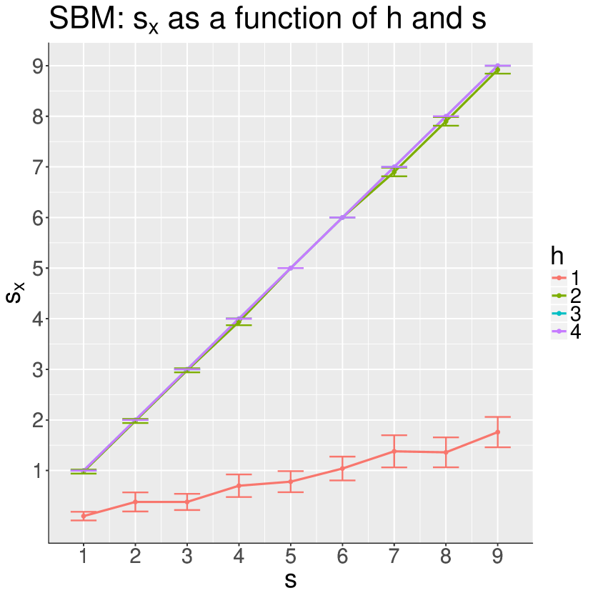
((a)) $SBM(3,b,\Lambda)$ on $300$ vertices, with eqaul block sizes. $\Lambda$ is defines so that the diagonal elements are $0.4$ and the off-diagonal elements are $0.05$.

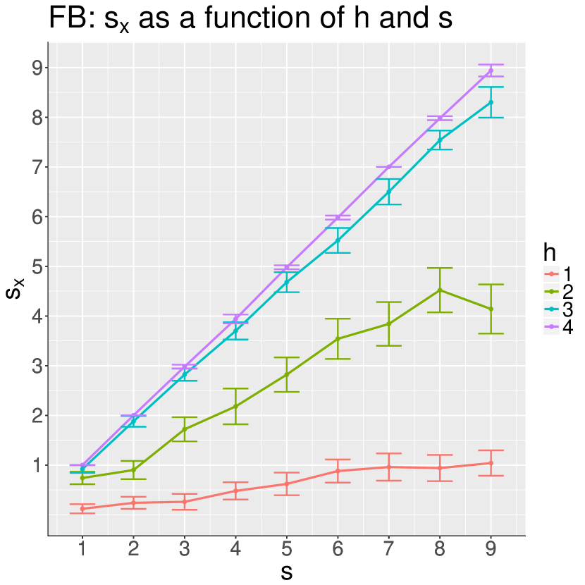
((b)) Facebook network ³⁵.

Figure 1: Average size of $S_{x}$ over 50 Monte Carlo simulations as a function of $(h,s)$; seed sets and vertex of interest selected randomly. As $h$ increases, more vertices in the graph are within an $h$-path of the randomly chosen VOI, and therefore more of the seed vertices are in $N_{h}(x)$.

5 Simulations and real data experiments

Note here that all necessary code and data needed to produce the figures in this section can be found at http://www.cis.jhu.edu/~parky/D3M/VNSGM/.

We will measure the performance of VNmatch via rank$(x^{\prime})$, the expected rank of $x^{\prime}$ in $\Phi_{x}$ when ties are broken uniformly at random. Since the size of the set of candidate matches $C_{x}^{\prime}:=V_{x}^{\prime}\setminus S_{x}^{\prime}$ (seeds in $G^{\prime}$ will never be matched to $x$ by SoftSGM) varies greatly in each experiment, we will compare across experiments by computing the normalized rank of $x^{\prime}$

$$\tau(x^{\prime})=\left(\frac{\text{rank}(x^{\prime})-1}{|C_{x}^{\prime}|-1}\right)\vee 0\in[0,1].$$ (5)

Note that $\tau(x^{\prime})=0$ (resp., $\tau(x^{\prime})=0.5$ or $\tau(x^{\prime})=1$) implies that the $\Phi_{x}(1)=x^{\prime}$ (resp., $\Phi_{x}(|C_{x}^{\prime}|/2)=x^{\prime}$ or $\Phi_{x}(\alpha)=x^{\prime}$ for $\alpha\geq|C_{x}^{\prime}|$); i.e., the VOI was first, half-way down, or effectively last in the nomination list. A low value of $\tau(x^{\prime})$ corresponds to a low ranking of $x^{\prime}$ in the nomination list output from the VNmatch algorithm and corresponds to a measure of how much time is saved (versus a uniformly random search) by the end-user when searching through the candidate set of vertices for the true match $x^{\prime}$. We view a score of $\tau(x^{\prime})=5/100$ as better than a score of $\tau(x^{\prime})=5/10$ since the amount of time saved by the end-user is greater in the first case.

5.1 Simulation experiments

We first explore the performance of Algorithm 2 in the $\rho$-RDPG setting, followed by the $\rho$-SBM setting (see Section 3 for descriptions of these models). To wit, we first generate pairs of graphs from a $\rho\hbox{\sout{ }}RDPG(X)$, where the latent positions of $X$ are uniformly chosen so that each row of $X$ is a unit vector and for any two rows of $X$, namely $X_{i}$ and $X_{j}$, $X_{i}X_{j}^{T}\in(0,1)$. In Figure 2 we explore how $\tau(x^{\prime})$ is affected by the number of seeds used in the matching as compared against various correlation values $\rho=0,0.3,0.5,0.7,1$ (2a) and disparities in the sizes of the graphs to be matched when $\rho=0.6$ (2b).

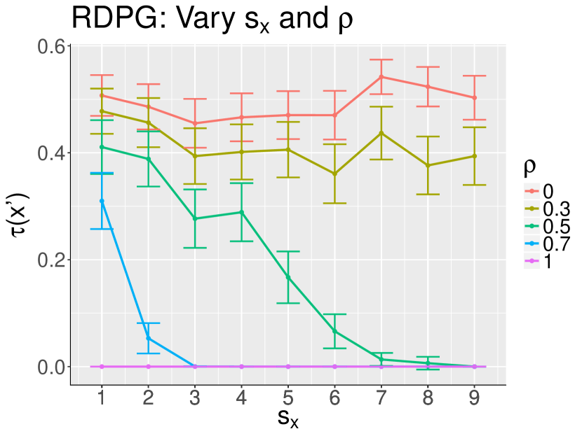
((a)) We plot $\tau(x^{\prime})$ as a function of the number of seeds, $s_{x}$ for various $\rho$.

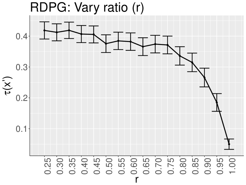
((b)) $\tau(x^{\prime})$ as a function of $r$, the ratio of the vertex sizes of the two graphs, using $s_{x}=4$ and $\rho=0.6$,

Figure 2: For pairs of $300$-node graphs generated from a $\rho\hbox{\sout{ }}RDPG(X)$ model, we plot the average nomralized rank, $\tau(x^{\prime})$, as a function of $s_{x}$, $\rho$, and $r$.

Next, we generate pairs of graphs from a $\rho\hbox{\sout{ }}SBM(3,b,\Lambda)$, where $b$ is such that $1/3$ of the vertices are in each block and

$$\Lambda=\begin{bmatrix}0.7&0.3&0.4\\ 0.3&0.7&0.3\\ 0.4&0.3&0.7\end{bmatrix}.$$ (6)

In Figure 3, we explore how $\tau(x^{\prime})$ is affected by the number of seeds used in the matching as compared against correlation values $\rho=0,0.3,0.5,0.7,1$ (3a) and disparities in the sizes of the graphs to be matched when $\rho=0.6$ (3b).

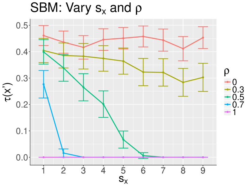
((a)) We plot $\tau(x^{\prime})$ as a function of $s_{x}$ for various $\rho$.

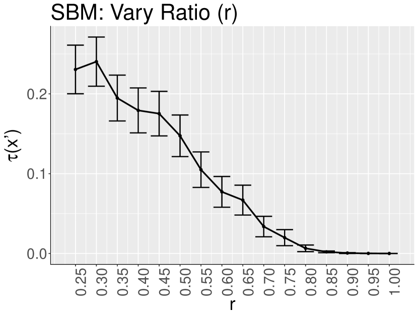
((b)) $\tau(x^{\prime})$ as a function of $r$, the ratio of the vertex sizes of the two graphs, using $s_{x}=4$ and $\rho=0.6$,

Figure 3: For pairs of $300$-node graphs generated from a $\rho\hbox{\sout{ }}SBM(3,b,\Lambda)$, we the average normalized rank, $\tau(x^{\prime})$, as a function of $s_{x}$, $\rho$, and $r$.

In order to explore how the number of seeds used in matching, $s_{x}$, affects the location of the VOI in the nomination list, in both the RDPG and SBM setting, we vary $s_{x}$ from 1 to 9, and run 100 Monte Carlo replicates using VNmatch, with both the VOI and the seeds chosen uniformly at random in each Monte Carlo replicate. In Figures 2a and 3a, we record the average normalized rank of the VOI in the nomination list ($\pm 2$s.e.) for the RDPG and SBM settings, respectively. It is apparent that for sufficiently correlated networks, as the number of seeds increases, our proposed nomination scheme becomes more accurate; i.e., the location of the VOI in the nomination list is closer to the top of the list. For graphs with very low correlation, the uniformly poor performance can be attributed to both the lack of much common structure between $G_{x}$ and $G_{x}^{\prime}$ and the failure of SoftSGM to tease out this common structure. Since both $G$ and $G^{\prime}$ are dense networks, $N_{\ell}(S_{x})$ and $N_{\ell}(S_{x}^{\prime})$ generally contained between 250 and 300 vertices each. Thus, the proportion of shared vertices in $G_{x}$ and $G_{x}^{\prime}$ is rather high for this example.

To explore how the normalized rank of the VOI is influenced by matching graphs which differ in size, we next consider pairs of graphs on different sized vertex sets. We will set the number of vertices in the smaller graph, $G^{\prime}$, to be $|V^{\prime}|=r|V|=300r$, for $r=0.25,0.30,\ldots,1$. Let $H^{\prime}=G^{\prime}$ and suppose there exists an induced subgraph $H$ of $G$ so that $(H,G^{\prime})\sim 0.6\hbox{\sout{ }}RDPG(X)$ for Figure 2b and $(H,G^{\prime})\sim 0.6\hbox{\sout{ }}SBM(3,b,\Lambda)$ for Figure 3b. For each $r$, we plot the average $\tau(x^{\prime})$ ($\pm 2$s.e.) over 100 Monte Carlo replicates for fixed $s_{x}=4$. As can be seen, under this model when the original networks $G$ and $G^{\prime}$ have a large discrepancy between the sizes of their vertex sets there is less accuracy in the VNmatch algorithm. Furthermore, the more obvious community structure present in the SBM setting contributes to better performance of the VNmatch algorithm. Although we are not matching graphs $G_{x}$ and $G_{x}^{\prime}$ with vertex size difference ratio $r$ at every iteration, since the connectivity of the vertices is high, $G_{x}$ and $G_{x}^{\prime}$ do not deviate much from being the full graphs.

Li and Campbell explore the effects of utilizing seeds in graph matching problems in ²⁸. They found that although a small number of seeds can greatly increase the number of correctly matched vertices, as the number of shared users decreases so does the ability to find a good match. As might be expected, since the number of potential mismatches increases as the number of shared users decreases, Figures 2b and 3b are consistent with Li and Campbell’s results.

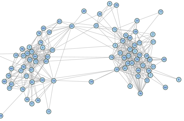
((a)) Facebook

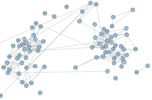
((b)) Survey

Figure 4: The induced subgraphs for the High School Facebook and Survey networks generated by the shared vertices ³⁵.

5.2 Real data experiments

In this section, we explore two applications of VNmatch on real data. Section 5.2.1 explores a pair of high-school networks obtained from ³⁵ in which the first graph is created based on student responses to a ‘who-knows-who’ survey and the second is a Facebook friendship network involving some of the same students. In Section 5.2.2, we consider Instagram and Twitter networks having over-lapping vertex sets in which we would like to identify which Instagram profile corresponds to a particular Twitter profile.

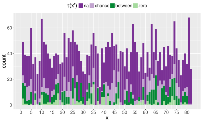
Figure 5: Consider each $x\in V$ as the VOI ($|V|=82$). For each $v\in N_{2}(x)$ match the induced subgraphs of $H$ and $H^{\prime}$ generated by $N_{2}(v)$ and $N_{2}(v^{\prime})$, considering $\{v\}$ and $\{v^{\prime}\}$ to be seed-sets of size $1$. For each $x$, plot how often $\tau(x^{\prime})\in\{0,(0,0.5),[0.5,1],NA\}$ in light green, dark green, light purple, and dark purple, respectively (colors here listed in order as they appear in the plot from bottom to top). The height of the stack represents the total number of vertices in $N_{2}(x)$.

5.2.1 Finding friends in high school networks

We consider two High School friendship networks on over-lapping vertex sets published in ³⁵. The first network, having 156 vertices, represents a Facebook network of profiles in which two vertices are adjacent if the pair of individuals were friends on Facebook. The second network consists of 134 vertices, each representing a particular student, and two vertices are adjacent if one of the students reported that they are friends with the other student. There are 82 shared vertices across the two networks for which we know the bijection between the two vertex sets, and the remaining vertices are known to have no such correspondence. In the language of Section 1, $\eta=156$, $\eta^{\prime}=134$, $n+s=81$, $m=74$, and $m^{\prime}=52$.

Due to the large number of unshared vertices (nearly 40% and 50% for the Survey and Facebook networks, respectively), for illustrative purposes we perform our analysis of this data set by looking at the induced subgraphs generated by the shared vertices. A brief glimpse into the effects of the unshared vertices can be found in the supplemental material accompanying this article. This step is purely for exploratory analysis and would not be feasible in practice, as we would not have prior knowledge about which vertices in the networks are shared as opposed to unshared. At the same time, immediate success of VNmatch is still not guaranteed since the structure of the two graphs is very different, see Figure 4. Furthermore, we can see that there appears to be a 2-block structure for each of the (shared) networks, although, if we were to model these networks the block probability matrices for the two networks appears to differ (unlike our simulation examples).

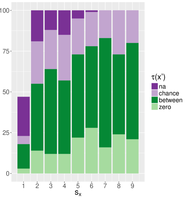
((a)) As a function of $s_{x}$, plot how often $\tau(x^{\prime})\in\{0,(0,0.5),[0.5,1],NA\}$ in light green, dark green, light purple, and dark purple, respectively (colors in order as they appear in plot from bottom to top).

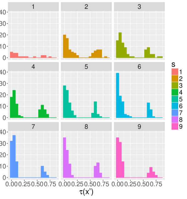
((b)) For each $s_{x}$ we show a bar-chart of $\tau(x^{\prime})$ for each simulation in which $x^{\prime}\in V_{x}^{\prime}$ (i.e., $\tau(x^{\prime})\neq NA$).

Figure 6: Using $x=v_{27}$ as the VOI, vary $s_{x}$ from $1$ to $9$ in VNmatch. For $s_{x}>1$, uniformly at random generate $100$ seed sets from $N_{2}(x)$. For $s_{x}=1$, consider all $47$ possible seed sets of size $1$.

We first explore how VNmatch performs when finding the VOI using a single seed. Let $H$ and $H^{\prime}$ denote, respectively, the induced subgraphs of the High School Facebook and Friendship-Survey networks generated by the $82$ shared vertices. We run $82$ experiments, one for considering each $x\in V$ as the VOI, and for each VOI we consider using each $v\in N_{2}(x)$ as our single seed for VNmatch. In Figure 5, for each $x$, we plot how often $\tau(x^{\prime})\in\{0,(0,0.5),[0.5,1],NA\}$ in light green, dark green, light purple, and dark purple, respectively (colors listed in order as they appear in Figure 5 from bottom to top): When $\tau(x^{\prime})=0$, the true match $x^{\prime}$ is at the top of the nomination list – this is the best case possible; when $\tau(x^{\prime})\in(0,0.5)$, $x^{\prime}$ is somewhere between the top of the nomination list and half-way down (i.e. better than chance, but not first); when $\tau(x^{\prime})\in[0.5,1]$ the nomination list from VNmatch is worse than a uniformly random nomination list; and finally $\tau(x^{\prime})=NA$ means that $x^{\prime}\not\in V_{x}^{\prime}$ and our algorithm cannot hope to nominate the correct vertex. The height of the stack represents the total number of vertices in $N_{2}(x)$. While beyond the scope of this work, this figure points to the impact of seed-selection as well-chosen seeds can be the difference between perfect algorithmic performance and performance worse than chance. Note also that for vertices 6, 31, 36, and 49, $x^{\prime}\not\in V_{x}^{\prime}$ for all $v\in N_{2}(x)$, so, matching the two neighborhoods for these vertices would never be successful for $\ell=h=2$.

We next consider the effects of increasing $s_{x}$. For simplicity, we present our findings while considering vertex 27 to be the VOI. Vertex 27 shows moderately good performance using 1 seed in Figure 5, although not the best. We expect VNmatch to work equally well on any other vertex with similar (or better) performance to vertex 27 as noted in Figure 5.

With vertex $x=v_{27}$ as the VOI in $G$, for each $s_{x}$ increasing from $2$ to $9$ we uniformly at random generate $100$ seed sets from $N_{2}(x)$ and apply VNmatch to match $G_{x}$ and $G_{x}^{\prime}$ using these seed sets. For $s_{x}=1$, rather than having 100 Monte Carlo replicates, we consider only the $47$ possible seed sets of size $1$ in $N_{2}(27)$. Figure 6, displays $\tau(x^{\prime})$ as a function of $s_{x}$, with Figure 6a showing the general performance of $\tau(x^{\prime})$ with respect to $s_{x}$ and Figure 6b displaying a frequency histogram (conditioned on $\tau(x^{\prime})\neq NA$) of $\tau(x^{\prime})$ for each $s_{x}\in\{1,\ldots,9\}$.

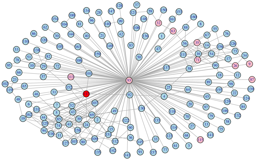
((a)) Twitter

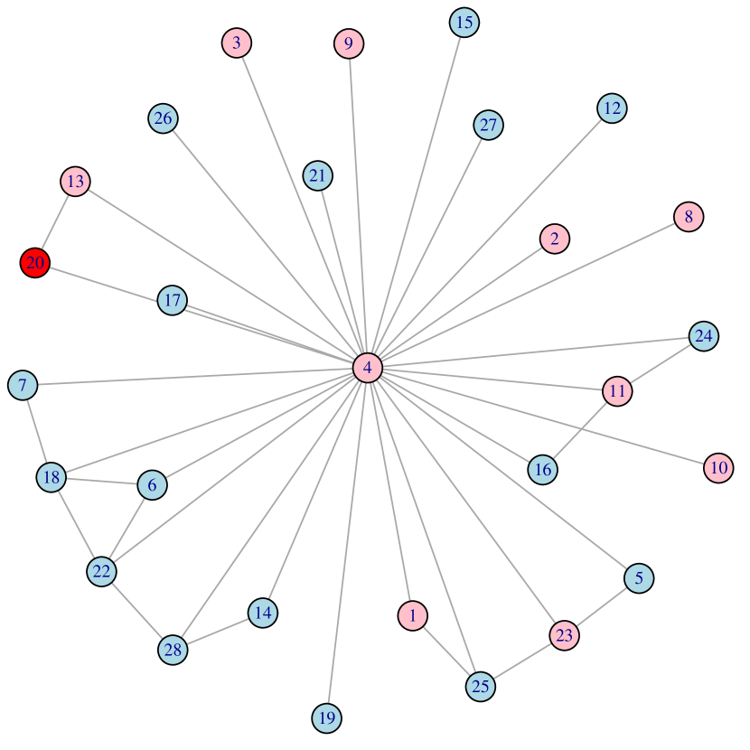
((b)) Instagram

Figure 7: Graphs of a particular friend of the VOI for both Twitter and Instagram; VOI in red and seeds in pink.

5.2.2 Finding Friends on Instagram from Twitter

We next consider nominating across two publicly available social network datasets, one derived from Twitter and one derived from Instagram, where there is an edge between two vertices if one vertex is following the other vertex in the respective social network. We consider a single vertex present on both the Twitter and Instagram networks and construct the two-hop neighborhoods of this vertex in each network, yielding a 163 vertex Twitter graph (Figure 7a) and a 28 vertex Instagram graph (Figure 7b). After identifying a VOI in each network, a simple metadata analysis of vertex features yields 10 potential seeds. In Figure 8, we plot the average value of $\tau(x^{\prime})$ ($\pm 2$s.e.) when using a seed set of size $s_{x}=2,4,6,8,10$. To avoid pathologies arising from $x^{\prime}\not\in V_{x}^{\prime}$, we use vertex 8 as a seed in each experiment. As there are few seeds here, we average $\tau$ over all possible sets of seeds of size $s_{x}$ in each example.

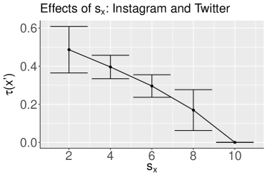
Figure 8: Plot the average value of $\tau(x)$ (Equation 5), along with a confidence bound, for $s_{x}=2,4,6,8,10$, always using the center vertex ($8$) as a seed.

There are a few takeaways from this figure. First note that as the number of seeds increases, the performance of VNmatch increases significantly (i.e., the rank of $x^{\prime}$ in $\Phi_{x}$ is closer to the top). In fact, we find that there are two vertices (including the central vertex in both graphs) whose presence in the seed sets are crucial in that if they are in the seed set then $\tau(x^{\prime})=0$ every time, and if not then $\tau(x^{\prime})>0.5$. Thus, the improvement upon $\tau(x^{\prime})$ in Figure 8 is due to the increased proportion of seed sets which contain the two crucial seeds for identifying the true match. Furthermore, these are the only two seeds which are adjacent to the vertex of interest. This indicates that in the future it may be beneficial to focus on what vertex-properties impact seed-usefulness in terms of assistance with matchability. Also note that these graphs are quite local—the full Twitter and Instagram networks would have $>>10^{7}$ vertices—yet our algorithm still performed quite well only considering $\approx 10^{2}$ vertices. Indeed, by whittling the networks down into local neighborhoods, we are able to leverage the rich local signal present across networks without the computational burden induced by working with the full, often massive, networks themselves.

6 Conclusions

In this paper, we introduce an across-graph vertex nomination scheme based on local neighborhood alignment for identifying a vertex of interest. Our algorithm operates locally within much larger networks, and can scale to be implemented in the very large networks ubiquitous in this age of big data. We demonstrated the efficacy of our principled methodology on both simulated and real data networks, including an application to networks from Twitter and Instagram.

In this paper we have focused on finding a corresponding vertex in a second network to the VOI in the first network with a notion of correspondence in our real-data examples meaning that two nodes across the networks represent the same individual. Another application of this algorithm would be finding vertices, either across two networks or across two subnetworks of one larger network, that have similar structural role across the two networks. Since the resulting nomination list of the VNmatch algorithm already outputs nodes in an ordering that is based on which vertices in a localized version of the second network have similar localized structural role to the VOI in the first network, this extension follows immediately.

In the future, we would like to theoretically and empirically explore the impacts of network correlation and errors on VNmatch for various random graph models. We are also actively seeking to understand the effects of different types of seeds and what makes a “good” seed. The impact of unshared vertices and their connections on the performance of the VNmatch algorithm is still an open area of investigation. Applying VNmatch to multiple VOI could be done either iteratively or simultaneously. Other questions to explore include the addition of attributes and how to apply VNmatch simultaneously across multiple (more than $2$) networks.

Supporting information

Relevant code and data for all simulations and experiments can be found at http://www.cis.jhu.edu/~parky/D3M/VNSGM/.

The high school friendship and Facebook network data was originally published in ³⁵ as data sets three and four, respectively. A detailed description of the data sets can also be found at http://www.sociopatterns.org/datasets/high-school-contact-and-friendship-networks/.

Author Biography

Heather G. Patsolic received the BS degree in mathematics from Wingate University, in 2012, and the MA degree in mathematics from Wake Forest University, in 2014. She is currently a doctoral candidate in the Applied Mathematics and Statistics Department at Johns Hopkins University (JHU). Her research interests include statistical inference for high-dimensional and graph data, model selection, and pattern recognition.

Youngser Park received the BE degree in electrical engineering from Inha University, Seoul, Korea, in 1985, and the MS and PhD degrees in computer science from George Washington University, in 1991 and 2011, respectively. From 1998 to 2000, he worked in the Johns Hopkins Medical Institutes as a senior research engineer. From 2003 until 2011, he worked as a senior research analyst, and has been an associate research scientist since $2011$ in the Center for Imaging Science, Johns Hopkins University (JHU). At JHU, he holds joint appointments in the Institute for Computational Medicine and the Human Language Technology Center of Excellence. His current research interests include clustering algorithms, pattern classification, and data mining for high-dimensional and graph data.

Vince Lyzinski received the BSc degree in mathematics from the University of Notre Dame in 2006, the MSc degree in mathematics from Johns Hopkins University (JHU) in 2007, the MSE degree in applied mathematics and statistics from JHU in 2011, and the PhD degree in applied mathematics and statistics from JHU, in 2013. From 2013 to 2014, he was a postdoctoral fellow in the Applied Mathematics and Statistics (AMS) Department, JHU, and from 2014 to 2017, he was a senior research scientist in the JHU Human Language Technology Center of Excellence and an assistant research professor in the AMS Department, JHU. From 2017 to 2019 he was an assistant professor in the Department of Mathematics and Statistics at the University of Massachusetts, Amherst. Since 2019 he has been an assistant professor in the Department of Mathematics at the University of Maryland, College Park. His research interests include graph matching, statistical inference on random graphs, pattern recognition, dimensionality reduction, stochastic processes, and high-dimensional data analysis.

Carey E. Priebe received the BS degree in mathematics from Purdue University in 1984, the MS degree in computer science from San Diego State University, in 1988, and the PhD degree in information technology (computational statistics) from George Mason University, in 1993. From 1985 to 1994, he worked as a mathematician and scientist in the US Navy research and development laboratory system. Since 1994, he has been a professor in the Department of Applied Mathematics and Statistics, Johns Hopkins University (JHU). At JHU, he holds joint appointments in the Department of Computer Science, Department of Electrical and Computer Engineering, Center for Imaging Science, Human Language Technology Center of Excellence, and Whitaker Biomedical Engineering Institute. His research interests include computational statistics, kernel and mixture estimates, statistical pattern recognition, statistical image analysis, dimensionality reduction, model selection, and statistical inference for high-dimensional and graph data. He is a lifetime member of the IMS, an elected member of the ISI, and a fellow of the ASA.

References

- Airoldi et al. 2008 Airoldi, E. M., D. M. Blei, S. E. Fienberg, and E. P. Xing, 2008: Mixed membership stochastic blockmodels. The Journal of Machine Learning Research, 9, 1981–2014.
- Berg et al. 2005 Berg, A., T. Berg, and M. J., 2005: Shape matching and object recognition using low distortion correspondences. 2005 IEEE Conference on Computer Vision and Pattern Recognition, 26–33.
- Bergsma and Van Durme 2013 Bergsma, S. and B. Van Durme, 2013: Using conceptual class attributes to characterize social media users. Proceedings of the 51st Annual Meeting of the Association for Computational Linguistics (Volume 1: Long Papers), 710–720.
- Beveridge 1994 Beveridge, J. R., 1994: Local search algorithms for geometric object recognition: Optimal correspondence and pose.
- Conte et al. 2004 Conte, D., P. Foggia, C. Sansone, and M. Vento, 2004: Thirty years of graph matching in pattern recognition. International Journal of Pattern Recognition and Artificial Intelligence, 18, no. 3, 265–298.
- Coppersmith 2014 Coppersmith, G., 2014: Vertex nomination. Wiley Interdisciplinary Reviews: Computational Statistics, 6, no. 2, 144–153.
- Coppersmith and Priebe 2012 Coppersmith, G. and C. Priebe, 2012: Vertex nomination via content and context. arXiv preprint arXiv:1201.4118.
- Devroye et al. 2013 Devroye, L., L. Györfi, and G. Lugosi, 2013: A probabilistic theory of pattern recognition, volume 31. Springer Science & Business Media.
- Fabiana et al. 2015 Fabiana, C., M. Garetto, and E. Leonardi, 2015: De-anonymizing scale-free social networks by percolation graph matching. Computer Communications (INFOCOM), 2015 IEEE Conference on, IEEE, 1571–1579.
- Fiori et al. 2013 Fiori, M., P. Sprechmann, J. Vogelstein, P. Musé, and G. Sapiro, 2013: Robust multimodal graph matching: Sparse coding meets graph matching. Advances in Neural Information Processing Systems, 127–135.
- Fishkind et al. 2019 Fishkind, D., S. Adali, H. Patsolic, L. Meng, D. Singh, V. Lyzinski, and C. Priebe, 2019: Seeded graph matching. Pattern Recognition, 87, 203–215.
- Fishkind et al. 2015 Fishkind, D., V. Lyzinski, H. Pao, L. Chen, and C. Priebe, 2015: Vertex nomination schemes for membership prediction. The Annals of Applied Statistics, 9, no. 3, 1510–1532.
- Foggia et al. 2014 Foggia, P., G. Perncannella, and M. Vento, 2014: Graph matching and learning in pattern recognition in the last 10 years. Internation Journal of Pattern Recognition and Artificial Intelligence, 28, no. 1.
- Frank and Wolfe 1956 Frank, M. and P. Wolfe, 1956: An algorithm for quadratic programming. Naval Research Logistics Quarterly, 3, 95–110, doi:10.1002/nav.3800030109.
- Fukunage and Narendra 1975 Fukunage, K. and P. M. Narendra, 1975: A branch and bound algorithm for computing k-nearest neighbors. IEEE transactions on computers, no. 7, 750–753.
-
Gönen and Alpaydin 2008
Gönen, M. and E. Alpaydin, 2008: Localized multiple kernel learning. Proceedings of the 25th International Conference on Machine Learning, ACM,
New York, NY, USA, ICML ’08, 352–359.
URL http://doi.acm.org/10.1145/1390156.1390201 - Ham et al. 2005 Ham, J., D. D. Lee, and L. K. Saul, 2005: Semisupervised alignment of manifolds. AISTATS, 120–127.
- Holland et al. 1983 Holland, P. W., K. Laskey, and S. Leinhardt, 1983: Stochastic blockmodels: First steps. Social Networks, 5, no. 2, 109–137.
- Huang et al. 2004 Huang, Z., W. Chung, and H. Chen, 2004: A graph model for e-commerce recommender systems. Journal of the American Society for information science and technology, 55, no. 3, 259–274.
- Ji et al. 2016 Ji, S., W. Li, S. Yang, P. Mittal, and R. Beyah, 2016: On the relative de-anonymizability of graph data: Quantification and evaluation. Computer Communications, IEEE INFOCOM 2016-The 35th Annual IEEE International Conference on, IEEE, 1–9.
- Kazemi et al. 2015a Kazemi, E., S. H. Hassani, and M. Grossglauser, 2015a: Growing a graph matching from a handful of seeds. Proceedings of the VLDB Endowment, 8, no. 10, 1010–1021.
- Kazemi et al. 2015b Kazemi, E., L. Yartseva, and M. Grossglauser, 2015b: When can two unlabeled networks be aligned under partial overlap? Communication, Control, and Computing (Allerton), 2015 53rd Annual Allerton Conference on, IEEE, 33–42.
- Keller et al. 1985 Keller, J. M., M. R. Gray, and J. A. Givens, 1985: A fuzzy k-nearest neighbor algorithm. IEEE transactions on systems, man, and cybernetics, no. 4, 580–585.
- Kuchaiev and Pržulj 2011 Kuchaiev, O. and N. Pržulj, 2011: Integrative network alignment reveals large regions of global network similarity in yeast and human. Bioinformatics, 27, no. 10, 1390–1396.
- Kuhn 1955 Kuhn, H., 1955: The hungarian method for the assignment problem. Naval Research Logistics Quarterly, 2, 83–97, doi:10.1002/nav.3800020109.
- Leordeanu et al. 2012 Leordeanu, M., R. Sukthankar, and M. Hebert, 2012: Unsupervised learning for graph matching. International Journal of Computer Vision, 96, no. 1, 28–45.
- Leskovec and Krevl 2014 Leskovec, J. and A. Krevl, 2014: SNAP Datasets: Stanford large network dataset collection. http://snap.stanford.edu/data.
- Li and Campbell 2015 Li, L. and W. Campbell, 2015: Matching community structure across online social networks. Networks NIPS.
- Lyzinski et al. 2016a Lyzinski, V., D. Fishkind, M. Fiori, J. Vogelstein, C. Priebe, and G. Sapiro, 2016a: Graph matching: Relax at your own risk. IEEE Transactions on Pattern Analysis and Machine Intelligence, 38, no. 1, 60–73.
- Lyzinski et al. 2014 Lyzinski, V., D. Fishkind, and C. Priebe, 2014: Seeded graph matching for correlated Erds-Rènyi graphs. Journal of Machine Learning Research, 15, no. Nov, 3693–3720.
- Lyzinski et al. 2016b Lyzinski, V., K. Levin, D. E. Fishkind, and C. E. Priebe, 2016b: On the consistency of the likelihood maximization vertex nomination scheme: Bridging the gap between maximum likelihood estimation and graph matching. Journal of Machine Learning Research, 17, no. 179, 1–34.
- Lyzinski et al. 2019 Lyzinski, V., K. Levin, and C. E. Priebe, 2019: On consistent vertex nomination schemes. Journal of Machine Learning Research, 20, no. 69, 1–39.
- Lyzinski et al. 2015 Lyzinski, V., D. L. Sussman, D. E. Fishkind, H. Pao, L. Chen, J. T. Vogelstein, Y. Park, and C. E. Priebe, 2015: Spectral clustering for divide-and-conquer graph matching. Parallel Computing, 47, 70–87.
- Marchette et al. 2011 Marchette, D., C. E. Priebe, and G. Coppersmith, 2011: Vertex nomination via attributed random dot product graphs. Proceedings of the 57th ISI World Statistics Congress, volume 6, 16.
- Mastrandrea et al. 2015 Mastrandrea, R., J. Fournet, and A. Barrat, 2015: Contact patterns in a high school: a comparison between data collected using wearable sensors, contact diaries and friendship surveys. PLoS ONE, doi:10.1371/journal.pone.0136497.
- Milenkovic et al. 2010 Milenkovic, T., W. Ng, W. Hayes, and N. Pržulj, 2010: Optimal network alignment with graphlet degree vectors. Cancer Informatics, 9, 121.
- Muja and Lowe 2009 Muja, M. and D. G. Lowe, 2009: Fast approximate nearest neighbors with automatic algorithm configuration. VISAPP (1), 2, no. 331-340, 2.
- Olhede and Wolfe 2014 Olhede, S. C. and P. J. Wolfe, 2014: Network histograms and universality of block model approximation. Proceedings of the National Academy of Sciences, 111, 14722–14727.
- Page et al. 1999 Page, L., S. Brin, R. Motwani, and T. Winograd, 1999: The pagerank citation ranking: Bringing order to the web. Stanford InfoLab.
- Pedarsani et al. 2013 Pedarsani, P., D. R. Figueiredo, and M. Grossglauser, 2013: A bayesian method for matching two similar graphs without seeds. Communication, Control, and Computing (Allerton), 2013 51st Annual Allerton Conference on, IEEE, 1598–1607.
- Priebe et al. 2005 Priebe, C. E., J. M. Conroy, D. J. Marchette, and Y. Park, 2005: Scan statistics on enron graphs. Computational & Mathematical Organization Theory, 11, no. 3, 229–247.
- Priebe et al. 2019 Priebe, C. E., Y. Park, J. T. Vogelstein, J. M. Conroy, V. Lyzinski, M. Tang, A. Athreya, J. Cape, and E. Bridgeford, 2019: On a two-truths phenomenon in spectral graph clustering. 116, no. 13, 5995–6000, doi:10.1073/pnas.1814462116.
- Rastogi et al. 2017 Rastogi, P., V. Lyzinski, and B. Van Durme, 2017: Vertex nomination on the cold start knowledge graph. Human Language Technology Center of Excellence: Technical report.
- Rohe et al. 2011 Rohe, K., S. Chatterjee, and B. Yu, 2011: Spectral clustering and the high-dimensional stochastic blockmodel. Annals of Statistics, 39, 1878–1915.
- Sen et al. 2008 Sen, P., G. Namata, M. Bilgic, L. Getoor, B. Galligher, and T. Eliassi-Rad, 2008: Collective classification in network data. AI magazine, 29, no. 3, 93–93.
- Sermanet et al. 2013 Sermanet, P., D. Eigen, X. Zhang, M. Mathieu, R. Fergus, and Y. LeCun, 2013: Overfeat: Integrated recognition, localization and detection using convolutional networks. arXiv preprint arXiv:1312.6229.
- Stone 1977 Stone, C. J., 1977: Consistent nonparametric regression. The annals of statistics, 595–620.
- Sun et al. 2012 Sun, M., M. Tang, and C. E. Priebe, 2012: A comparison of graph embedding methods for vertex nomination. 2012 IEEE ICMLA, volume 1, 398–403.
- Sussman et al. 2012 Sussman, D. L., M. Tang, D. E. Fishkind, and C. E. Priebe, 2012: A consistent adjacency spectral embedding for stochastic blockmodel graphs. Journal of the American Statistical Association, 107, no. 499, 1119–1128.
- Suwan et al. 2015 Suwan, S., D. S. Lee, and C. E. Priebe, 2015: Bayesian vertex nomination using content and context. Wiley Interdisciplinary Reviews: Computational Statistics, 7, no. 6, 400–416.
- Talukdar and Pereira 2010 Talukdar, P. P. and F. Pereira, 2010: Experiments in graph-based semi-supervised learning methods for class-instance acquisition. Proceedings of the 48th annual meeting of the association for computational linguistics, Association for Computational Linguistics, 1473–1481.
- Vogelstein et al. 2015 Vogelstein, J., J. Conroy, V. Lyzinski, L. Podrazik, S. Kratzer, E. Harley, D. Fishkind, R. Vogelstein, and C. Priebe, 2015: Fast approximate quadratic programming for graph matching. PLOS one, 10, no. 4, e0121002.
- Wang et al. 2013 Wang, H., M. Tang, Y. Park, and C. E. Priebe, 2013: Locality statistics for anomaly detection in time series of graphs. IEEE Transactions on Signal Processing, 62, no. 3, 703–717.
- Wiskott et al. 1997 Wiskott, L., N. Fellous, J-M.and Krüger, and C. Malsburg, 1997: Face recognition by elastic bunch graph matching. IEEE Transactions on Pattern Analysis and Machine Intelligence, 19, no. 7, 775–779.
- Yan et al. 2013 Yan, J., Y. Tian, H. Zha, X. Yang, Y. Zhang, and S. Chu, 2013: Joint optimization for consistent multiple graph matching. Proceedings of the IEEE International Conference on Computer Vision, 1649–1656.
- Young and Scheinerman 2007 Young, S. J. and E. R. Scheinerman, 2007: Random dot product graph models for social networks. International Workshop on Algorithms and Models for the Web-Graph, Springer, 138–149.
- Zaslavskiy et al. 2009a Zaslavskiy, M., F. Bach, and J.-P. Vert, 2009a: Global alignment of protein–protein interaction networks by graph matching methods. Bioinformatics, 25, no. 12, i259–1267.
- Zaslavskiy et al. 2009b — 2009b: A path following algorithm for the graph matching problem. IEEE Transactions on Pattern Analysis and Machine Intelligence, 31, no. 12, 2227–2242.
- Zass and Shashua 2008 Zass, R. and A. Shashua, 2008: Probabilistic graph and hypergraph matching. Computer Vision and Pattern Recognition, 2008. CVPR 2008. IEEE Conference on, IEEE, 1–8.
- Zhou and De la Torre 2012 Zhou, F. and F. De la Torre, 2012: Factorized graph matching. 2012 IEEE Conference on Computer Vision and Pattern Recognition (CVPR), 127–134.