Dynamic Space Efficient Hashing

Abstract

We consider space efficient hash tables that can grow and shrink dynamically and are always highly space efficient, i.e., their space consumption is always close to the lower bound even while growing and when taking into account storage that is only needed temporarily. None of the traditionally used hash tables have this property. We show how known approaches like linear probing and bucket cuckoo hashing can be adapted to this scenario by subdividing them into many subtables or using virtual memory overcommitting. However, these rather straightforward solutions suffer from slow amortized insertion times due to frequent reallocation in small increments.

Our main result is DySECT (Dynamic Space Efficient Cuckoo Table) which avoids these problems. DySECT consists of many subtables which grow by doubling their size. The resulting inhomogeneity in subtable sizes is equalized by the flexibility available in bucket cuckoo hashing where each element can go to several buckets each of which containing several cells. Experiments indicate that DySECT works well with load factors up to 98%. With up to 2.7 times better performance than the next best solution.

1 Introduction

Dictionaries represented as hash tables are among the most frequently used data structures and often play a critical role in achieving high performance. Having several compatible implementations, which perform well under different conditions and can be interchanged freely, allows programmers to easily adapt known solutions to new circumstances.

One aspect that has been subject to much investigation is space efficiency [3, 4, 7, 8, 17, 19]. Modern space efficient hash tables work well even when filled to 95% and more. To reach filling degrees like this, the table has to be initialized with the correct final capacity, thereby, requiring programmers to know tight bounds on the maximum number of inserted elements. This is typically not realistic. For example, a frequent application of hash tables aggregates information about data elements by their key. Whenever the exact number of unique keys is not known a priori, we have to overestimate the initial capacity to guarantee good performance. Dynamic space efficient data structures are necessary to guarantee both good performance and low overhead independent of the circumstances.

To visualize this, assume the following scenario. During a word count benchmark, we know an upper bound $n_{\max}$ to the number of unique words. Therefore, we construct a hash table with at least $n_{\max}$ cells. If an instance only contains $0.7\cdot n_{max}$ unique words, no static hash table can fill ratios greater than 70%. Thus, dynamic space efficient hash tables are required to achieve guaranteed near-optimal memory usage. In scenarios where the final size is not known, the hash table has to grow closely with the actual number of elements. This cannot be achieved efficiently with any of the current techniques used for hashing and migration.

Many libraries – even ones that implement space efficient hash tables – offer some kind of growing mechanism. However, all existing implementations either lose their space efficiency or suffer from degraded performance once the table grows above its original capacity. Growing is commonly implemented either by creating additional hash tables – decreasing performance especially for lookups or by migrating all elements to a new table – losing the space efficiency by multiplying the original size.

To avoid the memory overhead of full table migrations, during which both the new and the old table coexist, we propose an in-place growing technique that can be adapted to most existing hashing schemes. However, frequent migrations with small relative size changes remain necessary to stay space efficient at all times.

To avoid both of these pitfalls we propose a variant of (multi-way) bucket cuckoo hashing [7, 8]. A technique where each element can be stored in one of several associated constant sized buckets. When all of them are full, we move an element into one of its other buckets to make space. To solve the problem of efficient migration, we split the table into multiple subtables, each of which can grow independently of all others. Because the buckets associated with one element are spread over the different subtables, growing one subtable alleviates pressure from all others by allowing moves from a dense subtable to the newly-grown subtable.

Doubling the size of one subtable increases the overall size only by a small factor while moving only a small number of elements. This makes the size changes easy to amortize. The size and occupancy imbalance between subtables (introduced by one subtable growing) is alleviated using displacement techniques common to cuckoo hashing. This allows our table to work efficiently at fill rates exceeding 95%.

We begin our paper by presenting some previous work (Section 2). Then we go into some notations (Section 3) that are necessary to describe our main contribution DySECT (Section 4). In Section 5 we show our in-place migration techniques. Afterwards, we test all hash tables on multiple benchmarks (Section 6) and draw our conclusion (Section 7)

2 Related Work

The use of hash tables and other hashing based algorithms has a long history in computer science. The classical methods and results are described in all major algorithm textbooks [14].

Over the last one and a half decades, the field has regained attention, both from theoretical and the practical point of view. The initial innovation that sparked this attention was the idea that storing an element in the less filled of two “random” chains leads to incredibly well balanced loads. This concept is called the power of two choices [16].

It led to the development of cuckoo hashing [19]. Cuckoo hashing extends the power of two choices by allowing to move elements within the table to create space for new elements (see Section 3.2 for a more elaborated explanation). Cuckoo hashing revitalized research into space efficient hash tables. Probabilistic bounds for the maximum fill degree [3, 4] and expected displacement distances [9, 10] are often highly non-trivial.

Cuckoo hashing can be naturally generalized into two directions in order to make it more space efficient: allowing $H$ choices [8] or extending cells in the table to buckets that can store $B$ elements. We will summarize this under the term bucket cuckoo hashing.

Further adaptations of cuckoo hashing include:multiple concurrent implementations either powered by bucket locking, transactional memory [15], or fully lock-less [18]; a de-amortization technique that provides provable worst case guarantees for insertions [1, 13]; and a variant that minimizes page-loads in a paged memory scenario [6].

Some non-cuckoo space efficient hash tables continue to use linear probing variants. Robin Hood hashing is a technique that was originally introduced in 1985 [2]. The idea behind Robin Hood hashing is to move already stored elements during insertions in a way that minimizes the longest possible search distance. Robin Hood hashing has regained some popularity in recent years, mainly for its interesting theoretical properties and the possibility to reduce the inherent variance of linear probing.

All these publications show that there is a clear interest in developing hash tables that can be more and more densely filled. Dynamic hash tables on the other hand seem to be considered a solved problem. One paper that takes on the problem of dynamic hash tables was written by Dietzfelbinger at al. [5]. It predates cuckoo hashing, and much of the attention for space efficient hashing. All memory bounds presented are given without tight constant factors. The lack of implementations and theory about dense dynamic hash tables is where we pick up and offer a fast hash table implementation that supports dynamic growing with tight space bounds.

3 Preliminaries

A hash table is a data structure for storing key-value-pairs ($\langle key,data\rangle$) that offers the following functionality: insert – stores a given key-value pair or returns a reference to it, if it is already contained; find – given a key returns an reference to said element if it was stored, and $\bot$ otherwise; and erase – removes a previously inserted element (if present).

Throughout this paper $n$ denotes the number of elements and $m$ the number of cells ($m>n$) in a hash table. We define the load factor as $\delta=n/m$. Tables can usually only operate efficiently up to a certain maximum load factor. Above that, operations get slower or have a possibility to fail. When implementing a hash table one has to decide between storing elements directly in the hash table – Closed Hashing – or storing pointers to elements – Open Hashing. This has an immediate impact on the amount of memory required (closed: $m\cdot|\textit{element}|$ and open: $m\cdot|\textit{pointer}|+n\cdot|\textit{element}|$).

For large elements (i.e., much larger then the size of a pointer), one can use a non-space efficient hash table with open hashing to reduce the relevant memory factor. Therefore, we restrict ourselves to the common and more interesting case of elements whose size is close to that of a pointer. For our experiments we use 128bit elements (64bit keys and 64bit values). In this case, open hashing introduces a significant memory overhead (at least $1.5\times$). For this reason, we only consider closed hash tables. Their memory efficiency is directly dependent on the table’s load. To reach high fill degrees with closed hashing tables, we have to employ open addressing techniques. This means that elements are not stored in predetermined cells, but can be stored in one of several possible places (e.g. linear probing, or cuckoo hashing).

3.1 $\alpha$-Space Efficient Hash Tables

Static.

We call a hashing technique $\alpha$-space efficient when it can work effectively using at most $\alpha\cdot n_{\textit{curr}}\cdot\textit{size}(\textit{element})+O(1)$ memory. In this case we define working efficiently as having average insertion times in $O(\frac{1}{1-\delta})$. This is a natural estimation for insertion times, since it is the expected number of fully random probes needed to hit an empty cell ($1-\delta$ is the fraction of empty cells).

In many closed hashing techniques (e.g. linear probing, cuckoo hashing) cells are the same size as elements. Therefore, being $\alpha$-space efficient is the same as operating with a load factor of $\delta=\alpha^{-1}$. Because of this, we will mostly talk about the load factor of a table instead of its memory usage.

Dynamic.

The definition of a space efficient hashing technique given above is specifically targeted for statically sized hash tables. We call an implementation dynamically $\alpha$-space efficient if an instantiated table can grow arbitrarily large over its original capacity while remaining smaller than $\alpha\cdot n_{\max}\cdot\textit{size}(\textit{element})+O(1)$ at all times.

One problem for many implementations of space efficient hash tables is the migration. During a normal full table migration, both the original table and the new table are allocated. This requires $m_{\textit{new}}+m_{\textit{old}}$ cells. Therefore, a normal full table migration is never more than 2-space efficient. The only option for performing a full table migration with less memory is to increase the memory in-place (see Section 5). Similar to static $\alpha$-space efficiency, we will mostly talk about the minimum load factor $\delta_{\min}=\frac{1}{\alpha}$ instead of $\alpha$.

3.2 Cuckoo Hashing

Cuckoo hashing is a technique to resolve hash conflicts in a hash table using open addressing. Its main draw is that it guarantees constant lookup times even in densely filled tables. The distinguishing technique of cuckoo hashing is that $H$ hash functions ($h_{1},...,h_{H}$) are used to compute $H$ independent positions. Each element is stored in one of its positions. Even if all positions are occupied one can often move elements to create space for the current element. We call this process displacing elements.

Bucket cuckoo hashing is a variant where the cells of the hash table are grouped into buckets of size $B$ ($m/B$ buckets). Each element assigned to one bucket can be stored in any of the bucket’s cells. Using buckets one can drastically increase the number of elements that can be displaced to make room for a new one, thus decreasing the expected length of displacement paths.

Find and erase operations have a guaranteed constant running time. Independent from the table’s density, there are $H$ buckets – $H\cdot B$ cells – that have to be searched to find an element.

During an insert the element is hashed to $H$ buckets. We store the element in the bucket with the most free space. When all buckets are full we have to move elements within the table such that a free cell becomes available.

To visualize the problem of displacing elements, one can think of the directed graph implicitly defined by the hash table. Each bucket corresponds to a node and each element induces an edge between the bucket it is stored in and its $H-1$ alternate buckets. To insert an element into the hash table we have to find a path from one of its associated buckets to a bucket that has free capacity. Then we move elements along this path to make room in the initial bucket. The two common techniques to find such paths are random walks and breadth first searches.

4 DySECT (Dynamic Space Efficient Cuckoo Table)

A commonly used growing technique is to double the size of a hash table by migrating all its elements into a table with twice its capacity. This is of course not memory efficient. The idea behind our dynamic hashing scheme is to double only parts of the overall data structure. This increases the space in part of our data structure without changing the rest. We then use cuckoo displacement techniques to make this additional memory reachable from other parts of the hash table.

4.1 Overview

Our DySECT hash table consists of $T$ subtables (shown in Figure 1) that in turn consist of buckets, which can store $B$ elements each. Each element has $H$ associated buckets – similar to cuckoo hashing – which can be in the same or in different subtables. $T$, $B$, and $H$ are constant that will not change during the lifetime of the table. Additionally, each table is initialized with a minimum fill ratio $\delta_{\min}$. The table will never exceed $\delta_{\min}^{-1}\cdot n$ cells once it begins to grow over its initial size.

To find a bucket associated with an element $e$, we compute $e$’s hash value using the appropriate hash function $h_{i}(e)$. The hash is then used to compute the subtable and the bucket within that subtable. To make this efficient we use powers of two for the number of subtables ($T=2^{t}$), as well as for the number of buckets per subtable (subtable size $s=2^{x}\cdot B$). Since the number of subtables is constant, we can use the first $t$ bits from the hashed key to find the appropriate subtable. From the remaining bits we compute the bucket within that subtable using a bitmask ($h_{i}(e)\,\texttt{\&}\,(2^{x}-1)=h_{i}(e)\mod 2^{x}$).

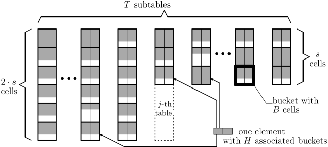
Figure 1: Schematic Representation of a DySECT Table.

4.2 Growing

As soon as the (overall) table contains enough elements such that the memory constraint can be kept during a subtable migration, we grow one subtable by migrating it into a table twice its size. We migrate subtables in order from first to last. This ensures that no subtable can be more than twice as large as any other.

Assume that we have $j$ large subtables ($2s$) than $m=(T+j)\cdot s$. When $\delta_{\min}^{-1}\cdot n>m+2s$ we can grow the first subtable while obeying the size constraint (the newly allocated table will have $2s$ cells). Doubling the size of a subtable increases the global number of cells from $m_{\textit{old}}=(T+j)\cdot s$ to $m_{new}=m_{old}+s=(T+j+1)\cdot s$ (grow factor $\frac{T+j+1}{T+j}$). Note that all subsequent growing operations migrate one of the smaller tables until all tables have the same size. Therefore, each grow until then increases the overall capacity by the same absolute amount (smaller relative to the current size).

The cost of growing a subtable is amortized by all insertions since the last subtable migration. There are $\delta_{\min}\cdot s=\Omega(s)$ insertions between two migrations. One migration takes $\Theta(s)$ time. Apart from being amortized, the migration is cache efficient since it accesses cells in a linear fashion. Even in the target table cells are accessed linearly. We assign elements to buckets by using bits from their hash value. In the grown table we use exactly one more bit than before (double the number of buckets). This ensures that all elements from one original bucket are split between two buckets in the target table. Therefore no bucket can overflow and no displacements are necessary.

In the implicit graph model of the cuckoo table (Section 3.2), growing a subtable is equivalent to splitting each node that represents a bucket within that subtable. The resulting graph becomes more sparse, since the edges (elements) are not doubled, making it easier to insert subsequent elements.

4.3 Shrinking

If shrinking is necessary it can work similarly to growing. We replace a subtable with a smaller one by migrating elements from one to the other. During this migration we join elements from two buckets into one. Therefore it is possible for a bucket to overfill. We reinsert these elements at the end of the migration. Obviously, this can only affect at most half the migrated elements.

When automatically triggering the size reduction, one has to make sure that the migration cost is amortized. Therefore, a grow operation cannot immediately follow a shrink operation. When shrinking is enabled we propose to shrink one subtable when $\delta_{\min}^{-1}\cdot n<m-s^{\prime}$ elements ($s^{\prime}$ size of a large table, $m_{\textit{new}}=m_{\textit{old}}-s^{\prime}/2$). Alternatively, one could implement a shrink to size operation that is explicitly called by the user.

4.4 Difficulties for the Analysis of DySECT

There are two factors specific to DySECT impacting its performance: inhomogeneous table resolution and element imbalance.

Imbalance through Inhomogeneous Table Resolution.

By growing subtables individually we introduce a size imbalance between subtables. Large subtables contain more buckets but the number of elements hashed to a large subtable is not generally higher than the number of elements that are hashed to a small subtable. This makes it difficult to spread elements evenly among buckets. Imbalanced bucket fill ratios can lead to longer insertion times.

Assume there are $n$ elements in a hash table with $T$ subtables, $j$ of which have size $2s$ the others have size $s$. If elements are spread equally among buckets then all small tables have around $n/(T+j)$ elements, and the bigger tables have $2n/(T+j)$ elements. For each table there are about $Hn/T$ elements that have an associated bucket within that table. This shows that having more hash functions can lead to a better balance.

For two hash functions ($H=2$) and only one grown table ($j=1$) this means that $\approx 2n/(T+1)$ elements should be stored in the first table to achieve a balanced bucket distribution. Therefore, nearly all elements associated with a bucket in the first table ($\approx 2n/T$) have to be stored there. This is one reason why $H=2$ does not work well in practice.

Imbalance through Size Changes.

In addition to the problem of inhomogeneous tables there is an inherent balancing problem introduced by resizing subtables. It is clear that a newly grown table is not filled as densely as other tables. Since we double the table size, grown tables can only be filled to about 50%.

Assume the global table is filled close to 100% when the first table grows. Now there is capacity for $s$ new elements but this capacity is only in the first table, elements that are not hashed to the first table, automatically trigger displacements leading to slow insertions. Notice that repeated insert and erase operations help to equalize this imbalance, because elements are more likely inserted into the sparser areas, and more likely to be deleted from denser areas.

4.5 Implementation Details

For our experiments (Section 6) we use three hash functions ($H=3$) and a bucket size of ($B=8$). These values have consistently outperformed other options both in maximum load factor and in insert performance (see Appendix A). $T$ is set to 256 subtables for all our tests. To find displacement opportunities we use breadth first search. In our tests it performed better than random walks, since it better uses the read cache lines from one bucket.

The hash table itself is implemented as a constant sized array of pointers to subtables. We have to lookup the corresponding pointer whenever a subtable is accessed. This does not impact performance much since all subtable pointers will be cached – at least if the hash table is a performance bottleneck.

Reducing the Number of Computed Hash Functions.

Evaluating hash functions is expensive, therefore, reducing the number of hash functions computed per operation can increase the performance of the table. The hash function we use computes 64bit hash values (i.e. xxHash). We split the 64bit hash value into two 32bit values. All common bucket hash table sizes can be addressed using 32 bits (up to $2^{32}$ buckets $2^{35}\approx 34$ billion elements consuming 512GiB memory).

When $H>2$ we can use double hashing [11, 12] to further reduce the number of computed hash functions. Double hashing creates an arbitrary number of hash values using only two original hash functions $h^{\prime}$ and $h^{\prime\prime}$. The additional values are linear combinations computed from the original two values, $h_{i}(key)=h^{\prime}(key)+i\cdot h^{\prime\prime}(key)$.

Combining both of these techniques, we can reduce the number of computed hash functions to one 64bit hash function. This is especially important during large displacements where each encountered element has to be rehashed to find its alternative buckets.

5 (Ab)Using Virtual Memory

In this section we show how one can use virtual memory and memory overcommitting, to eliminate the indirections from a DySECT hash table. The same technique also allows us to implement hash tables that can grow using an in-place full table migration. If we grow these tables in small increments, they can grow while enforcing a strict size constraint.

To explain these techniques, we first have to explain how to use memory overcommitting and virtual memory to create a piece of memory that can grow in-place. Note that this technique violates best programming practices and is not fully portable to some systems.

The idea is the following: the operating system will – if configured to do so – allow memory allocations larger than the machine’s main memory, with the anticipation that not all allocated memory will actually be used. Only memory pages that are actually used will be mapped from virtual to physical memory pages. Thus, for the purpose of space efficiency the memory is not yet used. Initializing parts of this memory is similar to allocating and initializing new memory.

5.1 Improving DySECT

Accessing a DySECT subtable usually takes one indirection. The pointer to the subtable has to be read from an array of pointers before accessing the actual subtable. Instead of using an array of pointers, we can implement the subtables as sections within one large allocation (size $u$). We choose $u$ larger than the actual main memory, to allow all possible table sizes. This has the advantage that the offset for each table can be computed quickly ($t_{i}=\frac{u}{T}\cdot i$), without looking it up from a table.

The added advantage is that we can grow subtables in-place. To increase the size of a subtable, it is enough to initialize a consecutive section of the table (following the original subtable). Once this is done, we have to redistribute the table’s elements. This allows us to grow a subtable without the space overhead of reallocation. Therefore, we can grow earlier, staying closer to the minimum load factor $\delta_{\min}$. The in-place growing mechanism is easy in this case, since the subtable size is doubled.

5.2 Implementing other size constrained tables

Similarly to the technique above, we can implement any hash table using a large allocation, initializing only as much memory as the table initially needs. The used hash table size can be increased in-place by initializing more memory. To use this additional memory for the hash table, we have to perform an in-place migration.

To implement fast in-place migration, we need the correct addressing technique. There are two natural ways to map a hash value $h(e)$ to a cell in the table (size $s$). Most programmers would use a slow modulo operation ($h(e)\mod s$). This is the same as using the least significant digits when addressing a table whose size is a power of two. A better way is to use a scale factor ($\lfloor h(e)\cdot\frac{s}{max(h)}\rfloor$). This is similar to using the most significant bits to address a table whose size is a power of two. The second method has two important advantages, it is faster to compute and it helps to make the migration cache efficient. When we use the second method the elements in the hash table are close to being sorted by their hash value (in the absence of collisions they would be sorted).

The main idea of all our in-place migration techniques is the following. If we use a scale factor for our mapping – in the new table – most elements will be mapped to a position that is larger than their position in the old table. Therefore, rehashing elements starting from the back of the original table creates very few conflicts. Elements that are mapped to a position earlier than their current position are buffered and reinserted at the end of the migration. When using this technique, both the old and the new table, are accessed linearly in reverse order (from back to front). Making the migration cache efficient and easy to implement.

For a table that was initialized with a min load factor $\delta_{\min}$ we trigger growing once the table is loaded more than $\frac{\delta_{\min}+1}{2}$. We then increase the capacity $m$ to $\delta_{\min}^{-1}\cdot n$. Repeated migrations with small growing amounts are still inefficient, since each element has to be moved.

This blueprint can be used, to implement in-place growing variants of most if not all common hashing techniques. We used these same ideas to implement variants of linear probing, robin hood hashing, and bucket cuckoo hashing. Although some variants have their own optimized migration. Robin Hood hashing can be adapted such that the table is truly sorted by hash value (without much overhead) making the migration faster than repeated reinsertions. Bucket cuckoo hashing has a somewhat more complicated migration technique, since each element has multiple possible positions, and one bucket can overflow. The best strategy here is to try to reinsert each element with the hash function ($h_{1},...,h_{H}$) that was previously used to store it.

6 Experiments

There are many factors that impact hash table performance. To show that our ideas work in practice we use both micro-benchmarks and practical experiments.

All reported numbers are averaged by running each experiment five times. The experiments were executed on a server with two Intel Xeon E5-2670 CPUs (2.3GHz base frequency) and 128GB RAM (using gcc 6.2.0 and Ubuntu 14.04).

To put the performance of our DySECT table into perspective, we implement and test several other options for space efficient hashing using the method described in Section 5.2. We use our own implementations, since no hash table found online supports our strict space-efficiency constraint. With the technique described in Section 5.2, we implement and test hash tables with linear probing, robin hood hashing, and bucket cuckoo hashing (similar to DySECT we choose $B=8$ and $H=3$ see Appendix A for experiments with other parameter settings). For each table, we implemented an individually tuned cache efficient in-place migration algorithm.

Without Virtual Memory/ Memory Overcommitting.

All implementations described above work with the trick described in Section 5. The usefulness of this technique is arguable, since abusing the concept of virtual memory in this way is problematic not only from a software design perspective. It directly violates best practices, and reduces portability to many systems. The only table that can achieve dynamic $\alpha$-space efficiency without this technique is our DySECT hash table. It is notable that this implementation is never significantly worse than DySECT with overcommitting (this variant is displayed using a dashed line).

For each competitor table, we also implemented a variant that uses subtables combined with normal migrations (small grow factor, similar to in-place variants). Elements are first hashed to subtables and then hashed within that table. They cannot move between subtables. These variants are not strictly space efficient. The subtables are generally small ($n/T$), therefore migrations will usually not violate the size constraint (too much). There can be larger subtables, since imbalances between subtables cannot be regulated. Throughout this section, we display these variants with dashed lines (similar to the DySECT variant without memory overcommitting).

6.1 Influence of Fill Ratio (Static Table Size)

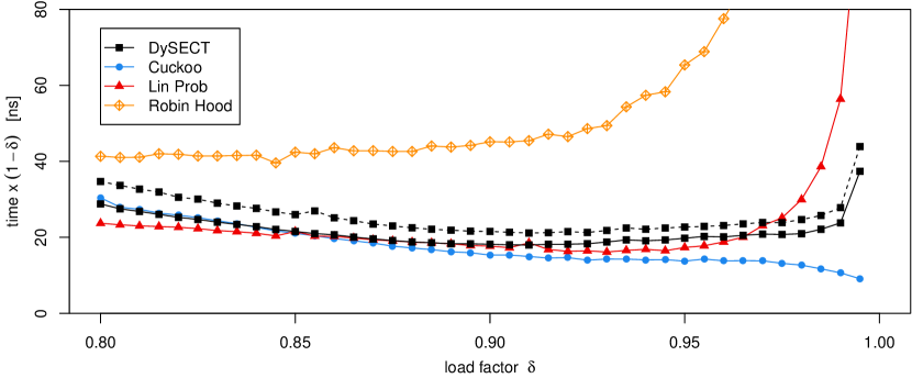
Figure 2: Insertions into a Static Table. Here we show the influence from the load factor, on the performance of insertions. To make insertion time more readable, we normalize it with $t_{op}\cdot(1-\delta)$.

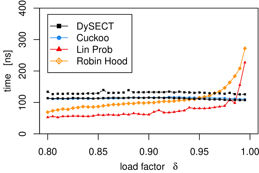
Figure 3: Performance of Successful Finds. DySECT’s find performance is independent from the load factor.

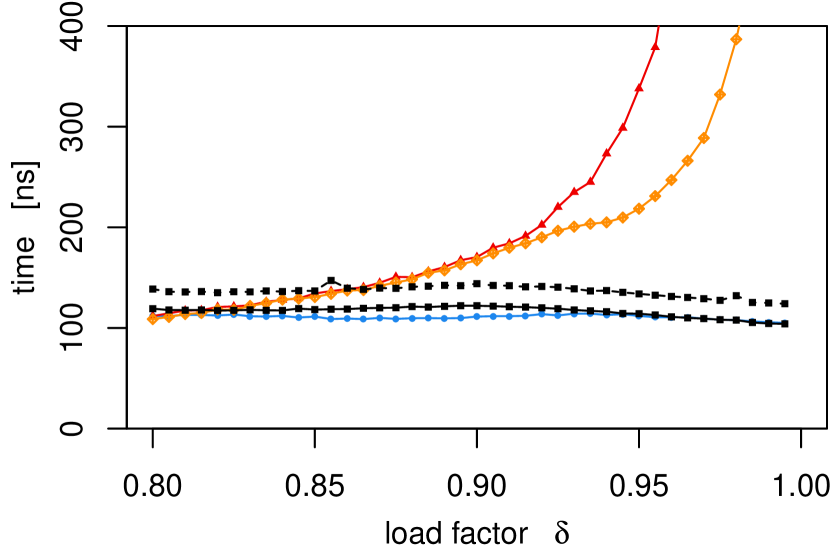
Figure 4: Performance of Unsuccessful Finds. DySECT’s find performance is independent from the operations success.

The following test was performed by initializing a table with $m\approx 25\,000\,000$ cells (non-growing). Then elements are inserted until there is a failing insertion. At different stages, we measure the running time of new insertion (Figure 2), and find (Figure 3 and 4) operations (averaged over 1000 operations). Finds are measured using either randomly selected elements from within the table (successful), or by searching random elements from the whole key space (unsuccessful). We omit testing multi table variants of the competitor tables. They are not suitable for this test since forcing a static size limits the possibility to react to size imbalances between subtables (in the absence of displacements).

As to be expected, the insertion performance of depends highly on the fill degree of the table. Therefore, we show it normalized with $\frac{1}{1-\delta}$ which is the expected number of fully random probes to find a free cell and thus a natural estimate for the running time. We see that – up to a certain point – the insertion time behaves proportional to $\frac{1}{1-\delta}$ for all tables. Close to the capacity limit of the table, the insertion time increases sharply. DySect has a smaller capacity limit than cuckoo due inhomogeneous table resolution (see Section 4.4).

Figure 3 and 4 show the performance of find operations. Linear probing performs relatively well on successful find operations, up to a fill degree of over 95%. The reason for this is that many elements were inserted into the table when the table was still relatively empty. They have very short search distances, thus improving find performance. Successful find performance can still be an issue in applications. An element that is inserted when the table is already decently filled can have an extremely long search distance. This leads to a high running time variance on find operations. Unsuccessful finds perform really badly, since all cells until the next free cell have to be probed. Their performance is much more related to the filling degree of the hash table. Robin Hood hashing performs somewhat similar to linear probing. It worsens the successful find performance by moving previously inserted elements from their original position, in order to achieve better unsuccessful find performance on highly filled tables. Overall, Robin Hood hashing is objectively worse than both DySECT and classic cuckoo hashing. Cuckoo hashing and its variants like DySECT have guaranteed constant running times for all find operations – independent of their success and the table’s filling degree.

6.2 Influence of Fill Ratio (Dynamic Table Size)

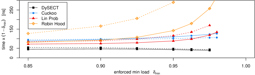
Figure 5: Insertions into a dynamic growing table enforcing a minimum load factor $\delta_{\min}$.

In this test 20 000 000 elements are inserted into an initially empty table. The table is initialized expecting 50 000 elements, thus growing is necessary to fit all elements. The tables are configured to guarantee a load factor of at least $\delta_{\min}$ at all times. Figure 5 shows the performance in relation to the load factor. Insertion times are computed as average of all 20 000 000 insertions. They are normalized similar to Figure 2 (divided by $\frac{1}{1-\delta_{\min}}$).

We see that DySECT performs by far the best even with less filled tables at 85% load. Here we achieve a speedup of 1.6 over the next best solution (299ns vs. linear probing 479ns). On denser instances with 97.5% load, we can increases these speedup to 2.7 (1580ns vs Cuckoo with subtables 4210ns). With growing load, we see the insertion times of our competitors degrade. The combination of long insertion times, and frequent growing phases slows them down. There are only few insertions between two growing phases. Making the amortization of each growing phase challenging since each growing phase has to move all elements. Any growing technique that uses a less cache efficient migration algorithm, would likely perform significantly worse. DySECT however remains close to $O(\frac{1}{1-\delta_{\min}})$ even for fill degrees up to 97.5$\%$. This is possible, because only very few elements are actually touched during each subtable migration ($\approx\frac{n}{T}$).

We also measured the performance of find operations on the created tables, they are similar to the performance on the static table in Section 6.1 (see Figure 3 and 4), therefore, we omit displaying them for space reasons.

6.3 Word Count – a Practical use Case

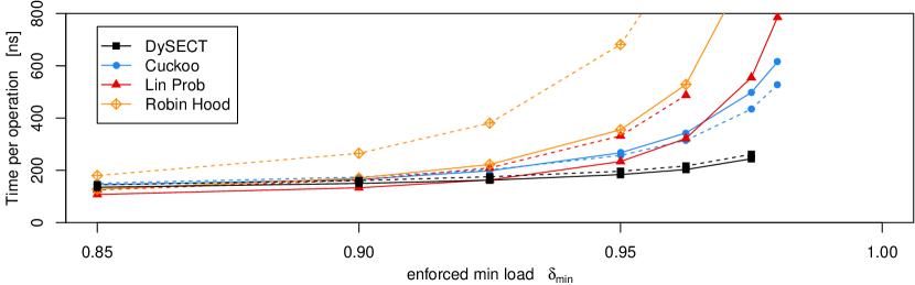
Figure 6: Word Count Benchmark. The benchmark behaves like a mix of insert and find operations. DySECT’s performance is nearly independent form the load factor.

Word count and other aggregation algorithms are some of the most common use cases for hash tables. Data is aggregated according to its key, which in our case is a hash of the contained word. This is a common application, in which static hash tables can never be space efficient, since the final size of the hash table is usually unknown. Here we use the first block of the CommonCrawl dataset (commoncrawl.org/the-data/get-started) and compute a word count of the contained words, using our hash tables. The chosen block has 4.2GB and contains around 240 000 000 words, with around 20 000 000 unique words. For the test, we hash each word to a 64 bit key and insert it together with a counter. Subsequent accesses to the same word increase this counter. Similar to the growing benchmark, we start with an empty table initialized for 50 000 elements.

The performance results can be seen in Figure 6. We do not use any normalization since each word is repeated 12 times (on average). This means that most operations will actually behave more like successful find operations instead of inserting an element. When using our DySECT table, the running time seems to be nearly independent from the fill degree. We experience little to no slowdown until around 97%. The tables using full table migration however become very inefficient on high load degrees.

For high load factors, the performance closely resembles that of the insertion benchmark (Figure 5). This indicates that insert performance can dominate running times even in find intensive workloads. To confirm this insight, we conducted some experiments with mixed operations (insert and find; insert and erase). They showed, that on a hash table with $\delta_{\min}=0.95$ DySECT outperforms linear probing for any workload containing more than 5$\%$ insertions (see Section 6.4).

6.4 Mixed Workloads

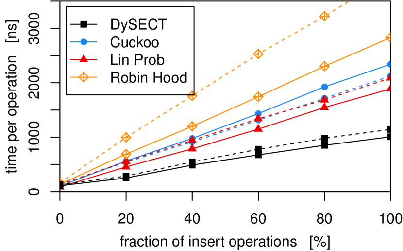
Figure 7: Workload combining insertions with finds.

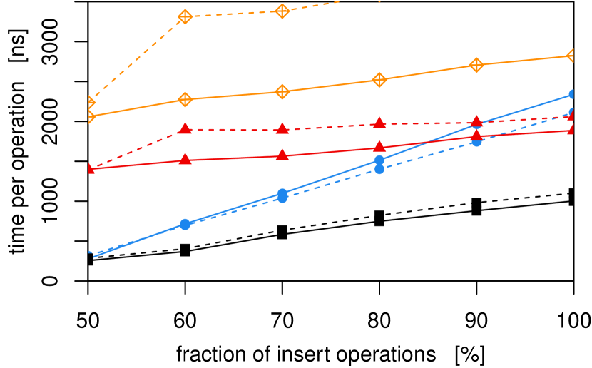
Figure 8: Workloads combining insertions with erase.

In this test, we show how the hash tables behave under mixed workloads. For this test we fixed the minimum load factor to $\delta=0.95$. The test starts with a filled table containing 15 000 000 elements (95% filled). On this table we perform 10 000 000 operations mixed between insert and find/erase operations.

As one might expect, the running time of a mixed work load can be estimated with a linear combination of the used operations.

In the insert/find benchmark (Figure 7), DySECT outperforms all other hash tables. This shows that fast insertions are important even in find intensive workloads. This is even more accentuated by the fact that all performed finds are successful finds which have usually better performance on hash tables using linear probing The measurements with deletions (Figure 8) show that deletions in linear probing tables are significantly slower than those in cuckoo tables. This makes sense, since linear probing tables have to move elements, to fix their invariants while cuckoo tables have guaranteed constant deletions.

6.5 Investigating Maximum Load Bounds

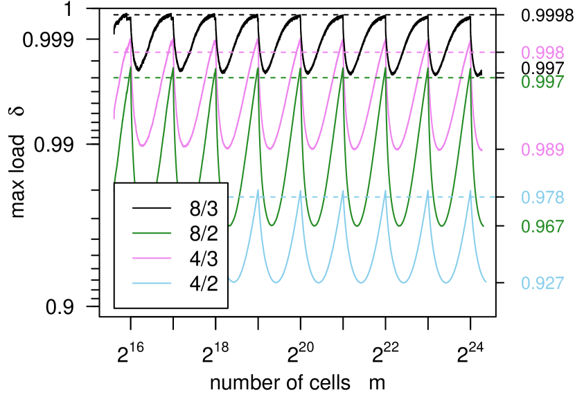
Figure 9: Maximum load bounds for different parameterizations ($B/H$) over a varying table size. Cuckoo’s bound is indicated by a dashed line.

We designed the following experiment, to give an indication for the theoretical load bounds DySECT is able to support. To do this, we configured DySECT to grow only if there is an unsuccessful insertion – in our other tests the table grows in anticipation once the size-constraint allows it. To get even closer to the theoretical limits, we use $T=4096$ subtables such that each grow has a smaller relative grow factor. Additionally we increase the number of probes used to find a successful displacement path to 16384 probes (from 1024).

We test different combinations of bucket size ($B$) and number of hash functions ($H$). The test consists of inserting 20 000 000 elements into a previously empty table initialized with 50 000 cells. Whenever the table has to grow we note its effective load (during the migration). The maximum load bound depends on the number of large subtables. Therefore, we show the achieved load factors over the table capacity ($m$). To give a perspective, of static table performance we show dashed lines with the performance of a cuckoo hash table. We measured cuckoo’s performance by initializing a table with 20 000 000 cells and filling it until there was an error (using the same search distance of 16384).

Figure 9 clearly shows the cyclical nature of DySECT’s maximum load bound. The table can be filled the most, when its capacity is close to a power of two. Then, all subtables have the same size and the table behaves similar to a static cuckoo table of the. On some sizes DySECT even seems to outperform cuckoo hashing. We are not sure why this is the case. We suspect that the bound measured for cuckoo hashing is not tight (cuckoo hashing bounds are only measured on one table size). This effect does not appear for the $8/3$ parameterization that we use throughout the paper.

Both parameterizations that are using only two hash functions ($8/2$ and $4/2$) have a higher dependency on the table size. The reason for this is that additional hash functions help to reduce the imbalance introduced by varied subtable resolution described in Section 4.4. Overall, we reach load bounds that are close to those of static cuckoo hashing.

7 Conclusion

We have shown that dynamically growing hash tables can be implemented to always consume space close to the lower bound. We find it surprising that even our simple solutions based on linear probing seem to be new. DySECT is a sophisticated solution that exploits the flexibility offered by bucket cuckoo hashing to significantly decrease the number of object migrations over more straightforward approaches. When very high space efficiency is desired, it is up to 2.7 times better than simple solutions.

For future work, a theoretical analysis of DySECT looks interesting. We expect that techniques previously used to analyze bucket cuckoo hashing will be applicable in principle. However, the already very complex calculations have to be generalized to take all possible ratios of small versus large subtables into account. Even for the static case and classical bucket cuckoo hashing, it is a fascinating open question whether the observed proportionality of insertion time to $1/(1-\delta)$ can be proven. Previous results on insertion time show much more conservative bounds [8, 9, 10, 7].

On the practical side, DySECT looks interesting for concurrent hashing [15, 18] since it grows only small parts of the table at a time.

Appendix A Parameterization of DySECT

In this section, we show additional measurements, using the experiment described in Section 6.2. We insert 20 000 000 elements into a previously empty table – using a dynamic table size. We show the measurements for different parameterizations of DySECT and Cuckoo Tables. First we show different combinations for $B$ and $H$, here we also show their find performance. Then we show different displacement techniques using ($B=8$ and $H=3$). For random walk displacements we test an optimistic, and a pessimistic variant.

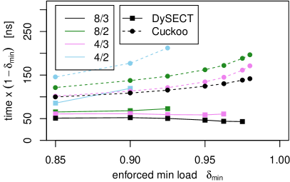
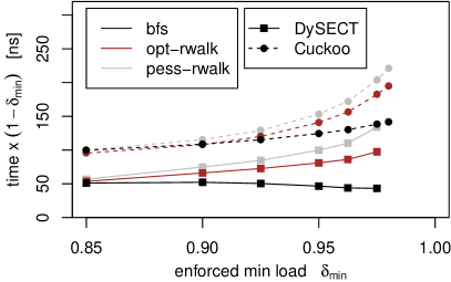
Figure 10: Insertions with different $B/H$ Parameterizations (left), and different Displacement techniques (using 8/3right). For each displacement, we perform up to 1024 probes for an empty bucket. Measurements end when errors occur.

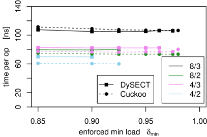
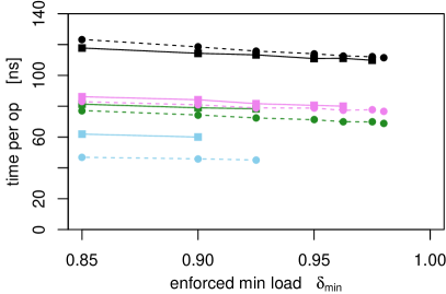
Figure 11: Finds with different $B/H$ Parameterizations (successful left, unsuccessfulright). Solid lines represents DySECT. Dashed lines represent bucket cuckoo hashing.

The measurements show, that the chosen parameterization in Section 4.5 has the best maximum fill bounds and the best insert performance. Both 4/3 and 8/2 might achieve better performance on sparser tables, with find heavy workloads.

References

- [1] Yuriy Arbitman, Moni Naor, and Gil Segev. De-amortized cuckoo hashing: Provable worst-case performance and experimental results. In International Conference on Automata, Languages and Programming (ICALP), number 5555 in LNCS, pages 107–118. Springer, 2009.
- [2] Pedro Celis, Per-Ake Larson, and J. Ian Munro. Robin hood hashing. In 26th Symposium on Foundations of Computer Science (FOCS), pages 281–288, Oct 1985.
- [3] Luc Devroye and Pat Morin. Cuckoo hashing: Further analysis. Information Processing Letters, 86(4):215 – 219, 2003.
- [4] Martin Dietzfelbinger, Andreas Goerdt, Michael Mitzenmacher, Andrea Montanari, Rasmus Pagh, and Michael Rink. Tight thresholds for cuckoo hashing via XORSAT. In 27th International Conference on Automata, Languages and Programming (ICALP), pages 213–225, 2010.
- [5] Martin Dietzfelbinger, Anna Karlin, Kurt Mehlhorn, Friedhelm Meyer auf der Heide, Hans Rohnert, and Robert E. Tarjan. Dynamic perfect hashing: Upper and lower bounds. SIAM Journal on Computing, 23(4):738–761, 1994.
- [6] Martin Dietzfelbinger, Michael Mitzenmacher, and Michael Rink. Cuckoo hashing with pages. In 19th European Symposium on Algorithms (ESA), number 6942 in LNCS, pages 615–627. Springer, 2011.
- [7] Martin Dietzfelbinger and Christoph Weidling. Balanced allocation and dictionaries with tightly packed constant size bins. Theoretical Computer Science, 380(1):47–68, 2007.
- [8] Dimitris Fotakis, Rasmus Pagh, Peter Sanders, and Paul Spirakis. Space efficient hash tables with worst case constant access time. Theory of Computing Systems, 38(2):229–248, 2005.
- [9] Nikolaos Fountoulakis, Konstantinos Panagiotou, and Angelika Steger. On the insertion time of cuckoo hashing. SIAM Journal on Computing, 42(6):2156–2181, 2013.
- [10] Alan Frieze, Páll Melsted, and Michael Mitzenmacher. An analysis of random-walk cuckoo hashing. SIAM Journal on Computing, 40(2):291–308, 2011.
- [11] Leo J. Guibas and Endre Szemeredi. The analysis of double hashing. Journal of Computer and System Sciences, 16(2):226–274, 1978.
- [12] Adam Kirsch and Michael Mitzenmacher. Less hashing, same performance: Building a better bloom filter. In Yossi Azar and Thomas Erlebach, editors, 14th European Symposium on Algorithms (ESA), number 4168 in LNCS, pages 456–467. Springer, 2006.
- [13] Adam Kirsch and Michael Mitzenmacher. Using a queue to de-amortize cuckoo hashing in hardware. In 45th Annual Allerton Conference on Communication, Control, and Computing, volume 75, 2007.
- [14] Donald E. Knuth. The Art of Computer Programming, Volume 3: (2nd Ed.) Sorting and Searching. Addison Wesley Longman Publishing Co., Inc., Redwood City, CA, USA, 1998.
- [15] Xiaozhou Li, David G. Andersen, Michael Kaminsky, and Michael J. Freedman. Algorithmic improvements for fast concurrent cuckoo hashing. In 9th European Conference on Computer Systems, EuroSys ’14, pages 27:1–27:14. ACM, 2014.
- [16] M. Mitzenmacher. The power of two choices in randomized load balancing. IEEE Transactions on Parallel and Distributed Systems, 12(10):1094–1104, Oct 2001.
- [17] Michael Mitzenmacher. Some open questions related to cuckoo hashing. In Amos Fiat and Peter Sanders, editors, 17th European Symposium on Algorithms (ESA), volume 5757 of LNCS, pages 1–10. Springer, 2009.
- [18] N. Nguyen and P. Tsigas. Lock-free cuckoo hashing. In 2014 IEEE 34th International Conference on Distributed Computing Systems (ICDCS), pages 627–636, June 2014.
- [19] Rasmus Pagh and Flemming Friche Rodler. Cuckoo hashing. Journal of Algorithms, 51(2):122–144, 2004.