Abstract

We show that the decay rates of the Higgs boson to a pseudoscalar quarkonium and a pair of leptons, $h\to P\ell^{+}\ell^{-}$ ($P\in\{\eta_{c},\eta_{b}\}$), can be substantially enhanced in a scenario with two Higgs doublets with a softly broken $\mathbb{Z}_{2}$ symmetry (2HDM) when the CP-odd Higgs $A$ is light, i.e. $m_{A}\lesssim m_{h}$. Depending on the type of 2HDM the enhancement of ${\mathcal{B}}(h\to\eta_{c,b}\tau^{+}\tau^{-})$ with respect to its Standard Model value can be an order of magnitude larger, i.e. $\mathcal{O}(10^{-6}\div 10^{-5})$. The decays $h\to P\ell^{+}\ell^{-}$ could therefore provide an efficient channel to investigate the presence of a light CP-odd Higgs $A$ and help to disentangle among various 2HDM scenarios.

1 Introduction

One of the minimal extensions of the Standard Model consists in enlarging the Higgs sector and, instead of one doublet of scalar fields, introducing an additional Higgs doublet, which comes under the generic name of Two Higgs Doublet Model (2HDM) [1]. With a peculiar choice of Yukawa couplings, 2HDM is embedded in the minimal supersymmetric extension of the Standard Model (MSSM) which made it particularly popular in phenomenological applications of low energy supersymmetry. The fact that the mass of observed Higgs boson was found to be consistent with the Standard Model expectations made MSSM less compelling but the 2HDM remains a convenient framework to study the extensions of the Higgs sector in view of the current experimental searches.

Despite its minimalism 2HDM has a rich structure. Besides the usual Higgs state $h$, there is an extra CP-even scalar ($H$) and two additional states of which one is a charged scalar boson ($H^{\pm}$) and another a CP-odd state ($A$). The state observed at LHC is identified with $h$ [2], or $H$ [3] which is otherwise expected to be heavier than $h$. A fact that the measured rates of the tree level weak decays of leptons and mesons are consistent with the Standard Model predictions is a hint that the charged Higgs is heavy too, also confirmed by the direct searches [4]. The CP-odd Higgs boson, instead, remains unconstrained explicitly. It is often assumed that its mass is larger than that of the observed Higgs, $m_{A}>m_{h}$. This, however, is just an assumption which should be tested experimentally. Several proposals to look for a light CP-odd Higgs were made in the past [5, 6, 7, 8]. In this paper we propose to study decays of Higgs to the pseudoscalar heavy quarkonia ($P$), $h\to P\ell^{+}\ell^{-}$, ($P\in\{\eta_{c},\eta_{b}\}$) processes in which the CP-odd Higgs can contribute at the tree level and make a significant enhancement of various decay rates. The level of such an enhancement is related to the structure of the Yukawa couplings and to the mass of the $A$-state. As we shall see in the following, we find that ${\mathcal{B}}(h\to\eta_{c,b}\tau^{+}\tau^{-})$ can be enhanced by an order of magnitude with respect to its Standard Model value, which is why we find it interesting and worth studying in experiments.

Studies of the Higgs boson to quarkonia attracted quite a bit of attention: Radiative decay $h\to J/\psi\gamma$ could be used to probe the Yukawa coupling $hc\bar{c}$, a possibility which is compromised in the case of $b$-quark quarkonia ($\Upsilon(nS)$) due to cancellation of two contributions to the decay amplitude [9]. A possibility to study $h\to PZ$ and $h\to VZ$ (where $V$ and $P$ stand for the vector and pseudoscalar quarkonium states, respectively) was elaborated in Refs. [10, 11]. Finally, a possibility to search for the effects of lepton flavour violation via $h\to V\ell_{1}\ell_{2}$ has been proposed in Ref. [12].

The remainder of this paper is organized as follows: In Sec. 2 we derive the expressions for ${\mathcal{B}}(h\to PZ)$ and ${\mathcal{B}}(h\to P\ell^{+}\ell^{-})$ both in the Standard Model and in 2HDM with a light CP-odd Higgs state. In Sec. 3 we scan the parameter space of 2HDM with a softly broken $\mathbb{Z}_{2}$ symmetry. The results of our scan are used in Sec. 4 where we test the sensitivity of ${\mathcal{B}}(h\to\eta_{c,b}\ell^{+}\ell^{-})$ on the presence of a light CP-odd Higgs state. We summarize our findings and briefly conclude in Sec. 5.

2 Expressions for ${\mathcal{B}}(h\to PZ)$ and ${\mathcal{B}}(h\to P\ell^{+}\ell^{-})$

In this Section we provide the expressions for ${\mathcal{B}}(h\to PZ)$ and ${\mathcal{B}}(h\to P\ell^{+}\ell^{-})$ both in the Standard Model (SM) and in the generic 2HDM scenario. To do so we need to specify the notation. By $P$ we denote the pseudoscalar quarkonium carrying momentum $k$, while $Z$ flies with momentum $p_{Z}$. The dilepton invariant mass squared in the $P\ell^{+}\ell^{-}$ final state is considered as $q^{2}=(p_{\ell}+p_{\bar{\ell}})^{2}$, with $p_{\ell,\bar{\ell}}$ being the momentum of the outgoing leptons.

2.1 ${\mathcal{B}}(h\to PZ)$

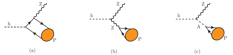
Figure 1: Diagrams contributing $h\to PZ$ decay.

In the SM the decay $h\to PZ$ occurs via the diagrams (a) and (b) shown in Fig. 1. The dominant (“indirect”) contribution comes from $h\to ZZ^{\ast}\to ZP$ (Fig. 1b) which is much larger than the direct one, $h\to Z\bar{q}q\to ZP$ (Fig. 1a). In a 2HDM an additional significant contribution arises from $h\to ZA^{\ast}\to ZP$ (Fig. 1c), which can be large if the CP-odd Higgs is light and the corresponding couplings to fermions are non-negligible. The decay amplitude then can be written as,

$$\mathcal{M}(h\to PZ)=\frac{g}{v\cos\theta_{W}}\ \left(k\cdot\varepsilon_{Z}^{\ast}\right)\ F^{\mathrm{PZ}},$$ (1)

with

$$F^{\mathrm{PZ}}\approx{m_{Z}^{2}\over m_{Z}^{2}-m_{P}^{2}}f_{P}g_{A}^{q}-{f_{P}v\over m_{A}^{2}-m_{P}^{2}+im_{A}\Gamma_{A}}{m_{P}^{2}\over 2m_{q}}{m_{q}\over v}\xi_{A}^{q}\cos(\beta-\alpha),$$ (2)

where we displayed only the dominant SM contribution and the one arising from the CP-odd Higgs in the 2HDM. In the above formula $g_{A}^{q}=T_{q}^{3}$, $\xi_{A}^{q}$ is a coupling of the $q\bar{q}$-par to the CP-odd Higgs state which will be defined below [cf. Eq. (3)], and we have used the standard definition of the decay constant $f_{P}$, namely,

$$\langle P(k)|\bar{q}\gamma^{\mu}\gamma_{5}q|0\rangle=-if_{P}k_{\mu},\qquad\langle P(k)|\bar{q}\gamma^{5}q|0\rangle=-if_{P}{m_{P}^{2}\over 2m_{q}},$$ (3)

where $q=c$ or $b$, for $P=\eta_{c}$ or $\eta_{b}$, respectively. We should emphasize that owing to the fact that $\eta_{c,b}$ is a flavor singlet and therefore it can also couple to $(\alpha_{s}/4\pi)F_{\mu\nu}\widetilde{F}^{\mu\nu}$, with $F$ ($\widetilde{F}$) being the (dual) QCD field strength tensor. While such a term is important for the light quark flavor singlets ($\pi^{0}$, $\eta$, $\eta^{\prime}$), it is expected to be very small for the case of heavy quarkonia, which is why it will be neglected in the following.  With the above definitions, the decay rate then reads,

$$\Gamma(h\to PZ)={\lambda^{3/2}(m_{h},m_{P},m_{Z})\over 16\pi v^{4}m_{h}^{3}}|F^{\mathrm{PZ}}|^{2}\,,$$ (4)

where $\lambda(a,b,c)=[a^{2}-(b+c)^{2}][a^{2}-(b-c)^{2}]$. Notice that in the above amplitude we kept the width of the CP-odd Higgs boson different from zero. In the limit in which $\Gamma_{A}/m_{A}\ll 1$, one can work in the narrow width approximation, which amounts to replacing

$${1\over(q-m_{X})^{2}+m_{X}^{2}\Gamma_{X}^{2}}\to\delta(q^{2}-m_{X}^{2}){\pi\over m_{X}\Gamma_{X}}\,.$$ (5)

This approximation is adopted throughout this paper both for $X=Z$ and $X=A$. We emphasize that, for clarity, we disregarded the direct contributions to the amplitude because they are numerically much smaller and, since the corresponding expression is more complicated, we decided to relegate it to the Appendix.  To get the branching fraction in a 2HDM setup, one should be particularly careful with the width of the Higgs boson $\Gamma_{h}$ which should not be much larger than its SM value, e.g. $\Gamma_{h}/\Gamma_{h}^{\mathrm{SM}}\lesssim 1.4$, a condition that provides a particularly stringent bound on the coupling of $h$ to two light CP-odd Higgses in the situation in which $m_{A}\leq m_{h}/2$. To be more specific, from the general 2HDM potential, we can read off the term corresponding to the trilinear interaction, namely,

$$\mathcal{L}_{\mathrm{2HDM}}\supset\frac{v}{2!}\lambda_{hAA}\ hAA,$$ (6)

where $v\approx 246$ GeV, and the coupling

$$\lambda_{hAA}=\frac{1}{2v^{2}\sin(2\beta)} \biggl{\{}m_{h}^{2}\left[\cos(\alpha-3\beta)+3\cos(\alpha+\beta)\right]\biggr{.}$$

$$\biggl{.}\quad+4m_{A}^{2}\sin(2\beta)\sin(\beta-\alpha)-4M^{2}\cos(\alpha+\beta)\biggr{\}}\,,$$ (7)

with $\alpha,\leavevmode\nobreak\ \beta$ and $M^{2}$ explicitly defined in Sec. 3. The expression for the decay width reads:

$$\Gamma(h\to AA)={|\lambda_{hAA}|^{2}\over 32\pi}\frac{v^{2}}{m_{h}}\sqrt{1-\frac{4m_{A}^{2}}{m_{h}^{2}}}\,.$$ (8)

Besides $h\to AA$, if opened, the channel $h\to ZA$ can give significant contribution to the width $\Gamma_{h}$. The decay width of this particular channel is given by

$$\Gamma(h\to ZA)={1\over 16\pi}\frac{\cos^{2}(\beta-\alpha)}{m_{h}^{3}v^{2}}\lambda^{3/2}(m_{h},m_{Z},m_{A})\,.$$ (9)

2.2 ${\mathcal{B}}(h\to P\ell^{+}\ell^{-})$

In the Standard Model the situation with $h\to P\ell^{+}\ell^{-}$ is similar to the one discussed in the case of $h\to PZ$. The dominant contribution comes from the diagram Fig. 2c

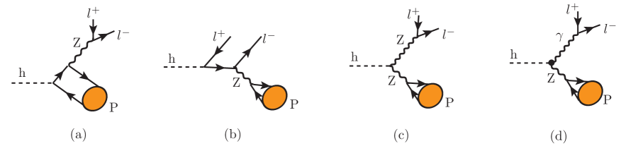
Figure 2: Diagrams relevant to $h\to P\ell^{+}\ell^{-}$ decay in the Standard Model. The full dot in the diagram (d) indicates that the vertex is loop-induced. Its contribution to the decay rate is nevertheless zero.

which reads

$$\mathcal{M}(h\to P\ell^{+}\ell^{-})^{\mathrm{2c}}= -\frac{1}{4}\left(\frac{g}{\cos\theta_{W}}\right)^{3}m_{Z}\ {g_{A}^{q}f_{P}\over(q^{2}-m_{Z}^{2})\ (k^{2}-m_{Z}^{2})}\left(-g^{\alpha}_{\mu}+{q^{\mu}q_{\alpha}\over m_{Z}^{2}}\right)$$

$$\left(-g^{\nu\alpha}+{k^{\nu}k^{\alpha}\over m_{Z}^{2}}\right)\ k_{\nu}\ \bar{u}_{\ell}\gamma^{\mu}(g_{V}^{\ell}-g_{A}^{\ell}\gamma_{5})v_{\ell}\,.$$ (10)

The full expression, which includes all contributions depicted in Fig. 2, is given in Appendix of the present paper. We note, however, that the contribution of the diagram in Fig. 2d vanishes in the decay rate.

Diagrams arising in the 2HDM setup are shown in Fig. 3, of which the first two are numerically much less significant than the remaining three. The contributions of those latter (dominant) diagrams to the decay amplitude read:

$$\mathcal{M}(h\to P\ell^{+}\ell^{-})^{\mathrm{3c}}= -\left(\frac{g}{2\cos\theta_{W}}\right)^{2}\frac{m_{q}\xi^{q}_{A}}{v}\frac{m_{P}^{2}f_{P}}{2m_{q}}\ {\cos(\beta-\alpha)\over(q^{2}-m_{Z}^{2})\ (k^{2}-m_{A}^{2})}$$

$$\left(-g_{\mu\nu}+{q_{\mu}q_{\nu}\over m_{Z}^{2}}\right)\ (k+p)^{\mu}\ \bar{u}_{\ell}\gamma^{\nu}(g_{V}^{\ell}-g_{A}^{\ell}\gamma_{5})v_{\ell}\,,$$ (11)

$$\mathcal{M}(h\to P\ell^{+}\ell^{-})^{\mathrm{3d}}= \left(\frac{g}{2\cos\theta_{W}}\right)^{2}\frac{m_{\ell}\xi^{\ell}_{A}}{v}{g_{A}^{q}f_{P}\cos(\beta-\alpha)\over(q^{2}-m_{A}^{2})\ (k^{2}-m_{Z}^{2})}$$

$$\left(-g_{\mu\nu}+{k_{\mu}k_{\nu}\over m_{Z}^{2}}\right)\ (q+p)^{\mu}k^{\nu}\ \bar{u}_{\ell}\gamma_{5}v_{\ell}\,,$$ (12)

$$\mathcal{M}(h\to P\ell^{+}\ell^{-})^{\mathrm{3e}}=- \lambda_{hAA}v\ \frac{m_{q}\xi^{q}_{A}}{v}\frac{m_{\ell}\xi^{\ell}_{A}}{v}\frac{m_{P}^{2}f_{P}}{2m_{q}}{1\over(q^{2}-m_{A}^{2})\ (k^{2}-m_{A}^{2})}\bar{u}_{\ell}\gamma_{5}v_{\ell}\,.$$ (13)

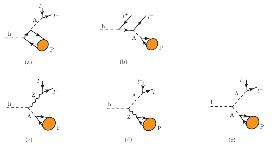
Figure 3: Contributions to the $h\to P\ell^{+}\ell^{-}$ decay amplitude in a 2HDM scenario.

To a very good approximation the decay rate can be written as

$$\Gamma(h\to P\ell^{+}\ell^{-})\simeq\Gamma(h\to PZ^{\ast}\to P\ell^{+}\ell^{-})+\Gamma(h\to PA^{\ast}\to P\ell^{+}\ell^{-}).$$ (14)

We checked that the interference terms are indeed very small and the above formula is useful for the phenomenology we are interested in. For the explicit expressions of the separate rates in Eq. (14) we obtain,

$$\Gamma(h\to PZ^{\ast}\to P\ell^{+}\ell^{-})= {f_{P}^{2}m_{Z}^{3}\over 384\pi^{2}\Gamma_{Z}m_{h}^{3}v^{6}}\bigl{[}\cos^{2}(2\theta_{W})+4\sin^{4}\theta_{W}\bigr{]}$$

$$\left(g_{A}^{q}-{\xi_{A}^{q}m_{P}^{2}\cos(\beta-\alpha)\over 2(m_{A}^{2}-m_{P}^{2})}\right)^{2}\lambda^{3/2}(m_{h},m_{P},m_{Z}),$$ (15)

$$\Gamma(h\to PA^{\ast}\to P\ell^{+}\ell^{-})= {f_{P}^{2}m_{A}\over 512\pi^{2}\Gamma_{A}m_{h}^{3}v^{2}}\left(\frac{m_{\ell}\xi_{A}^{\ell}}{v}\right)^{2}\biggl{[}\lambda_{hAA}\frac{m_{P}^{2}}{m_{A}^{2}-m_{P}^{2}}\frac{\xi_{A}^{q}}{v}v^{2}\biggr{.}$$

$$\biggl{.}+2\cos(\beta-\alpha){g_{A}^{q}\over v}(m_{h}^{2}-m_{A}^{2})\biggr{]}^{2}\ \lambda^{1/2}(m_{h},m_{P},m_{A}).$$ (16)

In the above formulas $g_{V}^{f}=T_{f}^{3}-2Q_{f}\sin^{2}\theta_{W}$, $g_{A}^{f}=T_{f}^{3}$, and we neglected the additive terms $\propto m_{\ell}^{2}/m_{Z}^{2}$. We emphasize once again that the above expression for $\Gamma(h\to P\ell^{+}\ell^{-})$ should be viewed as a very good approximation, whereas the full expressions are provided in the Appendix of the present paper.

Finally, since the above formulas require the knowledge of the width of $A$, we give that expression too, in which we include $\Gamma_{A}=\Gamma(A\to f\bar{f})+\Gamma(A\to\gamma\gamma)$, which are given by

$$\Gamma(A\to f\bar{f}) =\theta(m_{A}-2m_{f})|\xi_{A}^{f}|^{2}\,{N_{c}m_{f}^{2}\over 8\pi v^{2}}\,m_{A}\,\sqrt{1-\frac{4m_{f}^{2}}{m_{A}^{2}}}\,,$$

$$\Gamma(A\to\gamma\gamma) =\frac{\alpha_{\mathrm{em}}^{2}}{16\pi^{3}v^{2}}m_{A}^{3}\left|\sum_{f}\xi_{A}^{f}\,N_{c}\,Q_{f}^{2}\,x_{f}\,F_{\gamma\gamma}(x_{f})\right|^{2}\,,$$ (17)

where $N_{c}=3$ for quarks and $N_{c}=1$ for leptons, the electric charge for leptons, up-type and down-type quarks is $Q_{\ell}=-1$, $Q_{u}=2/3$, $Q_{d}=-1/3$, respectively, and $f$ runs over all available quark and lepton flavors. In the above expression we used the notation $x_{f}=m_{f}^{2}/m_{A}^{2}$, and the loop function reads

$$F_{\gamma\gamma}(x)=\left\{\begin{array}[]{lr}\frac{1}{2}\left(i\pi+\log\left[\displaystyle{1+\sqrt{1-4x}\over 1-\sqrt{1-4x}}\right]\right)^{2},&\text{for }x<1/4\\ -2\arcsin^{2}\left(\displaystyle{1\over 2\sqrt{x}}\right),&\text{otherwise }\end{array}\right..$$ (18)

Notice that $\Gamma(A\to\gamma\gamma)\ll\Gamma(A\to f\bar{f})$ and our conclusion would remain the same even if we neglected $\Gamma(A\to\gamma\gamma)$. For the same reason we neglect the $\Gamma(A\to gg)$ contribution to the full width of $A$.

3 Scanning the 2HDM parameter space

We consider a general CP-conserving 2HDM with a softly broken $\mathbb{Z}_{2}$ symmetry, described by the following potential:

$$V(\Phi_{1},\Phi_{2})=m_{11}^{2}\Phi_{1}^{\dagger}\Phi_{1} +m_{22}^{2}\Phi_{2}^{\dagger}\Phi_{2}+m_{12}^{2}(\Phi_{1}^{\dagger}\Phi_{2}+\Phi_{2}^{\dagger}\Phi_{1})+\dfrac{\lambda_{1}}{2}(\Phi_{1}^{\dagger}\Phi_{1})^{2}+\dfrac{\lambda_{2}}{2}(\Phi_{2}^{\dagger}\Phi_{2})^{2}$$

$$+\lambda_{3}\Phi_{1}^{\dagger}\Phi_{1}\Phi_{2}^{\dagger}\Phi_{2}+\lambda_{4}\Phi_{1}^{\dagger}\Phi_{2}\Phi_{2}^{\dagger}\Phi_{1}+\dfrac{\lambda_{5}}{2}\left[(\Phi_{1}^{\dagger}\Phi_{2})^{2}+(\Phi_{2}^{\dagger}\Phi_{1})^{2}\right],$$ (19)

where the term proportional to $m_{12}^{2}$ breaks the $\mathbb{Z}_{2}$ symmetry. In the above expression $\Phi_{a}$ ($a=1,2$) stand for a scalar doublet

$$\Phi_{a}(x)=\begin{pmatrix}\phi_{a}^{+}(x)\\ \frac{1}{\sqrt{2}}(v_{a}+\rho_{a}(x)+i\eta_{a}(x))\end{pmatrix},$$ (20)

where $v_{1,2}$ are the vacuum expectation values related to $v^{\mathrm{SM}}=\sqrt{v_{1}^{2}+v_{2}^{2}}=246.22$ GeV [13]. Two of the above fields are Goldstone bosons ($G^{0}$, $G^{\pm}$), two are massive CP-even states ($h$, $H$), one CP-odd ($A$), and one charged Higgs ($H^{\pm}$). These fields are related to the ones given in Eq. (20) via

$$\begin{pmatrix}\phi_{1}^{+}\\ \phi_{2}^{+}\end{pmatrix} =\begin{pmatrix}\cos\beta&-\sin\beta\\ \sin\beta&\cos\beta\end{pmatrix}\begin{pmatrix}G^{+}\\ H^{+}\end{pmatrix},\qquad\begin{pmatrix}\eta_{1}\\ \eta_{2}\end{pmatrix}=\begin{pmatrix}\cos\beta&-\sin\beta\\ \sin\beta&\cos\beta\end{pmatrix}\begin{pmatrix}G^{0}\\ A\end{pmatrix},$$

$$\begin{pmatrix}\rho_{1}\\ \rho_{2}\end{pmatrix} =\begin{pmatrix}\cos\alpha&-\sin\alpha\\ \sin\alpha&\cos\alpha\end{pmatrix}\begin{pmatrix}H\\ h\end{pmatrix},$$ (21)

where the mixing angles $\alpha$ and $\beta$ satisfy

$$\tan\beta=\frac{v_{2}}{v_{1}},\qquad\tan 2\alpha=\dfrac{2(-m_{12}^{2}+\lambda_{345}v_{1}v_{2})}{m_{12}^{2}(v_{2}/v_{1}-v_{1}/v_{2})+\lambda_{1}v_{1}^{2}-\lambda_{2}v_{2}^{2}},$$ (22)

with $\lambda_{345}\equiv\lambda_{3}+\lambda_{4}+\lambda_{5}$. The masses of the physical scalars can be written in terms of parameters which appear in the potential as

$$m_{H}^{2} =M^{2}\sin^{2}(\alpha-\beta)+\left(\lambda_{1}\cos^{2}\alpha\cos^{2}\beta+\lambda_{2}\sin^{2}\alpha\sin^{2}\beta+\frac{\lambda_{345}}{2}\sin 2\alpha\sin 2\beta\right)v^{2},$$

$$m_{h}^{2} =M^{2}\cos^{2}(\alpha-\beta)+\left(\lambda_{1}\sin^{2}\alpha\cos^{2}\beta+\lambda_{2}\cos^{2}\alpha\sin^{2}\beta-\frac{\lambda_{345}}{2}\sin 2\alpha\sin 2\beta\right)v^{2},$$

$$m_{A}^{2} =M^{2}-\lambda_{5}v^{2},$$

$$m_{H^{\pm}}^{2} =M^{2}-\frac{\lambda_{4}+\lambda_{5}}{2}v^{2},$$ (23)

where for shortness we use $M^{2}=m_{12}^{2}/(\sin\beta\cos\beta)$. As far as the Yukawa sector is concerned, the $\mathbb{Z}_{2}$ symmetry is imposed to prevent the flavor changing processes to appear at tree level [14] by enforcing each type of the right-handed fermion to couple to a single Higgs doublet. Four choices are then possible and they are called Type I, II, X and Z [1]. By writing the Yukawa Lagrangian as

$$\mathcal{L}_{Y}= -\dfrac{\sqrt{2}}{v}H^{+}\Big{\{}\bar{u}\leavevmode\nobreak\ [\zeta^{d}\,V_{\mathrm{CKM}}m_{d}P_{R}-\zeta^{u}\,m_{u}V_{\mathrm{CKM}}P_{L}]\leavevmode\nobreak\ d+\zeta^{\ell}\,\bar{\nu}m_{\ell}P_{R}\ell\Big{\}}$$

$$-\dfrac{1}{v}\sum_{f,\varphi_{i}^{0}\in\{h,H,A\}}\xi^{f}_{\varphi_{i}^{0}}\leavevmode\nobreak\ \varphi_{i}^{0}\,\Big{[}\bar{f}m_{f}P_{R}f\Big{]}+\mathrm{h.c.},$$ (24)

where a specific choice of parameters $\zeta^{f}$ corresponds to the above mentioned types of 2HDM, cf. Table 1. In the expression $u$, $d$ and $\ell$ stand for the up-type, down-type quark, and a lepton flavor respectively, and $f$ for a generic fermion. $V_{\mathrm{CKM}}$ is the Cabibbo–Kobayashi-Maskawa matrix, lepton mixing are neglected, and $P_{L,R}=(1\mp\gamma_{5})/2$. Furthermore, the couplings $\xi^{f}_{\varphi_{i}^{0}}$ are related to $\zeta^{f}$ as:

$$\xi_{h}^{f} =\sin(\beta-\alpha)+\cos(\beta-\alpha)\zeta^{f},$$

$$\xi_{H}^{f} =\cos(\beta-\alpha)-\sin(\beta-\alpha)\zeta^{f},$$

$$\xi_{A}^{u} =-i\zeta^{u},\qquad\xi_{A}^{d,\ell}=i\zeta^{d,\ell}.$$ (25)

Model	$\zeta^{d}$	$\zeta^{u}$	$\zeta^{\ell}$
Type I	$\cot\beta$	$\cot\beta$	$\cot\beta$
Type II	$-\tan\beta$	$\cot\beta$	$-\tan\beta$
Type X (lepton specific)	$\cot\beta$	$\cot\beta$	$-\tan\beta$
Type Z (flipped)	$-\tan\beta$	$\cot\beta$	$\cot\beta$

Table 1: Couplings $\zeta^{f}$ in various types of 2HDM.

Once we spelled out all the parameters of 2HDM we need to perform a scan of the parameters by taking into account the following general theory constraints:

• Stability of the scalar potential is ensured by the requirement that it is bounded from below, which is achieved if the quartic couplings satisfy [15]

  $$\lambda_{1,2}>0,\qquad\lambda_{3}>-(\lambda_{1}\lambda_{2})^{1/2},\qquad\lambda_{3}+\lambda_{4}-|\lambda_{5}|>-(\lambda_{1}\lambda_{2})^{1/2},$$ (26)

  while the stability of the electroweak vacuum requires

  $$m_{11}^{2}+\dfrac{\lambda_{1}v_{1}^{2}}{2}+\dfrac{\lambda_{3}v_{2}^{2}}{2} =\frac{v_{2}}{v_{1}}\left[m_{12}^{2}-(\lambda_{4}+\lambda_{5})\dfrac{v_{1}v_{2}}{2}\right],$$ (27)

  $$m_{22}^{2}+\dfrac{\lambda_{2}v_{2}^{2}}{2}+\dfrac{\lambda_{3}v_{1}^{2}}{2} =\frac{v_{1}}{v_{2}}\left[m_{12}^{2}-(\lambda_{4}+\lambda_{5})\dfrac{v_{1}v_{2}}{2}\right].$$ (28)

  In order for a minimum to be global, the parameters should also satisfy [16]:

  $$m_{12}^{2}\left(m_{11}^{2}-m_{22}^{2}\sqrt{\lambda_{1}/\lambda_{2}}\right)\left(\tan\beta-\sqrt[4]{\lambda_{1}/\lambda_{2}}\right)>0.$$ (29)

• Unitarity of the $S$-wave of the scalar scattering amplitudes gives rise to the following inequalities [17, 18]

  $$|a_{\pm}|,|b_{\pm}|,|c_{\pm}|,|f_{\pm}|,|e_{1,2}|,|f_{1}|,|p_{1}|<8\pi,$$ (30)

  where

  $$\begin{split}a_{\pm}&=\dfrac{3}{2}(\lambda_{1}+\lambda_{2})\pm\sqrt{\dfrac{9}{4}(\lambda_{1}-\lambda_{2})^{2}+(2\lambda_{3}+\lambda_{4})^{2}},\\ b_{\pm}&=\dfrac{1}{2}(\lambda_{1}+\lambda_{2})\pm\dfrac{1}{2}\sqrt{(\lambda_{1}-\lambda_{2})^{2}+4\lambda_{4}^{2}},\\ c_{\pm}&=\dfrac{1}{2}(\lambda_{1}+\lambda_{2})\pm\dfrac{1}{2}\sqrt{(\lambda_{1}-\lambda_{2})^{2}+4\lambda_{5}^{2}},\\ e_{1}&=\lambda_{3}+2\lambda_{4}-3\lambda_{5},\hskip 85.35826pte_{2}=\lambda_{3}-\lambda_{5},\\ f_{+}&=\lambda_{3}+2\lambda_{4}+3\lambda_{5},\hskip 82.51282ptf_{-}=\lambda_{3}+\lambda_{5},\\ f_{1}&=\lambda_{3}+\lambda_{4},\hskip 122.34692ptp_{1}=\lambda_{3}-\lambda_{4}.\end{split}$$ (31)

• Electroweak precision tests provide important constraint to the 2HDM parameters. We consider the expressions for the parameters $S$, $T$ and $U$ in 2HDM [19], and the values for $\Delta S$, $\Delta T$, $\Delta U$ given in Ref. [20],

  $$\begin{aligned} &\Delta S^{\rm SM}=0.05\pm 0.11,\\ &\Delta T^{\rm SM}=0.09\pm 0.13,\\ &\Delta U^{\rm SM}=0.01\pm 0.11,\\ \end{aligned}\qquad\qquad\mathrm{cov}=\left(\begin{array}[]{ccc}1&0.90&-0.59\\ 0.90&1&-0.83\\ -0.59&-0.83&1\end{array}\right),$$ (32)

  to $99\%$ C.L. Using $X=(\Delta S,\Delta T,\Delta U)$, $\sigma=(0.11,0.13,0.11)$, and $\sigma_{ij}^{2}\equiv\sigma_{i}\mathrm{cov}_{ij}\sigma_{j}$, we build

  $$\chi^{2}=\sum_{i,j}(X_{i}-X_{i}^{\rm SM})(\sigma^{2})_{ij}^{-1}(X_{j}-X_{j}^{\rm SM}).$$ (33)

  and choose the points which agree with the above numbers.

In our scan we identify the lightest CP-even state ($h$) with the SM-like scalar, observed at the LHC, with mass $m_{h}=125.09(24)$ GeV [13]. We assume ${\mathcal{B}}(h\to\mathrm{invisible})\leq 0.3$, and impose the near-alignment condition, $|\cos(\beta-\alpha)|\leq 0.3$, in order to ensure that $g_{hWW}$ and $g_{hZZ}$ remain consistent with the measured values and in agreement with the SM predictions [21] . The above-mentioned constraints are then imposed onto a set of randomly generated points in the intervals:

$$\begin{split}&\tan\beta\in(0.2,50),\qquad\hskip 42.67912pt\alpha\in\left(-\frac{\pi}{2},\frac{\pi}{2}\right),\qquad\hskip 28.45274pt\left|M^{2}\right|\leq(1\leavevmode\nobreak\ \mathrm{TeV})^{2},\\[6.00006pt] &m_{H^{\pm}}\in(m_{W},1\leavevmode\nobreak\ \mathrm{TeV}),\qquad m_{H}\in(m_{h},1\leavevmode\nobreak\ \mathrm{TeV}),\qquad m_{A}\in\left(20\ {\rm GeV},m_{h}\right).\end{split}$$ (34)

Due to correlation between $m_{A}$ and $m_{H^{\pm}}$, the fact that we choose to work with light CP-odd Higgs implies that the charged Higgs is bounded from above. We find $m_{H^{\pm}}\lesssim 700$ GeV, as shown in Fig. 4. In addition to the above constraints we also impose the bound arising from the comparison between theory predictions and the experimental results concerning the spectrum of $B\to X_{s}\gamma$ decay, which for the case of Type II and Type Z models amounts to a $3\sigma$ bound of $m_{H^{\pm}}\geq 439$ GeV [22]. Furthermore, the $3\sigma$ bounds coming from the exclusive $b\to s\mu^{+}\mu^{-}$ decay modes, discussed in Ref. [23], have also been included.

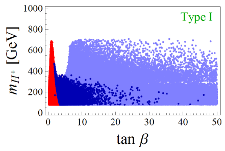
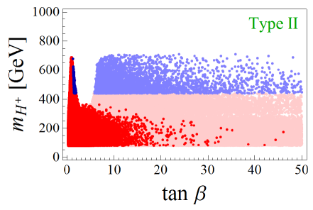
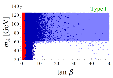
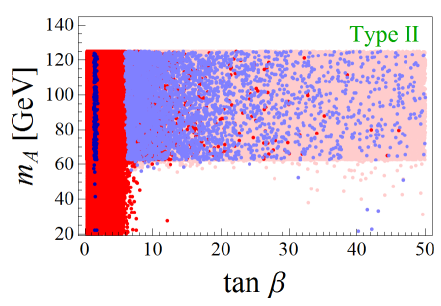
Figure 4: Results of the scan of parameters (34) after imposing constraints discussed in the text. Darker/lighter points correspond to the free/fine-tuned scan. Notice in particular that the red points are forbidden by the flavor bounds [22, 23].

It is important to mention that a scan of parameters consistent with the constraints listed above favors the moderate and small values of $\tan\beta\in(0.2,15]$. Larger values of $\tan\beta$ can be probed around the alignment limit as it can be seen from Eq. (3). For that reason, in addition to the free scan, we also perform a fine-tuned scan, i.e. with $m_{H}\approx|M|$. We combine both results and show them in Fig. 4 for Type I and Type II models. Similar results are obtained for Type X and Type Z. The lower bound on the charged Higgs, $m_{H^{\pm}}\geq 439$ GeV [22], eliminates many points in Type II and Type Z models. As it can be seen from Fig. 4, among the remaining points in the parameter space of the Type II model, the free scan prefers low $\tan\beta\approx 2$ values, while the large $\tan\beta$ values can only be accessed through the scan in the $m_{H}\approx|M|$ direction. The same observation applies to the Type Z model.

Notice also that one cannot simultaneously access $m_{A}<m_{h}/2$ and have large $\tan\beta$, except for the very fine tuned solutions. To see that we expand Eq. (2.1) around the alignment limit, $\delta=\cos(\alpha-\beta)\approx 0$, and obtain

$$\lambda_{hAA}=\frac{m_{h}^{2}+2m_{A}^{2}-2M^{2}}{v^{2}}+\frac{2(m_{h}^{2}-m_{H}^{2})}{v^{2}\tan 2\beta}\delta+\mathcal{O}(\delta^{2}).$$ (35)

To suppress $h\to\mathrm{invisible}$ in the perfect alignment limit, one needs $2M^{2}=m_{h}^{2}+2m_{A}^{2}$, which for the low $m_{A}$ gives $M^{2}\leq 3m_{h}^{2}/4\ll m_{H}^{2}$. Therefore, in order to get the large $\tan\beta$ values one needs $M\approx m_{H}$ which is in contradiction with the previous inequality.

4 Sensitivity of ${\mathcal{B}}(h\to PZ)$ and ${\mathcal{B}}(h\to P\ell^{+}\ell^{-})$ on the light CP-odd Higgs state

In this Section we use the results of the scan discussed above and evaluate

$$R^{Z}_{\eta_{cb}}={{\mathcal{B}}(h\to\eta_{cb}Z)^{\mathrm{2HDM}}\over{\mathcal{B}}(h\to\eta_{cb}Z)^{\mathrm{SM}}}\ ,$$

j $$R^{\tau\tau}_{\eta_{cb}}={{\mathcal{B}}(h\to\eta_{cb}\tau^{+}\tau^{-})^{\mathrm{2HDM}}\over{\mathcal{B}}(h\to\eta_{cb}\tau^{+}\tau^{-})^{\mathrm{SM}}}\ ,$$

j $$R^{\mu\mu}_{\eta_{cb}}={{\mathcal{B}}(h\to\eta_{cb}\mu^{+}\mu^{-})^{\mathrm{2HDM}}\over{\mathcal{B}}(h\to\eta_{cb}\mu^{+}\mu^{-})^{\mathrm{SM}}}\ ,$$ (36)

where $\eta_{cb}$ means either ${\eta_{c}}$ or $\eta_{b}$. Essential hadronic quantities needed to evaluate ${\mathcal{B}}(h\to\eta_{cb}Z)^{\mathrm{SM}}$ and ${\mathcal{B}}(h\to\eta_{cb}\ell^{+}\ell^{-})^{\mathrm{SM}}$ are [24, 25]:

$$f_{\eta_{c}}=391\pm 4\ {\rm MeV},\qquad f_{\eta_{b}}=667\pm 7\ {\rm MeV},$$ (37)

which together with masses and constants available in Ref. [13], combined with the formulas given in Sec. 2, result in

$${\mathcal{B}}(h\to\eta_{c}Z)^{\mathrm{SM}} =(1.00\pm 0.01)\times 10^{-5},$$

$${\phantom{\Huge{l}}}\raisebox{4.26773pt}{\phantom{\Huge{j}}}{\mathcal{B}}(h\to\eta_{b}Z)^{\mathrm{SM}} =(2.69\pm 0.05)\times 10^{-5},$$

$${\phantom{\Huge{l}}}\raisebox{4.26773pt}{\phantom{\Huge{j}}}{\mathcal{B}}(h\to\eta_{c}\ell^{+}\ell^{-})^{\mathrm{SM}} =(3.40\pm 0.07)\times 10^{-7},$$

$${\phantom{\Huge{l}}}\raisebox{4.26773pt}{\phantom{\Huge{j}}}{\mathcal{B}}(h\to\eta_{b}\ell^{+}\ell^{-})^{\mathrm{SM}} =(8.76\pm 0.06)\times 10^{-7}\,,$$ (38)

where we stress again that the additive (numerically insignificant) terms proportional to $m_{\ell}^{2}/m_{Z}^{2}$ have been neglected. After inspection, and by using the result of the scan discussed in the previous Section, the range of values for each of the ratios (4), that we obtain by using the results of the scan from the previous Section, are summarized in Tab. 2.

Ratio	$R_{\eta_{c}}^{Z}$	$R_{\eta_{b}}^{Z}$	$R_{\eta_{c}}^{\mu\mu}$	$R_{\eta_{b}}^{\mu\mu}$	$R_{\eta_{c}}^{\tau\tau}$	$R_{\eta_{b}}^{\tau\tau}$
Type I	$(0.7,1.0)$	$(0.7,1.0)$	$(0.7,1.0)$	$(0.7,1.0)$	$(0.7,3.3)$	$(0.7,3.6)$
Type II	$(0.7,1.0)$	$(0.6,1.7)$	$(0.7,1.0)$	$(0.7,1.3)$	$(0.8,3.2)$	$(0.9,58)$
Type X	$(0.7,1.0)$	$(0.7,1.0)$	$(0.7,1.1)$	$(0.7,1.1)$	$(0.7,21)$	$(0.7,23)$
Type Z	$(0.7,1.0)$	$(0.6,1.7)$	$(0.7,1.0)$	$(0.7,1.1)$	$(0.7,1.1)$	$(0.8,1.2)$

Table 2: Resulting intervals for the ratios obtained from the scans in various types of 2HDM.

Based on the results shown in Tab. 2, one could conclude that the light CP-odd Higgs can modify the decay rates of the processes considered in this paper even in the case in which the muons (or electrons) are in the final state. However, this is mainly due to $\Gamma_{h}$ which in 2HDM can be larger than in the Standard Model due to $\Gamma(h\to\mathrm{invisible})\approx\Gamma(h\to AA)+\Gamma(h\to AZ)$. This width enhancement can be as large as $0.4\times\Gamma_{h}^{\mathrm{SM}}$, which is why the ratios (4) can be reduced by about $30\%$, cf. Tab. 2. The ratios of decay widths alone

$${\Gamma(h\to\eta_{cb}Z)^{\mathrm{2HDM}}\over\Gamma(h\to\eta_{cb}Z)^{\mathrm{SM}}}\quad\mathrm{and}\quad{\Gamma(h\to\eta_{cb}\mu^{+}\mu^{-})^{\mathrm{2HDM}}\over\Gamma(h\to\eta_{cb}\mu^{+}\mu^{-})^{\mathrm{SM}}},$$ (39)

remain either insensitive to 2HDM scenarios or only slightly enhanced, up to about $10\%$ with respect to their Standard Model values. In other words, the contribution arising from the diagram shown in Fig. 3c is indeed small.

In order to exacerbate the sensitivity to the CP-odd Higgs, one should consider $\tau$-leptons in the final state. This is because the second part in Eq. (14) becomes important, $\Gamma(h\to PA^{\ast}\to P\ell^{+}\ell^{-})\propto m_{\ell}^{2}$, which can also be seen by using an approximate relation, $\Gamma(h\to\eta_{cb}\tau\tau)\approx\Gamma(h\to\eta_{cb}A)\ {\mathcal{B}}(A\to\tau\tau)$. Indeed, on the basis of the results presented in Tab. 2 we see that the ratios $R_{\eta_{c}}^{\tau\tau}$ and $R_{\eta_{b}}^{\tau\tau}$ depend much more on the light CP-odd Higgs than the ones with the light leptons in the final state. This is particularly true for the Type I, II and X models, the results highlighted in Tab. 2, and illustrated in Fig. 5 for Type II and X. We already stressed that the Type II model is far more constrained than Type X because of the constraint coming from $B\to X_{s}\gamma$. Yet the results for $R_{\eta_{b}}^{\tau\tau}$ exhibit the similar enhancement in both models, which can be traced back to $\Gamma(h\to PA^{\ast}\to P\ell^{+}\ell^{-})\propto m_{\ell}^{2}\tan^{2}\beta$, a common feature of both models. Notice, however, that for larger values of $m_{A}$, the value of ${\mathcal{B}}(h\to\eta_{cb}\tau^{+}\tau^{-})$ rapidly approaches its Standard Model result, which is why we focus on these decay modes as possible probes of the light CP-odd Higgs ($m_{A}\lesssim m_{h}$).

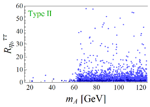
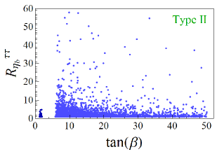
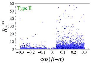
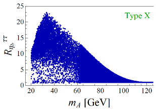
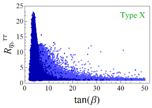
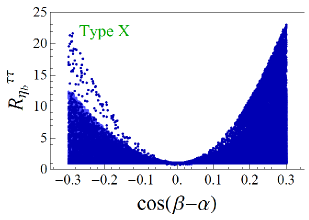
Figure 5: Results of the scan of parameters (34) after imposing constraints discussed in the text. Darker/lighter points correspond to the free/fine-tuned scan.

Finally, it is worth mentioning a correlation between $R^{\tau\tau}_{\eta_{c}}$ and $R^{\tau\tau}_{\eta_{b}}$ in Type I and Type X models, which is shown in Fig. 6. It is easy to understand its origin once one realizes that $\Gamma(h\to PA^{\ast}\to P\ell^{+}\ell^{-})$ dominates the full decay rate (14), and since the couplings to charm and to bottom quarks are equal in both models, $|\xi^{c}_{A}|=|\xi^{b}_{A}|=1/\tan\beta$, the correlation becomes quite obvious. Similar reasoning, but this time with respect to $\xi^{\tau}_{A}$, can be used to explain why the enhancement in Type X model ($|\xi^{\tau}_{A}|=\tan\beta$) is much more pronounced than the one in Type I model ($|\xi^{\tau}_{A}|=1/\tan\beta$).

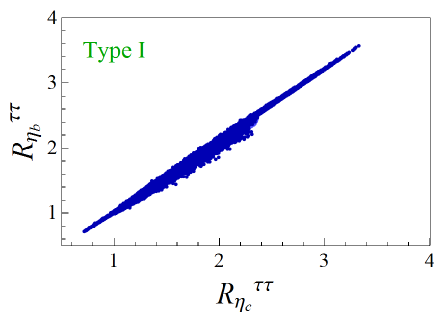
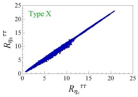
Figure 6: Correlation of the ratios $R^{\tau\tau}_{\eta_{c}}$ and $R^{\tau\tau}_{\eta_{b}}$ in Type I and Type X models arises from the fact that the Yukawa couplings of the charm and bottom quarks to the CP-odd Higgs are equal in these two models.

5 Summary and Conclusion

In this paper we elaborated on a possibility to search the signal of a light CP-odd Higgs state through the decays $h\to PZ$ and $h\to P\ell^{+}\ell^{-}$, with $P$ being either $\eta_{c}$ or $\eta_{b}$. We derived the relevant expressions, identified the dominant parts of the decay amplitudes and then focused on various types of the 2HDM. In our scan of the 2HDM parameter space we fixed $m_{h}=125.09(24)$ GeV and varied other parameters in the ranges indicated in Eq. (34), and then selected them as acceptable if consistent with a number of general theoretical constraints to which we also added those coming from the exclusive $b\to s\mu^{+}\mu^{-}$ modes [23] as well as the one arising from the inclusive $b\to s\gamma$ decay. That latter mode provides a substantial shift of the lower bound on $m_{H^{\pm}}$ in Type II and Type Z models [22].

We find that most of the branching fractions are either consistent with their Standard Model values or can get lowered (increased) by about $30\%$ ($10\%$). Notable exceptions are the models of Type I, II and X, in which the enhancement can be as large as a factor of $\sim 3$, and even a factor $\sim 20$, as highlighted in Tab. 2 where we summarized the numerical results of our study. The origin of that enhancement is due to $m_{A}\lesssim m_{h}$ and it is related to the Yukawa couplings to the CP-odd Higgs, which explains why the effect is so pronounced in the case of $\tau$-leptons in the final state (in contrast to the case of muons or electrons).

The large enhancement of ${\mathcal{B}}(h\to\eta_{b}\tau^{+}\tau^{-})$ in Type II and Type X models as high as a factor $\approx 20$ with respect to its Standard Model value is also possible in the case of ${\mathcal{B}}(h\to\eta_{c}\tau^{+}\tau^{-})$, but only in the Type X model, which is a consequence of the structure of Yukawa couplings and the amplitude mediated by $h\to AA$ vertex in the decay. While in this paper we focused on the decay of the SM Higgs boson, one could also consider a production of Higgs associated with the quarkonium state, along the lines similar to what has been discussed in Ref. [26].

We should also add that in this paper we focused on the lowest lying pseudoscalar quarkonia, but that our discussion could be trivially extended to the excited pseudoscalar quarkonia. Strategies for their detections have been discussed in Ref. [27] and references therein.

Appendix A Expressions for the amplitudes considered

We show here expressions for the direct contributions from diagrams in Figs. 1a, 2a and 3a, and the indirect contributions involving leptons in Figs. 1b, 2b.

The amplitude for the diagrams in Figs. 1a, 2a and 3a where the Higgs couples directly to the quark and anti-quark pair from which the meson is formed can be calculated in the QCD factorization approach, with the bound state effect of the highly energetic hadrons in the final state accounted for in terms of light-cone distribution amplitudes (LCDA) of these hadrons. The light-cone projector for a pseudoscalar meson $P$ in momentum space, defined in terms of the matrix elements of the non-local quark and gluon current, up to twist-3 can be written as [28, 29],

$$M_{P}(k,x,\mu) = \frac{if_{P}}{4}\left\{\not{k}\gamma_{5}\phi_{P}(x,\mu)-\mu_{P}(\mu)\gamma_{5}\left[\phi_{p}(x,\mu)-i\sigma_{\mu\nu}\frac{k^{\mu}\bar{n}^{\nu}}{k\cdot\bar{n}}\frac{\phi^{\prime}_{\sigma}(x,\mu)}{6}\right.\right.$$ (40)

$$\left.\left.+i\sigma_{\mu\nu}k^{\mu}\frac{\phi_{\sigma}(x,\mu)}{6}\frac{\partial}{\partial k_{\perp\nu}}\right]+3{\rm-particle\leavevmode\nobreak\ LCDAs}\right\},$$

where $x$ is the longitudinal momentum fraction of meson carried by one of the valence quarks $q$, $\mu_{P}(\mu)=m_{P}^{2}/(2m_{q}(\mu))$, $\phi_{P}$ is the twist-2 LCDA, $\phi_{p,\sigma}$ are the two-particle twist-3 LCDAs, while the three-particle ones are neglected which is often referred to as Wandzura-Wilczek approximation [30], which amounts to:

$$\phi_{p}(x,\mu)=1,\leavevmode\nobreak\ \leavevmode\nobreak\ \leavevmode\nobreak\ \leavevmode\nobreak\ \phi_{\sigma}(x,\mu)=6x(1-x).$$ (41)

The light-like vector $\bar{n}$ in the above expression is aligned into the opposite direction of $\vec{k}$.

We have used the following definition in the calculation of amplitudes for the diagrams in Figs. 1a, 2a and 3a which involve the integrals over the LCDA of the pseudoscalar meson:

$$I_{1}(x,y) =\frac{1}{\mathcal{P}(x,1-x,y)}+\frac{1}{\mathcal{P}(1-x,x,y)},\quad I_{3}(x,y)=\frac{1}{\mathcal{P}(x,1-x,y)^{2}}+\frac{1}{\mathcal{P}(1-x,x,y)^{2}},$$

$$I_{2}(x,y) =\frac{x}{\mathcal{P}(x,1-x,y)}+\frac{1-x}{\mathcal{P}(1-x,x,y)},\quad I_{4}(x,y)=\frac{x}{\mathcal{P}(x,1-x,y)^{2}}+\frac{1-x}{\mathcal{P}(1-x,x,y)^{2}},$$

$$\bar{I}_{2}(x,y) =\frac{1-x}{\mathcal{P}(x,1-x,y)}+\frac{x}{\mathcal{P}(1-x,x,y)},\quad\bar{I}_{4}(x,y)=\frac{1-x}{\mathcal{P}(x,1-x,y)^{2}}+\frac{x}{\mathcal{P}(1-x,x,y)^{2}},$$ (42)

where $\mathcal{P}(a,b,y)=(a\leavevmode\nobreak\ m_{h}^{2}+b\leavevmode\nobreak\ y^{2}-a\leavevmode\nobreak\ b\leavevmode\nobreak\ m_{P}^{2}-m_{q}^{2})/m_{h}^{2}$. The expressions below are listed for the asymptotic form of the leading-twist LCDA, $\phi_{P}(x,\mu)=6x(1-x)$.

The direct contribution to the $h\rightarrow PZ$ decay amplitude, including the light cone projector at leading and sub-leading twist is,

$$F^{PZ}_{D} =-f_{P}\leavevmode\nobreak\ \frac{m_{q}}{2m_{h}^{2}}g_{A}^{q}\int_{0}^{1}dx\left[m_{q}\phi_{P}(x,\mu)I_{1}(x,m_{Z})-\mu_{P}(\mu)\left\{\phi_{p}(x,\mu)I_{2}(x,m_{Z})\right.\right.$$

$$\left.\left.+\frac{\phi_{\sigma}(x,\mu)}{6}\left(3I_{1}(x,m_{Z})-2r_{Z}I_{3}(x,m_{Z})-\frac{2}{m_{h}^{2}}(k\cdot p_{Z})I_{4}(x,m_{Z})\right)\right\}\right]$$

$$=f_{P}\leavevmode\nobreak\ g_{A}^{q}\leavevmode\nobreak\ \frac{m_{q}}{m_{h}^{2}}\left[2\mu_{P}(\mu)-3m_{q}\right]\frac{1-r_{Z}^{2}+2r_{Z}\leavevmode\nobreak\ {\rm ln}\leavevmode\nobreak\ r_{Z}}{(1-r_{Z})^{3}},$$ (43)

where $g_{A}^{q}$ is the axial-vector coupling of the $Z$ boson to the constituent quark of the meson, $k\cdot p_{Z}=m_{h}^{2}(1-r_{Z}-r_{P})/2$ and $r_{X}=m_{X}^{2}/m_{h}^{2}$, $X=Z,P,q$. This direct contribution is completely negligible as it is suppressed relative to the leading term in Eq. (2) by a factor of $m_{P}^{2}/m_{h}^{2}$ or $m_{q}^{2}/m_{h}^{2}$. We have also checked that the effect of the CP-violating coupling of the quarks to $h$ if present cannot be seen in these two body decays.

We next list the direct contribution to the three body Higgs decays Figs. 2a and 3a, along with the indirect contribution where the Higgs couples to the leptons Figs. 2b and 3b.

$$\mathcal{M}(h\to P\ell^{+}\ell^{-})^{2a} =f_{P}\frac{m_{q}}{vm_{h}^{2}}\left(\frac{g}{2\cos\theta_{W}}\right)^{2}\frac{g_{A}^{q}}{(q^{2}-m_{Z}^{2}+im_{Z}\Gamma_{Z})}$$

$$\left[\left(\mathcal{C}_{1}\leavevmode\nobreak\ k^{\mu}+\mathcal{C}_{2}\leavevmode\nobreak\ p^{\mu}\right)\left(-g_{\mu\nu}+\frac{q_{\mu}q_{\nu}}{m_{Z}^{2}}\right)\left(\bar{u}_{\ell}\gamma^{\nu}(g_{V}^{\ell}-g_{A}^{\ell}\gamma_{5})v_{\ell}\right)\right],$$ (44)

$$\mathcal{M}(h\to P\ell^{+}\ell^{-})^{2b} =f_{P}\frac{m_{\ell}}{v}\left(\frac{g}{2\cos\theta_{W}}\right)^{2}\frac{g^{q}_{A}}{(k^{2}-m_{Z}^{2}+im_{Z}\Gamma_{Z})}\left[k^{\mu}\left(-g_{\mu\nu}+\frac{k_{\mu}k_{\nu}}{m_{Z}^{2}}\right)\right.$$

$$\left.\left\{\frac{1}{(k+p_{\ell})^{2}}\left(\bar{u}_{\ell}\gamma^{\nu}(g_{V}^{\ell}-g_{A}^{\ell}\gamma_{5})(\not{k}+\not{p}_{\ell})v_{\ell}\right)\right.\right.$$

$$+\left.\left.\frac{1}{(k+p_{\bar{\ell}})^{2}}\left(\bar{u}_{\ell}(\not{k}+\not{p}_{\bar{\ell}})\gamma^{\nu}(g_{V}^{\ell}-g_{A}^{\ell}\gamma_{5})v_{\ell}\right)\right\}\right],$$ (45)

$$\mathcal{M}(h\to P\ell^{+}\ell^{-})^{3a} =-f_{P}\frac{m_{\ell}m_{q}^{2}}{v^{3}m_{h}^{2}}\frac{\xi^{\ell}_{A}\xi^{q}_{A}}{(q^{2}-m_{A}^{2}+im_{A}\Gamma_{A})}\mathcal{F}^{P\ell^{+}\ell^{-}}_{A}\left(\bar{u}_{\ell}\gamma_{5}v_{\ell}\right),$$ (46)

$$\mathcal{M}(h\to P\ell^{+}\ell^{-})^{3b} =f_{P}\mu_{P}(\mu)\frac{m_{\ell}^{2}m_{q}}{v^{3}}\frac{\xi^{\ell}_{A}\xi^{q}_{A}}{(k^{2}-m_{A}^{2}+im_{A}\Gamma_{A})}$$

$$\left\{\frac{1}{(k+p_{\ell})^{2}}\left[\bar{u}_{\ell}\gamma_{5}(\not{k}+\not{p}_{\ell})v_{\ell}\right]+\frac{1}{(k+p_{\bar{\ell}})^{2}}\left[\bar{u}_{\ell}(\not{k}+\not{p}_{\bar{\ell}})\gamma_{5}v_{\ell}\right]\right\},$$ (47)

where we have

$$\mathcal{C}_{1} =f_{P}\leavevmode\nobreak\ \frac{m_{q}}{2m_{h}^{2}}g_{A}^{q}\int_{0}^{1}dx\left[m_{q}\phi_{P}(x,\mu)I_{1}(x,q)-\mu_{P}(\mu)\left\{-\phi_{p}(x,\mu)\bar{I}_{2}(x,q)\right.\right.$$

$$\left.\left.+\frac{\phi_{\sigma}(x,\mu)}{6}\left(3I_{1}(x,q)-2I_{3}(x,q)+2\frac{(k\cdot p)}{m_{h}^{2}}\bar{I}_{4}(x,q)\right)\right\}\right]$$ (48)

$$=\frac{1}{m_{h}(1-r_{q})^{4}}\left\{(r_{q}-1)\left[6m_{q}m_{h}(r_{q}^{2}-1)-\mu_{P}(\mu)\left(2E_{P}(r_{q}+5)+m_{h}(r_{q}-1)(r_{q}+13)\right)\right]\right.$$

$$\left.+2\leavevmode\nobreak\ {\rm ln}\leavevmode\nobreak\ r_{q}\left[2E_{P}\mu_{P}(\mu)(2r_{q}+1)+m_{h}(r_{q}-1)(\mu_{P}(\mu)(4r_{q}+3)-6m_{q}r_{q})\right]\right\},$$

$$\mathcal{C}_{2} =f_{P}\leavevmode\nobreak\ \frac{m_{q}}{2m_{h}^{2}}g_{A}^{q}\int_{0}^{1}dx\left[-\mu_{P}(\mu)\left\{\phi_{p}(x,\mu)I_{1}(x,q)\right.\right.$$

$$\left.\left.\quad\qquad\qquad+\frac{\phi_{\sigma}(x,\mu)}{6}\left(2\frac{(p_{P}\cdot p_{h})}{m_{h}^{2}}I_{3}(x,q)-2r_{P}\bar{I}_{4}(x,q)\right)\right\}\right]$$

$$=\frac{2\mu_{P}(\mu)}{m_{h}(1-r_{q})^{3}}\left[2E_{P}(1+r_{q})+m_{h}(1-r_{q})^{2}+4E_{P}(1-r_{q})\right]\,,$$

$$\mathcal{F}^{P\ell^{+}\ell^{-}}_{A} =\int_{0}^{1}dx\left\{\phi_{P}(x,\mu)\left[m_{h}^{2}r_{P}I_{2}(x,q)+(k\cdot q)I_{1}(x,q)\right]-\mu_{P}(\mu)\phi_{p}(x,\mu)m_{q}I_{1}(x,q)\right\}$$

$$=-\frac{2}{(1-r_{q})^{3}}\left[3\left((1-r_{q}^{2})+2r_{q}{\rm ln}\leavevmode\nobreak\ r_{q}\right)(k\cdot q)+\mu_{P}(\mu)m_{q}(1-r_{q}^{2}){\rm ln}\leavevmode\nobreak\ r_{q}\right],$$ (49)

and $k\cdot q=1/2(m_{h}^{2}-m_{P}^{2}-q^{2})$, $k\cdot p=m_{h}E_{P}$, with $E_{P}=1/(2m_{h})(m_{h}^{2}+m_{P}^{2}-q^{2})$. The amplitudes for Fig. 2a [2b] listed in Eqs. (44) [(45)] being proportional to $m_{q}$ ($m_{\ell}$) can be safely neglected compared to Fig. 2(c), which is proportional to $m_{Z}$, Eq. (2.2). The CP-violating coupling of the fermions to $h$ if present will contribute to $P\ell^{+}\ell^{-}$ final state, through the trilinear Higgs ($hhh$) coupling. We find that the $h\rightarrow P\ell^{+}\ell^{-}$ is insensitive to the CP-odd coupling, the reason being it enters quadratically and is proportional to the mass of the final state fermions.

References

- [1] G. C. Branco, P. M. Ferreira, L. Lavoura, M. N. Rebelo, M. Sher and J. P. Silva, Phys. Rept. 516, 1 (2012) [arXiv:1106.0034 [hep-ph]]; I. P. Ivanov, arXiv:1702.03776 [hep-ph].
- [2] G. Aad et al. [ATLAS and CMS Collaborations], Phys. Rev. Lett. 114 (2015) 191803 [arXiv:1503.07589 [hep-ex]].
- [3] R. Enberg, W. Klemm, S. Moretti and S. Munir, Phys. Lett. B 764 (2017) 121 [arXiv:1605.02498 [hep-ph]]; J. Bernon, J. F. Gunion, H. E. Haber, Y. Jiang and S. Kraml, Phys. Rev. D 93 (2016) no.3, 035027 [arXiv:1511.03682 [hep-ph]].
- [4] A. G. Akeroyd et al., arXiv:1607.01320 [hep-ph].
- [5] R. Dermisek and J. F. Gunion, Phys. Rev. D 81 (2010) 055001 [arXiv:0911.2460 [hep-ph]]. ibid 81 (2010) 075003 [arXiv:1002.1971 [hep-ph]]; S. Chang, R. Dermisek, J. F. Gunion and N. Weiner, Ann. Rev. Nucl. Part. Sci. 58 (2008) 75 [arXiv:0801.4554 [hep-ph]]; R. Dermisek, E. Lunghi and A. Raval, JHEP 1304 (2013) 063 [arXiv:1212.5021 [hep-ph]].
- [6] U. Ellwanger, Eur. Phys. J. C 71 (2011) 1782 [arXiv:1108.0157 [hep-ph]]; D. Curtin et al., Phys. Rev. D 90 (2014) no.7, 075004 [arXiv:1312.4992 [hep-ph]].
- [7] F. Domingo, U. Ellwanger, E. Fullana, C. Hugonie and M. A. Sanchis-Lozano, JHEP 0901 (2009) 061 [arXiv:0810.4736 [hep-ph]]; F. Domingo, JHEP 1703 (2017) 052 [arXiv:1612.06538 [hep-ph]].
- [8] U. Haisch and J. F. Kamenik, Phys. Rev. D 93 (2016) no.5, 055047 [arXiv:1601.05110 [hep-ph]].
- [9] G. T. Bodwin, F. Petriello, S. Stoynev and M. Velasco, Phys. Rev. D 88, no. 5, 053003 (2013) [arXiv:1306.5770 [hep-ph]]; M. Konig and M. Neubert, JHEP 1508, 012 (2015) [arXiv:1505.03870 [hep-ph]].
- [10] D. N. Gao, Phys. Lett. B 737, 366 (2014) [arXiv:1406.7102 [hep-ph]].
- [11] S. Alte, M. Konig and M. Neubert, JHEP 1612, 037 (2016) [arXiv:1609.06310 [hep-ph]].
- [12] P. Colangelo, F. De Fazio and P. Santorelli, Phys. Lett. B 760, 335 (2016) [arXiv:1602.01372 [hep-ph]].
- [13] C. Patrignani et al. [Particle Data Group], Chin. Phys. C 40 (2016) no.10, 100001.
- [14] S. L. Glashow and S. Weinberg, Phys. Rev. D 15 (1977) 1958.
- [15] J. F. Gunion and H. E. Haber, Phys. Rev. D 67, 075019 (2003) [hep-ph/0207010].
- [16] A. Barroso, P. M. Ferreira, I. P. Ivanov and R. Santos, JHEP 1306, 045 (2013) [arXiv:1303.5098 [hep-ph]].
- [17] S. Kanemura, T. Kubota and E. Takasugi, Phys. Lett. B 313, 155 (1993) [hep-ph/9303263].
- [18] B. Świeżewska, Phys. Rev. D 88, no. 5, 055027 (2013) Erratum: [Phys. Rev. D 88, no. 11, 119903 (2013)] [arXiv:1209.5725 [hep-ph]].
- [19] R. Barbieri, L. J. Hall, Y. Nomura and V. S. Rychkov, Phys. Rev. D 75, 035007 (2007) [hep-ph/0607332].
- [20] M. Baak et al. [Gfitter Group], Eur. Phys. J. C 74, 3046 (2014) [arXiv:1407.3792 [hep-ph]].
- [21] T. Corbett, O. J. P. Eboli, D. Goncalves, J. Gonzalez-Fraile, T. Plehn and M. Rauch, JHEP 1508, 156 (2015) [arXiv:1505.05516 [hep-ph]].
- [22] M. Misiak and M. Steinhauser, Eur. Phys. J. C 77 (2017) no.3, 201 [arXiv:1702.04571 [hep-ph]].
- [23] P. Arnan, D. Bečirević, F. Mescia and O. Sumensari, arXiv:1703.03426 [hep-ph].
- [24] D. Bečirević, G. Duplančić, B. Klajn, B. Melić and F. Sanfilippo, Nucl. Phys. B 883 (2014) 306 [arXiv:1312.2858 [hep-ph]].
- [25] C. McNeile, C. T. H. Davies, E. Follana, K. Hornbostel and G. P. Lepage, Phys. Rev. D 86 (2012) 074503 [arXiv:1207.0994 [hep-lat]].
- [26] I. Brivio, F. Goertz and G. Isidori, Phys. Rev. Lett. 115 (2015) no.21, 211801 [arXiv:1507.02916 [hep-ph]].
- [27] S. Godfrey and K. Moats, Phys. Rev. D 92 (2015) no.5, 054034 [arXiv:1507.00024 [hep-ph]].
- [28] M. Beneke, G. Buchalla, M. Neubert and C. T. Sachrajda, Nucl. Phys. B 606, 245 (2001) [hep-ph/0104110].
- [29] Y. Grossman, M. Konig and M. Neubert, JHEP 1504, 101 (2015) [arXiv:1501.06569 [hep-ph]].
- [30] S. Wandzura and F. Wilczek, Phys. Lett. 72B, 195 (1977).