Amplitude-dependent topological edge states in nonlinear phononic lattices

Abstract

This work investigates the effect of nonlinearities on topologically protected edge states in one and two-dimensional phononic lattices. We first show that localized modes arise at the interface between two spring-mass chains that are inverted copies of each other. Explicit expressions derived for the frequencies of the localized modes guide the study of the effect of cubic nonlinearities on the resonant characteristics of the interface which are shown to be described by a Duffing-like equation. Nonlinearities produce amplitude-dependent frequency shifts, which in the case of a softening nonlinearity cause the localized mode to migrate to the bulk spectrum. The case of a hexagonal lattice implementing a phononic analogue of a crystal exhibiting the quantum spin Hall effect is also investigated in the presence of weakly nonlinear cubic springs. An asymptotic analysis provides estimates of the amplitude dependence of the localized modes, while numerical simulations illustrate how the lattice response transitions from bulk-to-edge mode-dominated by varying the excitation amplitude. In contrast with the interface mode of the first example studies, this occurs both for hardening and softening springs. The results of this study provide a theoretical framework for the investigation of nonlinear effects that induce and control topologically protected wave-modes through nonlinear interactions and amplitude tuning.

I Introduction

Wave propagation in periodic media is an active field of research with applications in diverse areas of science and engineering. Phononic crystals allow superior wave manipulation and control compared to conventional bulk media, since they present directional bandgaps and highly anisotropic dynamic behavior. Potential applications include vibration control, surface acoustic wave devices and wave steering hussein2014dynamics . Recently, the achievement of defect-immune and scattering-free wave propagation using periodic media has received significant attention. The advent of topological mechanics huber2016topological provides an effective framework for the pursuit of robust wave propagation which is protected against perturbations and defects. Topologically protected edge wave propagation was originally envisioned in quantum systems and it has been quickly extended to other classical areas of physics, including acoustic brendel2017snowflake , photonic khanikaev2013photonic , optomechanical peano2014topological and elastic mousavi2015topologically ; pal2017edge media. The unique properties achieved in these media, such as immunity to backscattering and localization in the presence of defects and imperfections, are a result of band topology. These properties allow for lossless propagation of information, or waves confined to a boundary or interface. Therefore, they may be part of a fundamentally new mechanism for wave-based transport of information or energy.

There are two broad ways to realize topologically protected wave propagation in elastic media. The first one uses active components, thereby mimicking the quantum Hall effect. Changing of the parity of active devices or modulating of the physical properties in time have shown to alter the direction and nature of edge waves swinteck2015bulk ; nassar2017modulated . Examples include magnetic fields in biological systems prodan2009topological , rotating disks nash2015topological and acoustic circulators operating on the basis of a flow-induced bias khanikaev2015topologically . The second way uses solely passive components and relies on establishing analogues of the quantum spin Hall effect. These media feature both forward and backward propagating edge modes, which can be induced by an external excitation of appropriate polarization. The concept is illustrated in several studies by way of both numerical mousavi2015topologically ; pal2017edge ; pal2016helical ; he2016topological and experimental susstrunk2015observation ; ningyuan2015time investigations, which involve coupled pendulums susstrunk2015observation , plates with two scale holes mousavi2015topologically and resonators pal2017edge , as well as electric circuits ningyuan2015time . Numerous studies have also been conducted on localized non-propagating deformation modes at the interface of two structural lattices prodan2017dynamical ; pal2017edge ; chaunsali2017demonstrating . These modes depend on the topological properties of the bands, and in $1D$ lattices, they are characterized by the Zak phase as the topological invariant xiao2015geometric . In $2D$ and $3D$ lattices, several researchers have investigated the presence of floppy modes of motion due to nontrivial topological polarization and exploited these modes to achieve localized buckling and directional response kane2014topological ; paulose2015selective ; rocklin2016mechanical ; rocklin2016directional .

While most studies consider systems governed by linear interactions, there is growing interest in the investigation of the effect of nonlinearities in topological materials. Nonlinearities, for example, enable tunable wave motion, which in turn may lead to non-reciprocal wave propagation fleury2014sound ; vila2017bloch . This finds potential applications in acoustic switching pal2014wave , diodes boechler2011bifurcation and delay lines alu2016metamaterials . Nonlinear effects have been investigated to demonstrate self-induced topological phase transitions in SSH (Su-Schrieffer-Heeger) hadad2016self . In the field of photonics, several studies have considered topological effects in nonlinear media. Included in these studies are soliton-like topological states which exist on the edges of weakly nonlinear photonic systems ablowitz2014linear ; leykam2016edge , or in the bulk and propagate around the edge of a self-induced defect lumer2013self . These solitons arise in systems that can be described by a nonlinear Schrodinger (NLS) equation ablowitz2014linear ; ablowitz2017tight ; lumer2013self ; leykam2016edge and coupled nonlinear SSH equations zhou2017optical , all obtained from a Kerr-like optical nonlinearity.

This work investigates the effect of nonlinearities on two types of topologically protected localized modes in phononic lattices. Specifically, we study the robustness and frequency content of localized modes in a $1D$ and $2D$ lattices. In the $1D$ lattice, we illustrate the amplitude-dependent resonant behavior of an interface mode, which can lead to its shifting into the bulk bands. In the $2D$ case, the perturbation approach of  narisetti2010perturbation ; Narisetti2011 is applied to predict the amplitude-dependent frequency of edge modes for both hardening and softening springs. In both cases, the predictions are verified through numerical simulations on finite lattices excited by forces of increasing amplitude.

The outline of this paper is as follows: Sec. II presents a discrete $1D$ lattice (chain) with an interface and explicit expressions for the frequency and mode shapes of modes localized at the interface. The corresponding tunable nonlinear chain version is discussed in Sec. II.2. Then we show how the lattice response can switch from bulk to edge waves at a fixed frequency by varying amplitude in a $2D$ lattice in Sec. III. The $2D$ designs are verified by a combination of dispersion analysis and numerical simulations on finite lattices. Finally, Sec. IV presents the conclusions of this study.

II Interface modes in a $1D$ lattice

We begin our investigations by illustrating the existence and behavior of interface modes in a $1D$ spring-mass chain. The linear case is presented first, in order to briefly describe the existence of localized modes at the interface of chains that are characterized by distinct topological invariants, which in this case is the Zak phase xiao2015geometric ; xiao2014surface . The analytical derivation of the interface mode frequencies are presented in Appendix A and details of the topological properties of the linear chain are provided in Appendix B. Next, the behavior of an interface with nonlinear interactions is investigated in detail through its representation as a simple, single degree of freedom oscillator. This approach enables the study of the effect of nonlinearities in relation to the existence of the interface mode as a function of the excitation amplitude, and specifically to its tendency to enter the bulk spectrum based on the parameters defining the nonlinear interactions.

II.1 Linear chain: Analytical and numerical results

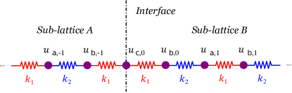
Figure 1: Two sub-lattices (A,B) which are inverted copies of each other, are joined together. The interface supports support a localized mode in the bandgap frequencies.

The spring mass chain model considered is displayed in Fig. 1. It consists of two sub-lattices, each with identical masses and having alternating springs with stiffness $k_{1}$ and $k_{2}$ and of an interface (or defect) mass connecting them. The interface mass is connected to springs with stiffness $k_{1}$ on both sides. The unit cells on the right and left of this interface are inverted copies of each other. This discrete lattice was investigated in pal2017edge , where the existence of two types of localized modes were discussed.

The governing equation for the free vibration of interface mass is

$$m\ddot{u}_{c,0}+k_{1}\left(2u_{c,0}-u_{b,0}-u_{b,1}\right)=0\\$$ (1)

Similarly, the governing equations for a unit cell $p$ of the sub-lattice on the left of the interface

$$m\ddot{u}_{a,p}+k_{2}\left(u_{a,p}-u_{b,p}\right)+k_{1}\left(u_{a,p}-u_{b,p-1}\right)=0$$ (2a)

$$m\ddot{u}_{b,p}+k_{2}\left(u_{b,p}-u_{a,p}\right)+k_{1}\left(u_{b,p}-u_{a,p+1}\right)=0$$ (2b)

while for a unit cell $p$ on the right sub-lattice are

$$m\ddot{u}_{a,p}+k_{1}\left(u_{a,p}-u_{b,p}\right)+k_{2}\left(u_{a,p}-u_{b,p-1}\right)=0$$ (3a)

$$m\ddot{u}_{b,p}+k_{1}\left(u_{b,p}-u_{a,p}\right)+k_{2}\left(u_{b,p}-u_{a,p+1}\right)=0.$$ (3b)

The above equations are normalized by writing the spring constants as $k_{1}=k(1+\gamma)$ and $k_{2}=k(1-\gamma)$, with $\gamma$ being a stiffness parameter and $k$ being the mean stiffness. A nondimensional time scale $\tau=\sqrt{k/m}t$ is introduced to express the equations in nondimensional form.

In the present work, explicit expressions for the frequency of the localized modes at the interface are derived by using a transfer matrix approach. The derivations can be found in Appendix A. These expressions allow us to identify and investigate the parameters affecting the frequency and modeshapes in a systematic way. They also shed light on the amplitude dependence (for $\gamma<0$) and independence (for $\gamma>0$) of the localized modes in chains with weakly nonlinear springs. Our theoretical predictions are verified through a combination of frequency domain analysis and transient numerical simulations on a finite chain with an interface.

The following are the solutions for the frequencies which support localized solutions

$$\begin{split}&\gamma<0:\quad\Omega=\sqrt{3-\sqrt{1+8\gamma^{2}}},\quad\textrm{Anti-symmetric mode}\\ &\gamma>0:\quad\Omega=\sqrt{2},\;\;\qquad\qquad\quad\quad\textrm{Symmetric mode}\\ &\gamma>0:\quad\Omega=\sqrt{3+\sqrt{1+8\gamma^{2}}},\quad\textrm{Anti-symmetric mode. }\end{split}$$ (4)

Here $\Omega$ is the non-dimensional frequency obtained by normalizing with the reference frequency $\sqrt{k/m}$. The detailed derivations of these frequencies along with their associated modeshapes are presented in appendix A. Note that the first and second solutions give frequencies which are localized in the bandgap between the acoustic and optical branches, while the third frequency is above the optical branch. Furthermore, the first and third frequencies are associated with anti-symmetric mode shapes where the unit cells on both sides of the interface are in phase, while the second frequency is associated with a symmetric mode shape, with the interface mass being at rest, while the unit cells on both sides have a phase difference of $\pi$.

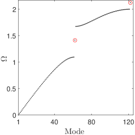
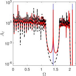
Figure 2: (a) Natural frequencies of a finite chain exhibiting interface modes (red circles) in the bandgap frequencies. (b) Frequency response function (red,solid) showing the interface mode within the bandgap, in agreement with analytical predictions (blue, dotted). Interface modes are absent in a regular chain with all identical unit cells (black, dashed).

We verify our analytical predictions by numerically computing the modes of oscillation of a finite chain having $60$ unit cells with an interface at the center, see Figure 1. The stiffness parameter is set to $\gamma=0.4$. The governing equations for our lattice may be written in matrix form as $\bm{M}\ddot{\bm{q}}(\tau)+\bm{K}\bm{q}(\tau)=\bm{f}(\tau)$. We seek the forced vibration response of the linear chain when subjected to an external force $\bm{f}\cos\Omega\tau$. Imposing a solution ansatz of the form $\bm{q}(\tau)=\bm{q}e^{i\Omega\tau}$, the governing equation reduces to

$$\left(\bm{K}-\Omega^{2}\bm{M}\right)\bm{q}=\bm{f}.$$ (5)

Figure 2 displays the natural frequencies $\Omega$ of this chain, obtained by solving the eigenvalue problem that arises by setting $\bm{f}=0$. It illustrates the presence of a bandgap between the acoustic and optical modes. Furthermore, there is an interface mode in the bandgap at frequency $\Omega=\sqrt{2}$, which matches exactly with the analytical solution of $\Omega_{i}$ for $\gamma>0$ in Eqn. (23). Analogous results are obtained for the chain with $\gamma<0$, consistent with the analytical expressions for the localized mode frequencies and shapes.

To illustrate the dynamic behavior of this chain, we compute the frequency response function by imposing a displacement $u_{b,30}=\cos(\Omega\tau)$ on the mass at the left boundary. The other end of the chain is free and the frequency response is normalized with the excitation amplitude, which is unity in our study. We also consider a chain that has no interface and comprises $60$ identical unit cells (regular chain), in which edge modes are not expected. Figure 2 displays the displacement amplitude of the center mass for both chains obtained by solving Eqn. (5) with appropriate displacement boundary conditions $(\bm{f}=0)$ over a wide frequency range. In the bandgap frequency range, the regular chain with all identical unit cells does not support any resonance mode. The chain with an interface mass has a resonance mode, consistent with the analytical solution (Eqn. (23)).

II.1.1 Reduced model for forced response

We now seek the forced vibration response of a chain comprised of $N$ unit cells on each side of the interface. The interface mass is subjected to an external forcing $f$ at frequency $\Omega$. We consider the anti-symmetric mode that arises when $\gamma<0$, for which we derive a reduced order model when the interface mass is subjected to the external force. As shown in Eqn. (23), the interface mode is anti-symmetric, i.e., $u_{b,0}=u_{b,-1}$. Since the wavenumber is $\pi$ in the bandgaps and there is no propagation, this displacement relation is valid for frequencies in the bandgap when $\gamma<0$. The relation $\bm{u}_{N}=\bm{T}^{N}\bm{u}_{0}$ can be inverted to get the relation $\bm{u}_{0}=\bm{T}^{-N}\bm{u}_{N}$. We reduce the chain to a single degree of freedom system which governs the behavior of the interface mass and obtain an expression for the effective stiffness on the interface mass. Fixing the first and last masses of the chain ($u_{b,N}=u_{b,-N}=0$), the relation $\bm{u}_{0}=\bm{T}^{-N}\bm{u}_{N}$ simplifies to the equation $u_{b,0}/S_{12}=u_{c,0}/S_{11}$, where $S_{ij}$ are the components of $\bm{S}=\bm{T}^{-N}$. The governing equation of the interface mass is $(2(1+\gamma)-\Omega^{2})u_{c,0}-2(1+\gamma)u_{b,0}=f$. Eliminating $u_{b,0}$ from these two relations yields the following expression for the effective behavior of the interface mass

$$\left[2(1+\gamma)\left(1-\dfrac{S_{21}}{S_{11}}\right)-\Omega^{2}\right]u_{c,0}=f.$$ (6)

Explicit expressions for the terms $S_{11}$ and $S_{21}$ in terms of the excitation frequency $\Omega$ and $\gamma$ are presented in Appendix C.

The results for the interface frequency can be further generalized to the case of springs adjacent to the interface different from $k_{1}$ through a parameter $\chi$. The springs connected to the interface mass are changed to $\chi k_{1}$ while the stiffness of all the other springs in the chain remain unchanged. Figure 3 illustrates a schematic of this modified interface. The governing equation for the interface mass now becomes

$$-\Omega^{2}u_{c,0}+\chi(1+\gamma)(2u_{c,0}-u_{b,0}+u_{b,-1})=0.$$

Numerical analysis is performed to determine the natural frequencies of this modified interface using a chain of $60$ unit cells by solving the eigenvalue problem ($\bm{f}=\bm{0}$ in Eqn. (5)). The interface mode frequency is located by examining its corresponding mode shape. Figure 3 displays the interface mode frequency for three distinct $\chi$ values: $0.7$, $1$ and $2$ over a range of stiffness parameter values $\gamma$. Also shown by dashed lines are the frequencies bounding the bandgap. We observe that only the anti-symmetric mode ($\gamma<0$) frequency shifts, while the symmetric mode ($\gamma>0$) frequency remains unchanged. This surprising observation can be explained by examining the mode shape of the edge mode when $\gamma>0$. For this mode shape, the interface mass $(c,0)$ has zero displacement as the force acting on its either sides are equal and opposite. Thus changing the stiffness of the spring connecting $(c,0)$ from both sides does not affect the dynamic behavior of this mass. The displacement of the adjacent masses $u_{b,0}$ and $u_{b,-1}$ change in account of the increased stiffness. However the remaining mode shape and the corresponding frequency do not change with $\chi$.

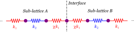
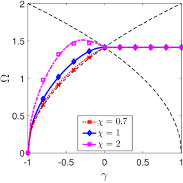
Figure 3: (a) Schematic of an interface having springs with modified stiffness $\chi k_{1}$. All other spring stiffnesses remain unchanged. (b) Variation of the interface frequency as a function of $\gamma$ for the $3$ distinct values of $\chi$ listed in the legend. Dashed curves show frequencies bounding the bandgap.

II.2 Analysis of nonlinear interface

Based on the above observations, we seek to achieve a tunable response in our chain by using nonlinear springs whose stiffness depends on the amplitude. An effect similar to the frequency shift due to springs with stiffness $\chi k_{1}$ in the above linear chain may be obtained by varying the excitation force amplitude. We consider a chain identical to the above linear chain with an interface, but replace the two interface springs having stiffness $\chi k_{1}$ with weakly nonlinear springs, whose restoring force varies with relative displacement $\Delta u$ as $F=k_{1}\Delta u+\Gamma(\Delta u)^{3}$. Adding a cubic nonlinearity leads to an amplitude-dependent frequency of the interface mode. Viscous damping with coefficient $c$ is applied to the mass at the interface so that a steady-state can be reached in our numerical simulations. We show how the nonlinear chain behaves essentially as a Duffing oscillator using a reduced order model for the interface mass, similar to Eqn. (6). Our analytical results thus provide the opportunity to apply known results on Duffing oscillators to the investigation of edge modes in nonlinear regimes.

We investigate the forced vibration response of this nonlinear chain subjected to an external excitation force $f$ applied at the interface mass. The governing equation for the mass at the interface and its adjacent masses may be written as

$$m\ddot{u}_{c,0}+c\dot{u}_{c,0}+k_{1}(2u_{c,0}-u_{b,0}-u_{b,-1})+$$

$$\qquad\Gamma\left(u_{c,0}-u_{b,0}\right)^{3}+\Gamma\left(u_{c,0}-u_{b,-1}\right)^{3}=f\cos(\Omega t),$$

$$m\ddot{u}_{b,0}+k_{1}\left(u_{b,0}-u_{c,0}\right)+k_{2}\left(u_{b,0}-u_{a,1}\right)+$$

$$\;\;\qquad\qquad\qquad\qquad\qquad\Gamma(u_{b,0}-u_{c,0})^{3}=0,$$ (7)

$$m\ddot{u}_{b,-1}+k_{1}\left(u_{b,-1}-u_{c,0}\right)+k_{2}\left(u_{b,-1}-u_{a,-1}\right)+$$

$$\qquad\qquad\qquad\qquad\qquad\Gamma(u_{b,-1}-u_{c,0})^{3}=0.$$

The governing equations for all the other masses on both sides of the interface remain the same as in the linear case (Eqns. (2), (3)). Again, we consider a chain with stiffness parameter $\gamma<0$ and derive the equivalent behavior of the interface mass in the bandgap frequencies.

To now get an equivalent equation for the interface mass, we need to eliminate $u_{b,0}$ from the governing equation of the interface mass. Let us assume an approximate solution for the displacement of the masses in the chain to be of the form

$$\bm{u}=\dfrac{\bm{v}e^{i\Omega t}}{2}+\epsilon\sum_{n=2}^{M}\left(\bm{w}_{n}e^{in\Omega\tau}\right)+c.c.,$$ (8)

with $\epsilon$ being a bookkeeping parameter and $c.c.$ denoting the complex conjugate. Recall that $e_{1}$ and $e_{2}$ are the components of the eigenvector corresponding to the localized mode in the linear chain (Eqn. (24)). The nonlinear force term may be approximated as

$$\Gamma(u_{c,0}-u_{b,0})^{3}=\dfrac{3}{8}\Gamma\left(1-\dfrac{e_{2}}{e_{1}}\right)^{3}|v_{c,0}|^{2}v_{c,0}e^{i\Omega t}+\epsilon(h.h.),$$ (9)

where $h.h.$ denotes higher harmonics. Note that the above approximation is valid for small displacements when the term $u_{b,0}/u_{c,0}$ can be approximated by the linear solution ($\bm{u}_{0}=s\bm{e}$).

We perform a harmonic balance on the linear parts of the chain by considering only the terms of frequency $\Omega$. The displacements in the linear parts of the chain can be related using the transfer matrix approach. Observe that the structure of the chain results in exactly the same relation as Eqn. (A) holding between $(v_{b,p-1},v_{a,p})$ and $(v_{b,p},v_{a,p+1})$ under the transformation $\gamma\to-\gamma$. Thus, defining the corresponding quantities $\overline{\bm{S}}(\gamma)=\bm{S}(-\gamma)=\bm{T}^{-N}(-\gamma)$ leads to the following relation

$$\overline{S}_{12}v_{b,0}-\overline{S}_{11}v_{a,1}=0.$$ (10)

Imposing Eqn. (8) and again performing a harmonic balance, the equation for the displacement $v_{b,0}$ of the mass adjacent to the interface mass now becomes

$$-\Omega^{2}v_{b,0}+(1+\gamma)\left(v_{b,0}-v_{c,0}\right)+(1-\gamma)\left(v_{b,0}-v_{a,1}\right)\\ -\dfrac{3\Gamma}{4}\left(1-\dfrac{e_{2}}{e_{1}}\right)^{3}|v_{c,0}|^{2}v_{c,0}=0,$$

Eliminating $v_{a,1}$ from the above equation using Eqn. (10), it may be rewritten as

$$\left[2-\Omega^{2}-(1-\gamma)\dfrac{\overline{S}_{12}}{\overline{S}_{11}}\right]v_{b,0}=\\ \dfrac{3\Gamma}{4}\left(1-\dfrac{e_{2}}{e_{1}}\right)^{3}|v_{c,0}|^{2}v_{c,0}+(1+\gamma)v_{c,0}.$$ (11)

We may write an equation similar to Eqn. (11) for the displacement $u_{b,-1}$ of the mass at the left of the interface mass and use an approximation similar to Eqn. (9) to simplify its cubic nonlinear term. Indeed, for the case $\gamma<0$, recall that the zeroth order solution is an anti-symmetric mode and thus $v_{b,0}=v_{b,-1}$. Substituting Eqn. (11) and its counterpart for $u_{b,-1}$ into the governing equation for the interface mass and performing a harmonic balance again leads to the following equation

$$-\Omega^{2}{v}_{c,0}+i\Omega\delta v_{c,0}+(1+\gamma)\left(2-\dfrac{1+\gamma}{g}\right)v_{c,0}+\\ \dfrac{3\Gamma}{4}\left(1-\dfrac{1+\gamma}{g}\right)\left(1-\dfrac{e_{2}}{e_{1}}\right)^{3}|v_{c,0}|^{2}v_{c,0}=f,$$ (12)

where $g=2-\Omega^{2}-(1-\gamma)\overline{S}_{12}/\overline{S}_{11}$ and $\delta=c\sqrt{2/km}$ is the nondimensional damping parameter. Decomposing $v_{0,c}=v_{R}+iv_{I}$ into its real and imaginary parts leads to two equations. Squaring and summing them leads to the following frequency amplitude response nayfeh2008perturbation

$$\left[\left(\Omega^{2}-k_{e}-\dfrac{3}{4}\Gamma_{e}u^{2}\right)^{2}+(\delta\Omega)^{2}\right]u^{2}=f^{2},$$ (13)

with $u=|v_{0,c}|$ being the displacement amplitude and

$$k_{e}=(1+\gamma)\left(2-\dfrac{1+\gamma}{g}\right),$$

$$\Gamma_{e}=\Gamma\left(1-\dfrac{1+\gamma}{g}\right)\left(1-\dfrac{e_{2}}{e_{1}}\right)^{3}.$$

The above frequency amplitude response is similar to that of a Duffing oscillator with linear stiffness $k_{e}$ and nonlinear force $\Gamma_{e}$ excited near the resonant frequency nayfeh2008perturbation .

Let us first consider a chain with strain hardening springs ($\Gamma>0$) connected to the interface mass. The dynamic response of the chain is investigated using the amplitude-response predicted by the reduced order model (Eqn. (13)) and transient simulations of the full nonlinear chain, performed using the Verlet algorithm Verlet67 . We compare the frequency response function predicted by the reduced order model with numerical simulations on a finite chain. The numerical simulations are performed until the chain attains a steady state. The damping coefficient, linear and nonlinear stiffness parameter values are set to $\delta=0.01$, $\gamma=0.4$ and $\Gamma=0.1$, respectively. The interface mass is subjected to an external force $f\cos(\Omega\tau)$. The frequency response is computed by normalizing the displacement $u_{c,0}$ of the interface mass by the excitation force amplitude $f$ as $A_{I}=u_{c,0}k/f$.

Figure 4 displays the frequency response of a finite linear chain (red curve) over $\Omega\in[0,\;2]$ along with the response observed from simulations of the finite nonlinear chain (black circles) for frequencies in the vicinity of the interface mode frequency, when subjected to low amplitude excitation ($f_{0}=1$). The linear chain response is obtained by solving the forced vibration response at steady state using Eqn. (5). Since the excitation force amplitude is low, nonlinear effects are seen to be negligible, and the predictions of the linear model are in good agreement with the numerical simulations for frequencies near the interface mode frequency.

Figure 4 displays a close up view of the frequency response computed from simulations of the finite nonlinear chain (markers), along with the response given by Eqn. (13), the nonlinear reduced order model (solid curves), for various force excitation amplitudes $f=\{1,4,10,25\}$. An excellent agreement is obtained between them which confirms the validity of our reduced order model. The peak force shifts to the right with increasing force amplitude and displays a backbone curve. This behavior is typical of a Duffing oscillator nayfeh2008perturbation and demonstrates the amplitude dependent behavior of the interface mode.

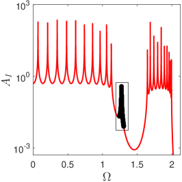
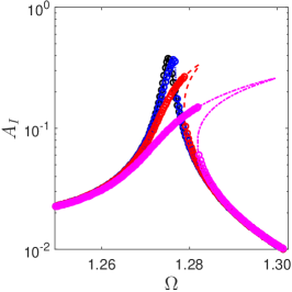
Figure 4: Frequency response of the interface mass normalized by excitation force $f$. (a) Both finite chain numerical simulations (red curve) and analytical solution of reduced model (black circles) show an interface mode for small forcing amplitude $f=1$. (b) Numerical (markers) and analytical (curves) solutions for various force amplitudes $f=\{1,4,10,25\}$. Curves shift to the right and the chain behaves as a Duffing oscillator for frequencies near the interface mode.

Let us now exploit the amplitude dependent behavior to migrate the localized mode into the bulk bands. By varying the amplitude, the localized mode can be eliminated from the bandgap frequencies. The damping coefficient, linear and nonlinear stiffness parameter values are set to $\delta=0.01$, $\gamma=-0.4$ and $\Gamma=-1$, respectively. Notice that strain softening springs ($\Gamma<0$) are used for this purpose. The interface mass in the chain is subjected to the same excitation as in the previous strain hardening case. Figure 5 displays the frequency response function for the displacement of the interface mass predicted by Eqn. (13) for three levels of forcing amplitude, (a) $f=0.006$, (b) $f=0.06$ and (c) $f=0.2$. The solid vertical lines depict the frequency bounds of the bandgaps, while the dashed (blue) vertical line shows the frequency of the interface mode when the chain is linear ($\Gamma=0$). The markers denote numerical solution obtained by solving the transient problem of an equivalent single degree of freedom Duffing oscillator until steady state (with stiffness parameters $k_{e}$ and $\Gamma_{e}$), while the solid curves denote the frequency amplitude response of Eqn. (13). The interface mode frequency and the normalized amplitude both decrease with increasing force amplitude, which is consistent with the behavior of a Duffing oscillator. As the amplitude increases, the frequency associated with the interface mode moves into the bulk bands from the bandgaps.

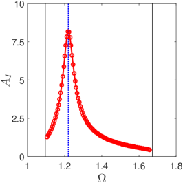
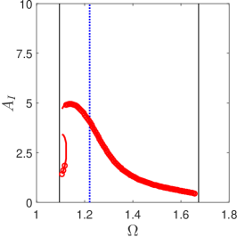
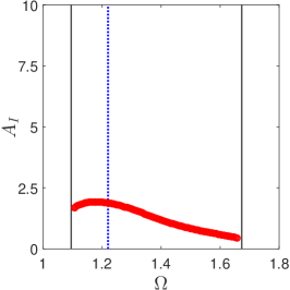
Figure 5: Analytical (curve) and numerical (circles) responses of a nonlinear chain exited at the interface with force amplitude $f$. The responses for various excitation amplitudes (a) $f=0.001$, (b) $f=0.06$ and (c) $f=0.2$, are normalized by $f$ and are distinct due to nonlinearity.

Having demonstrated how to shift the localized mode frequency into the bulk bands using a reduced single degree of freedom model, let us finally show how this shifting leads to a reduction in the response of a finite chain. We consider a chain of $20$ unit cells with an interface mass at the center and subject the mass at the left end to a harmonic displacement, while the mass at the right end is free. Figure 6 displays the normalized frequency response in the bandgap frequencies for two values of excitation force amplitude: $f=0.001$ (solid curves) and $f=0.06$ (dashed curves). Figure 6 displays a closeup of the frequency response near the interface mode frequency $\Omega_{i}$. The frequency response is similar to the linear case and nonlinear effects are negligible for small-amplitude excitations ($f\leq 0.001$), while moderate amplitudes ($f>0.01$) lead to a reduction in the displacement amplitude by an order of magnitude. The interface mode frequency shifts toward the lower end of the band-gap decreasing the response at the interface. Thus the frequency shifting behavior is demonstrated by first showing its analogy with a Duffing oscillator using our reduced model and then verifying these predictions with numerical simulations on a finite chain. In summary, amplitude dependent behavior and multiple stable solutions are observed for chains with stiffness parameter $\gamma<0$. This behavior is predicted analytically by showing the equivalence of the edge mode with a Duffing oscillator. Furthermore, edge mode frequency is independent of the wave amplitude for $\gamma>0$. This unexpected observation is explained by examining the analytical solution of eigenmodes associated with this edge mode.

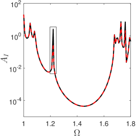
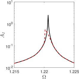
Figure 6: Transient response of a nonlinear chain with $\Gamma<0$ excited at one end. The normalized amplitude response in the bandgaps at high excitation amplitudes (dashed red line, $f=0.06$) is an order of magnitude lower than at low amplitudes (solid black line, $f=0.001$).

III Tunable edge modes in $2D$ lattices

We now extend the ideas presented in the previous section to $2D$ lattices. We consider the $2D$ lattice in Pal et. al. pal2016helical which implements a mechanical analogue of the quantum spin Hall effect and supports topologically protected edge modes. An amplitude dependent response is obtained by using weakly nonlinear springs. We present dispersion analysis of a unit cell and of an extended unit cell computed using an asymptotic analysis. In contrast to the interface mode in the $1D$ lattice, we show the ability of the considered lattice to undergo transitions from bulk-to-edge mode-dominated by varying the excitation amplitude both for hardening and softening springs. Finally, we present numerical simulations on finite lattices to illustrate the amplitude dependent nature of wave propagation due to nonlinearities.

III.1 Lattice configuration

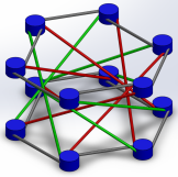
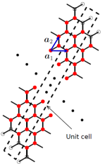
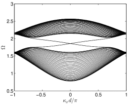
Figure 7: (a) A hexagonal cell of the lattice, having two layers with normal in-plane springs and a combination of normal and reverse springs between the two layers. (b) Finite strip with fixed boundaries. The nodes with filled (red) circles are free, while the others are fixed. (c) Dispersion diagram of the finite strip showing edge modes spanning the two sets of bulk modes.

The lattice consists of two layers of hexagonal lattice spanning the $xy$-plane. and its lattice vectors are $\bm{a}_{1}=(-1/2,\sqrt{3}/2)$ and $\bm{a}_{2}=(1/2,\sqrt{3}/2)$. Figure 7 displays a schematic of a single hexagonal cell. Each node is a disk that rotates about the $z$-axis, perpendicular to the plane of the lattice. Two kinds of springs, normal and chiral, connect the disks. The in-plane springs (gray color in Fig. 7) are linear and they provide a torque $k(\theta_{j}-\theta_{i})$ on disk $i$ due to rotations $\theta_{i}$ and $\theta_{j}$ of the two nearest neighbor disks connected to the spring. A combination of normal ($n$, green color in Fig. 7) and chiral ($ch$, red color in Fig. 7) springs connect the second nearest neighbors on adjacent layers in our lattice. These springs are weakly nonlinear and the torque-rotation relation between two disks $i,j$ are, respectively,

$$T^{n}_{i} =k_{n}(\theta_{j}-\theta_{i})+\epsilon_{n}(\theta_{j}-\theta_{i})^{3},$$ (14a)

$$T^{ch}_{i} =-k_{ch}(\theta_{j}+\theta_{i})-\epsilon_{ch}(\theta_{j}+\theta_{i})^{3}.$$ (14b)

III.2 Dispersion analysis of linear and nonlinear lattices

Dispersion studies are conducted both for a single hexagonal unit cell having $4$ degrees of freedom ($2$ in each layer) and for a unit cell of a strip which is periodic along one direction, as illustrated in Fig. 7. Let us set $\bm{u}$ as the vector whose components are the generalized displacement for all the degrees of freedom in a unit cell, which in our case, would be the rotation of disks at each lattice site. In pal2016helical , the authors show that this lattice has a band gap for bulk modes. Furthermore, there are topologically protected edge modes in this band gap which propagate along the boundaries of the lattice. We seek to investigate how weak nonlinearities affect the edge modes in our lattice. To get the dispersion relation of a nonlinear lattice, we use a perturbation based method to seek corrections to the linear dispersion relation $\omega=\omega(\bm{\mu})$, with $\bm{\mu}$ being the two dimensional wavevector. Based on the method of multiple scales, the following asymptotic expansion for the displacement components in a unit cell and frequency is imposed

$$\bm{u}=\bm{u}_{0}+\epsilon\bm{u}_{1}+O(\epsilon^{2}),$$

$$\omega=\omega_{0}+\epsilon\omega_{1}+O(\epsilon^{2}).$$

The asymptotic procedure we follow is similar to Leamy and coworkers narisetti2010perturbation ; Narisetti2011 and its details are presented in Appendix D.

We first present the dispersion behavior of a finite strip of a linear lattice to illustrate the existence of localized edge modes. Then, two kinds of nonlinear springs, strain hardening and strain softening, are considered to demonstrate the amplitude dependent nature of these edge modes. The equations are normalized using the time scale $\sqrt{k/I}$, with $I$ being the rotational inertia of the disks. In non-dimensional form (with superscript $\tilde{k}$), both the normal and chiral springs connecting adjacent layers are chosen to have a linear stiffness component $\tilde{k}_{n}=\tilde{k}_{ch}=0.1$ and their nonlinear components are equal ($\epsilon=\tilde{\epsilon}_{n}=\tilde{\epsilon}_{ch}$).

III.2.1 Dispersion analysis of a strip

To illustrate the presence of edge modes in our lattice, let us consider a finite strip of $20$ unit cells as illustrated in Fig. 7. The strip is periodic in the $\bm{a}_{1}$ direction and has a finite width in the $\bm{a}_{2}$ direction. The nodes with red (filled circle) markers are free to move, while the nodes with unfilled circles and squares at either boundary are fixed nodes. A dispersion analysis is conducted on this finite strip which is periodic in the $\bm{a}_{1}$ direction and the dashed rectangle shows the unit cell. By imposing a traveling wave solution of the form $\bm{u}=\bm{u}(\kappa_{x})e^{i(\Omega t-\kappa_{x}\cdot x)}$ on the lattice, an eigenvalue problem is obtained for each wavenumber $\kappa_{x}$. Note that the $x$-axis is oriented along the $\bm{a}_{1}$ direction.

Figure 7 displays the dispersion diagram for the finite strip under study. The wavenumber $\kappa_{1}$ is projected onto the $x$-axis. There are two sets of wave modes: the first set spans $[0.78,\;1.75]$ and the second set spans $[2.03,\;2.55]$. These two sets correspond to bulk modes and the two modes between them are edge modes. The eigenvectors corresponding to these frequencies are localized at the edges. We remark here on the choice of boundary conditions as shown in Fig. 7. Note that allowing the nodes with square markers to be free results in a different type of edge mode than the one illustrated in Fig. 7. The work in pal2016helical presented the band diagrams when the nodes having square markers were not fixed. There are two overlapping bands at each point in the dispersion diagrams in Fig. 7. The lattice supports two traveling waves at the edge of the lattice: one in the clockwise and the other in the counter-clockwise direction. Furthermore, these modes are topologically protected: they span the entire bandgaps and they cannot be localized by small disorders or perturbations hasan2010colloquium .

III.2.2 Strain hardening springs

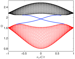
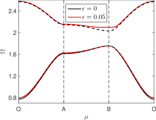
Figure 8: Dispersion diagram for both linear ($\epsilon=0$) and strain hardening springs $\epsilon=0.05$ over (a) a strip and (b) the irreducible Brillouin zone. The edge modes traverse the bandgaps and the optical band shifts upward near the point $B$ in the nonlinear lattice.

Having demonstrated the presence of edge modes in a linear lattice, we now investigate the effect of introducing nonlinear interactions between the interlayer springs. Figure 8 displays the dispersion diagram when the nonlinearity is of the strain hardening type $(\epsilon=0.05)$ with amplitude of the waves $A_{0}=0.6$. The first order correction is computed using an asymptotic analysis (Eqn. (36) in Appendix D) at each two dimensional wavevector $\bm{\mu}$ for both a unit cell in the bulk and a unit cell comprised of a finite strip. Figure 8 displays the bulk dispersion surface projected onto the $x$-axis along with the edge modes computed from the finite strip. A comparison with the dispersion diagram of the finite strip in the linear case shows that the lower band remains unchanged while the lower surface of the upper band shifts upward.

Figure 8 displays the dispersion curves along the boundary of the irreducible Brillouin zone for both the linear (dashed curves) and nonlinear (solid curves) lattices. Since the hexagonal lattice has a six-fold symmetry, the IBZ is a triangle and we choose it to span the points $O:(0,0)$, $A:(0,\pi)$ and $B:(2\pi/3,2\pi/3)$ in the reciprocal lattice space. The presence of inter-planar springs leads to a bandgap for bulk waves, as shown in Fig. 8 and the existence of edge waves in this bandgap. We see that the lower band does not get significantly affected due to the nonlinear springs. However, the upper band in the vicinity of point $B$ gets shifted upward and the bandgap widens as a consequence. Note that the edge modes continue to span the bandgaps and they do not localize (group velocity is nonzero) in the presence of nonlinear interactions.

We now elaborate how the above observations can be exploited to achieve amplitude dependent edge waves using our nonlinear lattices. At small amplitudes, the dynamic response is similar to a lattice with no nonlinear springs and corresponds to the $\epsilon=0$ case in Fig. 8. However as the amplitude increases, nonlinear effects come into play and the behavior resembles the nonlinear case, illustrated by $\epsilon=0.05$ in Fig. 8. Thus exciting at a frequency at the tip of the lower surface of the Brillouin zone near point $B$ will result in amplitude dependent edge waves. At small amplitudes, there will be no edge waves, while at high amplitudes, the band widens and one-way edge waves propagate in the lattice.

III.2.3 Strain softening springs

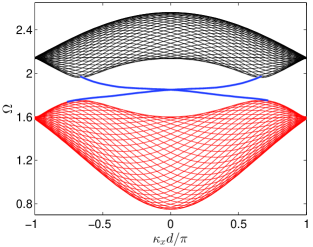
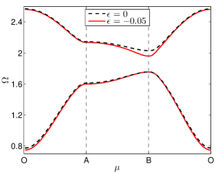
Figure 9: Dispersion diagram for lattices with linear ($\epsilon=0$) and strain softening springs $\epsilon=-0.05$ over (a) a strip and (b) the irreducible Brillouin zone. The edge modes traverse the bandgaps and the optical band shifts downward near the point $B$ in the nonlinear lattice.

We now turn attention to the study of nonlinear springs of the strain softening type having $\epsilon<0$. A similar dispersion analysis is conducted on both a strip and a single unit cell with nonlinear stiffness parameter $\epsilon=-0.5$ and wave amplitude $A_{0}=0.6$. Figure 9 displays the dispersion surface of both the bulk and edge modes projected onto the $x$-axis. Similar to the earlier case with $\epsilon>0$, the lower band does not change significantly due to the nonlinear springs. The lower surface of the upper band shifts downward, which is consistent with the behavior for $\epsilon>0$ case, since the first order correction $\epsilon\omega_{1}$ is linearly proportional to $\epsilon$. Figure 9 displays the dispersion curves along the boundary of the IBZ. In contrast with the strain hardening case, here the dispersion curves shift downward near the point $B$ while remaining relatively unaltered away from this point. Similar to the strain hardening case, these softening springs can be exploited to get amplitude dependent response of the lattice. The lattice behavior can be changed from edge waves at low amplitudes to bulk waves at high amplitudes. We thus illustrated the amplitude dependent nature of the dispersion curves for the strain softening nonlinear springs.

III.3 Numerical simulations of wave propagation

We now conduct numerical simulations to demonstrate the effect of nonlinear interactions on wave propagation in a finite lattice. The numerical results are interpreted using the dispersion diagrams for linear and nonlinear lattices that were presented earlier in Sec. III.2. All our numerical simulations are conducted on a lattice of $30\times 30$ unit cells using a fourth order Runge Kutta explicit time integration scheme. The boundary nodes of our lattice are fixed similar to that illustrated in Fig. 7. The lattice is subjected to a point excitation at a specific frequency on a boundary node lying at the center of the lower left boundary. Two examples are presented: the first one demonstrates edge wave propagation at high amplitudes, while the second example demonstrates the decaying of edge waves with increasing amplitude.

III.3.1 High amplitude edge waves

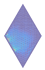
(a) $\;A=6\times 10^{-3},\;\tau=200$

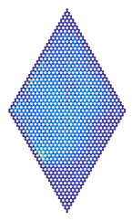
(b) $\;A=6\times 10^{-3},\;\tau=400$

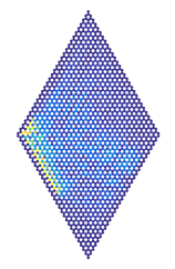
(c) $\;A=6\times 10^{-1},\;\tau=200$

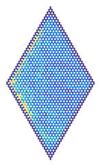
(d) $\;A=6\times 10^{-1},\;\tau=400$

Figure 10: Displacement magnitude at each lattice site at two time instants for lattice with $\epsilon=0.05$ subjected to two force amplitudes (a,b) $A=6\times 10^{-3}$, (c,d) $A=6\times 10^{-1}$ and excitation frequency $\Omega=2.045$. The lattice supports bulk and edge waves at low and high amplitudes, respectively.

In this example, the lattice comprises of nonlinear springs of the strain hardening type with $\epsilon=0.05$. Two numerical simulations are conducted: one at low ($A=6\times 10^{-3}$) and the other at high ($A=6\times 10^{-1}$) force excitation amplitudes. A boundary lattice site is subjected to to a harmonic excitation at frequency $\Omega=2.045$. The dispersion analysis in Fig. 8 shows that this frequency lies in the lower part of the top band and the linear lattice supports bulk waves and no edge waves. As discussed earlier in Sec. III.2.2, at higher amplitudes, the bandgap widens and edge modes exist at higher frequencies. The top and bottom layers are subject to the excitation

$$F_{top}=A\cos\omega t,\;\;F_{bottom}=A\sin\omega t.$$ (15)

Figure 10 displays the angular displacement of the disks at the various nodes. The color scale ranges for the two cases are $[0,8\times 10^{-3}]$ and $[0,8\times 10^{-1}]$. The colors show the magnitude ($l_{2}$ norm) of the displacement vector at each lattice site. Note that there are two disks (one at top and one at bottom layer) at each lattice site and the displacement vector thus has two components denoting the angular displacement of these two disks. Figures 10(a)-(b) display the displacement magnitude for the low amplitude excitation at times $\tau=200$ and $\tau=400$. It is observed that the wave propagation is isotropic from the point of excitation into the lattice and this behavior is consistent with the predictions of the dispersion analysis as there are no edge waves at the excitation frequency. Figures 10(c)-(d) displays the displacement magnitude for high amplitude excitation at the same time instants. Edge waves are observed to propagate in the counter-clockwise direction, which is indeed consistent with the behavior predicted in the dispersion analysis in Sec. III.2.2.

III.3.2 Bulk waves at high amplitudes

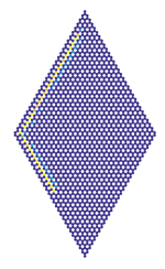
(a) $\;A=2\times 10^{-3},\tau=400$

(b) $A=2\times 10^{-3},\tau=1000$

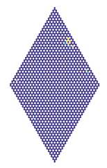
(c) $\;A=2\times 10^{-1},\tau=400$

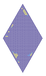
(d) $A=2\times 10^{-1},\tau=1000$

Figure 11: Displacement magnitude at each lattice site at two time instants for lattice with $\epsilon=0.05$ subjected to two force amplitudes (a,b) $A=2\times 10^{-3}$, (c,d) $A=2\times 10^{-1}$ and excitation frequency $\Omega=2.02$. The lattice supports edge waves at low amplitudes and bulk waves at high amplitudes. The color scale has a range (a,b): $[2.4\times 10^{-3},\;3\times 10^{-3}]$ and (c,d): $[2.4\times 10^{-1},\;3\times 10^{-1}]$.

Our next example involves strain softening springs having $\epsilon<0$. Again, the lattice is subjected to a point excitation at a frequency $\Omega=2.02$ with the top and bottom disks at the node having a phase difference of $\pi/2$ as in Eqn. (15). At this frequency, there are no bulk modes in the linear lattice and edge waves traverse through the lattice. As discussed in Sec. III.2.3, nonlinear interactions lead to shortening of the bandgap and edge modes do not propagate at high amplitudes.

Figures 11(a)-(b) display the displacement magnitude in the lattice for the low amplitude excitation case with $A=2\times 10^{-3}$ at two time instants $\tau=400$ and $\tau=1000$. The color scale has a maximum value $3\times 10^{-3}$ and a minimum value $1.6\times 10^{-3}$. We observe edge waves propagating through the lattice in the clockwise direction. Figures 11(c)-(d) display the magnitude of the displacement vector at each lattice site for the high amplitude force excitation case with $A=2.0\times 10^{-1}$ at the same time instants. The color scale has a maximum value $3\times 10^{-1}$. It is observed that energy propagates into the lattice and the amount of energy concentrated on the edge is lower than in the low amplitude case. However, note that the waves propagate into the interior only until the amplitude of the edge wave is higher than the threshold required to have bulk modes. Note that as the amplitude keeps decreasing, it will reach a value where edge modes are supported. Edge waves at or below this threshold keep propagating and the lattice could be seen as a low amplitude pass filter for edge waves at this particular excitation frequency. Thus we observe that, in contrast to the low amplitude case, there is no wave propagation along the boundary. There are compact zones of energy localization where the displacement is high. These zones are attributed to energy localization as a consequence of multiple reflections of bulk waves. Indeed as the dynamics evolves, these localized zones arise at different parts of the lattice boundary. Note that these are not compactly supported solitons that traverse a boundary. In conclusion, introducing nonlinearity provides a means to achieve tunability by varying the wave amplitude. Thus for a given frequency, we illustrated binary behavior: edge waves at one amplitude and bulk waves at another amplitude, by careful design of the lattice properties and loading conditions.

IV Conclusions

This work illustrates how localized modes can be induced at the interface or boundaries of both one and two-dimensional lattices. In the one-dimensional case, we consider a lattice of point masses connected by alternating springs. We showed that a mode exists in the bandgap frequencies and it is localized at the interface between two lattices which are inverted copies of each other. We derive explicit expressions for the frequencies of the localized modes for various interface types and their associated mode shapes. This localized interface mode can be made tunable by using weakly nonlinear springs at the interface of the two masses. We showed that the behavior of the interface mass is equivalent to a Duffing oscillator in the vicinity of this interface mode frequency and demonstrated how varying the force amplitude can lead to a frequency shift of the interface mode. By choosing the parameters carefully, one can control the existence of interface modes and move them from the bandgap to the bulk bands by varying the force excitation amplitude.

In the second part, we investigate tunability using weakly nonlinear springs in a lattice which supports edge waves. We show how the dynamic response of the lattice can be varied from bulk to edge waves at a fixed frequency by varying the excitation amplitude. We use an asymptotic analysis to derive dispersion relations for both strain hardening and strain softening springs and demonstrate that the optical band can be shifted upward or downward. Finally, numerical simulations are presented to exemplify the theoretical predictions and illustrate the tunable nature of our lattices. This work illustrates how exploiting nonlinearities can lead to tunable lattices and mechanical structures supporting localized modes at interfaces and boundaries, and it opens the doors for future research in tunable engineering structures and devices.

Appendix A Interface modes

We seek the frequencies for which the above linear chain admits a localized mode solution at the interface and derive explicit expressions for their corresponding mode shapes. Let us consider a finite lattice having $N$ unit cells on either side of the interface, with $N$ large enough such that boundary effects are negligible in the dynamics of the interface mass. The unit cells are indexed from $p=-N$ to $N$ so that the interface mass lies in the unit cell $p=0$. To investigate the dynamics of this lattice in the bandgap frequencies, we impose a solution of the form $\bm{u}_{p}(t)=\bm{u}_{p}e^{i\Omega\tau}$, for all the lattice sites where $p$ denotes the cell index. A similar solution is also imposed on the interface mass. To relate the displacements in two neighboring cells $p-1$ and $p$ on the right of the interface ($p>0$), we rewrite the governing equations for the masses at the lattice sites $b_{p-1}$ and $a_{p}$ as

$$(2-\Omega^{2})u_{a,p}-(1+\gamma)u_{b,{p}}-(1-\gamma)u_{b,{p-1}} =0$$ (16a)

$$(2-\Omega^{2})u_{b,{p-1}}-(1-\gamma)u_{a,{p}}-(1+\gamma)u_{a,{p-1}} =0$$ (16b)

Rearranging the terms in the above equation yields a relation between the displacements of adjacent unit cells on the right side of the interface. In nondimensional form, this relation is expressed using a transfer matrix $\bm{T}$ as

$$\begin{pmatrix}u_{a}\\ u_{b}\end{pmatrix}_{p} =\begin{pmatrix}\dfrac{\gamma+1}{\gamma-1}&\dfrac{2-\Omega^{2}}{1-\gamma}\\ -\dfrac{2-\Omega^{2}}{1-\gamma}&\dfrac{(2-\Omega^{2})^{2}-(\gamma-1)^{2}}{1-\gamma^{2}}\end{pmatrix}\begin{pmatrix}u_{a}\\ u_{b}\end{pmatrix}_{p-1}$$

$$=\bm{T}\begin{pmatrix}u_{a}\\ u_{b}\end{pmatrix}_{p-1}.$$ (17)

Using the above relation, the displacement at unit cell $p=N$ may be written in terms of the displacement at the interface unit cell ($p=0$), as $\bm{u}_{N}=\bm{T}^{N}\bm{u}_{0}$. Note that the vector $\bm{u}_{0}$ has components $\bm{u}_{0}=(u_{c,0},\;u_{b,0})^{T}$.

We now solve for the frequencies and corresponding mode shapes at which this chain has localized modes. We seek solutions which are localized at the interface and decay away from it, i.e., $\|\bm{u}_{N}\|\to 0$ as $N$ becomes large. The solution procedure involves seeking eigensolutions of the transfer matrix $\bm{T}$ which satisfy the decay condition. For a mode localized at the interface, the displacement should decay away from the interface, i.e., $\|\bm{u}_{N}\|\to 0$ as $N\to\infty$. To make further progress, we use the following proposition: Let $\bm{T}$ be diagonalizable and let $(\lambda_{i},\bm{e}_{i}$) be its eigenvalue-vector pairs. Then, $\|\bm{T}^{N}\bm{u}\|\to 0$ as $N\to\infty$ with a non trivial solution $\bm{u}\neq\bm{0}$ if and only if $\bm{u}$ is in the subspace spanned by the eigenvectors $\bm{e}_{i}$ whose corresponding eigenvalues satisfy $|\lambda_{i}|<1$. To prove this statement, let us denote by $\bm{f}_{i}$ the subset of eigenvectors of $\bm{T}$ with associated eigenvalues $|\lambda_{i}|<1$ and $\bm{g}_{j}$ the eigenvectors with $|\lambda_{j}|\geq 1$. If $u=\sum\alpha_{i}\bm{f}_{i}$, then $T^{N}u=\sum\alpha_{i}{\lambda_{i}}^{N}\bm{f}_{i}$ and hence its norm goes to zero as $N$ increases. We prove the ‘only if’ part by contradiction. Assume that $\bm{u}$ is not in the $\bm{f}_{i}$ subspace as required. We may write $\bm{u}=\sum_{i}\alpha_{i}\bm{f}_{i}+\sum_{j}\beta_{j}\bm{g}_{j}$. Then $\bm{T}^{N}\bm{u}=\sum_{i}\alpha_{i}{\lambda_{i}}^{N}\bm{f}_{i}+\sum_{j}\beta_{j}{\lambda_{j}}^{N}\bm{g}_{j}$. Since there is a nonzero $\beta_{j}$ by assumption, the norm of this vector does not converge to 0 as $N\to\infty$, which completes the proof.

Note that the product of the eigenvalues of the transfer matrix $\bm{T}$ is unity since $\det(\bm{T})=1$. In the bandgap frequencies, the eigenvalues of $\bm{T}$ are real and distinct, hence exactly one eigenvalue satisfies $|\lambda_{i}|<1$. The eigenvector corresponding to this eigenvalue is

$$\bm{e}=\begin{pmatrix}2(\Omega^{2}-2)^{2}(1+\gamma)\\ (\Omega^{2}-2)^{2}+4\gamma+\Omega\sqrt{(\Omega^{2}-4)((\Omega^{2}-2)^{2}-4\gamma^{2})}\end{pmatrix}.$$ (18)

The proposition above implies that a localized mode arises if the displacement $\bm{u}$ is a scalar multiple by the eigenvector $\bm{e}$, i.e., $\bm{e}=s\bm{u}_{0}$, with $s$ being a scaling factor and $\bm{u}_{0}=(u_{c,0},\;u_{b,0})$ having the displacement components of the unit cell at the interface. Let us now derive an expression for $\bm{u}_{0}$ from the governing equation of the interface mass. It may be rewritten as

$$2\left(1-\dfrac{\Omega^{2}}{2(1+\gamma)}\right)u_{c,0}=(u_{b,0}+u_{b,-1}).$$ (19)

Since the localized mode is non-propagating and the lattices on either side of the interface mass are identical, symmetry conditions lead to the following relation between the masses adjacent to the interface mass

$$|u_{b,0}|=|u_{b,-1}|.$$ (20)

The above condition may be rewritten as $u_{b,-1}=e^{2i\theta}u_{b,0}$. Substituting this into Eqn. (19), the displacement $\bm{u}_{0}$ may be written as

$$\bm{u}_{0}=\begin{pmatrix}e^{i\theta}\cos\theta\\ 1-\dfrac{\Omega^{2}}{2(1+\gamma)}\end{pmatrix}.$$ (21)

Note that the chain has bandgaps in the frequency ranges $\Omega\in[\sqrt{2(1-|\gamma|)},\sqrt{2(1+|\gamma|)}]$ and $\Omega>2$, see Appendix B for details. Hence, the argument of the square root in Eqn. (18) is positive when $\Omega$ is in the bandgap frequencies and the components of $\bm{e}$ are real. The condition $\bm{e}=c\bm{u}_{0}$ implies $\theta=n\pi/2,n\in\mathbb{Z}$ and $e^{i\theta}\cos\theta\in\{0,1\}$. Applying this condition $(e_{1}/u_{c,0}=e_{2}/u_{b,0}=c)$ to the two cases separately allows us to solve for the frequencies $\Omega_{i}$ of the localized modes. $\theta=\pi/2$ leads to $\Omega=\sqrt{2}$, while $\theta=0$ leads to the following equation

$$(\Omega^{2}-2(1+\gamma))(\Omega^{2}-2(1-\gamma))(\Omega^{2}-4)=4\gamma^{2}\Omega^{2}.$$ (22)

Note that $\theta=0$ implies $u_{b,0}=u_{b,1}$. From the transfer matrix expression, we note that the mode shape is indeed anti-symmetric about the interface mass. In contrast, $\theta=\pi/2$ results leads to $u_{b,0}=-u_{b,-1}$ and $u_{c,0}=0$. In this case the mode shape is symmetric about the interface mass. Equation (22) leads to the following expressions for the frequencies which support localized solutions

$$\begin{split}&\gamma<0:\quad\Omega=\sqrt{3-\sqrt{1+8\gamma^{2}}},\quad\textrm{Anti-symmetric mode}\\ &\gamma>0:\quad\Omega=\sqrt{2},\;\;\qquad\qquad\quad\quad\textrm{Symmetric mode}\\ &\gamma>0:\quad\Omega=\sqrt{3+\sqrt{1+8\gamma^{2}}},\quad\textrm{Anti-symmetric mode. }\end{split}$$ (23)

Substituting the frequencies $\Omega$ into the eigenvectors in Eqn. (18), taking appropriate signs under the square root and checking the condition $\bm{e}=c\bm{u}_{0}$ show that the first solution is valid when $\gamma<0$, and the other two solutions are valid when $\gamma>0$. The displacement components of the interface unit cell for these localized modes are given by

$$\bm{e}=\begin{pmatrix}e_{1}\\ e_{2}\end{pmatrix}=\begin{pmatrix}u_{c,0}\\ u_{b,0}\end{pmatrix}.$$ (24)

from which the displacement $\bm{u}_{p}$ of unit cell $p$ can be obtained by using the relation $\bm{u}_{p}=\bm{T}^{p}\bm{u}_{0}$.

Appendix B Band inversion in linear chain

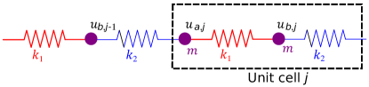
Figure 12: Unit cell of an infinite spring mass chain having alternating spring stiffness $k_{1}$ and $k_{2}$.

We consider a spring mass chain with springs of alternating stiffness $k_{1}$ and $k_{2}$ connecting identical masses as illustrated in Fig. 12. The unit cell is chosen as shown by the dashed box in Fig. 12 To normalize the governing equations, we express the spring stiffness as $k_{1}=k(1+\gamma)$ and $k_{2}=k(1-\gamma)$. Introducing non-dimensional time scale $\tau=t\sqrt{k/m}$, the governing equations for the masses in a unit cell may be expressed in non-dimensional form as

$$\ddot{u}_{a,j}+2u_{a,j}-(1+\gamma)u_{b,j}-(1-\gamma)u_{b,j-1}=0,$$

$$\ddot{u}_{b,j}+2u_{b,j}-(1+\gamma)u_{a,j}-(1-\gamma)u_{a,j+1}=0.$$

We first study the dynamic behavior of the lattice using a dispersion analysis. Imposing a plane wave solution of the form ${\bm{u}}_{j}=(u_{a,j},u_{b,j})=\bm{A}(\mu)e^{i\Omega\tau+i\mu j}$ where $\Omega$ is the frequency and $\mu$ is the non-dimensional wavenumber leads to the following eigenvalue problem

$$\begin{pmatrix}2-\Omega^{2}&-(1+\gamma)-(1-\gamma)e^{-i\mu}\\ -(1+\gamma)-(1-\gamma)e^{i\mu}&2-\Omega^{2}\end{pmatrix}\begin{pmatrix}A_{a}\\ A_{b}\end{pmatrix}\\ =\Omega^{2}\begin{pmatrix}A_{a}\\ A_{b}\end{pmatrix}.$$ (25)

The eigenvalues lead to two branches with frequencies $\Omega=\sqrt{2\pm\sqrt{2+2\gamma^{2}+2(1-\gamma^{2})\cos{\mu}}}$, with the minus and plus signs for the acoustic and optical bands, respectively. The lattice has a bandgap over the frequency range $\Omega\in\left(\sqrt{2(1-|\gamma|)},\sqrt{2(1+|\gamma|)}\right)$.

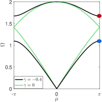
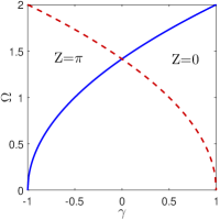
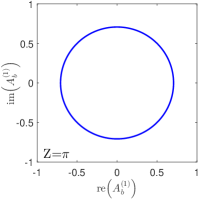
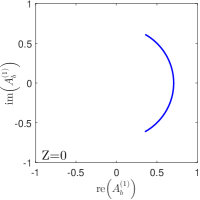
Figure 13: (a) Dispersion relations for lattices with $\gamma=0$ (dotted) and $\gamma=-0.5$ (solid). (b) Limits of the bandgap showing band inversion as $\gamma$ varies. Component $2$ of eigenvector $\bm{A}^{(1)}(\mu)$ as $\mu$ varies from $-\pi$ to $\pi$. (c) $\gamma=-0.5$ has a Zak phase $\pi$ while (d) $\gamma=0.5$ has a zero Zak phase.

Figure 13 displays the dispersion diagrams for stiffness parameters $\gamma=0$ (green dotted curves) and $\gamma=0.4$ (black solid curves). Figure 13 displays the frequencies bounding the bandgap between the acoustic and optical branches as the stiffness parameter $\gamma$ varies. Note that these bounding frequencies are at the wavenumber $\mu=\pi$. The frequency on the dashed (red) curve has an eigenvector $(A_{a},A_{b})=(1/\sqrt{2},\;1/\sqrt{2})^{T}$ while that on the solid (blue) curve has an eigenvector $(1/\sqrt{2},\;-1/\sqrt{2})^{T}$ for all nonzero $\gamma$ values. Note that the modes get inverted, i.e., the antisymmetric $(1/\sqrt{2},\;-1/\sqrt{2})^{T}$ mode has a higher frequency than the symmetric $(1/\sqrt{2},\;1/\sqrt{2})^{T}$ mode as $\gamma$ increases beyond zero. This phenomenon is called band inversion and has been previously exploited in electronic systems Hasan2010 ; Bernevig2006 ; Pankratov1987 and continuous acoustic ones xiao2015geometric to obtain localized modes. These modes are localized at the interface of two lattices: one with $\gamma>0$ and the other with $\gamma<0$.

To further shed light on the topological properties of the eigensolutions, we examine the eigenvectors of lattices with $\gamma>0$ and $\gamma<0$. In particular, we study how they vary with wavenumber $\mu$ over the first Brillouin zone. Observe that the matrix in Eqn. (25) gives the same eigenvalues under the transformation $\gamma\to-\gamma$ but the eigenvectors are different. Indeed, note that the transformation $\gamma\to-\gamma$ may be achieved by simply reversing the direction of the lattice basis vector. An alternate way is to simply translate the unit cell by one mass to the right or left and relabel the masses appropriately. Both these changes correspond to changes in gauge and they change the eigenvectors, thereby changing the topology of the vector bundle associated with the solution of the above eigenvalue problem. We characterize the topology of this vector bundle using the Zak phase zak1989berry for the bands. This quantity is a special case of Berry phase zak1989berry ; xiao2015geometric to characterize the band topology in $1D$ periodic media. It is given for the band $m$ by

$$Z=\int_{-\pi}^{\pi}\left[i(\bm{A}^{(m)})^{H}(\mu)\cdot\partial_{\mu}\bm{A}^{(m)}(\mu)\right]d\kappa,$$ (26)

where $(\bm{A}^{(m)})^{H}(\mu)$ is the conjugate transpose or Hermitian of the eigenvector $\bm{A}^{(m)}(\mu)$. For numerical calculations, we use an equivalent discretized form of Eqn. (26) given by xiao2015geometric

$$\theta^{Zak}=-\textrm{Im}\sum_{n=-N}^{N-1}\ln\left[\bm{A}_{m}^{H}\left({\frac{n}{N}\pi}\right)\cdot\bm{A}_{m}\left({\frac{n+1}{N}\pi}\right)\right].$$ (27)

The Zak phase of both the acoustic and optical bands takes the values $Z=0$ and $Z=\pi$ for the lattices with $\gamma>0$ and $\gamma<0$, respectively. Indeed, it should be noted that since the Zak phase is not gauge invariant atala2013direct , the choice of coordinate reference and unit cell must remain the same for computing this quantity.

To understand the meaning of the Zak phase, we show the behavior of the acoustic mode eigenvector for both $\gamma>0$ and $\gamma<0$ lattices. For consistent representation, a gauge is fixed such that the eigenvector has magnitude $1$ and its first component is real and positive, i.e., at zero angle in the complex plane. The second component $A_{b}^{(1)}$ of the eigenvector is displayed in the complex plane for $\mu$ varying from $-\pi$ to $\pi$, see Figs. 13 and 13. This component of the eigenvector will form a loop as the wavenumber $\mu$ is varied from $-\pi$ to $\pi$. When $\gamma>0$, this eigenvector loop does not enclose the origin and it leads to a Zak phase equal to $0$. On the other hand, the acoustic band of a lattice with $\gamma<0$ has a Zak phase of $Z=\pi$ and its eigenvector loop $A_{b}(\mu)$ encloses the origin.

Appendix C Effective stiffness of interface mass

We consider a finite lattice with an interface and where the masses at both ends are fixed. Using the transfer matrix relations, we derived the following expression in Sec. A for the equivalent stiffness of the interface mass

$$\left[2(1+\gamma)\left(1-\dfrac{S_{21}}{S_{11}}\right)-\Omega^{2}\right]u_{c,0}=f,$$

where $\bm{S}=\bm{T}^{-N}$. Let us now derive an explicit expression for the terms of the matrix $\bm{S}$ which appear in the above expression. Let us assume that $\bm{T}^{-1}$ is diagonalizable. This assumption is verified later by examining its eigenvectors. We now use the following result from linear algebra hoffmanlinear : there exists a unique decomposition $\bm{T}^{-1}=\bm{U}\bm{D}\bm{U}^{-1}$, where $\bm{D}$ is a diagonal matrix having the eigenvalues of $\bm{T}^{-1}$ and $\bm{U}$ is a matrix whose columns are the corresponding eigenvectors of $\bm{T}^{-1}$. We determine this decomposition by solving for the eigenvectors of $\bm{T}^{-1}$, which then leads to the following expression for $\bm{S}$

$$\bm{S} =\bm{T}^{-N}=\bm{U}\bm{D}^{N}\bm{U}^{-1}=[\bm{U}]\begin{pmatrix}\lambda_{1}^{N}&0\\ 0&\lambda_{2}^{N}\end{pmatrix}[\bm{U}^{-1}],$$ (28)

where

$$\lambda_{1,2}=\dfrac{-2-2\gamma^{2}+(2-\Omega^{2})^{2}\pm\Omega\sqrt{(\Omega^{2}-4)(-4\gamma^{2}+(2-\Omega^{2})^{2})}}{2(1-\gamma^{2})},$$

$$[\bm{U}]=\begin{pmatrix}\dfrac{4\gamma+(2-\Omega^{2})^{2}+\Omega\sqrt{(\Omega^{2}-4)(-4\gamma^{2}+(2-\Omega^{2})^{2})}}{2(1+\gamma)(2-\Omega^{2})}&\dfrac{4\gamma+(2-\Omega^{2})^{2}-\Omega\sqrt{(\Omega^{2}-4)(-4\gamma^{2}+(2-\Omega^{2})^{2})}}{2(1+\gamma)(2-\Omega^{2})}\\ 1&1\end{pmatrix}.$$

Note that the term within the square root in the eigenvectors is positive for all frequencies $\Omega$ in the bandgaps and thus the two eigenvectors are distinct. These two distinct eigenvectors span the vector space $\mathbb{R}^{2}$ and hence $\bm{T}^{-1}$ is diagonalizable hoffmanlinear , which verifies the assertion made earlier.

Appendix D Asymptotic analysis procedure

To seek the dispersion relation of the lattice, the governing equation for a lattice unit cell $j$ are written in matrix form as

$$\bm{M}\ddot{\bm{u}}_{j}+\sum_{p}\bm{K}_{p}\bm{u}_{p}+f_{NL}\left(\bm{u}_{j},\bm{u}_{p}\right)=\bm{0}.$$ (29)

The displacement and frequency are solved using the method of multiple scales, having the following asymptotic expansions for displacement $\bm{u}$ and time $t$

$$\bar{\bm{u}}_{j}=\bm{u}_{j}^{(0)}+\epsilon\bm{u}_{j}^{(1)}+O(\epsilon^{2}),\;\;t=\omega\tau=(\omega_{0}+\epsilon\omega_{1}+O(\epsilon^{2}))\tau.$$ (30)

Assuming $\bm{u}_{j}$ is harmonic with frequency $\omega$, and substituting the above equations into the governing equations (Newton’s laws) yields the following equations for the various orders of $\epsilon$:

$$\epsilon^{0}:\;\;\omega_{0}^{2}\bm{M}\dfrac{d^{2}\bm{u}^{(0)}_{m}}{d\tau^{2}}+\sum_{p}\bm{K}_{p}\bm{u}^{(0)}_{m+p}=0,$$ (31)

$$\epsilon^{1}:\;\;\omega^{2}_{0}\bm{M}\dfrac{d^{2}\bm{u}^{(1)}_{m}}{d\tau^{2}}+\sum_{p}\bm{K}_{p}\bm{u}_{m+p}^{(1)}=-2\omega_{0}\omega_{1}\bm{M}\dfrac{d^{2}\bm{u}_{m}^{(0)}}{d\tau^{2}}$$

$$\qquad\qquad\qquad\qquad\qquad-\sum_{p}f_{NL}\left(\bm{u}^{(0)}_{m},\bm{u}^{(0)}_{m+p}\right).$$ (32)

The solution of the above equations yields the first order plane waves and their amplitude dependent dispersion relations.

The zeroth order equation is linear and is solved using the Floquet Bloch theory. We impose a traveling wave solution of the form $\bm{u}^{(0)}_{p}(\tau)=\bm{z}_{m}e^{i\bm{\mu}\cdot\bm{x}_{p}}e^{i\tau}$, where $\bm{z}$ is the eigenvector associated with a wave with wavevector $\bm{\mu}$, $\bm{x}_{p}$ is the spatial location of the center of a unit cell with index $p$ and $\bm{u}^{(0)}_{p}$ is the vector with components having the generalized displacement of unit cell $p$. Substituting this expression into the system of governing equations for a unit cell in Eqn. (31) leads to the eigenvalue problem $\sum_{p}\bm{K}_{p}e^{i\bm{\mu}\cdot\bm{x}_{p}}\bm{z}=\omega_{0}^{2}\bm{M}\bm{z}$ for a fixed wavevector $\bm{\mu}$ in the reciprocal lattice space. Its solution yields the dispersion surface $\omega=\omega(\bm{\mu})$ of the zeroth order linear system. Then the zeroth order displacement of a cell $p$ due to the $m$-th wave mode, with eigenvector $\bm{z}_{m}$, may be written as

$$\bm{u}^{(0)}_{p}(\tau)=\dfrac{A_{0}}{2}\left(\bm{z}_{m}(\bm{\mu})e^{i\bm{\mu}\cdot\bm{x}_{p}}e^{i\tau}+c.c.\right),$$ (33)

where $c.c.$ denotes the complex conjugate, $A_{0}$ is the wave amplitude and $\bm{z}_{m}(\bm{\mu})$ is the $m$-th wave mode at the wavevector $\bm{\mu}$. The eigenvector ${\bm{z}_{m}}(\bm{\mu})$ is normalized so that the maximum absolute value of any component is $1$. Thus the maximum displacement of any mass in the lattice is $A_{0}$.

In contrast with linear media, the dispersion behavior of our nonlinear lattice will depend on the amplitude $A_{0}$ of the wave mode and we determine the first order correction in the dispersion relation as a function of this amplitude. To this end, the first order equation is solved to get a correction due to the nonlinear terms. Substituting Eqn. (33) into the first order equation Eqn. (31) leads to the following equation corresponding to the $j$-th wave mode

$$\omega_{0}^{2}\bm{M}\dfrac{d^{2}\bm{u}^{(1)}_{m}}{d\tau^{2}}+\sum_{p}\bm{K}_{p,m}\bm{u}_{p+m}^{(1)}=\omega_{0}\omega_{1}A_{0}\bm{M}\bm{u}^{(0)}_{m}e^{i\tau}\\ -\sum_{p}f_{NL}(\bm{u}_{m}^{(0)},\bm{u}^{(0)}_{m+p})=\bm{F}(\bm{\mu}).$$ (34)

Note that the linear part of Eqn. (34) (terms on the left) is identical to the $\epsilon^{0}$ order equation (Eqn. (31)). The term $\bm{F}(\bm{\mu})$ on the right hand side is the additional forcing term in the $\epsilon^{1}$ order equation due to nonlinear effects. The component of $\bm{F}$ along $\bm{u}^{0}_{j}$ is identified as a secular term and it should vanish for the $\epsilon^{1}$ solution to be bounded. This condition may be written as

$$\left(\bm{u}^{0}_{j},\bm{F}(\bm{\mu})\right)=\int_{0}^{2\pi}(\bm{u}^{0}_{j})^{H}\bm{F}(\bm{\mu})d\tau=0.$$ (35)

Substituting terms from Eqn. (34) into $\bm{F}$, the above condition leads to an equation for the first order frequency correction $\omega_{1}$. For the $j$-th mode, solving this equation gives

$$\omega_{1}(A_{0},\bm{\mu})=\dfrac{{\bm{u}^{(0)H}_{m}}}{2\pi\omega_{0,j}A_{0}{\bm{u}^{(0)H}_{m}}\bm{M}{\bm{u}^{(0)}_{m}}}\int_{0}^{2\pi}\sum_{p}f_{NL}e^{-i\tau}d\tau.$$ (36)

Note that since $\bm{u}^{(0)}$ is a periodic function of time $\tau$ with period $2\pi$, the nonlinear forcing function $f_{NL}$ is also periodic in $\tau$. The nonlinear forces also depend on the amplitude $A_{0}$ of the zeroth order wave mode.

We now address two technical points which ensure uniqueness of the above expression for $\omega_{1,j}$. The first one is when there are repeated eigenvalues and the second one is about the invariance of the correction $\omega_{1}$ to the scaling of eigenvectors by $e^{i\theta}$. A procedure is outlined to address the case of repeated eigenvalues in a systematic way which results in a unique and well defined value of the frequency correction. Let us consider a wavevector $\bm{\mu}$ at which there are $p$ repeated eigenvalues $\omega_{0}$ and the corresponding eigenvectors are $\{\bm{v}_{i}:1\leq i\leq p\}$. A linear combination of any of these $p$ eigenvectors is also a valid eigenvector and these eigenvectors define a vector subspace. However, note that $\bm{c}_{1}$ in Eqn. (36) depends on the eigenvectors in a nonlinear way and hence its value will depend on the choice of eigenvectors from this vector subspace. As an illustrative example, consider the eigenvalues and eigenvectors of the identity $\bm{I}_{2}$ matrix. It has a repeated eigenvalue $1$ and the corresponding eigenvectors are non-unique. We consider two sets of eigenvectors $(\bm{v}_{1},\bm{v}_{2})$ and $(\bm{w}_{1},\bm{w}_{2})$:

$$\bm{v}_{1}=\begin{pmatrix}1\\ 0\end{pmatrix}e^{i\tau},\;\;\bm{v}_{2}=\begin{pmatrix}0\\ 1\end{pmatrix}e^{i\tau},$$

$$\bm{w}_{1}=\begin{pmatrix}1/\sqrt{2}\\ 1/\sqrt{2}\end{pmatrix}e^{i\tau},\;\;\bm{w}_{2}=\begin{pmatrix}1/\sqrt{2}\\ -1/\sqrt{2}\end{pmatrix}e^{i\tau}.$$

Solving for $\omega_{1}$ gives different values for the $\bm{v}_{i}$ and $\bm{w}_{i}$ sets as $\bm{c}_{1}$ has a nonlinear dependence on the components. To resolve this anomaly, we remark here that the eigenvalue correction corresponds to waves propagating at specific prescribed amplitude $A_{0}$. Note that this amplitude is prescribed on distinct eigenvectors in a mutually exclusive manner. For example, if we prescribe the zeroth order solution displacement on masses $(i,j)$, the eigenvectors $(\bm{u}_{1},\bm{u}_{2})$ having common eigenvalue should satisfy the constraint

$$v_{1}(i)=\alpha A_{0},\;\;v_{1}(j)=0,\;\;\;v_{2}(i)=0,\;\;v_{2}(j)=\beta A_{0},\;\;\;$$ (37)

where $\alpha$ and $\beta$ are normalizing constants such that the maximum magnitude of any component is unity (i.e., $\|\bm{v}_{1}\|_{\infty}=\|\bm{v}_{2}\|_{\infty}=1$).

Extending the above observation to the general case having $p$ common eigenvalues with eigenvectors, we present the following approach to get a set of transformed eigenvectors which obey a generalized form of the constraint in Eqn. (37). For each eigenvector $\bm{u}_{i}$ in this set of repeated eigenvalues, we find a corresponding transformed eigenvector $\bm{v}_{i}$ by setting $p-1$ components of $\bm{u}_{i}$ to zero. These $p-1$ components are simply chosen to be those which have the highest magnitude. Note that if the indices of these components coincide with those chosen for another $i$ distinct from this set of repeated of repeated eigenvalues, then a different set of indices are chosen. This procedure ensures that we are enforcing distinct components to zero value to get the orthogonal modes.

The second point about the invariance of $\omega_{1,j}$ to the specific choice of gauge factor $e^{i\theta}$ is explained by noting that only the component corresponding to $e^{i\tau}$ in $f_{NL}$ is relevant to the computation of $\bm{c}_{1}$ and the contribution of all other components is zero due to orthogonality. Hence, $\bm{c}_{1}$ depends linearly on $e^{i\theta}$ and multiplying by $\bm{u}^{H}$, which has a factor $e^{-i\theta}$ ensures that the resulting final expression is independent of $\theta$.

References

- [1] MI Hussein, MJ Leamy, and M Ruzzene. Dynamics of phononic materials and structures: Historical origins, recent progress, and future outlook. Applied Mechanics Reviews, 66(4):040802, 2014.
- [2] SD Huber. Topological mechanics. Nature Physics, 12(7):621–623, 2016.
- [3] C Brendel, V Peano, O Painter, and F Marquardt. Snowflake topological insulator for sound waves. arXiv preprint arXiv:1701.06330, 2017.
- [4] Alexander B Khanikaev, S Hossein Mousavi, Wang-Kong Tse, Mehdi Kargarian, Allan H MacDonald, and Gennady Shvets. Photonic topological insulators. Nature materials, 12(3):233–239, 2013.
- [5] V Peano, C Brendel, M Schmidt, and F Marquardt. Topological phases of sound and light. arXiv preprint arXiv:1409.5375, 2014.
- [6] SH Mousavi, AB Khanikaev, and Z Wang. Topologically protected elastic waves in phononic metamaterials. Nature communications, 6, 2015.
- [7] Raj Kumar Pal and Massimo Ruzzene. Edge waves in plates with resonators: an elastic analogue of the quantum valley hall effect. New Journal of Physics, 19(2):025001, 2017.
- [8] N Swinteck, S Matsuo, K Runge, JO Vasseur, P Lucas, and PA Deymier. Bulk elastic waves with unidirectional backscattering-immune topological states in a time-dependent superlattice. Journal of Applied Physics, 118(6):063103, 2015.
- [9] H Nassar, XC Xu, AN Norris, and GL Huang. Modulated phononic crystals: Non-reciprocal wave propagation and willis materials. Journal of the Mechanics and Physics of Solids, 101:10–29, 2017.
- [10] E Prodan and C Prodan. Topological phonon modes and their role in dynamic instability of microtubules. Physical review letters, 103(24):248101, 2009.
- [11] LM Nash, D Kleckner, A Read, V Vitelli, AM Turner, and WTM Irvine. Topological mechanics of gyroscopic metamaterials. Proceedings of the National Academy of Sciences, 112(47):14495–14500, 2015.
- [12] AB Khanikaev, R Fleury, SH Mousavi, and A Alù. Topologically robust sound propagation in an angular-momentum-biased graphene-like resonator lattice. Nature communications, 6, 2015.
- [13] RK Pal, M Schaeffer, and M Ruzzene. Helical edge states and topological phase transitions in phononic systems using bi-layered lattices. Journal of Applied Physics, 119(8):084305, 2016.
- [14] C He, Z Li, X Ni, XC Sun, SY Yu, MH Lu, XP Liu, and YF Chen. Topological phononic states of underwater sound based on coupled ring resonators. Applied Physics Letters, 108(3):031904, 2016.
- [15] R Süsstrunk and SD Huber. Observation of phononic helical edge states in a mechanical topological insulator. Science, 349(6243):47–50, 2015.
- [16] J Ningyuan, C Owens, A Sommer, D Schuster, and J Simon. Time-and site-resolved dynamics in a topological circuit. Physical Review X, 5(2):021031, 2015.
- [17] E Prodan, K Dobiszewski, A Kanwal, J Palmieri, and C Prodan. Dynamical majorana edge modes in a broad class of topological mechanical systems. Nature Communications, 8:14587, 2017.
- [18] R Chaunsali, A Thakkar, E Kim, PG Kevrekidis, and J Yang. Demonstrating an in-situ topological band transition in cylindrical granular chains. arXiv preprint arXiv:1702.04756, 2017.
- [19] M Xiao, G Ma, Z Yang, P Sheng, ZQ Zhang, and CT Chan. Geometric phase and band inversion in periodic acoustic systems. Nature Physics, 11(3):240–244, 2015.
- [20] CL Kane and TC Lubensky. Topological boundary modes in isostatic lattices. Nature Physics, 10(1):39–45, 2014.
- [21] J Paulose, AS Meeussen, and V Vitelli. Selective buckling via states of self-stress in topological metamaterials. Proceedings of the National Academy of Sciences, 112(25):7639–7644, 2015.
- [22] DZ Rocklin, BG Chen, M Falk, V Vitelli, and TC Lubensky. Mechanical weyl modes in topological maxwell lattices. Physical review letters, 116(13):135503, 2016.
- [23] D Rocklin. Directional mechanical response in the bulk of topological metamaterials. arXiv preprint arXiv:1612.00084, 2016.
- [24] R Fleury, DL Sounas, CF Sieck, MR Haberman, and A Alù. Sound isolation and giant linear nonreciprocity in a compact acoustic circulator. Science, 343(6170):516–519, 2014.
- [25] J Vila, RK Pal, M Ruzzene, and G Trainiti. A bloch-based procedure for dispersion analysis of lattices with periodic time-varying properties. arXiv preprint arXiv:1702.01728, 2017.
- [26] RK Pal and PH Geubelle. Wave tailoring by precompression in confined granular systems. Physical Review E, 90(4):042204, 2014.
- [27] N Boechler, G Theocharis, and C Daraio. Bifurcation-based acoustic switching and rectification. Nature materials, 10(9):665–668, 2011.
- [28] Andrea Alù. Metamaterials: Prime time. Nature Materials, 15(12):1229–1231, 2016.
- [29] Y Hadad, AB Khanikaev, and A Alù. Self-induced topological transitions and edge states supported by nonlinear staggered potentials. Physical Review B, 93(15):155112, 2016.
- [30] Mark J Ablowitz, Christopher W Curtis, and Yi-Ping Ma. Linear and nonlinear traveling edge waves in optical honeycomb lattices. Physical Review A, 90(2):023813, 2014.
- [31] Daniel Leykam and Yi Dong Chong. Edge solitons in nonlinear-photonic topological insulators. Physical review letters, 117(14):143901, 2016.
- [32] Yaakov Lumer, Yonatan Plotnik, Mikael C Rechtsman, and Mordechai Segev. Self-localized states in photonic topological insulators. Physical review letters, 111(24):243905, 2013.
- [33] Mark J Ablowitz and Justin T Cole. Tight-binding methods for general longitudinally driven photonic lattices: Edge states and solitons. Physical Review A, 96(4):043868, 2017.
- [34] Xin Zhou, You Wang, Daniel Leykam, and YD Chong. Optical isolation with nonlinear topological photonics. arXiv preprint arXiv:1705.06921, 2017.
- [35] RK Narisetti, MJ Leamy, and M Ruzzene. A perturbation approach for predicting wave propagation in one-dimensional nonlinear periodic structures. Journal of Vibration and Acoustics, 132(3):031001, 2010.
- [36] RK Narisetti, M Ruzzene, and MJ Leamy. A perturbation approach for analyzing dispersion and group velocities in two-dimensional nonlinear periodic lattices. Journal of Vibration and Acoustics, 133(6):061020, 2011.
- [37] Meng Xiao, ZQ Zhang, and Che Ting Chan. Surface impedance and bulk band geometric phases in one-dimensional systems. Physical Review X, 4(2):021017, 2014.
- [38] AH Nayfeh. Perturbation methods. John Wiley & Sons, 2008.
- [39] L Verlet. Computer ”experiments” on classical fluids. i. thermodynamical properties of lennard-jones molecules. Phys. Rev., 159:98–103, 1967.
- [40] MZ Hasan and CL Kane. Colloquium: topological insulators. Reviews of Modern Physics, 82(4):3045, 2010.
- [41] MZ Hasan and CL Kane. Colloquium : Topological insulators. Rev. Mod. Phys., 82:3045–3067, 2010.
- [42] BA Bernevig, TL Hughes, and SC Zhang. Quantum spin hall effect and topological phase transition in hgte quantum wells. Science, 314(5806):1757–1761, 2006.
- [43] OA Pankratov, SV Pakhomov, and BA Volkov. Supersymmetry in heterojunctions: Band-inverting contact on the basis of Pb1xSnxTe and Hg1xCdxTe. Solid State Communications, 61(2):93 – 96, 1987.
- [44] J Zak. Berry’s phase for energy bands in solids. Physical review letters, 62(23):2747, 1989.
- [45] M Atala, M Aidelsburger, JT Barreiro, D Abanin, T Kitagawa, E Demler, and I Bloch. Direct measurement of the zak phase in topological bloch bands. Nature Physics, 9(12):795–800, 2013.
- [46] K Hoffman and R Kunze. Linear algebra. 1971. Englewood Cliffs, New Jersey.