On a representation of fractional Brownian motion and the limit distributions of statistics arising in cusp statistical models

Abstract. We discuss some extensions of results from the recent paper by Chernoyarov et al. (Ann. Inst. Stat. Math., October 2016) concerning limit distributions of Bayesian and maximum likelihood estimators in ”signal plus white noise” model with irregular cusp-type signals. Using a new representation of fractional Brownian motion (fBm) in terms of cusp functions we show that, as the noise intensity tends to zero, the limit distributions can be expressed in terms of fBm for the full range of asymmetric cusp-type signals correspondingly with the Hurst parameter $H$, $0<H<1$. The  simulation results for the densities and variances of the limit distributions of Bayesian and maximum likelihood estimators are also provided.

1. Introduction and main results. The monograph of Ibragimov and Khasminskii [10] contains a powerful technique for studying asymptotic properties of Bayesian estimators (BE) $\tilde{\theta}_{n}$ and maximum likelihood estimators (MLE) $\hat{\theta}_{n}$ of a parameter $\theta~{}\$based on independent identically distributed (i.i.d.) observations $X^{n}=\left(X_{1},\ldots,X_{n}\right)\$with the marginal density function $f\left(x,\theta\right)$. In particular, for irregular statistical models they showed (see [10], Chapter 6, Theorem 6.2 and Theorem 6.4 ) that the limit distributions of $\ \tilde{\theta}_{n}$ and$~{}\hat{\theta}_{n}$, as$\ \ n\rightarrow\infty$, can be represented using Poisson or Gaussian processes which in their turn are defined in terms of the singularity points of a density function. The particular case of cusp-type densities

$$f\left(x,\theta\right)={h(x,}{\theta)}\exp\left\{-g(x,\theta)|x-\theta|^{\alpha}\right\},~{}\theta\in\Theta=(\theta_{1},\theta_{2}),~{}x\in R=(-\infty,\infty),$$ (1)

where $\alpha>0,~{}h~{}$and $g~{}$are smooth functions, was discussed in the original paper [11], see also Chapter 6 in [10].

The question about efficiency of MLE in irregular i.i.d. statistical experiments, in particular, with $\alpha>\frac{1}{2}$ in (1) was raised by H. Daniels [3] who showed that the MLE is asymptotically efficient and normal in this case. Subsequently, P. Rao [23] showed that the limit distribution of $\hat{\theta}_{n}$ for $\alpha\in(0,1/2)~{}$can be expressed in terms of fractional Brownian motion (fBm) with the Hurst parameter $H=\alpha+1/2\in(1/2,1)$ although the question about its efficiency had not been addressed in [23].

Recall that continuous Gaussian process $W^{H}=\{W_{u}^{H},u\in R\}~{}$with$\,W_{0}^{H}=0,\ E(W_{u}^{H})=0$ is said to be a standard fBm with the Hurst parameter $\,H\in(0,1]\$if

$$\,E|W_{u}^{H}-W_{s}^{H}|^{2}=|u-s|^{2H},\,\ u\in R,~{}s\in R.$$ (2)

A standard two-sided Brownian motion $W=(W_{u}^{1/2},~{}u\in R)$ is a particular case of this definition.

Further we use the following notations:

$$L(\theta,X^{n}):=\prod\limits_{i=1}^{n}f\left(X_{i},\theta\right)$$

for the likelihood function;

$$\tilde{\theta}_{n}=\frac{\int_{{}_{{}_{-\infty}}}^{{}^{{}^{\infty}}}u\,L(u,X^{n})q(u)du}{\int_{{}_{{}_{-\infty}}}^{{}^{{}^{\infty}}}\,L(u,X^{n})q(u)du}$$

for the BE with respect to quadratic loss function and the prior distribution $q(\theta)$.

Set

$$Z_{u}^{(H)}:=\exp\{W_{u}^{H}-\frac{|u|^{2H}}{2}\},~{}u\in R.$$

Under some mild assumptions on $q(\theta)$ (including the case $q(\theta)=1~{}$i.e. Pitman-type estimators, see [22]) the theory developed in [10] implies the following result for the i.i.d. cusp model (1) with $\alpha\in(0,1/2),~{}H=\alpha+1/2$:

$$(\tilde{\theta}_{n}-\theta)n^{{}^{\frac{1}{2H}}}/C_{H}\overset{d}{\longrightarrow}\zeta_{H}:=\frac{\int_{{}_{{}_{-\infty}}}^{{}^{{}^{\infty}}}uZ_{u}^{(H)}du}{\int_{{}_{{}_{-\infty}}}^{{}^{{}^{\infty}}}Z_{u}^{(H)}du},$$ (3)

where $C_{H}$ is a known constant, the convergence $\overset{d}{\longrightarrow}$ is understood in distribution.

Furthermore, for MLE $\hat{\theta}_{n}$ it was shown in [23] that

$$(\hat{\theta}_{n}-\theta)n^{{}^{\frac{1}{2H}}}/C_{H}\overset{d}{\longrightarrow}\xi_{H}:=\arg\max_{u\in R}(Z_{u}^{(H)}).$$ (4)

Hence, both BE $\tilde{\theta}_{n}$ and MLE $\hat{\theta}_{n}$ have the same rate of convergence $n^{{}^{-\frac{1}{2H}}},~{}H\in(1/2,1)$ for the i.i.d. cusp model (1). Note that some general properties of $\zeta_{H},\ H\in(0,1),$ have been studied in [18], [19] where, in particular, the positive finite constant $\lambda_{H}$  found is such that for all $\lambda<\lambda_{H}$

$$E\exp\{\lambda|\zeta_{H}|^{2H}\}<\infty$$

implying finiteness of the moments of $|\zeta_{H}|.$

In a similar context other continuous and discrete time models with fBm $W^{H}$ arising in the limits have been discussed in the monograph by Kutoyants [15], Dachian [4], Gushchin and Küchler [9], Döring [6] and the references therein. The only paper, where the limits similar to (3) and (4) appear with $H\in(0,\frac{1}{2})$, is [8], where an observed diffusion process had the drift of the form $a|X_{t}-\theta|^{\alpha}$. Note that in [8] it is assumed that the observed diffusion process is a weak solution of the stochastic differential equation; however, for defining of the likelihood ratio process the existence of a strong solution is required and this fact had not been addressed.

In engineering and statistical literature there is a great interest to the ”signal plus white noise” type models, where observations $X^{T}=\left(X_{t},0\leq t\leq T\right)\$have the following dynamics

$$dX_{t}=S(t,\theta)dt+\varepsilon dw_{t},\quad X_{0}=0,\quad 0\leq t\leq T,~{}\varepsilon>0,~{}0<\theta_{1}<\theta<\theta_{2}<T.$$ (5)

Here we assume that $w=\{w_{t},\ 0\leq t\leq T\}$ is a standard one-sided Brownian motion, $S(t,\theta)$ is a ”deterministic signal” which depends on a parameter $\theta$  to be estimated, the “finite energy” condition

$$\int_{0}^{T}S^{2}(u,\theta)du<\infty$$ (6)

holds and $T$ is fixed. The important scenario “large signal-to-noise ratio” corresponds to $\varepsilon\rightarrow 0$.

The case of the observations $X^{nT}=\left(X_{t},~{}0\leq t\leq nT\right)$ of  $T$-periodic signal $S(t,\theta)$ with $\varepsilon=1,~{}n=1,...,$ in (5) can be reduced to this model with $\varepsilon=\frac{1}{\sqrt{n}},~{}X^{T}=\left(X_{t},\ 0\leq t\leq T\right)$ if we put

$$X_{t}=\frac{1}{n}\sum_{j=1}^{n}\left(X_{T\left(j-1\right)+t}-X_{T\left(j-1\right)}\right),\ 0\leq t\leq T.$$

The model (5) is very different from (1), however, Chernoyarov et al. [2] showed that for cusp-type signals of the form

$$S(t,\theta)=a|t-\theta|^{\alpha},\ \alpha\in(0,\frac{1}{2}),$$ (7)

the limit distributions of BE $\tilde{\theta}_{\varepsilon}$ and MLE $\hat{\theta}_{n}$ are also expressed in terms of fBm with  $H=\alpha+1/2\in(1/2,1)$.

One of the main results of our paper is the extension of results of [2] for model (5) to the case $H\in(0,1)$ under more general assumptions, namely, when “signal” might be the asymmetric cusp function of the following form

$$S(t,\theta)=q_{\alpha}(t-\theta)+h(t,\theta),$$ (8)

$$q_{\alpha}(x):=(aI\{x\geq 0\}+bI\{x<0\})|x|^{\alpha},\ \alpha\in(-\frac{1}{2},\frac{1}{2}),\ a\geq 0,\ b\geq 0,\ ab\neq 0,$$ (9)

where $h(t,\theta)\in C^{1,1}$  is a continuously differentiable with respect both $t$ and $\theta,$ $I\{.\}$ is the indicator function. Such signals are unbounded for $\alpha\in(-\frac{1}{2},0);$ however,  condition (6) still holds. In the case of  “discontinuous signals” from (5) with

$$S(t,\theta)=aI\{t-\theta>0\},~{}0\leq t\leq T,$$

as it was shown  in Section 7 of  [10], the asymptotic results of the type (3) and (4) hold with $H=1/2.$

Further we use the following notation with $q_{\alpha}$ from (9) and set

$$\Gamma_{\alpha}^{2}:=\int_{-\infty}^{\infty}(q_{\alpha}(y-1)-q_{\alpha}(y))^{2}dy,~{}\alpha\in(-\frac{1}{2},\frac{1}{2}).$$ (10)

Here and below we consider all stochastic integrals in the Ito’s sense.

The following new representation for fBm will play an important role in finding the limit distributions for the cusp model (5).

Theorem 1. Let $W=(W_{y},\ y\in R)$ be a standard two-sided Bm, $q_{a}(x)$ be the cusp function from (9). Then the process

$$Y_{u}^{H}:=\Gamma_{\alpha}^{-1}\int_{-\infty}^{\infty}(q_{a}(y-u)-q_{a}(y))dW_{y},\ u\in R,~{}\alpha\in(-\frac{1}{2},\frac{1}{2}),~{}H=\alpha+1/2,$$ (11)

is the standard two-sided fBm $W^{H}$.

The proof and references within about other representations for $W^{H}$ can be found in Section 2.

The particular case of (11) with $\alpha\in(0,\frac{1}{2})$ and $a=b~{}$was noted in [20], however, to the best of our knowledge the case $\alpha\in(-\frac{1}{2},0)~{}$for the cusp signal has not been explored so far and this paper fills the gap in the existing theory.

Further we discuss the model (5) with the signal of the form (8) and prove the asymptotic results extending the aforementioned results from [2] to the case $H=\alpha+\frac{1}{2}\in(0,1)$.

We denote the likelihood ratio (i.e. the Radon-Nykodim density, expressed in terms of $X$, [10]) as

$$L(\theta,X^{T}):=\exp\{\frac{1}{\varepsilon^{2}}\int_{0}^{T}S(t,\theta)dX_{t}-\frac{1}{2\varepsilon^{2}}\int_{0}^{T}(S(t,\theta))^{2}dt\}$$ (12)

Our next main result is about the limit distributions for MLE $\hat{\theta}_{n}~{}$ (12) and general BE $\tilde{\theta}_{\varepsilon}^{.}$, under the assumption that the prior $q(\theta),~{}\theta\in\Theta=(\theta_{1},\theta_{2})~{}$ is a continuous positive function, including the Pitman-type estimate with noninformative prior

$$\tilde{\theta}_{\varepsilon}^{P}=\frac{\int_{{}_{{}_{\theta_{1}}}}^{\theta_{2}}u\,L(u,X^{T})du}{\int_{{}_{{}_{\theta_{1}}}}^{\theta_{2}}\,L(u,X^{T})du}.$$

For emphasising the dependence of the expected values and distributions on an unknown parameter $\theta\$below  we will use the notation $\mathbf{E}_{\theta}\left(.\right)$ and $P_{\theta}^{.}(.).$

Theorem 2. Let (5) the cusp signal be defined as (8) with (9) such that $\alpha\in(-1/2,1/2),$ $H=\alpha+1/2\in(0,1)$. Then as $\varepsilon\rightarrow 0$

$$\frac{(\hat{\theta}_{\varepsilon}-\theta)}{(\varepsilon/\Gamma_{\alpha})^{\frac{1}{H}}}\overset{d}{\longrightarrow}\xi_{H},~{}\lim_{\varepsilon\rightarrow 0}\mathbf{E}_{\theta}\left(\frac{\hat{\theta}_{\varepsilon}-\theta}{(\varepsilon/\Gamma_{\alpha})^{\frac{1}{H}}}\right)^{2}=\mathbf{E}\left(\xi_{H}^{2}\right)<\infty,$$ (13)

$$\frac{(\tilde{\theta}_{\varepsilon}-\theta)}{(\varepsilon/\Gamma_{\alpha})^{\frac{1}{H}}}\overset{d}{\longrightarrow}\zeta_{H},~{}\lim_{\varepsilon\rightarrow 0}\mathbf{E}_{\theta}\left(\frac{\tilde{\theta}_{\varepsilon}-\theta}{(\varepsilon/\Gamma_{\alpha})^{\frac{1}{H}}}\right)^{2}=\mathbf{E}\left(\zeta_{H}^{2}\right)<\infty.$$ (14)

Moreover, for any estimator $\theta_{\varepsilon}=\theta_{\varepsilon}(X^{T})$

$$\mathop{\underline{\lim}}\limits_{\delta\rightarrow 0}\mathop{\underline{\lim}}\limits_{\varepsilon\rightarrow 0}\sup_{\left|\theta-\theta_{0}\right|\leq\delta}\mathbf{E}_{\theta}\left(\frac{\theta_{\varepsilon}-\theta}{(\varepsilon/\Gamma_{\alpha})^{\frac{1}{H}}}\right)^{2}\geq\mathbf{E}\left(\zeta_{H}^{2}\right).$$ (15)

The proof of Theorem 2 along with some discussions is presented in Section 3.

According to Theorem 2 both estimators $\hat{\theta}_{\varepsilon}$ and $\tilde{\theta}_{\varepsilon}$ have the same rate of convergence $\varepsilon^{{}^{\frac{1}{H}}}\$which is known to be the best possible rate. It is natural to make a comparison of the properties of these estimators, however, the analytical tools for studying of functionals of fBm are very limited. In Section 4 we have included the series of simulation results to illustrate properties of the limit random variables$~{}\zeta_{H}~{}$and $\xi_{H}~{}\,$for $H\in[0.3,1);$ these results demonstrate that the ratio of variances $\mathbf{E}\left(\xi_{H}^{2}\right)/\mathbf{E}\left(\zeta_{H}^{2}\right)~{}$monotonically decreases from (approximately) $1.4.~{}$to $1$ as $H~{}\$increases from $0.3$ to $1$.

2. Representations of fBm $W^{H},~{}H\in(0,1)$.

One can check (e.g. using Mathematica^@, version 11.0) that $\Gamma_{\alpha}^{2}$  defined in (10) can be expressed in terms of Gamma function $\Gamma[x]~{}$for any$~{}\alpha\in(-\frac{1}{2},0)\cup(\frac{1}{2},1)$

$$\Gamma_{\alpha}^{2}=\frac{\sqrt{\pi}\Gamma[1+\alpha]}{2^{2\alpha+1}\Gamma[3/2+\alpha]}(\sec[\pi\alpha](a^{2}+b^{2})-2ab).$$

For $\alpha\in(0,\frac{1}{2}),\$see other equivalent representations in [23], p. 79 and [10], p. 306.

Proof of Theorem 1. The stochastic process $Y_{u}^{H}$ is an Ito-type integral of a deterministic integrand and, obviously, $Y_{u}^{H}$  is a Gaussian process,  $Y_{0}^{H}=0,\ EY_{u}^{H}=0.~{}$Thus for verifying the statement of Theorem 1 we only need to find $E|Y_{u}^{H}-Y_{s}^{H}|^{2}$ for $u>s.$

Using the isometry property of Ito integrals and then the substitution $y=z+s~{}$ we have

$$E|Y_{u}^{H}-Y_{s}^{H}|^{2} = \Gamma_{\alpha}^{-2}\int_{-\infty}^{\infty}(q_{\alpha}(y-u)-q_{\alpha}(y-s))^{2}dy$$

$$= \Gamma_{\alpha}^{-2}\int_{-\infty}^{\infty}(q_{\alpha}(z-(u-s))-q_{\alpha}(z))^{2}dz.$$

Making the substitution $z=(u-s)x~{}$ and using the identities

$$q_{\alpha}((u-s)x-(u-s))=|u-s|^{\alpha}q_{\alpha}(x-1),~{}q_{\alpha}((u-s)x)=|u-s|^{\alpha}q_{\alpha}(x)$$

we obtain

$$E|Y_{u}^{H}-Y_{s}^{H}|^{2}=\left|u-s\right|^{2\alpha+1}\Gamma_{\alpha}^{-2}\int_{-\infty}^{\infty}(q_{\alpha}(x-1)-q_{\alpha}(x))^{2}dx=\left|u-s\right|^{2H}$$

where $H=\alpha+\frac{1}{2}.~{}$The proof is completed.

Remark 1.

For the symmetric case $a=b$ representation (11) was obtained in [20].

If $~{}a=1,~{}b=0~{}$it is equivalent to the Mandelbrot-Van Ness representation:

$$Y_{u}^{H}=\Gamma_{\alpha}^{-1}(\int_{0}^{u}(u-y)^{\alpha}dW\left(y\right)+\int_{-\infty}^{0}((u-y)^{\alpha}-(-y)^{\alpha})dW\left(y\right)),u\in R,$$

see [16].

The Muravlev’s representation [17] in terms of Ornstein-Uhlenbeck processes is a consequence of the Mandelbrot-Van Ness representation; actually, the latter can be considered as a consequence of Kolmogorov’s representation [13] for fBm in terms of a Fourier transform of a Gaussian random field. There exist other representations for the fBm, not directly connected to (11), see e.g. Norros et al. [21].

Remark 2. Theorem 6.2.1 from [10], applied to a particular case of cusp densities (9), contains a representation for the limit of normalized likelihood ratio process (NLRP) in the form of stochastic integrals of cusp-type functions. Interestingly, the connection of such stochastic processes to the fBm had not been discussed in [10] at all. Now using (11) one can easily check that in [10] the Gaussian component in the limit of NLRP for the case under consideration is nothing else but the fBm $W^{H},~{}H\in(\frac{1}{2},1)$.

3. Cusp-type signals in ”signal plus white noise” model

Further we use the following notation for the NLRP

$$Z_{T}\left(u,\varepsilon\right):=\frac{L(\theta-\varphi_{\varepsilon}u,X^{T})}{L(\theta,X^{T})}$$

$$=\exp\{\varepsilon^{-2}\int_{0}^{T}[S(t,\theta-\varphi_{\varepsilon}u)-S(t,\theta)]dX_{t}-\frac{\varepsilon^{-2}}{2}\int_{0}^{T}(S^{2}(t,\theta-\varphi_{\varepsilon}u)-S^{2}(t,\theta))dt\},$$

where we assume $u\in U_{\varepsilon}:=(\frac{\theta_{1}-\theta}{\varphi_{\varepsilon}},\frac{\theta_{2}-\theta}{\varphi_{\varepsilon}})~{}$and set

$$\varphi_{\varepsilon}:=(\varepsilon/\Gamma_{\alpha})^{\frac{1}{H}},$$

thus $\varepsilon^{-2}\varphi_{\varepsilon}^{2H}\Gamma_{\alpha}^{2}=1$. Having chosen $\varphi_{\varepsilon},$ this way we obtain the representations for the limit distributions of $\hat{\theta}_{\varepsilon}$ and $\tilde{\theta}_{\varepsilon}~{}$identical to these in (3) and (4). The limit distributions in [2] can be transformed to (13) and (14) after properly adjusting the normalising factor $\varphi_{\varepsilon}$.

The proof of Theorem 2 is based on the properties of NLRP $Z_{T}\left(u,\varepsilon\right)$.  First, we prove the convergence of marginal distributions of $Z_{T}\left(u,\varepsilon\right)$ to $Z_{u}^{(H)}=\exp\{W_{u}^{H}-\frac{|u|^{2H}}{2}\}$ as $\varepsilon\rightarrow 0,\ u\in R,~{}$ $H=\alpha+1/2.$

Proposition 1. Assume (5) holds where

$$S(t,\theta)=q_{\alpha}(t-\theta)+h(t,\theta),~{}\alpha\in(-\frac{1}{2},\frac{1}{2}),$$

$h(t,\theta)\in C^{1,1},\,0<\theta_{1}<\theta<\theta_{2}<T.$

Then the marginal distributions of $\{Z_{T}\left(u,\varepsilon\right),\ u\in U_{\varepsilon}\}$ converge to marginal distributions of $\{Z_{u}^{(H)},\ u\in R\},~{}H=\alpha+\frac{1}{2}.$

Proof. Using the equation $dX_{t}=S(t,\theta)dt+\varepsilon dw_{t}$ we have

$$Y_{\varepsilon}(u) : =\log(Z_{T}\left(u,\varepsilon\right))$$

$$= \varepsilon^{-1}\int_{0}^{T}[S(v,\theta-\varphi_{\varepsilon}u)-S(v,\theta)]dw_{v}-\frac{\varepsilon^{-2}}{2}\int_{0}^{T}[S(v,\theta-\varphi_{\varepsilon}u)-S(v,\theta)]^{2}dv$$

$$: =A_{\varepsilon}(u)-B_{\varepsilon}(u).$$

First we show, as $\varepsilon\rightarrow 0,~{}$ the deterministic part of this decomposition

$$B_{\varepsilon}(u)\rightarrow\frac{|u|^{2H}}{2},\ u\in R,$$

and the stochastic integral part

$$E_{\theta}|A_{\varepsilon}(u)-A_{\varepsilon}(s)|^{2}\rightarrow E|W_{u}^{H}-W_{s}^{H}|^{2}=|u-s|^{2H},\,\ u\in R,~{}s\in R.$$

The last convergence is equivalent to the convergence of covariance functions of $A_{\varepsilon}(u)~{}$to $W^{H}~{}$ and since $A_{\varepsilon}(u)$ is a Gaussian process this will imply the result.

We have

$$B_{\varepsilon}(u)=\varepsilon^{-2}\int_{0}^{T}[q_{\alpha}(v-\theta-\varphi_{\varepsilon}u)-q_{\alpha}(v-\theta)+\delta_{\varepsilon}(v,u)]^{2}dv,$$

where

$$\delta_{\varepsilon}(v,u):=h(v,\theta-\varphi_{\varepsilon}u)-h(v,\theta)=\varphi_{\varepsilon}D(v,\theta,u)(1+o(1))=o(\varphi_{\varepsilon}).$$

Since $h(v,\theta)\in C^{1,1}$ one can easily see that the total input of $\delta_{\varepsilon}(t,u)$ to $B_{u}(\varepsilon)$ is of order $o(1)~{}$because

$$\varepsilon^{-2}\int_{0}^{T}(\delta_{\varepsilon}(v,u))^{2}dv\leq\varepsilon^{-2}\varphi_{\varepsilon}^{2}\max_{v}|D(v,\theta,u)|^{2}T$$

and $\varepsilon^{-2}\varphi_{\varepsilon}^{2}=\varepsilon^{-2}\varphi_{\varepsilon}^{2H}\varphi_{\varepsilon}^{2-2H}=o(1)$. Hence, we obtain with the substitution $v=\theta+\varphi_{\varepsilon}t~{}~{}$

$$B_{\varepsilon}(u)=\varepsilon^{-2}\int_{0}^{T}[q_{\alpha}(v-\theta-\varphi_{\varepsilon}u)-q_{\alpha}(v-\theta)]^{2}dv+o(1)$$

$$=\varepsilon^{-2}\varphi_{\varepsilon}^{2\alpha+1}\int_{-\theta/\varphi_{\varepsilon}}^{(T-\theta)/\varphi_{\varepsilon}}[q_{\alpha}(t-u)-q_{\alpha}(t)]^{2}dt+o(1)$$

(recall $\varepsilon^{-2}\varphi_{\varepsilon}^{2\alpha+1}\Gamma_{\alpha}^{2}=1,~{}T>\theta_{2}\geq\theta\geq\theta_{1}>0$)

$$\rightarrow\Gamma_{\alpha}^{-2}\int_{-\infty}^{\infty}[q_{\alpha}(t-u)-q_{\alpha}(t)]^{2}dt=|u|^{2H},\ u\in R.$$

Due to the isometry of stochastic integrals we obtain

$$E_{\theta}|A_{\varepsilon}(u)-A_{\varepsilon}(s)|^{2}$$

$$= \varepsilon^{-2}\int_{0}^{T}[q_{\alpha}(v-\theta-\varphi_{\varepsilon}u)-q_{\alpha}(v-\theta-\varphi_{\varepsilon}s)+\delta_{\varepsilon}(t,u)-\delta_{\varepsilon}(t,s)]^{2}dv$$

$$=\varepsilon^{-2}\varphi_{\varepsilon}^{2\alpha+1}\int_{-\theta/\varphi_{\varepsilon}}^{(T-\theta)/\varphi_{\varepsilon}}[q_{\alpha}(t-u)-q_{\alpha}(t-s)]^{2}dt+o(1)\rightarrow$$

$$\Gamma_{\alpha}^{-2}|u-s|^{2H}\int_{-\infty}^{\infty}[q_{\alpha}(t-u)-q_{\alpha}(t)]^{2}dt=|u-s|^{2H}$$

as $\varepsilon\rightarrow 0~{}$. This completes the proof.

Remark 3. Proposition 1 represents the extension of Lemma 1 from [2] to the case of asymmetric cusp signals and the full range $\alpha\in(-\frac{1}{2},\frac{1}{2})~{}$albeit with the essentially shortened proof. The extension is achieved due to the exploitation of the fact that the convergence of marginal distributions of any Gaussian process $Y_{\varepsilon}(u)~{}$is equivalent to the convergence of its covariance functions $Cov(Y_{\varepsilon}(u),Y_{\varepsilon}(s))$ as   $\varepsilon\rightarrow 0.$

Proposition 2. Under conditions of Proposition 1   the process $\{Z_{T}\left(u,\varepsilon\right),\ u\in[a,b]\}~{}$converges weakly to $\{Z_{u}^{(H)},~{}u\in[a,b]\},~{}H=\alpha+1/2\in(0,1)~{}$in the space of continuous functions $C[a,b]$ for any finite interval $[a,b].$

Note that our proof of Theorem 2 will consist in verifying conditions of the fundamental Theorems 1.10.1 and 1.10.2  from [10] and it will not rely on Proposition 2. However, we believe that it is useful to make a simple demonstration how the fBm appears as a process with trajectories in $C[a,b]$ in the limit. At the same time we would like to stress that the enhancement from $C[a,b]$ to $C(-\infty,\infty)$ requires some extra conditions, see Remark 4 and condition (19) below.

Proof. We will show the convergence of the continuous Gaussian process $Y_{\varepsilon}(u)=\log Z_{T}(u,\varepsilon)~{}$to $Y(u):=\log Z_{u}^{(H)}.~{}$This requires verifying the technical condition for convergence in $C[a,b],$ see e.g. Theorem 4.3 and 4.4. in [23], also see Gikhman and Skorokhod [7]. According to these references it is sufficient to check that there exist the constants $\ p>0$ and $q>1~{}$such that all $u~{}$and $s~{}$ from any interval $\,[a,b]\in R$

$$E_{\theta}|Y_{\varepsilon}(u)-Y_{\varepsilon}(s)|^{p}\leq C|u-s|^{q},$$

where $C\,\$is a generic constant, which does not depend on $\varepsilon,~{}u~{}$ and $s$. Using the notation for $A_{\varepsilon}(u)$ and $B_{\varepsilon}(u)$ introduced in the proof of Proposition 1 above we obtain

$$E_{\theta}|Y_{\varepsilon}(u)-Y_{\varepsilon}(s)|^{p}\leq C(E_{\theta}|A_{\varepsilon}(u)-A_{\varepsilon}(s)|^{p}+|B_{\varepsilon}(u)-B_{\varepsilon}(s)|^{p})$$ (16)

Since $A_{\varepsilon}(u)$ is a Gaussian process we have

$$E_{\theta}|A_{\varepsilon}(u)-A_{\varepsilon}(s)|^{p}=C(E|A_{\varepsilon}(u)-A_{\varepsilon}(s)|^{2})^{p/2}.$$ (17)

Using the arguments from the proof of Proposition 1 above and the inequality $(x+y)^{2}\leq 2(x^{2}+y^{2})$ we obtain

$$E_{\theta}|A_{\varepsilon}(u)-A_{\varepsilon}(s)|^{2}=\varepsilon^{-2}\int_{0}^{T}[q_{\alpha}(v-\theta+\varphi_{\varepsilon}u)-q_{\alpha}(v-\theta+\varphi_{\varepsilon}s)+\delta_{\varepsilon}(t,u)-\delta_{\varepsilon}(t,s)]^{2}dv$$

$$\leq 2\varepsilon^{-2}\varphi_{\varepsilon}^{2H}\int_{-\theta/\varphi_{\varepsilon}}^{(T-\theta)/\varphi_{\varepsilon}}[q_{\alpha}(t-u)-q_{\alpha}(t-s)]^{2}dt+2\varepsilon^{-2}\varphi_{\varepsilon}^{2}T\max_{v}|D(v,\theta,u)|^{2}|u-s|^{2}$$

(substituting $y=(u-s)x$)

$$\leq 2\Gamma_{\alpha}^{-2}|t-s|^{2\alpha+1}|\int_{[-s\ -\ \theta/\varphi_{\varepsilon}]/(u-s)}^{[-s\ +\ (T-\theta)/\varphi_{\varepsilon}]/(u-s)}[q_{\alpha}(v-1)-q_{\alpha}(v)]^{2}dt|+C|u-s|^{2}.$$

Hence,

$$E_{\theta}|A_{\varepsilon}(u)-A_{\varepsilon}(s)|^{2}\leq C(|u-s|^{2\alpha+1}+|u-s|^{2})$$ (18)

Since $|B_{\varepsilon}(u)-B_{\varepsilon}(s)|^{p}\leq C|u-s|^{p},~{}$now (16), (17) and (18) imply

$$E_{\theta}|Y_{\varepsilon}(u)-Y_{\varepsilon}(s)|^{p}\leq C(|u-s|^{(2\alpha+1)p/2}+|u-s|^{p}).$$

Choosing $p$ large enough such that $q=(2\alpha+1)p/2>1$ then for $u\in[a,b]$ and $s\in[a,b]$ we obtain

$$E_{\theta}|Y_{\varepsilon}(u)-Y_{\varepsilon}(s)|^{p}\leq C|u-s|^{(2\alpha+1)p/2}(1+|u-s|^{p(\frac{1}{2}-\alpha)})\leq C|u-s|^{q}.$$

This completes the proof.

Remark 4. The extension from $C[a,b]$ to $C(-\infty,\infty)$ in Proposition 2 can not be done without verifying some extra conditions, see the counterexample in [14], Remark 4.2, p. 161. and condition (19) below.

Proof of Theorem 2. The detailed exposition of the technique required for the proof can be found in [10], [15] or in [2]. Hence, in addition to Proposition 1, following a  well-trodden path we need to make the following steps.

Step 1. As clarified in [2] to apply Theorem 1.10.1 and 1.10.2 from [10] to the continuous time model (5) we need first to prove of convergence of marginal distributions (which is done above in Proposition 1) and also show that there exists $C>0$ such that

$$\mathbf{E}_{\theta}\left(\sqrt{Z_{T}\left(u,\varepsilon\right)}\right)\leq\exp\{-C|u|^{2H}\}.$$ (19)

Under our assumptions for the general cusp (9), the inequality (19) can be proved by mimicking the proofs of Lemma 2 and 3 from [2]. In particular, at first we show that there exists $C>0~{}$such that for $u\in U_{\varepsilon}$

$$\int_{0}^{T}(S^{2}(v,\theta-\varphi_{\varepsilon}u)-S^{2}(v,\theta))dv\geq C|\varphi_{\varepsilon}u|^{2H}$$

and then noting that

$$\mathbf{E}_{\theta}\left(\sqrt{Z_{T}\left(u,\varepsilon\right)}\right)=\exp\{-\frac{1}{8\varepsilon^{2}}\int_{0}^{T}(S^{2}(v,\theta-\varphi_{\varepsilon}u)-S^{2}(v,\theta))dv\}$$

conclude that (19) holds.

Step 2. Accordingly to Theorem 1.10.1 and 1.10.2 from [10] we need to show that for $m>0~{}$and any $u\in U_{\varepsilon},~{}s\in U_{\varepsilon}~{}$there exists $\beta>1$ such that

$$\mathbf{E}_{\theta}|(Z_{T}\left(u,\varepsilon\right))^{1/(2m)}-(Z_{T}\left(s,\varepsilon\right))^{1/(2m)}|^{2m}\leq C|u-s|^{\beta},$$ (20)

where $C$ is a generic positive constant. This can be done by showing

$$\mathbf{E}_{\theta}|(Z_{T}\left(u,\varepsilon\right))^{1/(2m)}-(Z_{T}\left(s,\varepsilon\right))^{1/(2m)}|^{2m}\leq$$

$$\leq C(\varepsilon^{-2}\int_{0}^{T}[S(v,\theta-\varphi_{\varepsilon}u)-S(v,\theta-\varphi_{\varepsilon}s)]^{2}dv)^{m}$$

in the lines of the proof of Proposition 2 above. Then using the estimates obtained in the proofs of Propositions 1 and 2, we can easily check that

$$(\varepsilon^{-2}\int_{0}^{T}[S(v,\theta-\varphi_{\varepsilon}u)-S(v,\theta-\varphi_{\varepsilon}s)]^{2}dv)^{m}\leq C|u-s|^{2mH}$$

then choosing $m$ such that $2mH>1$,  we obtain (20).

Finally, based on  (19) and  (20) the tightness of the family of the distributions of $\ Z_{T,\ \theta}\left(\varepsilon\right)\$process  can be proved in the following sense, see [10], Chapter 1,  Theorem 5.1 and Remark 5.1. For any $N>0\$ and any compact set $K\ \$there exist $M_{0}\$and $c_{N}\$such that for any $M>\ M_{0}\ \$and all $\varepsilon<\varepsilon(N,\ K)$,

$$\underset{\theta\in K}{\sup}P_{\theta}^{.}\left(\underset{|u|>M}{\sup}Z_{T}\left(u,\varepsilon\right)>M^{-N}\right)\leq c_{N}M^{-N}.$$

This completes the proof.

Remark 5. The uniqueness with probability one of the random variable $\xi_{H}$ can be shown also using the standard arguments related to the continuous mapping theorem for argmax functionals, see [12].

4. Simulations results for the densities and variances of the limit distributions.

To apply results of Theorem 2 for constructing asymptotic confidence intervals for $\theta~{}$it is desirable to know densities of $\zeta_{H}~{}$and $\xi_{H}~{}$but to our best knowledge there are no general analytical or numerical methods for this purpose. The difficulty is due to the fact that for $H\neq 1~{}$and $H\neq\frac{1}{2}~{}$ the fBm $W_{u}^{H}~{}$ is neither a Markov process nor a semimartingale, rendering the standard tools of Markov theory and stochastic analysis are not applicable, at least directly. Some general properties of $\zeta_{H},~{}H\in(0,1),$ has been obtained in [18], [19] with the help of the measure transformation technique.

It is well known that at the boundary point $H=1$ both $\zeta_{1}~{}$and $\xi_{1}$ have a standard normal distribution and so $Var(\zeta_{1})=Var(\xi_{1})=1.$ Besides  the case $H=1$ there is only one explicit analytical result for the density of $\xi_{\frac{1}{2}}\$obtained in [29], [26]:

$$P(|\xi_{\frac{1}{2}}|>t)=(t+5)\Phi(-\frac{\sqrt{t}}{2})-\sqrt{\frac{2t}{\pi}}e^{-\frac{t}{8}}-3e^{t}\Phi(-\frac{3\sqrt{t}}{2}),$$ (21)

where $\Phi(t)$ is a standard normal distribution. This result implies

$$Var(\xi_{\frac{1}{2}})=26,$$ (22)

the latter firstly was obtained in [27], see also [10].

The analytical form for the density of $\zeta_{\frac{1}{2}}$ is still unknown but in [24] (see also [19], [18]) it was shown

$$Var(\zeta_{\frac{1}{2}})=16Zeta[3]\thickapprox 19.23,$$ (23)

where $Zeta[k]$ is the Euler-Riemann’s zeta-function.

To simulate $\zeta_{H}$ and $\xi_{H}~{}$for arbitrary $H~{}$we truncated the integration range $u\in(-\infty,\infty)$ to $u\in[-T,T]$ and then simulated discretised fBm trajectories $\left\{W_{u_{j}}^{H,(i)}\right\}_{j=-m}^{m},~{}u_{j}\in\left\{jT/m\right\}_{j=-m}^{m},j\in\mathbb{Z},$ based on the Wood-Chan’s algorithm [28]. Note that errors due discretisation of fBm trajectories are of order $O(m^{-H})~{}$ and so they could be significant when $H$ is small even with relatively large $m=2^{19}~{}$(see in [1] some results about the rate of convergence of max-functionals of $\left\{W_{u_{j}}^{H,(i)}\right\}_{j=-m}^{m}$ to the limit). That is the reason why we decided not to include simulation results for values $H<0.3~{}$where we did observe significant errors. Potentially, more accurate results can be obtained with values $m=2^{20}$ or higher but this would take much more computational time which was not affordable even for high performance computers available to us.

For $i$-th simulation, $i=1,\ldots,N$, we approximate $\zeta_{H}$ by

$$\widehat{\zeta}_{H}^{\;(i)}=\frac{\sum_{j=-m}^{m}u_{j}\;\exp\left\{W_{u_{j}}^{H,(i)}-\frac{1}{2}|u_{j}|^{2H}\right\}\;w(u_{j})}{\sum_{j=-m}^{m}\exp\left\{W_{u_{j}}^{H,(i)}-\frac{1}{2}|u_{j}|^{2H}\right\}\;w(u_{j})}~{},$$ (24)

where $w(u_{j})$ are trapezoidal rule weights, and approximate $\xi_{H}$ by

$$\widehat{\xi}_{H}^{\;(i)}=\operatorname*{arg\,max}_{\scriptscriptstyle u_{j}\in\left\{jT/m\right\}_{j=-m}^{m},j\in\mathbb{Z}}\left\{W_{u_{j}}^{H,(i)}-\frac{1}{2}|u_{j}|^{2H}\right\}\;.$$ (25)

Sample variances of limit distributions $\zeta_{H}$ and $\xi_{H}$, denoted by $\widehat{{Var}}[\zeta_{H}]$ and $\widehat{{Var}}[\xi_{H}]$ respectively, are depicted in Table 1 and Figure 1. The sample variance reported for $H\geq 0.3$ are calculated based on the random variables $\left\{\zeta_{H}^{\;(i)}\right\}_{i=1}^{N}$ and $\left\{\xi_{H}^{\;(i)}\right\}_{i=1}^{N}$ simulated using the setting $N=10^{7}$, $m=2^{19}$, $T=10^{5}$, $u\in[-T,T]$. In [19], sample variance of $\left\{\zeta_{H}^{\;(i)}\right\}_{i=1}^{N}$ and $\left\{\xi_{H}^{\;(i)}\right\}_{i=1}^{N}$ used to simulate the limit distributions $\zeta_{H}$ and $\xi_{H}$ estimated using (24) and (25) were reported for $H\in[0.4,0.91]$ using the setting $N=10^{6}$, $m=2^{18}$, $T=10^{5}$, $u\in[-T,T]$. In the current work, we report results for sample variances of simulated random variables $\left\{\zeta_{H}^{\;(i)}\right\}_{i=1}^{N}$ and $\left\{\xi_{H}^{\;(i)}\right\}_{i=1}^{N}$ for a wider range of $H$, i.e., $H\in[0.3,0.99]$, together with 10 times more simulated trajectories, and two times more discrete points on either side of zero while using the same truncation limit $[-10^{5},10^{5}]$.

For the case $H=0.5$ we obtained $\widehat{{Var}}[\zeta_{1/2}]=19.206$, which is close to $16Zeta[3]\approx 19.23$. Table 1 also depict the sample variance $\widehat{{Var}}[\xi_{H}]$ against the Hurst parameter $H$. As expected, the $\widehat{{Var}}[\zeta_{H}]$ is smaller than $\widehat{{Var}}[\xi_{H}]$. Figure 1 illustrates this point from a graphical perspective.

Figure 2 depicts the approximate probability density function of $\zeta_{H}$ and $\xi_{H}$ obtained by applying kernel density smoothing on the simulated random variables $\left\{\zeta_{H}^{\;(i)}\right\}_{i=1}^{N}$ and $\left\{\xi_{H}^{\;(i)}\right\}_{i=1}^{N}$.

Table 1: Tabulation of sample variance, $\widehat{{Var}}[\zeta_{H}]$ and $\widehat{{Var}}[\xi_{H}]$, estimated empirically from $\left\{\zeta_{H}^{\;(i)}\right\}_{i=1}^{N}$ and $\left\{\xi_{H}^{\;(i)}\right\}_{i=1}^{N}$ that are calculated from $N=10^{7}$ simulated fBm trajectories, each simulated at $n=2^{19}$ equally spaced discretization points on either side of zero spanning the interval $[-T,T],T=10^{5}$ for various values of Hurst’s parameter $H$.

$H$	0.30	0.35	0.40	0.45	0.50	0.55	0.60
$\widehat{\operatorname{Var}}[\zeta_{H}]$	2587.91	411.22	110.12	41.17	19.21	10.58	6.54
$\widehat{\operatorname{Var}}[\xi_{H}]$	3639.31	572.05	151.48	56.18	25.97	14.15	8.61
$H$	0.65	0.70	0.75	0.80	0.85	0.90	0.95	0.99
$\widehat{\operatorname{Var}}[\zeta_{H}]$	4.41	3.18	2.42	1.91	1.57	1.32	1.14	1.03
$\widehat{\operatorname{Var}}[\xi_{H}]$	5.74	4.08	3.04	2.36	1.88	1.54	1.26	1.06

Figure 1: Panel A: $\log(\widehat{{Var}}[\zeta_{H}])$ against $H$. Panel B: $\widehat{{Var}}[\xi_{H}]/\widehat{{Var}}[\zeta_{H}]$ against $H$.

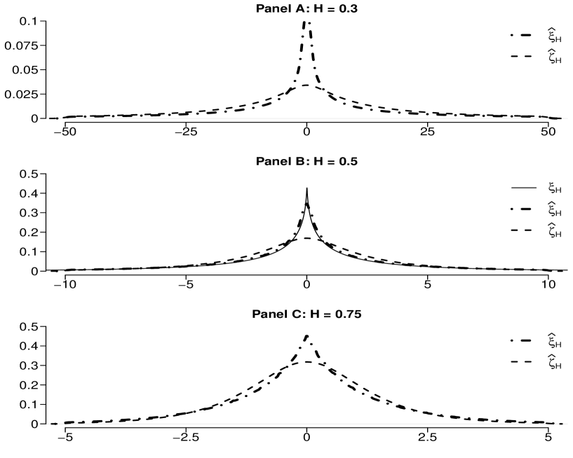
Figure 2: $\xi_{H}$: True probability function of $\xi_{H}$ for $H=0.5$. $\widehat{\xi}_{H}$: Kernel density approximation of probability density function from $\widehat{\xi}^{\;(i)}_{H}$. $\widehat{\zeta}_{H}$: Kernel density approximation of probability density function from $\widehat{\zeta}^{\;(i)}_{H}$.

5. Conclusions.

This paper presents some extensions of the results from [2] where an estimation of a singularity point of a cusp-type signal in the ”signal plus white noise” was discussed. We demonstrated that when the intensity of white noise $\varepsilon\rightarrow 0$ the limits of BE $\tilde{\theta}_{\varepsilon}^{.}$ and MLE $\hat{\theta}_{\varepsilon}$ are expressed in terms of fBm $W^{H}$ for the full range of cusp-type signals with $\alpha\in(-\frac{1}{2},\frac{1}{2})~{}$and correspondingly with the Hurst parameter $H=\alpha+\frac{1}{2}\in(0,1).~{}$The simulations results suggest that as $\varepsilon\rightarrow 0~{}$the   limit of $Var(\hat{\theta}_{\varepsilon})/Var(\tilde{\theta}_{\varepsilon}^{.})$  is a decreasing function in the range $H\in[0.3,1]~{}$showing about $40\%$ gain $\tilde{\theta}_{\varepsilon}$ over $\hat{\theta}_{\varepsilon}~{}~{}$ for $H=0.3.$ and confirming the known result for $H=\frac{1}{2}~{}$where the corresponding gain is about $35\%.~{}$

6. Acknowledgements. This paper was completed during the research stay of the third author at Tokyo Metropolitan University (TMU). We thank our colleagues from TMU for research assistance.

The authors also thank participants of Hokkaido Winter School on Finance and Mathematics (February 2017) for discussions which helped to improve the exposition of the paper.

The simulation results were obtained using the NCI National Facility in Canberra, Australia, which is supported by the Australian Commonwealth Government and on the eResearch HPCC at the University of Technology Sydney. We gratefully acknowledge Dr. Timothy Gregory Ling for kindly providing us with the C++ code for simulation of fBm, and estimation of $\zeta_{H}$ and $\xi_{H}$.

References

• [1] Borovkov, K., Mishura, Y., Novikov, A. and Zhitlukhin, M. (2017) Bounds for expected maxima of Gaussian processes and their discrete approximations. Stochastics, v. 89, no. 1, 21–37.
• [2] Chernoyarov O., Dachian, S. and Kutoyants, Yu. (2016) On parameter estimation for cusp-type signals. Annals of the Institute of Statistical Mathematics. Β Online: 07 October 2016. doi:10.1007/s10463-016-0581-x
• [3] Daniels, H. E. (1961) The asymptotic efficiency of a maximum likelihood estimator. Proc. 4th Berkeley Sympos. Math. Statist. and Prob., Univ. California Press, Berkeley, Calif., vol. I, 151–163.
• [4] Dachian, S. (2003) Estimation of cusp location by Poisson observations. Statist. Inference for Stoch. Processes. 6, 1, 1–14.
• [5] Dachian, S., Kutoyants, Yu.A. (2003) On cusp estimation of ergodic diffusion process. J. Stat. Plann. Infer. 117, 153–166.
• [6] DΓΆring, M. (2015) Asymmetric cusp estimation in regression models. Statistics: A Journal of Theoretical and Applied Stat., v.49, N.6, 1279–1297.
• [7] Gikhman, I. and Skorokhod, A. (1974) The Theory of Stochastic Processes. I. Translated from the Russian by S. Kotz. Classics in Mathematics. Springer-Verlag, Berlin.
• [8] Fujii, T. (2010) An extension of cusp estimation problem in ergodic diffusion processes. Statist. Probab. Lett., v.80, N. 9-10, 779-783.
• [9] Gushchin A., KΓΌchler U. (2011) On estimation of delay location, Stat. Inference Stoch. Process., v.14:3 , 273–305.
• [10] Ibragimov, I. and Khasminskii, R. Β (1981) Statistical Estimation. Asymptotic Theory. Springer-Verlag, New York-Berlin.
• [11] Ibragimov, I. and Khasminskii, R. (1974) The asymptotical behavior of location parameter statistical estimators for samples with continuous density with singularities”, Problems of the theory of probability distributions. Part II, Zap. Nauchn. Sem. LOMI, 41, ”Nauka”, 67–93 (In Russian).
• [12] Kim J., Pollard D. (1990) Cube root asymptotics. Ann. Stat., v.18, 191-219.
• [13] Kolmogorov, A. N. (1940). Wienersche Spiralen undeinige andere interessante Kurven im Hilbertschen Raum. C. R. (Doklady) Acad. Sci. URSS (N.S.), v.26, 115–118.
• [14] Kutoyants Yu. A. ( 1998) Statistical Inference for Spatial Poisson Processes, Lect. Notes Statist. v.134, Springer, New York.
• [15] Kutoyants, Y. (2004) Statistical Inference for Ergodic Diffusion Processes. Springer Series in Statistics. Springer-Verlag London, Ltd., London.
• [16] Mandelbrot, B. and Van Ness, J.W. (1968) Fractional Brownian motions, fractional noises and applications. SIAM Rev. v.10, 422–437.
• [17] Muravlev, A. (2011) Representation of fractal Brownian motion in terms of an infinite-dimensional Ornstein-Uhlenbeck process; translated from Uspekhi Mat. Nauk 66 (2011), no. 2(398), 235–236 Russian Math. Surveys 66, no. 2, 439–441.
• [18] Novikov, A. and Kordzakhia, N. (2013) Pitman estimators: an asymptotic variance revisited, SIAM Theory Probability and its Applications, v.57, N 3, 521-529.
• [19] Novikov, A., Kordzakhia, N. and Ling, T. (2014) On moments of Pitman estimators: the case of fractional Brownian motion, SIAM Theory Probability and its Applications, v.58, N. 4, 601-614.
• [20] Pflug, G. (1982) Statistically important Gaussian process. Stochastic Process. Appl. 13, no. 1, 45–57.
• [21] Norros, I.; Valkeila, E.; Virtamo, J. (1999) An elementary approach to a Girsanov formula and other analytical results on fractional Brownian motions. Bernoulli, v.5, no. 4, 571–587.
• [22] Pitman, E.J.G. (1939)The estimation of the location and scale parameters of a continuous population of any given form. Biometrika, v.30, 391-421
• [23] Prakasa Rao, B. L. S. (1968) Estimation of the location of the cusp of a continuous density. Ann. Math. Statist. v.39, 76–87.
• [24] Rubin, H. and Song, K. (1995) Exact computation of the asymptotic efficiency of maximum likelihood estimators of a discontinuous signal in a Gaussian white noise. Ann. Statist. v.23, no. 3, 732–739.
• [25] Samorodnitsky, G. and Taqqu, M.S. (1994) Stable Non-Gaussian Random Processes: Stochastic Models with Infinite Variance. , Chapman & Hall, Florida, USA.
• [26] Shepp, L. A. (1979) The joint density of the maximum and its location for a Wiener process with drift. J. Appl. Probab. v.16, no. 2, 423–427.
• [27] Terent’ev, A.S. (1968) Probability ditsribution of a time location of an absolute maximum at the output of a sinchronized filter. Radioengineering and Electronics, v.13, N 4, 652-657.
• [28] Wood, A. and Chan, G. (1994) Simulation of stationary Gaussian processes in [0, 1]d. Journal of Computational and Graphical Statistics, v.3, no. 4, 409–432 .
• [29] Yao, Yi-Ching (1987) Approximating the distribution of the maximum likelihood estimate of the change-point in a sequence of independent random variables. Ann. Statist. v,15, no. 3, 1321–1328.