From collective oscillation to chimera state in a nonlocally excitable system

Abstract

Chimera states, which consist of coexisting domains of spatially coherent and incoherent dynamics, have been widely found in nonlocally coupled oscillatory systems. We demonstrate for the first time that chimera states can emerge from excitable systems under nonlocal coupling in which isolated units only allow for the equilibrium. We theoretically reveal that nonlocal coupling induced collective oscillation is behind the occurrence of the chimera states. We find two different types of chimera states, phase-chimera state and excitability-chimera states, depending on the coupling strength. At weak coupling strength where collective oscillation is localized around the unstable homogeneous equilibrium, the chimera states are similar to the ones in nonlocally coupled phase oscillators. For the chimera states at strong coupling strength, the dynamics of both coherent units and incoherent units shift back and forth between low amplitude oscillation induced by collective oscillation and high amplitude oscillation induced by excitability of local units.

Keywords: chimera states, excitable system, collective motion

1 Introduction

Chimera states refer to a type of fascinating hybrid dynamical states in which identically coupled units spontaneously develop into coexisting synchronous and asynchronous parts. The chimera states were first found numerically by Kuramoto and his colleagues in 2002 [1], theoretically investigated by Strogatz and his colleagues in 2004 [2], and then have become a very active research field [3, 4, 5]. The chimera states were realized experimentally in chemical [6, 7], optical [8, 9], electronical [10], mechanical and electrochemical systems [11, 12, 13, 14]. Chimera states are also possibly related to Parkinson’s diseases where synchronized activities are absent in certain regions of the brain [15], and epileptic seizures where specific regions of the brain are highly synchronized while other parts are not synchronized [16, 17]. Different types of chimera states such as breathing chimeras [2], amplitude-mediated chimeras [18], multi-cluster chimeras [19, 20, 21], and spiral chimeras [22, 23] have been discovered and investigated in details.

Chimera states are initially observed in nonlocally coupled phase oscillators, and both nonlocal coupling and phase oscillators are thought to be required for realizing chimera states. But it has been extensively observed that chimera states can occur in globally coupled [24, 25] and locally coupled oscillators [26], periodic and chaotic maps [27], Stuart-Landau models [28, 18], Van der Pol oscillators [29], FitzHugh-Nagumo (FHN) oscillators [30], Hindmarsh-Rose models [31], Hodgkin-Huxley models [32] and delayed-feedback systems [10]. However, these systems still have one common requirement that each individual unit is self-oscillating when it is isolated. Then one great and interesting question arises: if isolated unites do not support self-oscillation, can chimera states be realized when they are nonlocally coupled?

Excitable systems with a stable equilibrium are ubiquitous in biology, chemistry, and physics [33, 34]. In an excitable system, it takes a large excursion before going back to the equilibrium if perturbations are stronger than a threshold. Recently, chimera states have been studied in nonlocally coupled type-I excitable systems [35] and nonlocally coupled excitable systems in the presence of noise [36]. But the isolated units in these works are still self-oscillating rather than the follow a stable equilibrium. In this paper, we will demonstrate that chimera states can be realized in a nonlocally coupled excitable system in which each isolated unit only allows for an equilibrium rather than a self-oscillation.

The rest of paper is organized as follows. In section 2, we present the model and numerical demonstrate the existence of chimera dynamics. In section 3, we present the stability analysis on the homogeneous equilibrium and demonstrate the emergence of collective oscillation, followed by the numerical results on the transition scenario from homogeneous equilibrium to chimera dynamics. In section 4, we address the roles of model parameters on chimera dynamics. Finally, we conclude with a summary in section 5.

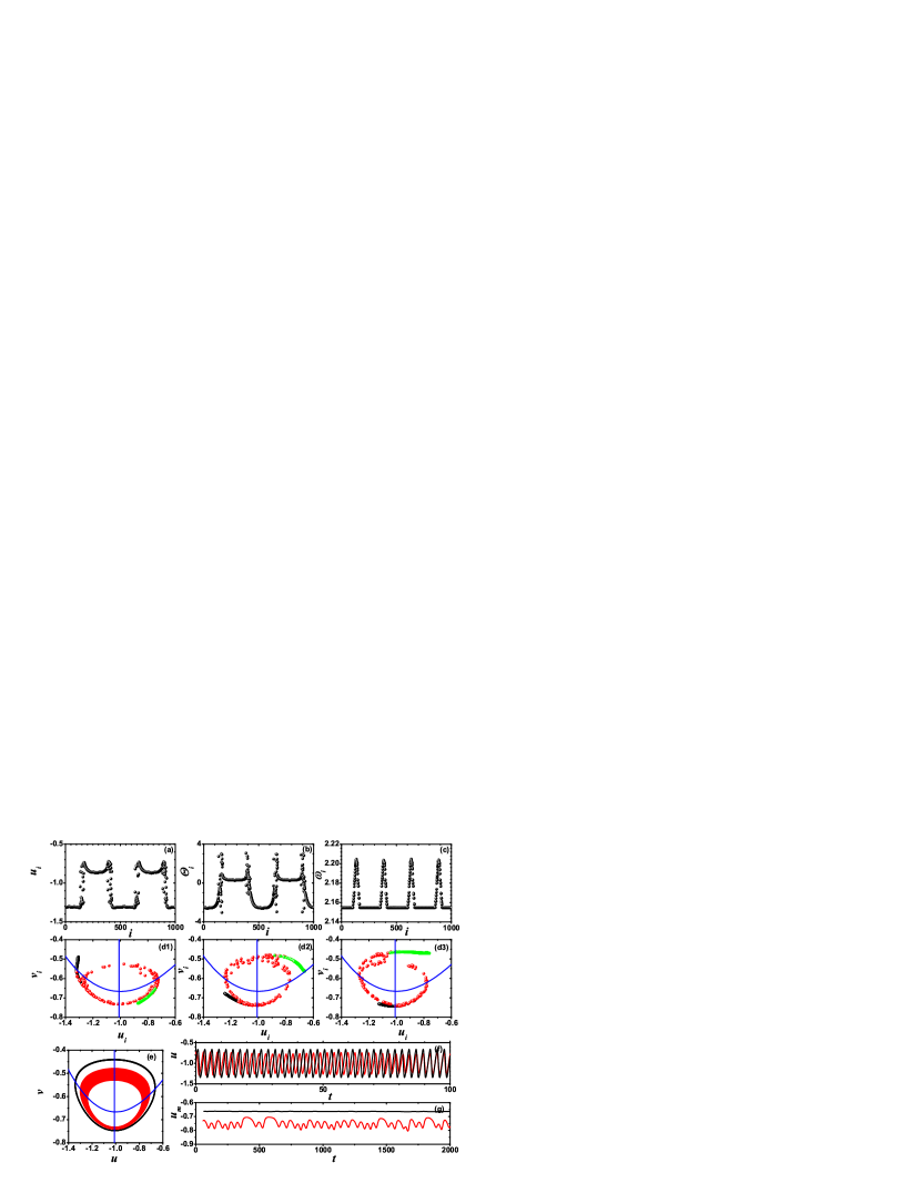
Figure 1: (color online)(a) Snapshot of the variables $u_{i}$. (b) Snapshot of the phases $\Theta_{i}$. (c) Mean phase velocities $\omega_{i}$. (d1)-(d3) Snapshots in the ($u_{i},v_{i}$) plane at different times (blue lines denote the nullclines of the FHN unit). Incoherent units denoted by red dots, the units in adjacent clusters denoted by black and green dots, respectively. (e) The trajectories of one coherent (in black) and one incoherent (in red) FHN units. (f) The time sequence of the coherent (in balck) and the incoherent (in red) units. (g) The evolution of the maximum of $u$, $u_{m}$ for the coherent (black) and the incoherent I in red) units. $\phi=\pi/2+0.57$, $\sigma=0.05$. In the numerical simulations, we employ a fourth-order Runge-Kutta algorithm with a time step $\delta t=0.01$. Random initial conditions are used.

2 The model

We consider a one-dimensional ring of $N$ nonlocally coupled FHN systems [30] in which the individual unit is coupled to $R$ neighbors on each side with coupling strength $\sigma$:

$$\epsilon\dot{u}_{i} = u_{i}-\frac{u_{i}^{3}}{3}-v_{i}$$

$$+ \frac{\sigma}{2R}\Sigma_{j=i-R}^{i+R}[b_{uu}(u_{j}-u_{i})+b_{uv}(v_{j}-v_{i})],$$

$$\dot{v}_{i} = u_{i}+a$$ (1)

$$+ \frac{\sigma}{2R}\Sigma_{j=i-R}^{i+R}[b_{vu}(u_{j}-u_{i})+b_{vv}(v_{j}-v_{i})].$$

The subscript $i$ refers to the unit index, which has to be taken module $N$ (or period boundary condition). $u_{i}$ and $v_{i}$ are the activator and inhibitor variables, respectively. $\epsilon>0$ is the parameter characterizing a time separation. Following the reference [30], the coupling matrix is modelled as:

$$B=\left(\begin{array}[]{cc}b_{uu}&b_{uv}\\ b_{vu}&b_{vv}\\ \end{array}\right)=\left(\begin{array}[]{cc}\cos\phi&\sin\phi\\ -\sin\phi&\cos\phi\\ \end{array}\right).$$ (6)

It is convenient to consider the ratio $r=R/N$, the coupling radius, which ranges from $1/N$ (nearest neighbor coupling) to $0.5$ (globally coupling). Isolated FHN unit exhibits excitable behavior for $|a|>1$ while oscillatory behavior for $|a|<1$ via a Hopf bifurcation at $|a|=1$. Because our study focuses on the excitable regime, we set $a=1.01$, $\epsilon=0.18$, $r=0.35$ and $N=1000$ throughout the letter. So the isolated units of Eq.(2) have an equilibrium $(u^{*},v^{*})=(-a,-a+a^{3}/3)$.

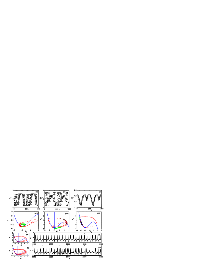
Figure 2: (color online)(a) Snapshot of the variables $u_{i}$. (b) Snapshot of the phases $\Theta_{i}$. (c) Mean phase velocities $\omega_{i}$. (d1)-(d3) Snapshots in the ($u_{i},v_{i}$) plane at different times (blue lines denote the nullclines of the FHN unit). Incoherent units denoted by red dots, the units in adjacent clusters denoted by black and green dots, respectively. (e) and (f) The trajectories of one coherent and one incoherent FHN units, respectively. (g) and (h) The time sequence of the coherent and the incoherent units, respectively. $\phi=\pi/2+0.57$, $\sigma=0.18$.

By increasing the coupling strength $\sigma$, we find that chimera states do exist for nonlocally coupled excitable FHN units. Specially, two types of chimera states are discovered. For chimera states at weak coupling strength, FHN units oscillate near the equilibrium $(u^{*},v^{*})$. On the other hand, chimera states at strong coupling strength display strong characteristics of the excitability.

The chimera state at weak coupling strength $\sigma=0.05$ is shown in Fig. 1. The snapshot of the activator variables $u_{i}$ in Fig. 1(a) suggests a chimera state with four same size coherent clusters, separated by four same size narrow incoherent clusters. The snapshot of the phases of FHN units, defined as $\Theta_{i}=\arctan(\dot{v}_{i}/\dot{u}_{i})$, in Fig. 1(b) shows that adjacent coherent clusters are in antiphase, which is same as those clustered chimera states observed in nonlocally coupled phase oscillators [37, 21]. (To be noted, in the case of coexisting large- and small-amplitude oscillations in Fig. 2, the definition of the phase $\Theta_{i}$ by $\dot{v}_{i}$ and $\dot{u}_{i}$ is much more convenient than the one by $v_{i}$ and $u_{i}$ in calculating the mean phase velocities of FHN units). The coherent and incoherent clusters can be distinguished from each other through the mean phase velocity of each FHN unit, defined as $\omega_{i}=\langle\dot{\Theta}_{i}\rangle_{t}$ with $\langle\cdot\rangle_{t}$ the time average over a long time interval. The profile of $\omega_{i}$ in Fig. 1(c) shows that FHN units in the coherent clusters have the same mean phase velocity, denoted as $\Omega$, while those in the incoherent clusters have different $\omega_{i}$ which are always larger than $\Omega$. The snapshots of FHN units in the $(u_{i},v_{i})$ plane at different specific times in Fig. 1(d1)-(d3) show that the units in coherent clusters are concentrated on two pieces of curves opposite to the equilibrium and units from adjacent coherent clusters fall into different curves. In contrast, FHN units in incoherent clusters are scattered on noisy orbits between these two curves.

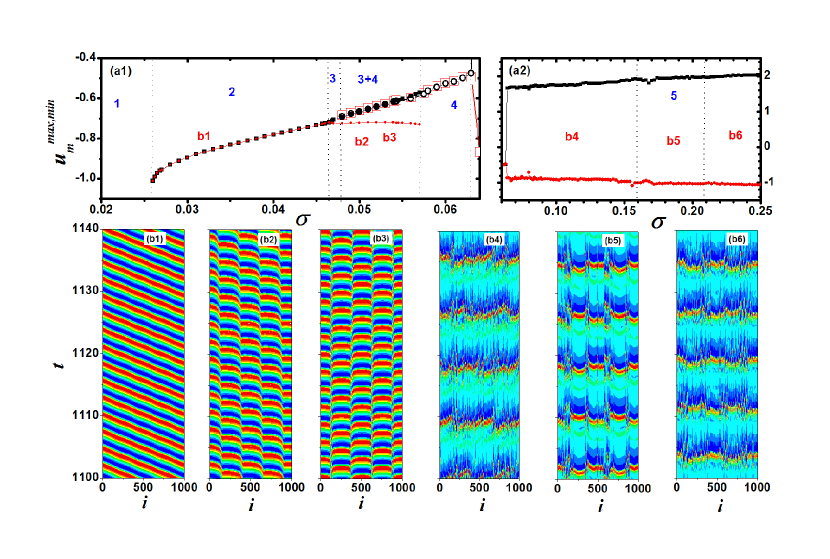
Figure 3: (color online)(a1) and (a2) $u_{m}^{max}$ (in black) and $u_{m}^{min}$ (in red) are plotted against $\sigma$. Solid symbols are obtained from the forward continuation and open symbols from the backward continuation. The numbers denote different dynamical regimes (see main text). In the regime denoted by $"3+4"$, the modulated travelling wave states and the phase-chimera states coexist. (b1)-(b6) The spatial-temporal plots of $u_{i}$ at the coupling strengthes denoted by b1-b6 in (a).

The FHN units in coherent and incoherent clusters obey different dynamics. Figure 1(e) shows the trajectories of two typical FHN units, the limit cycle for the coherent unit and the torus-like trajectory for the incoherent unit. The torus-like trajectory is enclosed by the limit cycle and both trajectories are localized around the equilibrium $(u^{*},v^{*})$. $u(t)$ of the two units in Fig. 1(f) show that the incoherent unit oscillates faster than the coherent one and its amplitude varies with time. Furthermore, the evolutions of the maximum of $u(t)$, $u_{m}(t)$, for the two units in Figs. 1(g) and (h) show a periodic oscillation for the coherent unit while irregular dynamics for the incoherent unit.

As the coupling strength $\sigma$ is increased into a strong couple strength region, an different and interesting type of chimera state is emerged and presented in Fig. 2 at coupling strength $\sigma=0.18$. In comparison with the one in Fig. 1, there are two remarkable differences. Firstly, the profile of $\omega_{i}$ in Fig. 2(c) indicates that coherent FHN units oscillate faster than incoherent FHN units. Secondly, the snapshots of FHN units in the $(u_{i},v_{i})$ plane in Fig. 2(d1)-(d3) remarkably show that the oscillation of FHN units is not localized near $(u^{*},v^{*})$. Instead, FHN units shift back and forth between the low amplitude oscillation around the equilibrium and the high amplitude oscillation with the excursion characteristics of excitable dynamics. It can be further evidenced by the trajectories of one coherent unit in Fig. 2(e) and one incoherent unit in Fig. 2(f). The time sequence of $u$ in Fig. 2(g) shows that the coherent unit alternates between two intertwined temporal patterns, one cycle of small amplitude oscillation followed by one cycle of high amplitude oscillation, and two cycles of small amplitude oscillation followed by one cycle of high amplitude oscillation. In contrast, the incoherent unit displays irregular behaviors between the low and the high amplitude oscillations in Fig. 2(h). In addition, the $\pi$ phase difference between the adjacent coherent clusters is not held any more, which is clearly shown in Fig. 2(b).

3 The emergence of collective oscillation and the transition to chimera dynamics

How can FHN units support chimera states when they are in excitable regime? In other words, where does the oscillation for each unit emerge from? Our work reveals that a collective motion can be induced through the nonlocal coupling. If the coupling strength is higher than a critical value, the homogeneous equilibrium $(u^{*},v^{*})$ becomes unstable and a collective motion in the form of travelling wave emerges. To elucidate it, we analyze the stability of the homogeneous equilibrium $(u^{*},v^{*})$ in details. The evolution of the perturbation $(\delta u_{i},\delta v_{i})$ near $(u^{*},v^{*})$ follows

$$\frac{d}{dt}(\begin{array}[]{c}\delta u_{i}\\ \delta v_{i}\end{array})=DF(u^{*},v^{*})(\begin{array}[]{c}\delta u_{i}\\ \delta v_{i}\end{array})+\Sigma_{j=i-R}^{i+R}\bar{B}(\begin{array}[]{c}\delta u_{j}-\delta u_{i}\\ \delta v_{j}-\delta v_{i}\end{array})$$ (13)

with $DF(u^{*},v^{*})=\left(\begin{array}[]{cc}(1-u^{*2})/\epsilon&-1/\epsilon\\ 1&0\\ \end{array}\right)$ and $\bar{B}=\left(\begin{array}[]{cc}b_{uu}/\epsilon&b_{uv}/\epsilon\\ b_{vu}&b_{vv}\\ \end{array}\right)$. For the model (1), there are $N$ spatial modes characterized by the vectors $\nu_{k}=(1,\omega_{k},\omega_{k},...,\omega_{k}^{N-1})^{T}/\sqrt{N}$, ($k=1,2,...,N-1$) where $\omega_{k}=\exp(\mathbf{i}2\pi k/N)$ with $\mathbf{i}$ the imaginary unit and $k$ the wave number. Expanding the perturbation over these spatial modes and substituting it into the Eq. (13), we have

$$\dot{\delta}_{k}=(DF(u^{*},v^{*})+\sigma\lambda_{k}\bar{B})\delta_{k}=DF^{(k)}(u^{*},v^{*})\delta_{k}$$ (14)

with

$$\lambda_{k} = -1+\frac{\cos\frac{2\pi kR}{N}-\cos\frac{2\pi k(R+1)}{N}+\cos\frac{2\pi k}{N}-1}{2R(1-\cos\frac{2\pi k}{N})}$$ (15)

Either the determinant $Det(DF^{(k)})<0$ or the trace $Tr(DF^{(k)})>0$ when $Det(DF^{(k)})>0$ leads the spatial mode $\nu_{k}$ to be unstable. The latter leads $\delta_{k}$ to grow in an oscillating way and the former leads $\delta_{k}$ to grow monotonically in an exponential way. It can be shown that $Det(DF^{(k)})>0$ is always satisfied for the parameters used in this letter. Therefore, once $Tr(DF^{(k)})>0$, the spatial mode $\nu_{k}$ becomes unstable through a Hopf bifurcation. For each spatial mode, we have its critical coupling strength $\sigma^{(k)}_{c}=(a^{2}-1)/(1+\epsilon)\lambda_{k}\cos\phi$. Since $\lambda_{k}$ is always negative, $\cos\phi<0$ is required to have a positive $\sigma^{(k)}_{c}$. Clearly, the most unstable spatial mode $\nu_{k^{*}}$ has the largest $|\lambda_{k}^{*}|$. When $\sigma>\sigma^{(k^{*})}_{c}$, the homogeneous equilibrium becomes unstable and a travelling wave with the wave number $k^{*}$ appears and renders the oscillation to each FHN unit. For the parameters in Figs. 1 and 2, we obtain $k^{*}=2$ and $\sigma^{(k^{*})}_{c}=0.026$. The low amplitude oscillation there roots in the collective oscillation while the high amplitude oscillation results from the limit cycle induced by the excitability of local units. In this respect, we call the chimera states in Fig. 1 the phase-chimera states and the ones in Fig. 2 the excitability-chimera states.

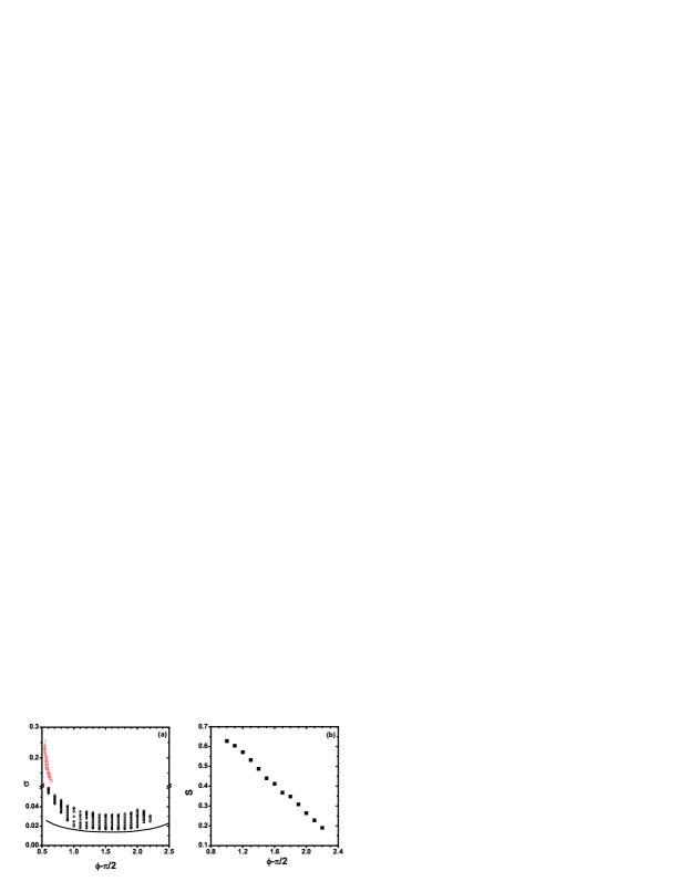
Figure 4: (color online)(a) The stability regimes for phase-chimera states (black dots) and excitability-chimera states (red plus) in the plane of $\sigma$ and $\phi$. The black curve denotes the onset of the collective motion below which the homogeneous equilibrium is stable. (b) The dependence of the fraction of coherent units, $S$, on $\phi$, at $\sigma=0.03$.

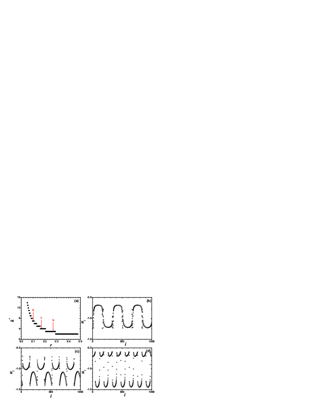
Figure 5: (color online)(a) The wave number $k^{*}$ of the most unstable spatial mode to the homogeneous equilibrium $(u^{*},v^{*})$ is plotted against $r$. Red alphabets b, c, and d denote parameter values for plots (b) , (c), and (d). The snapshots of the variables $u_{i}$ at $r=0.27$ and $\sigma=0.05$ in (b), at $r=0.17$ and $\sigma=0.06$ in (c), at $r=0.1$, and $\sigma=0.06$ in (d).

To study the transition scenario from the travelling waves to the chimera states, we consider two types of bifurcation diagrams, forward continuation and backward continuation. The coupling strength $\sigma$ is successively increased (or decreased) by a $\delta\sigma$ in the forward (or backward) continuation and the initial conditions for one coupling strength are the final state of the previous one. We monitor the evolution of $u_{m}$ for a coherent FHN unit (or for an arbitrary FHN unit if there is no coherent one). The maximum and the minimum of $u_{m}$, $u_{m}^{max}$ and $u_{m}^{min}$, are measured and their dependence on $\sigma$ are presented in Fig. 3(a1) and (a2). There are several dynamical regimes. The homogeneous equilibrium $(u^{*},v^{*})$ is stable for $\sigma<0.026$ (the regime 1). In the regime 2 where $u_{m}^{max}=u_{m}^{min}$, the coherent unit oscillates periodically and its oscillation amplitude $u_{m}^{max}-u^{*}$ increases with $\sigma$. As shown by the spatial-temporal plot of $u$ in Fig. 3(b1), travelling wave states are realized in this regime. Increasing $\sigma$ from the regime 2, the travelling wave state becomes unstable at $\sigma\approx 0.046$ and a modulated travelling wave (see Fig. 3(b2)) occurs in the regime 3. $u_{m}^{max}\neq u_{m}^{min}$ in the regime 3, which suggests the quasiperiodic motion for FHN units. At stronger coupling strength $\sigma$, $u_{m}^{max}$ becomes equal to $u_{m}^{min}$ again as shown in the regime 4 in which the phase-chimera state is realized (see Fig. 3(b3)). By comparing the results from the forward and backward continuations, we find that the phase-chimera states coexist with the modulated travelling waves in the range $0.048<\sigma<0.057$. The phase-chimera state becomes unstable around $\sigma=0.063$ at which the oscillation amplitudes of FHN units become strong enough to trigger the excitability of FHN units. Consequently, the oscillations of FHN units are not localized near their equilibria as $\sigma$ is beyond $0.063$. They always shift back and forth between the small amplitude and high amplitude oscillations characterized by $u_{m}^{min}$ and $u_{m}^{max}$ respectively. Together with Figs. 3(a2), the spatial-temporal plots of $u$ in Figs. 3(b4) -(b6) indicate that excitability-chimera state only exists in the regime 5 and there is no clear difference between the dynamics in the regimes 4 and 6.

4 The impact of the model parameters on chimera dynamics

To further investigate the chimera dynamics, we present in Fig. 4(a) the phase diagram in the plane of $\sigma$ and $\phi$ in which the regime with red pluses supports the excitability-chimera is denot while the regime with black circles supports the phase-chimera. As shown in Fig. 4(a), the excitability-chimera states exist within a narrow range of $\phi$ at strong coupling strength. On the other hand, the phase-chimera states can exist in the parameter regime with $\phi$ spanning from 2.1 to 3.8 but a narrow range of $\sigma$. The parameter $\phi$ has strong impacts on the fraction of the coherent units in the population, defined as $S=N_{c}/N$ with $N_{c}$ the number of coherent units, for the phase-chimera state. Figure 4(b) clearly shows a linear dependence of $S$ on $\phi$. We also numerically find that the total number of coherent clusters in the phase-chimera state is twice of the wave number $k^{*}$, which is mainly determined by the coupling radius $r$. The relation of $k^{*}$ against $r$ is shown in Fig. 5(a). It clearly shows that $k^{*}$ tends to 2 even when $r$ approaches 0.5. This suggests nonexistence of the phase-chimera state with 1 or 2 coherent clusters in the nonlocally coupled FHN system (1). The snapshots of the variable $u_{i}$ at three different $r$ are shown in Fig. 5(b)-(d), respectively. The corresponding number of coherent clusters is 6, 8 and 14, which is exact twice of the wave number $k^{*}$.

5 Conclusions

In previous investigations on chimera dynamics, the isolated unit has to be oscillatory, either self-oscillation or noise-induced-oscillation due to the coherent resonance. In this paper, we reported the existence of chimera states in a nonlocally coupled FHN system in the excitable regime where isolated unit only allows for the solution of equilibrium. The findings in this paper suggest that the emergence of chimera states is not restricted to oscillatory systems. We find that the collective oscillation induced by nonlocal coupling plays critical roles for the emergence of chimera states in this system. For sufficiently weak coupling strength, the nonlocally coupled systems only support homogeneous equilibrium. However, when the coupling strength is beyond a critical value, the homogeneous equilibrium becomes unstable and a travelling wave state is born, which makes units to oscillate and makes the appearance of chimera states to be possible. Depending on the coupling strength, two types of chimera states are observed. The first type of chimera state occurs at weak coupling strength in which both coherent and incoherent FHN units oscillate with low amplitude around the equilibrium of isolated unit. The second type of chimera state appears in the strong coupling strength, in which the dynamics of both coherent and incoherent units shifts back and forth between the low amplitude oscillation around their equilibria and the high amplitude oscillation following the excited limit cycle. We also numerically find that the total number of coherent clusters in these chimera states is determined by the coupling radius and is twice of the wave number of the travelling wave born out of the homogeneous equilibrium. Although our revealed findings are based on the FHN systems, the emergence of chimera states by nonlocal coupling induced collective oscillation should not depend on the specific system, and can be realized in other excitable systems.

References

References

- [1] Kuramoto Y and Battogtkh D 2002 Coexistence of coherence and incoherence in nonlocally coupled phase oscillators Nonlinear Phenom. Complex Syst. 5 380-5
- [2] Abrams D M and Strogatz S H 2004 Chimera states for coupled oscillators Phys. Rev. Lett. 93 174102
- [3] Panaggio M J and Abrams D M 2015 Chimera states: coexistence of coherence and incoherence in networks of coupled oscillators Nonlinearity 28 R67-87
- [4] Abrams D M, Mirollo R, Strogatz S H and Wiley D A 2008 Solvable model for chimera states of coupled oscillators Phys. Rev. Lett. 101 084103
- [5] Pikovsky A and Rosenblum M 2008 Partially integrable dynamics of hierarchical populations of coupled oscillators Phys. Rev. Lett. 101 264103
- [6] Tinsley M R, Nkomo S and Showalter K 2012 Chimera and phase-cluster states in populations of coupled chemical oscillators Nat. Phys. 8 662-5
- [7] Schmidt L, Schönleber K, Krischer K and García-Morales V 2014 Coexistence of synchrony and incoherence in oscillatory media under nonlinear global coupling Chaos 24 013102
- [8] Hagerstrom A M, Murphy T E, Roy R, Hövel P, Omelchenko I and Schöll E 2012 Experimental observation of chimeras in coupled-map lattices Nat. Phys. 8 658-61
- [9] Viktorov E A, Habruseva T, Hegarty S P, Huyet G and Kelleher B 2014 Coherence and incoherence in an optical comb Phys. Rev. Lett. 112 224101
- [10] Larger L, Penkovsky B and Maistrenko Y 2013 Virtual chimera states for delayed-feedback systems Phys. Rev. Lett. 111 054103.
- [11] Martens E A, Thutupalli S, Fourrière A and Hallatschek O 2013 Chimera states in mechanical oscillator networks. Proc. Natl. Acad. Sci. 110 10563-7
- [12] Kapitaniak T, Kuzma P, Wojewoda J, Czolczynski K and Maistrenko Y 2014 Imperfect chimera states for coupled pendula Sci. Rep. 4 6379
- [13] Olmi S, Martens E A, Thutupalli S and Torcini A 2015 Intermittent chaotic chimeras for coupled rotators Phys. Rev. E 92 030901(R)
- [14] Wickramasinghe M and Kiss I Z 2013 Spatially organized dynamical states in chemical oscillator networks: synchronization, dynamical differentiation, and chimera patterns PLoS ONE 8 e80586
- [15] Levy R, Hutchison W D, Lozano A M and Dostrovsky J O 2000 High-frequency synchronization of neuronal activity in the subthalamic nucleus of parkinsonian patients with limb tremor J. Neurosci. 20 7766-75
- [16] Motter A E 2010 Nonlinear dynamics: Spontaneous synchrony breaking Nat. Phys. 6 164-5
- [17] Ayala G F, Dichter M, Gumnit R J, Matsumoto H and Spencer W A 1973 Genesis of epileptic interictal spikes. New knowledge of cortical feedback systems suggests a neurophysiological explanation of brief paroxysms Brain Res. 52 1-17
- [18] Zakharova A, Kapeller M and Schöll E 2014 Chimera death: Symmetry breaking in dynamical networks Phys. Rev. Lett. 112 154101
- [19] Omelchenko I, Provata A, Hizanidis J, Schöll E and Hövel P 2015 Robustness of chimera states for coupled FitzHugh-Nagumo oscillators Phys. Rev. E 91 022917
- [20] Maistrenko Y L, Vasylenko A, Sudakov O, Levchenko R and Maistrenko V L 2014 Cascades of multiheaded chimera states for coupled phase oscillators Int. J. Bifurcat. Chaos 24 1440014
- [21] Zhu Y, Li Y, Zhang M and Yang J 2012 The oscillating two-cluster chimera state in non-locally coupled phase oscillators EPL 97 10009
- [22] Martens E A, Laing C R and Strogatz S H 2010 Solvable model of spiral wave chimeras Phys. Rev. Lett. 104 044101
- [23] Gu C, St-Yves G and Davidsen J 2013 Spiral wave chimeras in complex oscillatory and chaotic systems Phys. Rev. Lett. 111 134101
- [24] Sethia G C and Sen A 2014 Chimera states: The existence criteria revisited Phys. Rev. Lett. 112 144101
- [25] Schmidt L and Krischer K 2015 Clustering as a Prerequisite for Chimera States in Globally Coupled Systems Phys. Rev. Lett. 114 034101
- [26] Laing C R 2015 Chimeras in networks with purely local coupling Phys. Rev. E 92 050904(R)
- [27] Omelchenko I, Maistrenko Y, Hövel P and Schöll E 2011 Loss of coherence in dynamical networks: Spatial chaos and chimera states Phys. Rev. Lett. 106 234102
- [28] Laing C R 2010 Chimeras in networks of planar oscillators Phys. Rev. E 81 066221
- [29] Omelchenko I, Zakharova A, Hövel P, Siebert J and Schöll E 2015 Nonlinearity of local dynamics promotes multi-chimeras Chaos 25 083104
- [30] Omelchenko I, Omelchenko O E, Hövel P and Schöll E 2013 When nonlocal coupling between oscillators becomes stronger: Patched synchrony or multichimera states Phys. Rev. Lett. 110 224101
- [31] Hizanidis J, Kanas V, Bezerianos A and Bountis T 2014 Chimera states in networks of nonlocally coupled Hindmarsh-Rose neuron models Int. J. Bifurcat. Chaos 24 1450030
- [32] Sakaguchi H 2006 Instability of synchronized motion in nonlocally coupled neural oscillators Phys. Rev. E 73 031907
- [33] Winfree A T 1972 Spiral waves of chemical activity Science 175 634-6
- [34] Zykov V S 1987 Simulation of Wave Processes in Excitable Media (Manchester Univ. Press, Manchester, UK)
- [35] Vülings A, Hizanidis J, Omelchenko I and Hövel P 2014 Clustered chimera states in systems of type-I excitability New. J. Phys. 16 123039
- [36] Semenova N, Zakharova A, Anishchenko V and Schöll E 2016 Coherence-resonance chimeras in a network of excitable elements Phys. Rev. Lett. 117 014102
- [37] Sethia G C, Sen A and Atay F M 2008 Clustered chimera states in delay-coupled oscillator systems Phys. Rev. Lett. 100 144102