Abstract

Generation of different nonequilibrium states in trapped Bose-Einstein condensates is studied by numerically solving nonlinear Schrödinger equation. Inducing nonequilibrium states by shaking the trap, the following states are created: weak nonequilibrium, the state of vortex germs, the state of vortex rings, the state of straight vortex lines, the state of deformed vortices, vortex turbulence, grain turbulence, and wave turbulence. A characterization of nonequilibrium states is advanced by introducing effective temperature, Fresnel number, and Mach number.

Keywords: Trapped atoms, Bose-Einstein condensate, nonequilibrium states, vortex germs, vortex rings, vortex lines, vortex turbulence, grain turbulence, wave turbulence, classification of states

PACS numbers: 03.75.Kk, 03.75.Lm, 03.75.Nt, 67.85.De, 67.85.Jk

1 Introduction

The most widely studied nonequilibrium state of quantum fluids is quantum turbulence [1, 2, 3, 4, 5]. Recently, quantum turbulence has got a lot of attention in the studies of cold atomic systems, as can be inferred form the review articles [4, 5, 6, 7]. The creation of strongly nonequilibrium atomic states of Bose-Einstein condensates by shaking a trap, as suggested in Refs. [8, 9], has made it possible to experimentally realize quantum turbulence of cold atomic gases in harmonic traps (see reviews [5, 6, 7]) and in a box-shaped trap [10].

But quantum turbulence is not the sole nonequilibrium state that can be generated by shaking a trap. Other nonequilibrium states, such as grain turbulence and wave turbulence can be generated in experiment and analyzed numerically by solving the nonlinear Schrödinger (NLS) equation [11, 12, 13, 14].

An important question is: How would it be possible to ascribe a quantitative characteristic to different nonequilibrium states that could be generated in trapped Bose-condensed systems? For classical liquids, laminar and turbulent flows are distinguished by the Reynolds number $Re=vL/\nu$, where $v$ is a characteristic flow velocity, $L$ is a characteristic linear system size, and $\nu$ is kinematic viscosity [15]. The characterization of flows by Reynolds numbers is also applicable to quantum liquids, such as superfluid helium [16]. However, for cold atomic gases, at low temperatures, viscosity is zero, so that the Reynolds number becomes infinite [17]. For describing the motion of obstacles through atomic superfluid gas, the Strouhal number $St=fL/v$ can be used [18, 19], where $f$ is the vortex shedding frequency. Various patterns of vortex shedding can arise in quantum fluids behind moving obstacles [20, 21].

However, the problem of characterizing various nonequilibrium states that could arise in trapped atomic Bose-condensed systems, without any obstacles, remains unsolved.

The aim of the present paper is twofold. First, we thoroughly analyze what qualitatively different nonequilibrium states can appear in trapped Bose-Einstein condensates when the trapping potential is perturbed by time-dependent modulation. Second, we suggest a quantitative characterization of all such states by three quantities, effective temperature, Fresnel number, and Mach number.

The use of the Fresnel number is motivated by the analogy between nonequilibrium states of atomic systems and optical phenomena in lasers, where the terms optical turbulence or photon turbulence are well known. The Mach number has also been used for characterizing turbulent flows in geophysics, as is discussed in the book by Smits and Dussauge [22]. Fresnel numbers for trapped cold atoms have also been discussed in the context of superradiant Rayleigh scattering [23]. These analogies suggest that the mentioned characteristics can be useful for describing nonequilibrium states of trapped atoms.

Our goal is to model the behavior of Bose-Einstein condensate by numerically solving the three-dimensional time-dependent nonlinear Schrödinger equation describing the system of Bose-condensed atoms [24]. The system parameters are chosen exactly coinciding with the recent experiments [25, 26] with ⁸⁷Rb. This choice allows us to compare our numerical results with the available experimental data. But such a comparison is not the aim of the present paper, since it has already been done in our previous publications [12, 13, 14] and good agreement between numerical and experimental data has been observed. In the present paper, we concentrate on a more detailed numerical investigation of arising nonequilibrium states, finding additional types of the states, such as vortex germs, vortex rings, and strongly deformed vortices that have not been observed in the earlier publications. [12, 13, 14]. The most important point of the present paper is the suggested novel characterization of nonequilibrium states. We illustrate this characterization by nonequilibrium states generated in trapped Bose-Einstein condensates. But this characterization, being formulated in general terms, can be applied to any other nonequilibrium states.

In the brief letter [13] we studied experiments with nonequilibrium trapped atoms and the interpretation of the experimentally observed states. The discussed experiments exhibit only three such states: separate vortices, vortex turbulence, and grain turbulence. While in the present paper, we accomplish a detailed numerical investigation of all possible nonequilibrium states, distinguishing eight different states: weak nonequilibrium, vortex germs, vortex rings, vortex lines, deformed vortices, vortex turbulence, grain turbulence, and wave turbulence. Also, the injected energy, considered in [13], turned out to be not the most convenient quantity, because of which we suggest here new characteristics.

Defining such dimensionless quantities as a Fresnel and Mach number is useful in that they allow for comparison between systems with different geometries and length scales and also between different physical systems. In this light, defining a Fresnel number for a BEC allows one to draw parallels between optical and atomic nonequilibrium states, e.g., such as turbulence.

The transitions between the observed nonequilibrium states are not sharp phase transitions, but they are gradual crossovers. However, each state is qualitatively different from others, because of which they can be well distinguished from each other and classified as separate states. The gradual crossover transitions are typical for finite systems and for nonequilibrium phenomena [27].

2 Generation of nonequilibrium states

We choose the same setup as has been used in the recent experiments [25, 26] with ⁸⁷Rb. At the initial moment of time, all atoms of ⁸⁷Rb, with the mass $m=1.445\times 10^{-22}$g and the scattering length $a_{s}=0.577\times 10^{-6}$ cm, are assumed to be Bose-condensed in a cylindrical harmonic trap with the radial frequency $\omega_{r}=2\pi\times 210$ Hz and the axial frequency $\omega_{z}=2\pi\times 23$ Hz. The total number of atoms $N=1.5\times 10^{5}$. The atomic cloud has the radius $R_{eff}=4\times 10^{-4}$ cm and length $L_{eff}=6\times 10^{-3}$ cm. The central density is $\rho=2.821\times 10^{14}$ cm^-3. The healing length is $\xi=1.106\times 10^{-5}$ cm.

As usual, for numerical calculations, it is convenient to write the time-dependent equation in a dimensionless form, with the energies measured in units of the characteristic oscillator frequency $\omega_{0}\equiv(\omega_{r}^{2}\omega_{z})^{1/3}$, time measured in units of $\omega_{0}^{-1}$, and lengths measured in units of the characteristic oscillator length $l_{0}\equiv\sqrt{\hbar/m\omega_{0}}$. Here $\omega_{0}=630$ s^-1 and $l_{0}=1.08\times 10^{-4}$ cm.

Starting from the initial time, the trap is subject to the action of a perturbing alternating potential, such that the trapping potential, in dimensionless units, takes the form

$$V({\bf r},t)=\frac{1}{2}\left\{\frac{1}{\alpha^{2}}\;[x\cos\vartheta_{1}+y\sin\vartheta_{1}-z\sin\vartheta_{2}-\delta_{1}(1-\cos\omega t)]^{2}\right.+$$

$$+\left.[y\cos\vartheta_{1}-x\sin\vartheta_{1}-\delta_{2}(1-\cos\omega t)]^{2}+[z\cos\vartheta_{2}+x\sin\vartheta_{2}-\delta_{3}(1-\cos\omega t)]^{2}\right\}\;.$$ (1)

Here $\alpha\equiv\omega_{z}/\omega_{r}$ is aspect ratio, $\vartheta_{i}=A_{i}(1-\cos\omega t)$, $A_{1}=\pi/60$, $A_{2}=\pi/120$, $\delta_{1}=1.861A$, $\delta_{2}=4.653A$, $\delta_{3}=2.792A$, the effective modulation amplitude $A=0.2$, and the modulation frequency is $\omega=2\pi\times 200$ Hz. These parameters could be varied, which, as we have checked, does not qualitatively change the overall picture. So, in numerical calculations, we keep them as defined above. The alternating trapping potential shakes the atomic cloud without imposing a moment of rotation.

Dynamics of the trapped Bose condensate is analyzed by numerically solving the nonlinear Schrödinger (NLS) equation defined on a three-dimensional Cartesian grid. The grid contains $2^{30}$ points, its mesh size is approximately the half of the healing length. This set of parameters allows us to avoid the unphysical reflection from the grid boundaries and properly simulate all nonequilibrium states. Energy dissipation is taken into account by introducing a phenomenological imaginary term into the left-hand side of the NLS equation. For more detailed information on the numerical procedure, we refer to Ref. [28].

In the process of perturbation, there appear different spatial structures, such as vortex germs, vortex rings, vortex lines, and grains. The lifetime of these structures is defined in the following way. After they are created, the external pumping is switched off and the behavior of the structures in the stationary trap is monitored.

The sequence of the observed nonequilibrium states is as follows.

(i) Weak nonequilibrium. At the first stage of the process, lasting around $5$ ms, the energy injected into the system is not yet sufficient for generating topological modes, but produces only density fluctuations above the equilibrium state of the atomic cloud.

(ii) Vortex germs. After $5$ ms of perturbation, at the low-density edges of the cloud, there appear pairs of vortex germs reminding broken pieces of vortex rings. These objects do possess vorticity $\pm 1$, which is found by reconstructing vortex lines in the coordinate space employing the method described in Refs. [4, 29]. According to this method, the points are defined representing the location of phase defects in the three-dimensional coordinate space and thus defining the position of the vortex core. It is assumed that the vortex line passes through the nearest points of the phase defects. If the external pumping is switched off after the germs are created, they survive during about $0.2$ s, when they do not move, except exhibiting small oscillations. But if we continue pumping the energy into the trap, we proceed to the next stage. Typical vortex germs are shown in Fig. 1, where the related modulation time is marked.

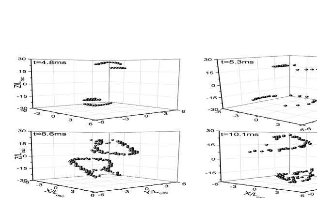
Figure 1: Typical examples of vortex germs. Here and in the following figures the time of the trap modulation is marked.

(iii) Vortex rings. After around $10$ ms, instead of the vortex germs, there appear well defined pairs of vortex rings, with vorticity $\pm 1$. Typical examples of vortex rings are illustrated by Fig. 2, where the modulation time is also marked. The rings do not move, except exhibiting small oscillations. The ring lifetime, after switching off pumping, is about $0.1$ s.

(iv) Vortex lines. Continuing pumping energy into the system leads, after about $15$ ms, to the formation of pairs of straight vortex lines, with vorticity $\pm 1$, directed along the $z$-axis, as is demonstrated in Fig. 3. The lines randomly move, probably, due to the Magnus force. The vortex lifetime, after switching off pumping, is about $0.2$ s.

(v) Deformed vortices. The longer perturbation, after around $17$ ms, starts strongly deforming vortex lines, making them not straight and chaotically directed. The lifetime of the deformed vortices is close to that of the straight vortex lines.

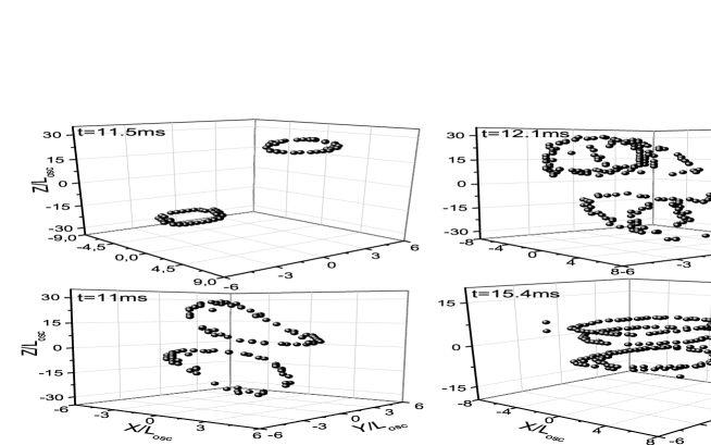
Figure 2: Typical examples of vortex rings.

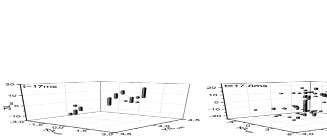
Figure 3: Typical examples of straight vortex lines directed along the $z$ axis.

(vi) Vortex turbulence. After about $25$ ms, the number of deformed vortices sharply increases and they form a randomly oriented vortex tangle, typical of the Vinen turbulence [2, 3, 4, 30]. The total regime of vortex turbulence can be subdivided onto the stages of developing turbulence, developed turbulence, and decaying turbulence. The stage of developed vortex turbulence is demonstrated in Fig. 4. The regime of vortex turbulence can be classified as such, since it exhibits several features typical of quantum turbulence: First, there appears a random tangle of vortices, corresponding to the definition of quantum turbulence by Feynman [31]. Second, being released from the trap, the atomic cloud expands isotropically, which is typical of Vinen turbulence [32]. Third, the column-integrated radial momentum distribution obeys a power low $n_{r}(k)\propto k^{-\gamma}$ in the range [4] $k_{min}<k<k_{max}$, with $k_{min}\approx\pi/\xi$ and $k_{max}\approx 2\pi/\xi$, which is a key quantitative expectation for an isotropic turbulent cascade [33], and which has been observed for turbulence of trapped atomic clouds [10, 34]. We have found that in this range $0.284\times 10^{6}\rm{cm}^{-1}<k<0.568\times 10^{6}\rm{cm}^{-1}$, the slope of $n_{r}(k)$ is $\gamma\approx 1.7$, which is close to $\gamma\approx 2$ found in the experiment [34] accomplished for the same system with the same parameters.

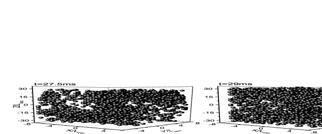
Figure 4: Developed vortex turbulence.

(vii) Grain turbulence. The regime of decaying vortex turbulence, after approximately $40$ ms, is followed by the state, where there are practically no vortices, but the whole trap is filled by randomly distributed in space dense Bose-condensed droplets, or grains, surrounded by a rarified gas. The droplets are almost spherical, with the radii $(0.5-2.5)\times 10^{-5}$ cm. The typical droplet radius of $1.5\times 10^{-5}$ cm is close to the coherence length, as it should be. The density inside a droplet is $20-100$ times higher than in the surrounding gas. The lifetime of a grain, after switching off pumping, is about $0.01$ s. During this time, droplets chaotically move in space, then some of them disappear, while new appear. The droplet lifetime is much longer that the local equilibration time $t_{loc}=m/\hbar\rho a_{s}=0.8\times 10^{-3}$ s. Hence the droplets are metastable objects. Each droplet is coherent, having a constant phase, while in the surrounding the phase is random. Such a state can be treated as a heterophase mixture of Bose-condensed droplets immersed into the gas of uncondensed atoms [35, 36]. The density snapshot for a radial cross-section, comparing the state of grain turbulence with the equilibrium unperturbed condensate and with the following state of wave turbulence is shown in Fig 5. It is important to stress that the granulated state of matter, to be classified as such, has to satisfy the following criteria: (1) the typical size of each droplet, representing a coherent formation, is of the order of the healing length; (2) the phase inside a droplet is constant, as it should be for a coherent object; (3) the phase in the space around a droplet is random, so that the coherent droplets are separated from each other by incoherent surrounding; (4) the lifetime of a droplet is much longer than the local equilibration time, which defines the droplets as metastable objects; (5) to look really as a droplet inside a rarified gas, the density inside a droplet is to be much larger than that of its incoherent surrounding. If these criteria are not satisfied, the matter cannot be classified as granulated. In our case all these criteria hold true.

(viii) Wave turbulence. Increasing perturbation by the trap modulation destroys Bose-condensed droplets after about $150$ ms and the system transfers into the state of wave turbulence [37, 38]. The state is a collection of small-amplitude waves, with the sizes $(0.5-1.5)\times 10^{-4}$ cm and with the density only about $3$ times larger than the density of their surrounding. There is no coherence either inside a wave or between them, since the phase is random. Strictly speaking, the transition from the regime of grain turbulence to wave turbulence is a gradual crossover, with more and more destroyed coherence. The latter becomes practically completely destroyed, so that the phase is everywhere chaotic, at about $150$ ms. The density snapshot of the state is demonstrated in Fig. 5.

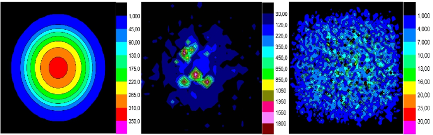
Figure 5: Density snapshots of equilibrium condensate (left plot), grain turbulence (middle plot), and wave turbulence (right plot). The legends on the right-hand side of each plot show the density in units of $1/l_{0}^{3}$.

3 Quantitative characterization of nonequilibrium states

In this way, by injecting energy into the trap, we create different nonequilibrium states with various topological defects, finally transforming an initially equilibrium Bose-condensed system into the state, where Bose-Einstein condensate is completely destroyed. This process, being opposite to equilibration, can be treated as inverse Kibble-Zurek scenario [14]. The remaining problem is how it would be possible to quantitatively characterize the nonequilibrium states arising during this disequilibration process. Several characteristics can be suggested for such a characterization.

First of all, it is possible to check that the energy, pumped into the system, goes almost completely to the increase of kinetic energy [14]. The latter can be connected with the effective temperature. Therefore, it is natural to define the effective temperature, in energy units, by the increase of kinetic energy per atom from the initial value $E_{kin}(0)$ to its value $E_{kin}(t)$ at time $t$,

$$T_{eff}(t)\equiv\frac{2}{3}\;[E_{kin}(t)-E_{kin}(0)]\;.$$ (2)

Note that this expression is written in energy units. To get the units of Kelvin temperatures, one has to divide Eq. (2) by the Boltzmann constant $k_{B}$.

The other idea comes to our mind if we remember that the phenomenon of turbulence is very general, arising in different media. Stochastic vortex tangles exist in many physical fields of similar systems of highly disordered sets of one-dimensional topological objects. As examples, it is possible to mention global cosmic strings, the flux tubes in superconductors, dislocations in solids, linear topological defects in liquid crystals and polymer chains, turbulent effects in quark-gluon plasma and neutron stars (see discussion in reviews [4, 5]). The emergence of multiple random filamentation in a high-intensity, ultrashort laser beam, due to optical turbulence, has been observed [39, 40, 41, 42]. The phenomenon of photon turbulence, or optical turbulence, also occurs in high-Fresnel-number lasers, where the increase of the laser Fresnel number leads to the appearance of turbulent photon filamentation [43, 44, 45].

That is, the Fresnel number can serve as a characteristic of the system state. For lasers, with wavelength $\lambda$, radius $R$, and length $L$, the Fresnel number is $F=\pi R^{2}/\lambda L$. For atomic traps, the role of radius is played by the oscillator length $R=l_{r}=\sqrt{\hbar/m\omega_{r}}$, while the axial length is given by $L=2l_{z}=2\sqrt{\hbar/m\omega_{z}}$. As the wavelength, it is natural to accept the length $\lambda_{T}=\hbar\sqrt{2\pi/mT_{eff}}$. Thus, the effective Fresnel number can be written as

$$F=\frac{\pi R^{2}}{\lambda_{T}L}=\sqrt{\frac{\pi\alpha T_{eff}}{8\hbar\omega_{r}}}\;,$$ (3)

where $\alpha$ is the aspect ratio.

It is also possible to recollect that turbulence is connected with such a characteristic as the Mach number $M=v/c$, in which $v$ is the velocity of a moving object and $c$ is sound velocity [22]. For atomic systems, the velocity of an atom can be represented as $v=\sqrt{2E_{kin}/m}$ and the sound velocity can be written as $c=(\hbar/m)\sqrt{4\pi\rho a_{s}}$, where $\rho$ is the density at the trap center. Hence the effective Mach number takes the form

$$M=\sqrt{\frac{2E_{kin}}{mc^{2}}}=\frac{1}{\hbar}\;\sqrt{\frac{mE_{kin}}{2\pi\rho a_{s}}}\;.$$ (4)

The first expression here is what is called turbulence Mach number [22].

In general, the Mach number shows the relation between the object velocity and the speed of sound. Considering an obstacle, such as, e.g., laser beam moving through the fluid, is a particular case. In our study the Mach number characterizes the relation between the characteristic velocity of atoms and the speed of sound. The Mach number we introduce describes how a particle moves inside the system. In that sense, a particle is also an effective moving object, similar to an obstacle. So, the suggested definition is a straightforward generalization of the standard Mach number. Recall that cold atoms, we consider, are not thermal. Their speed has no connection with thermal motion, but reflects the speed due to quantum kinetic energy. In the case of cold atoms, kinetic energy is caused by quantum motion, while for classical systems kinetic energy is really thermal. This makes the principal difference between quantum and classical systems.

In Fig. 6, we illustrate the classification of all nonequilibrium states, we have found, by means of the effective temperature, Fresnel number, and Mach number. It is interesting that the regime of wave turbulence, where all coherence is destroyed, corresponds to the effective temperature $T_{eff}=23.5\hbar\omega_{r}$, which practically coincides with the temperature $T_{c}=23.8\hbar\omega_{r}$ of Bose-Einstein condensation of ⁸⁷Rb in the considered setup. The critical temperature in Kelvin degrees is $2.4\times 10^{-7}$ K. The developed wave turbulence implies that, although the system is yet quantum, but there is no coherence, as it should be above the condensation temperature. The Fresnel and Mach numbers vary between small values close to zero, in weak nonequilibrium, to the values close to one, in wave turbulence.

Note that for a strongly nonequilibrium system, the standard notion of temperature is not defined, but one can speak only about an effective temperature, as we do. The closeness of the effective temperature at the moment, when the coherence is destroyed by perturbations, to the Bose condensation temperature implies that coherence can be destroyed either by heating of an equilibrium system or by injecting kinetic energy into a nonequilibrium system, for which heating has no meaning.

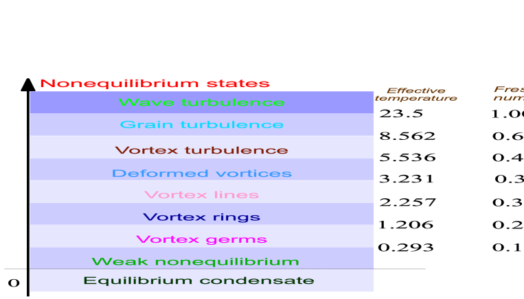
Figure 6: Sequence of nonequilibrium states observed in computer modeling, characterized by the effective temperature $T_{eff}$ (in units of $\hbar\omega_{r}$), Fresnel number, and Mach number.

4 Conclusion

In conclusion, we have accomplished a detailed numerical investigation of nonequilibrium states arising in the process of perturbing the Bose-Einstein condensate of trapped atoms by an alternating potential. Starting from an equilibrium condensate, we generate the state of weak nonequilibrium, the states with vortex germs, vortex rings, vortex lines, and with deformed vortices, vortex turbulence, grain turbulence, and wave turbulence. The characterization of the nonequilibrium states is suggested by means of effective temperature, Fresnel number, and Mach number. The latter are well defined quantities expressed through the known system parameters and kinetic energy that can be straightforwardly calculated numerically as well as measured experimentally. The overall physical picture remains the same, if the perturbation parameters are varied. This is because the main characteristics of the states depend on the injected kinetic energy that can be shown [12, 13, 14] is proportional to the product $A\omega t$ of the modulation amplitude $A$, modulation frequency $\omega$, and modulation time $t$. So, the same amount of kinetic energy can be injected into the trap by increasing the modulation amplitude, but decreasing the modulation time or modulation frequency.

The suggested characteristics can be used for the traps of any geometry and for any type of cold atoms. The main definitions of the effective temperature, Fresnel number, and Mach number remain the same, although the expressions for the system sizes $R$ and $L$, as well as for the sound velocity $c$, can be different, depending on the trap geometry and system parameters. For example, in the case of a cylindrical box [10], the system sizes are given by the radius $R$ and length $L$ of the box.

It is important to emphasize that the characterization of nonequilibrium states, proposed in the present paper is very general and can be employed for all systems for which such straightforward quantities as kinetic energy and the system sizes can be defined. These quantities, as is evident, can be defined for practically any experimental scheme. The suggested characteristics can be measured in experiments, provided kinetic energy can be measured. The latter can be found by measuring the momentum distribution $n({\bf k})$, as has been done in the experiments with trapped atoms [34, 46], after which the kinetic energy is straightforwardly obtained by integrating over momenta of the expression $(k^{2}/2m)n({\bf k})$.

The authors are grateful to M. Tsubota for discussions and advice. One of the authors (A.N. N.) would like to thank CNPq (project 150343/2016-7) for post-doctoral fellowship and BLTP JINR for generous access to computational facilities. The other author (V.I.Y.) appreciates discussions with E.P. Yukalova. The authors acknowledge useful cooperation with Center CEPOF and support from FAPESP (CEPID).

References

- [1] Vinen W F and Niemela J J 2002 J. Low Temp. Phys. 128 167
- [2] Vinen W F 2006 J. Low Temp. Phys. 145 7
- [3] Vinen W F 2010 J. Low Temp. Phys. 161 419
- [4] Tsubota M, Kobayashi M and Takeuchi, H 2013 Phys. Rep. 522 191
- [5] Nemirovskii S K 2013 Phys. Rep. 524 85
- [6] Wilson K E, Samson E C, Newman Z I, Neely T W and Anderson B P 2013 Ann. Rev. Cold At. Mol. 1 261
- [7] Tsatsos M C, Tavares P E S, Cidrim A, Fritsch A R, Caracanhas M A, Dos Santos F E A, Barenghi C F, and Bagnato V S 2016 Phys. Rep. 622 1
- [8] Yukalov V I, Yukalova E P and Bagnato V S 1997 Phys. Rev. A 56 4845
- [9] Yukalov V I, Yukalova E P and Bagnato V S 2002 Phys. Rev. A 66 043602
- [10] Navon N, Gaunt A L, Smith R P and Hadzibabic Z 2016 Nature 532 72
- [11] Bagnato V S and Yukalov V I 2013 Prog. Opt. Sci. Photon. 1 377
- [12] Yukalov V I, Novikov A N and Bagnato V S 2014 Laser Phys. Lett. 11 095501
- [13] Yukalov V I, Novikov A N and Bagnato V S 2015 J. Low Temp. Phys. 180 53
- [14] Yukalov V I, Novikov A N and Bagnato V S 2015 Phys. Lett. A 379 1366
- [15] Salmon R L 1998 Lectures on Geophysical Fluid Dynamics (Oxford: Oxford University)
- [16] Donnelly R J 1991 Quantized Vortices in Helium II (Cambridge: Cambridge University)
- [17] Barenghi C F 2008 Physica D 237 2195
- [18] Reeves M T, Billam T P, Anderson B P and Bradley S A 2015 Phys. Rev. Lett. 114 155302
- [19] Kwon W L, Kim J H, Seo S W and Shin Y 2016 Phys. Rev. Lett. 117 245301
- [20] Sasaki K, Suzuki N and Saito H 2010 Phys. Rev. Lett. 104 150404
- [21] Stagg G W, Parker N G and Barenghi C F 2014 J. Phys. B 47 095304
- [22] Smits A J and Dussauge J P 2006 Turbulent Shear Layers in Supersonic Flow (New York: Springer)
- [23] Inouye S, Chikkatur A P, Stamper-Kurn D M, Stenger J, Pritchard D E and Ketterle W 1999 Science 285 571
- [24] Pethick C J and Smith H 2008 Bose-Einstein Condensate in Dilute Gases (Cambridge: Cambridge University)
- [25] Shiozaki R F, Telles G D, Yukalov V I and Bagnato V S 2011 Laser Phys. Lett. 8 393
- [26] Seman J A, Henn E A L, Shiozaki R F, Roati G, Poveda-Cuevas F J, Magalhães K M F, Yukalov V I, Tsubota M, Kobayashi M, Kasamatsu K and Bagnato V S 2011 Laser Phys. Lett. 8 691
- [27] Birman J L, Nazmitdinov R G and Yukalov V I 2013 Phys. Rep. 526 1
- [28] Novikov A N, Yukalov V I and Bagnato V S 2015 J. Phys. Conf. Ser. 594 012040
- [29] Kobayashi M and Tsubota M 2005 J. Phys. Soc. Jap. 74 3248
- [30] Cidrim A, White A C, Allen A J, Bagnato V S and Barenghi C F 2017 Phys. Rev. A 96 023617
- [31] Feynman R P 1955 in Progress in Low Temperature Physics vol. 1, p. 17 (Amsterdam: North-Holland)
- [32] Caracanhas M, Fetter A, Baym G, Muniz S and Bagnato V S 2013 J. Low Temp. Phys. 170 133
- [33] Zakharov V E, Lvov V S and Falkovich G 1992 Kolmogorov Spectra of Turbulence (Berlin: Springer)
- [34] Thompson K J, Bagnato G G, Telles G D, Caracanhas M A, Dos Santos F E A and Bagnato V S 2014 Laser Phys. Lett. 11 015501
- [35] Yukalov V I 1991 Phys. Rep. 208 395
- [36] Yukalov V I 2003 Int. J. Mod. Phys. B 17 2333
- [37] Nazarenko S 2011 Wave Turbulence (Berlin: Springer)
- [38] Fujimoto K and Tsubota M 2015 Phys. Rev. A 91 053620
- [39] Berge L, Skupin S, Lederer F, Mejean G, Yu J, Kasparian J, Salmon E, Wolf J P, Rodriguez M, Wöste L, Bourayou R and Sauerbrey R 2004 Phys. Rev. Lett. 92 225002
- [40] Henin S, Petit Y, Kasparian J, Wolf J P, Jochmann A, Kraft S D, Bock S, Schramm U, Sauerbrey R, Nakaema W M, Stelmaszczyk K, Rohwetter P, Wöste L, Soulez C L, Mauger S, Berge L and Skupin S 2010 Appl. Phys. B 100 77
- [41] Loriot V, Bejot P, Ettoumi W, Petit Y, Kasparian J, Henin S, Hertz E, Lavorel B, Faucher O and Wolf J P 2011 Laser Phys. 21 1319
- [42] Ettoumi W, Kasparian J and Wolf J P 2015 Phys. Rev. Lett. 114 063903
- [43] Yukalov V I 2000 Phys. Lett. A 278 30
- [44] Yukalov V I and Yukalova E P 2000 Phys. Part. Nucl. 31 561
- [45] Yukalov V I 2014 Laser Phys. 24 094015
- [46] Bahrami A, Tavares P E S, Fritsch A R, Tonin Y R, Telles G D, Bagnato V S and Henn E A L 2015 J. Low Temp. Phys. 180 126