Mechanism for unconventional superconductivity in the hole-doped
Rashba-Hubbard model

Abstract

Motivated by the recent resurgence of interest in topological superconductivity, we study superconducting pairing instabilities of the hole-doped Rashba-Hubbard model on the square lattice with first- and second-neighbor hopping. Within the random phase approximation we compute the spin-fluctuation mediated paring interactions as a function of filling. Rashba spin-orbit coupling splits the spin degeneracies of the bands, which leads to two van Hove singularities at two different fillings. We find that for a doping region in between these two van Hove fillings the spin fluctuations exhibit a strong ferromagnetic contribution. Because of these ferromagnetic fluctuations, there is a strong tendency towards spin-triplet $f$-wave pairing within this filling region, resulting in a topologically nontrival phase.

Topological superconductors (TSCs) have attracted great interest recently due to their potential use for quantum information technology and novel superconducting devices Chiu et al. (2016); Hasan and Kane (2010); Qi and Zhang (2011); Schnyder et al. (2008); Schnyder and Brydon (2015); Sato and Ando (2016). Many interesting topological phases, such as the chiral $p$-wave state Read and Green (2000), are realized in superconductors with odd-parity spin-triplet pairing. However, until now only a few material systems have been discovered which show spin-triplet superconductivity Kallin and Berlinsky (2016); Maeno et al. (2012); Smidman et al. (2017), since spin-singlet pairing is in most cases the dominant pairing channel. There are two types of TSCs with triplet pairing: intrinsic and artificial ones. While the former type arises as an intrinsic property of the material, the latter is artificially engineered in heterostructures by proximity coupling to an $s$-wave superconductor Fu and Kane (2008). Intrinsic TSCs have the advantage that the topological phase exists in the entire volume of the material, and not just at an interface of a heterostructure. In recent years it has become clear that strong spin-orbit coupling (SOC) is conducive to triplet superconductivity Yanase and Sigrist (2007, 2008); Yokoyama et al. (2007). Indeed, most candidate materials for intrinsic TSCs, such as Sr₂RuO₄ Kallin and Berlinsky (2016); Maeno et al. (2012), CePt₃Si Smidman et al. (2017), and Cu_xBi₂Se₃ Hor et al. (2010); Sasaki et al. (2011), contain heavy elements with strong spin-orbit interactions. Unfortunately, the strongly correlated TSCs Sr₂RuO₄ and CePt₃Si have a rather low $T_{c}$ of $\lesssim 1~{}K$, while the pairing symmetry of the weakly correlated TSC Cu_xBi₂Se₃ is still under debate Levy et al. (2013); Brydon et al. (2014). Therefore, the search for new intrinsic TSCs remains an important goal.

Parallel to these developments, MBE fabrication of oxide and heavy-fermion superlattices has seen great progress Chakhalian et al. (2007); Reyren et al. (2007); Mizukami et al. (2011); Shimozawa et al. (2014). An important distinguishing feature of epitaxial superlattices is their high tunability. That is, carrier density, Fermi surface (FS) topology, as well as SOC can be tuned by modulating the layer thickness or by applying electric fields Caviglia et al. (2008); Shimozawa et al. (2014). Remarkably, some of these superlattices show unconventional superconductivity with a fairly high-transition temperature. One example is the heavy-fermion superlattice CeCoIn₅/YbCoIn₅ Mizukami et al. (2011); Shimozawa et al. (2014), in which magnetic fluctuations Stock et al. (2008) lead to superconductivity below $T_{\textrm{c}}\simeq 2$ K. Modulating the layer thicknesses in this superlattice breaks the inversion symmetry, which induces Rashba spin-orbit interactions. Interestingly, the strength of the Rashba SOC can be controlled by the width of the YbCoIn₅ block layers. Strong Rashba interaction drastically alters the FS topology by splitting the spin degeneracy. This in turn is favorable for triplet superconductivity, provided that the pairing mechanism allows for it. As is known from extensive theoretical works on cuprate superconductors Rømer et al. (2015); Scalapino et al. (1986); Hlubina (1999), the shape and topology of the FS strongly influence the relative strengths of different pairing channels. In order to optimize the layer thickness modulation in CeCoIn₅/YbCoIn₅ for triplet superconductivity, it is therefore important to understand the detailed interdependence among Rashba SOC, FS topology, and superconducting pairing symmetry.

Motivated by these considerations, we analyze in this Letter superconducting pairing instabilities of the hole-doped Rashba-Hubbard model, which describes the essential features of many strongly correlated materials with Rashba SOC Yokoyama et al. (2007); Yanase and Sigrist (2007, 2008); Meza and Riera (2014). Focusing on the square lattice with first- and second-neighbor hopping, $t$ and $t^{\prime}$, we compute the spin-fluctuation-mediated pairing interaction as a function of filling. For this purpose we use the random phase approximation (RPA), which is known to qualitatively capture the essential physics, at least within weak coupling Yanase and Sigrist (2007, 2008); Yokoyama et al. (2007); Rømer et al. (2015); Scalapino et al. (1986); Hlubina (1999). Finite SOC splits the energy bands leading to two van Hove singularities at the fillings $n_{vH_{1}}$ and $n_{vH_{2}}$. Remarkably, we find that in a doping region in between these two van Hove fillings, there exist strong ferromagnetic (FM) spin fluctuations (Figs. 1 and 2). Due to these FM fluctuations there is a strong tendency towards spin-triplet $f$-wave pairing in this filling region, while the pairing channels of $d$-wave type (Fig. 3) are of the same order or subdominant.

Model and Method.— The Rashba-Hubbard model on the square lattice is given

$$H=\sum_{\bf k}{\psi}^{\dagger}_{\bf k}\hat{h}({\bf k})\psi^{\ }_{{\bf k}}+U\sum_{{\bf k},{\bf k^{\prime}},{\bf q}}c^{\dagger}_{{\bf k}\uparrow}c_{{\bf k}+{\bf q}\uparrow}c^{\dagger}_{{\bf k^{\prime}}\downarrow}c_{{\bf k^{\prime}}-{\bf q}\downarrow},$$ (1)

where $U$ is the local Coulomb repulsion, $\hat{h}({\bf k})=\left(\varepsilon_{\bf k}\tau_{0}+{\bf g}_{\bf k}\cdot\bm{\tau}\right)$, and $\psi_{\bf k}=(c_{{\bf k}\uparrow},c_{{\bf k}\downarrow})^{T}$. Here, $\bm{\tau}=(\tau_{1},\tau_{2},\tau_{3})^{T}$ are the three Pauli matrices, and $\tau_{0}$ stands for the $2\times 2$ unit matrix. The band energy $\varepsilon_{\bf k}=-2t(\cos k_{x}+\cos k_{y})+t^{\prime}\cos k_{x}\cos k_{y}-\mu$ contains both first- and second-neighbor hopping, $t$ and $t^{\prime}$, respectively, and is measured relative to the chemical potential $\mu$. The vector ${\bf g}_{\bf k}$ describes Rashba SOC with ${\bf g}_{\bf k}=V_{\textrm{so}}(\partial\varepsilon_{\bf k}/\partial k_{y},-\partial\varepsilon_{\bf k}/\partial k_{x},0)$ and the coupling constant $V_{\textrm{so}}$. For our numerical calculations we set $t=1$, $t^{\prime}=0.3$, and $V_{\textrm{so}}=0.5$, and focus on the hole-doped case with filling $0.4<n<1$. We have checked that other parameter choices do no qualitatively change our findings. The presence of Rashba SOC splits the electronic dispersion $\varepsilon_{\bf k}$ into negative- and positive-helicity bands with energies $E_{\bf k}^{1}=\varepsilon_{\bf k}-\left|{\bf g}_{\bf k}\right|$ and $E_{\bf k}^{2}=\varepsilon_{\bf k}+\left|{\bf g}_{\bf k}\right|$, respectively. Both spin-split bands exhibit van Hove singularities at ${\bf k}=(\pi,0)$ and symmetry related points. For our parameter choice the corresponding van Hove fillings occur at $n_{vH_{1}}\simeq 0.87$ and $n_{vH_{2}}\simeq 0.65$, see inset of Fig. 2.

The first term of Eq. 1 defines the bare $2\times 2$ fermionic Greens function in the spin basis

$$G^{(0)}_{\sigma_{1}\sigma_{2}}({\bf k},i\nu_{n})=\left(\left[i\nu_{n}\tau_{0}-\hat{h}({\bf k})\right]^{-1}\right)_{\sigma_{1}\sigma_{2}},$$ (2)

where $\nu_{n}=2n\pi/\beta$ is the fermionic Matsubara frequency. For $U=0$ the bare spin susceptibility can be expressed in terms of $G^{(0)}$ as

$$\chi^{(0)}_{\sigma_{1}\sigma_{2}\sigma_{3}\sigma_{4}}({\bf q},i\omega_{l})=\sum_{{\bf k},i\nu_{n}}G^{(0)}_{\sigma_{1}\sigma_{2}}({\bf k},i\nu_{n})G^{(0)}_{\sigma_{3}\sigma_{4}}({\bf k}+{\bf q},i\nu_{n}+i\omega_{l}),$$ (3)

where $\omega_{l}=2l\pi/\beta$ is the bosonic Matsubara frequency. Within the RPA  Yanase and Sigrist (2007, 2008) the dressed spin susceptibility $\chi_{\sigma_{1}\sigma_{2}\sigma_{3}\sigma_{4}}({\bf q},i\omega_{l})$ is computed as

$$\hat{\chi}({\bf q},i\omega_{l})=\left[\mathbbm{1}-\hat{\chi}^{(0)}({\bf q},i\omega_{l})\hat{U}\right]^{-1}\hat{\chi}^{(0)}({\bf q},i\omega_{l}).$$ (4)

In Eq. (4) the sixteen components of $\chi_{\sigma_{1}\sigma_{2}\sigma_{3}\sigma_{4}}$ and $\chi^{(0)}_{\sigma_{1}\sigma_{2}\sigma_{3}\sigma_{4}}$ are stored in the $4\times 4$ matrices $\hat{\chi}$ and $\hat{\chi^{(0)}}$, respectively, and the $4\times 4$ coupling matrix $\hat{U}$ is antidiagonal, see the Supplemental Material (SM) sup for details.

The spin fluctuations described by Eq. (4) can lead to an effective interaction that combines two electrons into a Cooper pair. As in Refs. Rømer et al., 2015; Scalapino et al., 1986, it is necessary to distinguish between the interaction for same [$V_{\textrm{same}}^{\textrm{eff}}({\bf k},{\bf k^{\prime}})$] and for opposite [$V_{\textrm{opp}}^{\textrm{eff}}({\bf k},{\bf k^{\prime}})$] spin projections between two electrons with momentum ${\bf k}$ and ${\bf k^{\prime}}$foo (a), which are given in the spin basis by

$$V^{\textrm{eff}}_{\textrm{same}}({\bf k},{\bf k^{\prime}}) = U^{2}\chi_{\sigma\sigma\sigma\sigma}({\bf k-k^{\prime}}),$$ (5a)

$$V^{\textrm{eff}}_{\textrm{opp}}({\bf k},{\bf k^{\prime}}) = U^{2}\chi_{\sigma\bar{\sigma}\bar{\sigma}\sigma}({\bf k-k^{\prime}})+U^{2}\chi_{\sigma\sigma\bar{\sigma}\bar{\sigma}}({\bf k+k^{\prime}}),\quad$$ (5b)

respectively. In weak coupling we can define for each pairing channel $i$ a dimensionless pairing strength as Frigeri et al. (2006); Dolgov and Golubov (2008); Dolgov et al. (2009); Hirschfeld et al. (2011)

$$\lambda_{i}^{\alpha\beta}=-\frac{{\int}_{\textrm{FS}_{\alpha}}\frac{dk}{v^{\alpha}_{\textrm{F}}(k)}{\int}_{\textrm{FS}_{\beta}}\frac{dk^{\prime}}{v^{\beta}_{\textrm{F}}(k^{\prime})}\eta_{i}(k)V_{\textrm{s}/\textrm{t}}^{\textrm{eff}}(k,k^{\prime})\eta_{i}(k^{\prime})}{2\pi^{2}{\int}_{\textrm{FS}_{\beta}}\frac{dk^{\prime}}{v^{\beta}_{F}(k^{\prime})}\left[\eta_{i}(k^{\prime})\right]^{2}},$$ (6)

where $\alpha$ and $\beta$ label the FS sheets. The diagonal and off-diagonal elements of $\lambda_{i}^{\alpha\beta}$ represent intra- and inter Fermi surface pairing strengths, respectively. In Eq. (6), $k$ and $k^{\prime}$ are restricted to the Fermi sheets $\textrm{FS}_{\alpha}$ and $\textrm{FS}_{\beta}$, respectively, $v^{\alpha}_{\textrm{F}}({\bf k})=\left|\nabla_{\bf k}E^{\alpha}_{\bf k}\right|$ is the Fermi velocity, and $\eta_{i}(k)$ describes the $k$ dependence of each possible pairing symmetry, see SM sup . In the case of singlet pairing the effective interaction in Eq. (6) is solely due to scattering between electrons with opposite spins. For triplet pairing, however, both same- and opposite-spin scattering processes are possible. The effective superconducting coupling constant $\lambda_{i}^{\textrm{eff}}$ for a given pairing channel $i$ is given by the largest eigenvalue of the matrix $\lambda_{i}^{\alpha\beta}$ Dolgov and Golubov (2008). Hence, by numerically evaluating Eq. (6) for all possible channels $i$ we can identify the leading pairing instability as a function of filling and SOC strength.

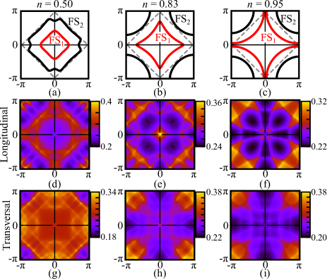
Figure 1: (a)-(c) Calculated Fermi surface topology and (d)-(i) static $\omega=0$ spin susceptibility for the fillings $n=0.50$, $n=0.83$, and $n=0.95$, with $t^{\prime}=0.3$, $V_{\textrm{so}}=0.5$, $T=0.01$, and $U=0.4$. The second and third rows show the longitudinal and transversal susceptibilities, $\chi_{\textrm{long}}=\chi_{\uparrow\uparrow\uparrow\uparrow}-\chi_{\uparrow\downarrow\downarrow\uparrow}$ and $\chi_{\textrm{trans}}=\chi_{\uparrow\uparrow\downarrow\downarrow}$, respectively (see SM sup ).

Spin susceptibility.— Before discussing superconductivity, let us first consider the static susceptibility in the paramagnetic state for intermediate coupling $U=0.4$ and $T=0.01$. While Figs. 1(d)-1(f) show the longitudinal susceptibility, Figs. 1(g)-1(i) show the transversal susceptibility for the fillings $n=0.5$, $n=0.83$, and $n=0.95$, respectively. As expected, and different to the case without SOC, the longitudinal and transversal susceptibilities show different spin texture. The FS topology for each filling is shown in Figs. 1(a)-1(c). The spin susceptibility shows large magnetic fluctuations, whose magnetic modulation vectors ${\bf q}$ depend strongly on filling $n$ and FS topology. Indeed, we observe an intricate interplay between FS topology and the structure of the spin susceptibility: For $n>n_{vH_{1}}$ the two spin-split FS sheets are hole-like and centered at $(\pi,\pi)$ [Fig. 1(c)], which results in a spin susceptibility with incommensurate anti-ferromagnetic modulation vector ${\bf q}=(\pi,\pi\pm\delta)$, see Figs. 1(f), and 1(i). For $n<n_{vH_{2}}$, on the other hand, both FS sheets are electron-like and centered at $\Gamma$ [Fig. 1(a)] leading to a longitudinal spin susceptibility with nearly commensurate anti-ferromagnetic ${\bf q}$ vector [Fig. 1(d)]. In between the two van Hove fillings, $n_{vH_{2}}<n<n_{vH_{1}}$, FS₁ is electron-like and centered at $\Gamma$, while FS₂ is hole-like and centered at $(\pi,\pi)$, see Fig. 1(b). Interestingly, within this filling range there exists a broad region, i.e., $0.76\lesssim n\lesssim n_{vH_{1}}$, where the dominant longitudinal fluctuations are ferromagnetic with ${\bf q}=(0,0)$, see Figs. 1(e) and 2.

Increasing the Hubbard interaction $U$ enhances the magnetic fluctuations and eventually drives the system into the magnetically ordered phase. In this process the modulation vector of the strongest fluctuations becomes the ordering wave vector of the ordered phase. The transition between paramagnetic and ordered phase occurs at the critical interaction strength $U_{c}$ with a given ordering wave vector where the susceptibility diverges. Although the transversal and longitudinal susceptibilities show different spin texture, both diverge simultaneously at the same ordering momentum, showing the non trivial feedback between them for finite SOC. Figure 2 displays the filling dependence of the critical interaction $U_{c}$ (red line). The color scale indicates the intensity of the ferromagnetic fluctuations in the longitudinal susceptibility relative to the (incommensurate) antiferromagnetic fluctuations. We observe that the ferromagnetic fluctuations are dominant in the filling range $0.76\lesssim n\lesssim n_{vH_{1}}$ and for $U$ within the range $0\leq U\lesssim 1.6$. These ferromagnetic fluctuations originate from the combined effect of finite SOC $V_{\textrm{so}}$ and finite $t^{\prime}$. As a matter of fact, for $V_{\textrm{so}}=0$ and $t^{\prime}\neq 0$ there is only one van Hove filling at $n_{vH}\sim 0.72$ (inset of Fig. 2), which separates commensurate antiferromagnetism [${\bf q}=(\pi,\pi)$] for $n>n_{vH}$ from incommensurate antiferromagnetism [${\bf q}=(\pi,\pi-\delta)$] for $n<n_{vH}$, and ferromagnetic fluctuations only occur in a narrow region around the van Hove filling $n_{vH}$ Rømer et al. (2015). For $t^{\prime}=0$ and $V_{\textrm{so}}\neq 0$ ferromagnetic fluctuations are absent Yokoyama et al. (2007). Different to the longitudinal susceptibility the transversal susceptibility shows ferromagnetic fluctuations only very close to the van Hove fillings $n_{vH_{1}}$ and $n_{vH_{2}}$ [Fig. S5 of the SM].

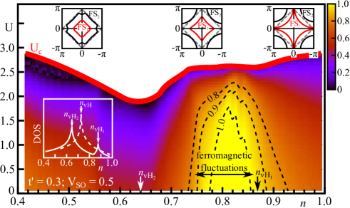
Figure 2: The critical interaction strength $U_{c}$ as a function of filling $n$ is indicated by the red line. The color scale represents the relative intensity of the ferromagnetic fluctuations in the longitudinal susceptibility. The inset shows the density of states versus filling for $V_{\textrm{so}}=0$ (dashed line) and $V_{\textrm{so}}=0.5$ (solid line).

Superconducting instabilities.— The discussed magnetic fluctuations can lead to superconducting pairing instabilities. We set the Hubbard interaction to $U=0.4<U_{c}$ and compute $\lambda_{i}^{\textrm{eff}}$ within the filling range $0.4<n<1$ for the lowest-harmonic pairing symmetries, as defined in Eq. (S11) of the SM. The resulting filling dependence of the pairing symmetries is presented in Fig. 3. Note that the weak coupling approach is more reliable away from the van Hove fillings. At the van Hove fillings $n_{vH_{i}}$, $\lambda_{i}^{\textrm{eff}}$ exhibits large jumps due to the divergent density of states foo (b), which is an artifact of the weak coupling approach. Let us examine the results of Fig. 3 separately for (i) $n>n_{vH_{1}}$, (ii) $n<n_{vH_{2}}$, and (iii) $n_{vH_{2}}<n<n_{vH_{1}}$:

(i) $n>n_{vH_{1}}$: For this filling region the singlet d${}_{x^{2}-y^{2}}$-wave pairing channel is dominant. This is due to large anti-ferromagnetic spin fluctuations that exist in the entire hole-doping range $1>n>n_{vH_{1}}$, similar to the case of $V_{\textrm{so}}=0$ Rømer et al. (2015). The subleading pairing solutions have $p$-wave and $f$-wave symmetry due to effective interactions with same spin projections. Notice that in contrast to the case for $V_{\textrm{so}}=0$ Rømer et al. (2015), here the pairing strength for same spin projections is different from opposite spin projections. While the tendency to superconductivity in the $f$-wave channel is strongly decreasing approaching half-filling, it is rather stable for the $p$-wave channel. Because Rashba SOC breaks inversion symmetry, we expect that in this filling range the pairing symmetry is an admixture of $d_{x^{2}-y^{2}}$-wave, $p$-wave, and $f$-wave Frigeri et al. (2004). However, since $\lambda^{\textrm{eff}}_{d_{x^{2}-y^{2}}}\gg\lambda^{\textrm{eff}}_{p/f}$, the $d_{x^{2}-y^{2}}$-wave channel is the leading one.

(ii) $n<n_{vH_{2}}$: In this filling region the $d_{xy}$-wave pairing is leading, while the $f$-wave and $p$-wave channels are subdominant. We ascribe this tendency towards $d_{xy}$-wave pairing, rather than $d_{x^{2}-y^{2}}$-wave, to the strong transversal spin fluctuations, which are peaked at $(\pi,0)$ and symmetry related points.

(iii) $n_{vH_{2}}<n<n_{vH_{1}}$: This is the most interesting region. Remarkably, we find that around the filling $n\simeq 0.78$ the triplet $f$-wave solution for same spin projections is the leading one, which we attribute to the strong ferromagnetic fluctuations that occur for this filling in the longitudinal susceptibility [cf. Figs. 1(e) and 2]. The subdominant pairing channels have $d_{x^{2}-y^{2}}$-wave and $d_{xy}$-wave form. Hence, due to broken inversion symmetry, the gap is expected to exhibit also $d$-wave admixture to the dominant $f$-wave harmonic. Although the weak coupling RPA approach underestimates the values of $\lambda_{i}^{\textrm{eff}}$, it nevertheless qualitatively captures the relative tendency to superconductivity in each channel. Different to the case for $V_{\textrm{so}}=0$  Rømer et al. (2015), where ferromagnetic fluctuations occur only very close to the van Hove filling and a singular behavior is found at this filling for triplet $f$-wave pairing, here triplet $f$-wave extends in a broad filling region. This fact rules out the possibility that the observed tendency towards $f$-wave pairing is an artifact of the van Hove singularity. Without second-neighbor hopping the triplet pairing component is always subdominant Yokoyama et al. (2007). Thus, our results offer a microscopic mechanism for the realization of triplet pairing with same spin projection, which was proposed on phenomenological grounds to be a candidate in non-centrosymmetric systems with strong SOC Frigeri et al. (2004).

To analyze the dominance of the triplet $f$-wave channel we show in Fig. 3(b) the dependence of $\lambda^{\textrm{eff}}_{i}$ on the interaction strength $U$ for $n=0.78$. We find that $\lambda^{\textrm{eff}}_{f}$ is the largest effective coupling for $0.0<U\lesssim 0.5$. This behavior is consistent with the result of Fig. 2 which shows that the ferromagnetic fluctuations become less and less dominant with increasing $U$. Before concluding, let us briefly discuss the contributions of the intra and inter FS scattering processes to the effective superconducting coupling. In Figs. 3(c) we present the filling dependence of the intra FS ($\lambda^{11}_{i}$ and $\lambda^{22}_{i}$) and the inter FS ($\lambda^{12}_{i}$) pairing strengths for the $f$-wave channel for same spin projections sup . We observe that the $f$-wave pairing is driven by intra FS processes within FS₂.

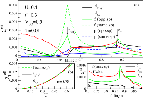
Figure 3: (a) Filling dependence of the superconducting couplings $\lambda_{i}^{\textrm{eff}}$, as determined from Eq. (6) for $U=0.4$, and for the lowest-harmonic pairing symmetries given by Eq. (S11). Here, we do not show the $s$-wave pairing channel, since it is highly suppressed (i.e., negative) for the entire hole-doping range. For the numerical evaluation of Eq. (6) we used $408$ Fermi momenta. (b) $\lambda^{\textrm{eff}}_{i}$ versus $U$ for the filling $n=0.78$. We present results up to $U=0.7$ to show the regime where $f$-wave is dominant. With increasing $U$ the curves increase monotonically, and $d$-wave becomes dominant while $f$-wave subdominant for $U\gtrsim 0.5$. Near the magnetic instability $U=U_{c}$ we find that $\lambda_{d}^{\textrm{eff}}\sim 0.2$ and $\lambda_{f}^{\textrm{eff}}\sim 0.15$. (c) Filling dependence of the intra and inter FS pairing strengths, $\lambda^{\alpha\alpha}_{i}$ and $\lambda^{\alpha\beta}_{i}$, for the $f$-wave channel with same spin projections.

Conclusions and implications for experiments.— We have studied superconducting instabilities of the hole-doped Rashba-Hubbard model with first- and second-neighbor hopping within a spin-fluctuation-mediated pairing scenario. Using an RPA approach, we have determined the pairing symmetry as a function of filling and have shown that there exists an interplay between FS topology, structure of the magnetic fluctuations, and pairing symmetry. In between the two van Hove fillings, close to $n\simeq 0.78$, the leading pairing solutions has triplet $f$-wave symmetry, which is driven by ferromagnetic fluctuations. Since within the spin fluctuation scenario the pairing symmetry is largely determined by the type of spin fluctuations, we expect that more sophisticated treatments, such as FLEX Yanase et al. (2003) or fRG Metzner et al. (2012), will confirm our RPA analysis. The tendency towards $f$-wave pairing near $n\simeq 0.78$ unavoidably leads to a topologically nontrivial state. The precise nature of this topological state depends on the detailed momentum structure of the gap. There are three possibilities: (i) The superconducting state is nodal with a dominant $f$-wave pairing symmetry and only small admixtures of $d$-wave and $p$-wave components. The point nodes of this superconducting state are topologically protected by a winding number, which gives rise to Majorana flat band edge states Schnyder and Brydon (2015). (ii) The superconducting state is fully gapped due to a sizable admixture of $d$-wave and $p$-wave components. In this case the superconducting state belongs to symmetry class DIII and exhibits helical Majorana edge states Chiu et al. (2016). (iii) The non-linear gap equation has a complex solution, yielding a time-reversal breaking triplet pairing state without nodes. This corresponds to a topological superconductor in symmetry class D, with chiral Majorana edge states Chiu et al. (2016). In closing we note that pair decoherence caused by impurity scattering is suppressed in all of the above three scenarios, due to the spin-momentum locking of the band structure foo (c).

Our findings provide a new mechanism for the creation of triplet superconductivity, which is relevant for non-centrosymmetric superconductors with strong SOC Smidman et al. (2017); Schnyder and Brydon (2015) and for oxide and heavy-fermion hybrid structures Chakhalian et al. (2007); Reyren et al. (2007); Mizukami et al. (2011); Shimozawa et al. (2014). It might be possible to realize the discussed $f$-wave state in CeCoIn₅/YbCoIn₅ hybrid structures Mizukami et al. (2011); Shimozawa et al. (2014), by an appropriate choice of layer thickness modulation. We hope that the present study will stimulate further experimental investigations along these directions.

Acknowledgments.— We thank M. Bejas, H. Nakamura, J. Riera, A. T.  Rømer, T. Yokoyama, and R. Zeyher for useful discussions. A.G. thanks the Max Planck Institute for Solid State Research in Stuttgart for hospitality and financial support.

In this supplemental material we give details of the derivation of the RPA spin susceptibility and the effective pairing interactions. We also present additional plots of the spin susceptibility and the pairing strengths $\lambda_{i}^{\textrm{eff}}$.

I I.   Derivation of the RPA spin susceptibility

Figure S1: The spin susceptibility $\chi_{\sigma_{1}\sigma_{2}\sigma_{3}\sigma_{4}}$ is calculated within RPA as a sum of bubbles and ladders. In the diagrams only external indices ($\sigma_{1},\sigma_{2},\sigma_{3}$, and $\sigma_{4}$) are indicated. Internal indices or omitted and are assumed to be summed over. Note that due to finite SOC the contributions from bubble and ladder diagrams are mixed, which is in contrast to the case without SOC Rømer et al. (2015); Scalapino et al. (1986).

Within the RPA the spin susceptibility $\chi_{\sigma_{1}\sigma_{2}\sigma_{3}\sigma_{4}}({\bf q},i\omega_{l})$ in the spin basis is obtained from an infinite sum of bubble and ladder diagrams, as shown in Fig. S1. The solid lines in the diagrams correspond to the bare $2\times 2$ fermionc propagator $G^{(0)}_{\sigma_{1}\sigma_{2}}({\bf k},i\nu_{n})$ [see Eq. (S2) and Fig. S2(a)] and the dashed lines are the bare vertex $U$ [see Fig. S2 (b)]. The bare susceptibility, represented by a single bubble in Fig. S1, is given by

$$\chi^{(0)}_{\sigma_{1}\sigma_{2}\sigma_{3}\sigma_{4}}({\bf q},i\omega_{l})=\sum_{{\bf k},i\nu_{n}}G^{(0)}_{\sigma_{1}\sigma_{2}}({\bf k},i\nu_{n})G^{(0)}_{\sigma_{3}\sigma_{4}}({\bf k}+{\bf q},i\nu_{n}+i\omega_{l}),$$ (S1)

with $\omega_{l}$ the bosonic Matsubara frequency, and

$$G^{(0)}_{\sigma_{1}\sigma_{2}}({\bf k},i\nu_{n})=\left(\left[i\nu_{n}\sigma_{0}-\hat{h}({\bf k})\right]^{-1}\right)_{\sigma_{1}\sigma_{2}}$$ (S2)

the $2\times 2$ bare Greens function with $\nu_{n}=(2n+1)\pi/\beta$ the fermionic Matsubara frequency. Arranging the sixteen matrix elements of $\chi^{(0)}_{\sigma_{1}\sigma_{2}\sigma_{3}\sigma_{4}}$ in a $4\times 4$ matrix,

$$\hat{\chi}^{(0)}=\left(\begin{array}[]{llll}\chi^{(0)}_{\uparrow\uparrow\uparrow\uparrow}&\chi^{(0)}_{\uparrow\downarrow\uparrow\uparrow}&\chi^{(0)}_{\uparrow\uparrow\downarrow\uparrow}&\chi^{(0)}_{\uparrow\downarrow\downarrow\uparrow}\\ \chi^{(0)}_{\uparrow\uparrow\uparrow\downarrow}&\chi^{(0)}_{\uparrow\downarrow\uparrow\downarrow}&\chi^{(0)}_{\uparrow\uparrow\downarrow\downarrow}&\chi^{(0)}_{\uparrow\downarrow\downarrow\downarrow}\\ \chi^{(0)}_{\downarrow\uparrow\uparrow\uparrow}&\chi^{(0)}_{\downarrow\downarrow\uparrow\uparrow}&\chi^{(0)}_{\downarrow\uparrow\downarrow\uparrow}&\chi^{(0)}_{\downarrow\downarrow\downarrow\uparrow}\\ \chi^{(0)}_{\downarrow\uparrow\uparrow\downarrow}&\chi^{(0)}_{\downarrow\downarrow\uparrow\downarrow}&\chi^{(0)}_{\downarrow\uparrow\downarrow\downarrow}&\chi^{(0)}_{\downarrow\downarrow\downarrow\downarrow}\end{array}\right)\;,$$ (S3)

the infinite sum in Fig. S1 can be expressed analytically as Yanase and Sigrist (2008)

$$\hat{\chi}({\bf q},i\omega_{l})=\left[I-\hat{\chi}^{(0)}({\bf q},i\omega_{l})\hat{U}\right]^{-1}\hat{\chi}^{(0)}({\bf q},i\omega_{l}),$$ (S4)

where the dressed $4\times 4$ matrix $\hat{\chi}$ contains the sixteen dressed susceptibilities arranged in similar form as in $\hat{\chi}^{(0)}$. The $4\times 4$ interaction matrix $\hat{U}$ in Eq. (S4) is off-diagonal with

$$\hat{U}=\left(\begin{array}[]{llll}0&0&0&U\\ 0&0&-U&0\\ 0&-U&0&0\\ U&0&0&0\end{array}\right)\;.$$ (S5)

Figure S2: (a) Diagram of the $2\times 2$ fermionic propagator, Eq. (S2). (b) Diagram of the four leg interaction vertex $U$, corresponding to the second term in Eq. (1) of the main text.

The longitudinal and transversal susceptibilities can be computed in terms of the matrix elements $\chi_{\sigma_{1}\sigma_{2}\sigma_{3}\sigma_{4}}$ as

$$\chi_{\textrm{long}}({\bf q},i\omega_{l})=\chi_{\uparrow\uparrow\uparrow\uparrow}({\bf q},i\omega_{l})-\chi_{\uparrow\downarrow\downarrow\uparrow}({\bf q},i\omega_{l})$$ (S6)

and

$$\chi_{\textrm{trans}}({\bf q},i\omega_{l})=\chi_{\uparrow\uparrow\downarrow\downarrow}({\bf q},i\omega_{l}),$$ (S7)

respectively. Note that the elements $(1,4)$ and $(4,1)$ of $\hat{U}$ enter in the bubble summation, while the elements $(2,3)$ and $(3,2)$ enter in the ladder summation in Fig. S1.

II II.   Derivation of the effective paring interactions

Figure S3: These diagrams depict the effective interactions for (a) opposite spin projections and (b) same spin projections.

The effective spin-fluctuation-mediated interaction can be computed within the random phase approximation (RPA)Rømer et al. (2015); Scalapino et al. (1986). It can be decomposed into same spin projections $V^{\textrm{eff}}_{\textrm{same}}({\bf k},{\bf k^{\prime}})$ and opposite spin projections $V^{\textrm{eff}}_{\textrm{opp}}({\bf k},{\bf k^{\prime}})$. The effective interaction for opposite spin has two contributions, as shown in Fig. S3(a), which can be written as

$$V^{\textrm{eff}}_{\textrm{opp}}({\bf k},{\bf k^{\prime}})=U^{2}\chi_{\sigma\bar{\sigma}\bar{\sigma}\sigma}({\bf k-k^{\prime}})+U^{2}\chi_{\sigma\sigma\bar{\sigma}\bar{\sigma}}({\bf k+k^{\prime}}).$$ (S8)

The effective interaction for same spin projections, on the other hand, has only one contribution [see Fig. S3(b)] and is expressed as

$$V^{\textrm{eff}}_{\textrm{same}}({\bf k},{\bf k^{\prime}})=U^{2}\chi_{\sigma\sigma\sigma\sigma}({\bf k-k^{\prime}}).$$ (S9)

Using these effective interactions and employing a standard BCS approach, focusing on temperatures $T$ close to $T_{\textrm{c}}$, we obtain the following linearized gap equations for the singlet (s) and triplet (t) channels in weak coupling

$$\Delta^{\textrm{s}/\textrm{t}}_{\alpha}(k)=\ln\left(\frac{1.13\,\omega_{\textrm{c}}}{T_{\textrm{c}}}\right)\sum_{\beta}\int_{\textrm{FS}_{\beta}}\frac{dk^{\prime}}{v^{\beta}_{\textrm{F}}(k^{\prime})}V_{\textrm{s}/\textrm{t}}^{\textrm{eff}}(k,k^{\prime})\Delta^{\textrm{s}/\textrm{t}}_{\beta}(k^{\prime}),$$ (S10)

where $\alpha,\beta=1,2$ label the FS sheets. Here, $k$ and $k^{\prime}$ are restricted to the Fermi sheets $\textrm{FS}_{\alpha}$ and $\textrm{FS}_{\beta}$, respectively, $v^{\alpha}_{\textrm{F}}({\bf k})=\left|\nabla_{\bf k}E^{\alpha}_{\bf k}\right|$ is the Fermi velocity, and $\omega_{\textrm{c}}$ denotes the cutoff frequency, which is given by the energy scale of the magnetic fluctuations. In the case of singlet pairing the effective interaction $V_{\textrm{s}}^{\textrm{eff}}$ in Eq. (S10) originates only from scattering between electrons with opposite spins, i.e., we set $V_{\textrm{s}}^{\textrm{eff}}(k,k^{\prime})=V^{\textrm{eff}}_{\textrm{opp}}(k,k^{\prime})$. For triplet pairing, both equal- and opposite-spin scattering processes can yield a solution to Eq. (S10). We therefore solve Eq. (S10) for both $V_{\textrm{t}}^{\textrm{eff}}(k,k^{\prime})=V^{\textrm{eff}}_{\textrm{same}}(k,k^{\prime})$ and $V_{\textrm{t}}^{\textrm{eff}}(k,k^{\prime})=V^{\textrm{eff}}_{\textrm{opp}}(k,k^{\prime})$.

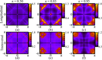
Figure S4: Longitudinal and transverse RPA spin susceptibilities for the fillings $n=0.50$, $n=0.83$, and $n=0.95$, respectively, with $t^{\prime}=0.3$, $V_{\textrm{so}}=0.5$, $k_{\textrm{B}}T=0.01$, and $U=2.2$. The corresponding plots for $U=0.4$ are shown in Fig. 1 of the main text.

In order to determine the symmetries of the pairing instabilities, we decompose the superconducting order parameter into an amplitude and a dimensionless symmetry function $\eta_{i}(k)$ for each pairing channel $i$. That is, we write $\Delta^{\textrm{s}/\textrm{t}}_{\alpha}(k)=\Delta_{\alpha}\eta_{i}(k)$, where $\eta_{i}(k)$ describes the $k$ dependence of each possible pairing symmetry on the square lattice:

$$\eta_{s}=1,\;\eta_{d_{x^{2}-y^{2}}}=\cos k_{x}-\cos k_{y},\;\eta_{d_{xy}}=\sin k_{x}\sin k_{y},$$

$$\eta_{p}=\sin k_{x},\;\textrm{and}\;\;\eta_{f}=(\cos k_{x}-\cos k_{y})\sin k_{x}.$$ (S11)

Inserting the decomposition $\Delta^{\textrm{s}/\textrm{t}}_{\alpha}(k)=\Delta_{\alpha}\eta_{i}(k)$ into Eq. (S10), multiplying both sides of the equation by $\eta_{i}(k)$, and integrating over $k$ yields

$$\Delta_{\alpha}=\ln\left(\frac{1.13\,\omega_{\textrm{c}}}{T_{\textrm{c}}}\right)\sum_{\beta}\lambda_{i}^{\alpha\beta}\Delta_{\beta},$$ (S12)

for each pairing channel $i$. Here, $\lambda_{i}^{\alpha\beta}$ defines a $2\times 2$ dimensionless pairing strength, which is given by Dolgov and Golubov (2008); Dolgov et al. (2009); Hirschfeld et al. (2011)

$$\lambda_{i}^{\alpha\beta}=-\frac{{\int}_{\textrm{FS}_{\alpha}}\frac{dk}{v^{\alpha}_{\textrm{F}}(k)}{\int}_{\textrm{FS}_{\beta}}\frac{dk^{\prime}}{v^{\beta}_{\textrm{F}}(k^{\prime})}\eta_{i}(k)V_{\textrm{s}/\textrm{t}}^{\textrm{eff}}(k,k^{\prime})\eta_{i}(k^{\prime})}{2\pi^{2}{\int}_{\textrm{FS}_{\beta}}\frac{dk^{\prime}}{v^{\beta}_{F}(k^{\prime})}\left[\eta_{i}(k^{\prime})\right]^{2}}.$$ (S13)

The diagonal and off-diagonal elements of $\lambda_{i}^{\alpha\beta}$ represent intra and inter FS pairing strengths, respectively. The effective superconducting coupling constant $\lambda_{i}^{\textrm{eff}}$ for a given pairing channel $i$ is determined by the largest eigenvalue of the matrix $\lambda_{i}^{\alpha\beta}$ Dolgov and Golubov (2008), and allows to estimate $T_{c}$ in first approximation by $T_{c}=1.13\omega_{c}e^{-1/\lambda_{i}^{\textrm{eff}}}$.

III IV.   Additional Plots of the Spin Susceptibility

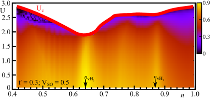
Figure S5: Relative intensity of the ferromagnetic fluctuations in the transversal susceptibility as a function of interaction strength $U$ and filling $n$. The red line indicates the critical interaction strength $U_{c}$. The corresponding plot for the longitudinal susceptibility is shown in Fig. 2 of the main text.

In Fig. S4 we present plots of the longitudinal and transversal RPA spin susceptibility for three different fillings and $U=2.2$. Similar to Fig. 1 in the main text, we observe strong ferromagnetic fluctuations for $n=0.83$ in the longitudinal susceptibility however, with lower intensity. Overall the ${\bf q}$ space structure of the spin fluctuations is quite similar to Fig. 1 in the main text.

In Fig. S5 we show the relative strength of the ferromagnetic fluctuations in the transversal susceptibility as a function of $U$ and filling $n$. In contrast to the longitudinal susceptibility shown in Fig. 2 in the main text, dominant ferromagnetic fluctuations only exist in very narrow regions around the two van Hove fillings $n_{vH_{1}}$ and $n_{vH_{2}}$.

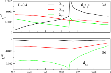
Figure S6: Filling dependence of the intra and inter FS pairing strengths for (a) the $d_{x^{2}-y^{2}}$-wave and (b) the $d_{xy}$-wave pairing symmetry. The corresponding plot for the $f$-wave channel is shown in Fig. 3(c) of the main text.

IV V.   Additional Plots of the pairing strength

In Figs. S6(a)-S6(b) we present the filling dependence of the intra FS ($\lambda^{11}_{i}$ and $\lambda^{22}_{i}$) and the inter FS ($\lambda^{12}_{i}$) pairing strengths for the $d_{x^{2}-y^{2}}$-wave and $d_{xy}$-wave pairing symmetry. We observe that the $d_{x^{2}-y^{2}}$-wave instability is due to scattering within the Fermi sheet FS₁. The case of $d_{xy}$-wave channel is interesting: We find that both inter and intra FS pairing strengths are negative (repulsive), similar to the single FS case ($V_{\textrm{so}}=0$) where $d_{xy}$-wave superconductivity is absent Rømer et al. (2015). However, in a two-band superconductor with two FSs, as for $V_{\textrm{so}}\neq 0$, large negative inter FS interactions (green line) can drive pairing instabilites Dolgov et al. (2009); Dolgov and Golubov (2008). In the present case this occurs for both the $d_{xy}$-wave channel [Fig. S6(b)] and the $p$-wave channel (not shown).

References

- Chiu et al. (2016) C.-K. Chiu, J. C. Y. Teo, A. P. Schnyder, and S. Ryu, Rev. Mod. Phys. 88, 035005 (2016), URL https://link.aps.org/doi/10.1103/RevModPhys.88.035005.
- Hasan and Kane (2010) M. Z. Hasan and C. L. Kane, Rev. Mod. Phys. 82, 3045 (2010).
- Qi and Zhang (2011) X.-L. Qi and S.-C. Zhang, Rev. Mod. Phys. 83, 1057 (2011).
- Schnyder et al. (2008) A. P. Schnyder, S. Ryu, A. Furusaki, and A. W. W. Ludwig, Phys. Rev. B 78, 195125 (2008).
- Schnyder and Brydon (2015) A. P. Schnyder and P. M. R. Brydon, Journal of Physics: Condensed Matter 27, 243201 (2015), URL http://stacks.iop.org/0953-8984/27/i=24/a=243201.
- Sato and Ando (2016) M. Sato and Y. Ando, ArXiv e-prints (2016), eprint 1608.03395.
- Read and Green (2000) N. Read and D. Green, Phys. Rev. B 61, 10267 (2000), URL https://link.aps.org/doi/10.1103/PhysRevB.61.10267.
- Kallin and Berlinsky (2016) C. Kallin and J. Berlinsky, Reports on Progress in Physics 79, 054502 (2016), URL http://stacks.iop.org/0034-4885/79/i=5/a=054502.
- Maeno et al. (2012) Y. Maeno, S. Kittaka, T. Nomura, S. Yonezawa, and K. Ishida, Journal of the Physical Society of Japan 81, 011009 (2012), eprint http://dx.doi.org/10.1143/JPSJ.81.011009, URL http://dx.doi.org/10.1143/JPSJ.81.011009.
- Smidman et al. (2017) M. Smidman, M. B. Salamon, H. Q. Yuan, and D. F. Agterberg, Reports on Progress in Physics 80, 036501 (2017), URL http://stacks.iop.org/0034-4885/80/i=3/a=036501.
- Fu and Kane (2008) L. Fu and C. L. Kane, Phys. Rev. Lett. 100, 096407 (2008), URL https://link.aps.org/doi/10.1103/PhysRevLett.100.096407.
- Yanase and Sigrist (2007) Y. Yanase and M. Sigrist, Journal of the Physical Society of Japan 76, 043712 (2007), URL http://dx.doi.org/10.1143/JPSJ.76.043712.
- Yanase and Sigrist (2008) Y. Yanase and M. Sigrist, Journal of the Physical Society of Japan 77, 124711 (2008), eprint http://dx.doi.org/10.1143/JPSJ.77.124711, URL http://dx.doi.org/10.1143/JPSJ.77.124711.
- Yokoyama et al. (2007) T. Yokoyama, S. Onari, and Y. Tanaka, Phys. Rev. B 75, 172511 (2007), URL http://link.aps.org/doi/10.1103/PhysRevB.75.172511.
- Hor et al. (2010) Y. S. Hor, A. J. Williams, J. G. Checkelsky, P. Roushan, J. Seo, Q. Xu, H. W. Zandbergen, A. Yazdani, N. P. Ong, and R. J. Cava, Phys. Rev. Lett. 104, 057001 (2010), URL https://link.aps.org/doi/10.1103/PhysRevLett.104.057001.
- Sasaki et al. (2011) S. Sasaki, M. Kriener, K. Segawa, K. Yada, Y. Tanaka, M. Sato, and Y. Ando, Phys. Rev. Lett. 107, 217001 (2011), URL https://link.aps.org/doi/10.1103/PhysRevLett.107.217001.
- Levy et al. (2013) N. Levy, T. Zhang, J. Ha, F. Sharifi, A. A. Talin, Y. Kuk, and J. A. Stroscio, Phys. Rev. Lett. 110, 117001 (2013), URL https://link.aps.org/doi/10.1103/PhysRevLett.110.117001.
- Brydon et al. (2014) P. M. R. Brydon, S. Das Sarma, H.-Y. Hui, and J. D. Sau, Phys. Rev. B 90, 184512 (2014), URL https://link.aps.org/doi/10.1103/PhysRevB.90.184512.
- Chakhalian et al. (2007) J. Chakhalian, J. W. Freeland, H.-U. Habermeier, G. Cristiani, G. Khaliullin, M. van Veenendaal, and B. Keimer, Science 318, 1114 (2007), ISSN 0036-8075, eprint http://science.sciencemag.org/content/318/5853/1114.full.pdf, URL http://science.sciencemag.org/content/318/5853/1114.
- Reyren et al. (2007) N. Reyren, S. Thiel, A. D. Caviglia, L. F. Kourkoutis, G. Hammerl, C. Richter, C. W. Schneider, T. Kopp, A.-S. Rüetschi, D. Jaccard, et al., Science 317, 1196 (2007), ISSN 0036-8075, eprint http://science.sciencemag.org/content/317/5842/1196.full.pdf, URL http://science.sciencemag.org/content/317/5842/1196.
- Mizukami et al. (2011) Y. Mizukami, H. Shishido, T. Shibauchi, M. Shimozawa, S. Yasumoto, D. Watanabe, M. Yamashita, H. Ikeda, T. Terashima, H. Kontani, et al., Nat Phys 7, 849 (2011), URL http://dx.doi.org/10.1038/nphys2112.
- Shimozawa et al. (2014) M. Shimozawa, S. K. Goh, R. Endo, R. Kobayashi, T. Watashige, Y. Mizukami, H. Ikeda, H. Shishido, Y. Yanase, T. Terashima, et al., Phys. Rev. Lett. 112, 156404 (2014), URL http://link.aps.org/doi/10.1103/PhysRevLett.112.156404.
- Caviglia et al. (2008) A. D. Caviglia, S. Gariglio, N. Reyren, D. Jaccard, T. Schneider, M. Gabay, S. Thiel, G. Hammerl, J. Mannhart, and J. M. Triscone, Nature 456, 624 (2008), URL http://dx.doi.org/10.1038/nature07576.
- Stock et al. (2008) C. Stock, C. Broholm, J. Hudis, H. J. Kang, and C. Petrovic, Phys. Rev. Lett. 100, 087001 (2008), URL https://link.aps.org/doi/10.1103/PhysRevLett.100.087001.
- Rømer et al. (2015) A. T. Rømer, A. Kreisel, I. Eremin, M. A. Malakhov, T. A. Maier, P. J. Hirschfeld, and B. M. Andersen, Phys. Rev. B 92, 104505 (2015), URL http://link.aps.org/doi/10.1103/PhysRevB.92.104505.
- Scalapino et al. (1986) D. J. Scalapino, E. Loh, and J. E. Hirsch, Phys. Rev. B 34, 8190 (1986), URL https://link.aps.org/doi/10.1103/PhysRevB.34.8190.
- Hlubina (1999) R. Hlubina, Phys. Rev. B 59, 9600 (1999), URL https://link.aps.org/doi/10.1103/PhysRevB.59.9600.
- Meza and Riera (2014) G. A. Meza and J. A. Riera, Phys. Rev. B 90, 085107 (2014), URL https://link.aps.org/doi/10.1103/PhysRevB.90.085107.
- (29) See Supplemental Material for a derivation of Eqs. (4), (5), and (6) and additional plots of the spin susceptibility and the pairing strengths.
- foo (a) Since we focus on weak coupling, it is sufficient to consider only the static pairing interaction.
- Frigeri et al. (2006) P. A. Frigeri, D. F. Agterberg, I. Milat, and M. Sigrist, The European Physical Journal B - Condensed Matter and Complex Systems 54, 435 (2006), ISSN 1434-6036, URL http://dx.doi.org/10.1140/epjb/e2007-00019-5.
- Dolgov and Golubov (2008) O. V. Dolgov and A. A. Golubov, Phys. Rev. B 77, 214526 (2008), URL https://link.aps.org/doi/10.1103/PhysRevB.77.214526.
- Dolgov et al. (2009) O. V. Dolgov, I. I. Mazin, D. Parker, and A. A. Golubov, Phys. Rev. B 79, 060502 (2009), URL https://link.aps.org/doi/10.1103/PhysRevB.79.060502.
- Hirschfeld et al. (2011) P. J. Hirschfeld, M. M. Korshunov, and I. I. Mazin, Reports on Progress in Physics 74, 124508 (2011), URL http://stacks.iop.org/0034-4885/74/i=12/a=124508.
- foo (b) The weak coupling approach neglects retardations and restricts the momenta to the Fermi surfaces. This makes the calculation of , Eq. (6), overly sensitive to the density of states, which is large very close to the van Hove fillings. For this reason the weak coupling approach should be considered with care close to .
- Frigeri et al. (2004) P. A. Frigeri, D. F. Agterberg, A. Koga, and M. Sigrist, Phys. Rev. Lett. 92, 097001 (2004), URL https://link.aps.org/doi/10.1103/PhysRevLett.92.097001.
- Yanase et al. (2003) Y. Yanase, T. Jujo, T. Nomura, H. Ikeda, T. Hotta, and K. Yamada, Physics Reports 387, 1 (2003), ISSN 0370-1573, URL http://www.sciencedirect.com/science/article/pii/S0370157303003235.
- Metzner et al. (2012) W. Metzner, M. Salmhofer, C. Honerkamp, V. Meden, and K. Schönhammer, Rev. Mod. Phys. 84, 299 (2012), URL https://link.aps.org/doi/10.1103/RevModPhys.84.299.
- foo (c) In Ref. Michaeli and Fu (2012) it was shown that spin-orbit locking protects three-dimensional odd-parity superconductors against disorder, due to an emergent chiral symmetry. A similar protection mechanism is expected to occur in the Rashba-Hubbard model. A detailed study of this is left for further investigations.
- Michaeli and Fu (2012) K. Michaeli and L. Fu, Phys. Rev. Lett. 109, 187003 (2012), URL https://link.aps.org/doi/10.1103/PhysRevLett.109.187003.
Supplemental material: