A Strange Metal from Gutzwiller correlations in infinite dimensions II: Transverse Transport, Optical Response and Rise of Two Relaxation Rates

Abstract

Using two approaches to strongly correlated systems, the extremely correlated Fermi liquid theory and the dynamical mean field theory, we compute the transverse transport coefficients, namely the Hall constants $R_{H}$ and Hall angles $\theta_{H}$, and the longitudinal and transverse optical response of the $U=\infty$ Hubbard model in the limit of infinite dimensions. We focus on two successive low-temperature regimes, the Gutzwiller correlated Fermi liquid (GCFL) and the Gutzwiller correlated strange metal (GCSM). We find that the Hall angle $\cot\theta_{H}$ is proportional to $T^{2}$ in the GCFL regime, while on warming into the GCSM regime it first passes through a downward bend and then continues as $T^{2}$. Equivalently, $R_{H}$ is weakly temperature dependent in the GCFL regime, but becomes strongly temperature dependent in the GCSM regime. Drude peaks are found for both the longitudinal optical conductivity $\sigma_{xx}(\omega)$ and the optical Hall angles $\tan\theta_{H}(\omega)$ below certain characteristic energy scales. By comparing the relaxation rates extracted from fitting to the Drude formula, we find that in the GCFL regime there is a single relaxation rate controlling both longitudinal and transverse transport, while in the GCSM regime two different relaxation rates emerge. We trace the origin of this behavior to the dynamical particle-hole asymmetry of the Dyson self-energy, arguably a generic feature of doped Mott insulators.

I Introduction

In a recent study Ding et al. (2017) we have presented results for the longitudinal resistivity and low-temperature thermodynamics of the Hubbard model (with the repulsion parameter $U=\infty$) in the infinite dimensional limit. In this limit, we can obtain the complete single-particle Green’s functions using two methods: the dynamic mean field theory (DMFT) Vollhardt1989 ; Georges1996 ; Deng et al. (2012); Xu et al. (2013), and the extremely correlated Fermi liquid (ECFL) theoryShastry and Perepelitsky (2016); Shastry (2011), with some overlapping results and comparisons in Ref. [Rok, ]. These studies capture the non-perturbative local Gutzwiller correlation effects on the longitudinal resistivity $\rho_{xx}$ quantitativelyDeng et al. (2012); Xu et al. (2013); Shastry and Perepelitsky (2016). A recent study by our group addresses the physically relevant case of two dimensionsShastry-Mai , with important results for many variables discussed here.

The present work extends the study of Ref. [Ding et al., 2017], using the ECFL scheme of Ref. [Shastry and Perepelitsky, 2016], to the case of the Hall conductivity $\sigma_{xy}$ and the finite frequency (i.e. optical) conductivities. One goal is to further test ECFL with the exact DMFT results for these quantities which are more challenging to calculate. More importantly, however, by combining the various calculated conductivities we are able to uncover the emergence of two different transport relaxation times. In cuprate superconductors, various authors Chien et al. (1991); Anderson (1991); Ando ; Boebinger ; NCCO have commented on the different temperature ($T$) dependence of the transport properties in the normal phase. The cotangent Hall angles, defined as the ratio of the longitudinal conductivity $\sigma_{xx}$ and the Hall conductivity, $\cot(\theta_{H})=\sigma_{xx}/\sigma_{xy}$, is close to quadratic as in conventional metals. Meanwhile, the longitudinal resistivity has unusual linear temperature dependence Ando et al. (2004). Understanding the ubiquitous $T^{2}$ behavior of $\cot(\theta_{H})$ in spite of the unconventional temperature dependence of the longitudinal resistivity is therefore quite important.

In Ref. [Ding et al., 2017] we found that at the lowest temperatures the system is a Gutzwiller-correlated Fermi liquid (GCFL) with $\rho_{xx}\propto T^{2}$. Upon warming one finds a regime with linear temperature dependence of the resistivity $\rho_{xx}$Ding et al. (2017), which is reminiscent of the strange metal regime in the cuprate phase diagrams Ando et al. (2004). It is termed the Gutzwiller-correlated strange metal (GCSM) regimeDing et al. (2017). Previous studiesDeng et al. (2012); Xu et al. (2013) established the GCFL and GCSM regimes using the longitudinal resistivity. Here we focus instead on the Hall constants $R_{H}=\sigma_{xy}/\sigma_{xx}^{2}$ and the Hall anglesXu et al. (2013), as well as on the optical conductivityDeng et al. (2012) and optical Hall angles. In the GCFL regime, the primary excitations are coherent quasiparticles that survive the Gutzwiller correlation, and there is a single transport relaxation time, as one would expect for a conventional Fermi liquid. Upon warming up into the GCSM regime, the longitudinal and transverse optical scattering rates become different. It appears that the existence of two separate scattering times is a generic characteristic of the GCSM regime.

This work is organized as follows. First we summarize the Kubo formulas used to calculate the transport coefficients in Sec. (II). We then revisit in Sec. (III) the familiar Boltzmann transport theory from which two separate relaxation times can be naturally derived. The results for the $dc$ transport properties are presented in Sec. (IV) and those of optical conductivities in Sec. (V). In Sec. (VI) we interpret the two scattering times found in the GCSM regime through the particle-hole asymmetry of dynamical properties (spectral function) of the system. In conclusion we discuss the implication of this work for strongly correlated matter.

II Kubo formulas

The transport properties of correlated materials can be easily evaluated in the limit of infinite dimensions because the vertex corrections are absentKhurana (1990). For dimensions $d>3$, the longitudinal conductivity $\sigma_{xx}$ is straightforwardly generalized as the electric field remains a $d$-dimensional vector. The generalization is less clear for the transverse conductivity and Hall constants, because the magnetic field is no longer a vector but rather a rank-2 tensor defined through the electromagnetic tensor. Nevertheless, $\sigma_{xy}$ can still be defined through suitable current-current correlation functions.

The input to the transport calculation is the single-particle Green’s function $G(\omega,\bm{k})$, calculated in the following within either ECFL or DMFT. The Kubo formulas can be written as Pruschke et al. (1993); Voruganti et al. (1992)

$$\sigma_{xx}=2\pi q_{e}^{2}\sum_{k}\Phi_{k}^{xx}\int d\omega(-\frac{\partial f(\omega)}{\partial\omega})\rho^{2}_{G}(\omega,\bm{k}),$$ (1)

$$\sigma_{xy}/B=\frac{4\pi^{2}q_{e}^{3}}{3}\sum_{k}\Phi_{k}^{xy}\int d\omega(-\frac{\partial f(\omega)}{\partial\omega})\rho^{3}_{G}(\omega,\bm{k}),$$ (2)

where $\rho_{G}(\omega,\bm{k})=-\mathcal{I}mG(\omega,\bm{k})/\pi$ is the single-particle spectral function and $q_{e}=-|e|$ is the electron charge. $\Phi_{k}^{xx}=(\epsilon_{k}^{x})^{2}$ and $\Phi_{k}^{xy}=(\epsilon_{k}^{y})^{2}\epsilon_{k}^{xx}-\epsilon_{k}^{y}\epsilon_{k}^{x}\epsilon_{k}^{xy}$ are called transport functions, with $\epsilon^{\alpha}_{k}=\partial\epsilon_{k}/\partial k_{\alpha}$ and $\epsilon^{\alpha\beta}_{k}=\partial^{2}\epsilon_{k}/\partial k_{\alpha}\partial k_{\beta}$, $\epsilon_{k}$ being the energy dispersion. We set $\hbar$ to 1.

It is more convenient to convert the multi-dimensional $k$-sums into energy integrals:

$$\sigma_{xx}=\sigma_{0}2\pi D\int d\epsilon\frac{\Phi^{xx}(\epsilon)}{\Phi^{xx}(0)}\int d\omega(-\frac{\partial f(\omega)}{\partial\omega})\rho^{2}_{G}(\omega,\epsilon),$$ (3)

$$\sigma_{xy}/B=\sigma_{0}\frac{4\pi^{2}Dq_{e}}{3}\int d\epsilon\frac{\Phi^{xy}(\epsilon)}{\Phi^{xx}(0)}\int d\omega(-\frac{\partial f(\omega)}{\partial\omega})\rho^{3}_{G}(\omega,\epsilon),$$ (4)

where $\Phi^{xx(xy)}(\epsilon)=\sum_{\bm{k}}\Phi_{\bm{k}}^{xx(xy)}\delta(\epsilon-\epsilon_{\bm{k}})$, $\sigma_{0}=q_{e}^{2}\Phi^{xx}(0)/D$ is the Ioffe-Regel-Mott conductivity, $D$ is half-bandwidth, and $\rho_{G}(\omega,\epsilon)=\rho_{G}(\omega,\bm{k})$ such that $\epsilon=\epsilon_{k}$. In $d$ dimensions the transport functions on the Bethe lattice are Arsenault and Tremblay (2013)

$$\Phi^{xx}(\epsilon)=\frac{1}{3d}(D^{2}-\epsilon^{2})\rho_{0}(\epsilon),$$ (5)

$$\Phi^{xy}(\epsilon)=-\frac{1}{3d(d-1)}\epsilon(D^{2}-\epsilon^{2})\rho_{0}(\epsilon),$$ (6)

where $\rho_{0}(\epsilon)=\frac{2}{\pi D^{2}}\sqrt{D^{2}-\epsilon^{2}}\Theta(D-|\epsilon|)$ is the non-interacting density of states on the Bethe lattice and $D$ is the half bandwidth. Even though the transport function results indicate that $\sigma$ vanishes as $d\rightarrow\infty$, we can redefine the conductivities in this limit as the sum of all components: $\sigma_{L}=\sum_{\alpha}\sigma_{\alpha\alpha}$, $\sigma_{T}=\sum_{\alpha\neq\beta}\text{Sgn}[\alpha-\beta]\sigma_{\alpha\beta}$ with $\alpha(\beta)=1,2,\dots,d$. More importantly, the $d$-dependence directly drops out when we compute the Hall constant $R_{H}=\sigma_{xy}/\sigma_{xx}^{2}$. For the rest of this work, we shall re-define $\sigma_{xx}$ and $\sigma_{xy}$ via $\sigma_{L}$ and $\sigma_{T}$ considering that all components of $\sigma_{L(T)}$ are equal so that both the $d$-factor and the constant factor drop out from the transport functions:

$$\sigma_{xx}=3\sigma_{L},\qquad\Phi^{xx}(\epsilon)=(D^{2}-\epsilon^{2})\rho_{0}(\epsilon),$$ (7)

$$\sigma_{xy}=3\sigma_{T},\qquad\Phi^{xy}(\epsilon)=-\epsilon(D^{2}-\epsilon^{2})\rho_{0}(\epsilon).$$ (8)

III Two-relaxation-time behavior in the Boltzmann theory

In Boltzmann theory, the transport properties can be obtained by solving for the distribution function in the presence of external fields from the Boltzmann equationZiman (1960):

$$\frac{\partial\,\delta\!f}{\partial t}-\frac{q_{e}}{\hbar c}\bm{v}\times\bm{B}\cdot\frac{\partial\,\delta\!f}{\partial\bm{k}}+\bm{v}\cdot q_{e}\bm{E}(t)\left(-\frac{\partial f^{0}}{\partial\epsilon}\right)=\hat{L}\,\delta\!f,$$ (9)

where $f$ is the full distribution function that needs to be solved, $f^{0}$ is the Fermi-Dirac distribution function, $\delta\!f=f-f^{0}$, and $\hat{L}\delta\!f$ represents the linearized collision integrals.

In the regime of linear response, we expand $\delta\!f^{E,B}$ in powers of the external fields to second order as

$$\delta\!f^{E,B}=\delta\!f^{E,0}+B\delta\!f^{E,1},$$ (10)

where $\delta\!f^{E,0}$ is the solution in the absence of magnetic fields, and both $\delta\!f^{E,0}$ and $\delta\!f^{E,1}$ are linear in $E$. In the relaxation-time-approximation (RTA)Feng and Jin (2005) we replace the collision integrals as $\hat{L}_{\bm{k}}\delta\!f\rightarrow-\delta\!f/\tau$ where $\tau$ is assumed to be $\bm{k}$-independent. However, $\hat{L}\delta\!f^{E,0}$ and $\hat{L}\delta\!f^{E,1}$ are in principle governed by different relaxation times, as pointed out by Anderson Chien et al. (1991); Anderson (1991). Writing

$$\hat{L}\delta\!f^{E,0}\rightarrow-\frac{\delta\!f^{E,0}}{\tau_{tr}},\qquad\hat{L}\delta\!f^{E,1}\rightarrow-\frac{\delta\!f^{E,1}}{\tau_{H}},$$ (11)

we obtain

$$\sigma_{xx}(\omega)=\frac{\omega_{p}^{2}}{4\pi}\frac{\tau_{tr}}{1-i\omega\tau_{tr}},$$ (12)

$$\sigma_{xy}(\omega)/B=\frac{\omega_{p}^{2}\omega_{c}/B}{4\pi^{2}}\frac{\tau_{H}}{1-i\omega\tau_{H}}\frac{\tau_{tr}}{1-i\omega\tau_{tr}},$$ (13)

where

$$\frac{\omega_{p}^{2}}{4\pi}=\int\frac{d^{d}k}{(2\pi)^{d}}2q_{e}^{2}v_{x}^{2}(-\partial_{\epsilon}f^{0}),$$ (14)

$$\frac{\omega_{c}}{B}=\omega_{p}^{-2}\int\frac{d^{d}k}{(2\pi)^{d}}2q_{e}^{3}(v_{x}^{2}\partial_{k_{y}}v_{y}-v_{x}v_{y}\partial_{k_{x}}v_{y})\partial_{\epsilon}f^{0},$$ (15)

$v_{a}=\partial_{k_{a}}\epsilon(\bm{k})$ is the velocity in direction $a$, $\epsilon(\bm{k})$ is energy dispersion of the electrons and ${\bf B}=\hat{z}B$. Then the Hall angle is

$$\tan\theta_{H}(\omega)=\frac{\omega_{c}}{\pi}\frac{\tau_{H}}{1-i\omega\tau_{H}}.$$ (16)

Therefore, the optical conductivities can be cast in the Boltzmann-RTA form as

$$\frac{\sigma_{xx}(0)}{\mathcal{R}e[\sigma_{xx}(\omega)]} =1+\omega^{2}\tau_{tr}^{2},$$ (17)

$$\frac{\sigma_{xy}(0)/B}{\mathcal{R}e[\sigma_{xy}(\omega)]/B} =1+\omega^{2}(\tau_{tr}^{2}+\tau_{H}^{2})+\tau_{tr}^{2}\tau_{H}^{2}\omega^{4},$$ (18)

$$\frac{\theta_{H}(0)}{\mathcal{R}e[\theta_{H}(\omega)]} =1+\omega^{2}\tau_{H}^{2}.$$ (19)

The $dc$ and $ac$ transport coefficients of a microscopic theory do not necessarily take the form of the Boltzmann RTA theory. In the rest of this work, we study both the $dc$ and the real part of the $ac$ transport coefficients, and consider them as

$$\Re e[\sigma_{xx}(\omega)]=\frac{\sigma_{xx}(0)}{1+\tau^{2}_{tr}\omega^{2}+\mathcal{O}(\omega^{4})},$$ (20)

$$\Re e[\tan\theta_{H}(\omega)/B]=\frac{\tan\theta_{H}(0)/B}{1+\tau_{H}^{2}\omega^{2}+\mathcal{O}(\omega^{4})}.$$ (21)

The relaxation times $\tau_{tr}$ and $\tau_{H}$ are extracted from the low frequency part of $\Re e[\sigma_{xx}(\omega)]$ and $\Re e[\tan\theta_{H}(\omega)/B]$ by fitting to the above expressions. Although computing $\mathcal{R}e[\theta_{H}(\omega)]$ requires both real and imaginary parts of the optical conductivities, we can make the approximation $\mathcal{R}e[\theta_{H}(\omega)]\simeq\mathcal{R}e[\sigma_{xy}(\omega)]/\mathcal{R}e[\sigma_{xx}(\omega)]$ when $\omega$ of concern is small. We expect $\tau_{tr}$ and $\tau_{H}$ to have similar temperature and density dependence as $\sigma_{xx}(0)$ and $\tan\theta_{H}(0)/B$.

IV $dc$ Transport

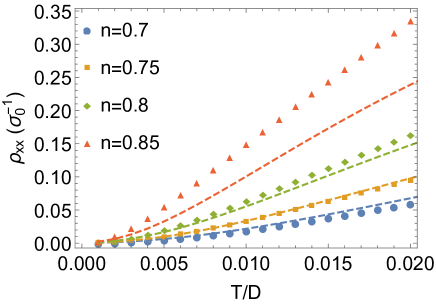
Figure 1: Temperature dependence of the $dc$ resistivity $\rho_{xx}$ of the $U=\infty$ Hubbard model from DMFT (dashed lines) and ECFL (solid symbols) for a range of electron densities $n$. The horizontal axis corresponds to absolute temperatures.

We now use the Kubo formulas to compute the transport coefficients within the ECFL and DMFT approaches. We plot the ECFL results as solid symbols and the DMFT results as dashed lines using the same color for each density unless specified otherwise. As we shall demonstrate, the agreement between the DMFT and ECFL results follows the same qualitative trend for all quantities considered: it is better at lower temperatures, lower frequencies, and at lower density (higher hole doping).

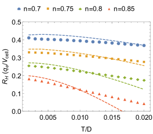
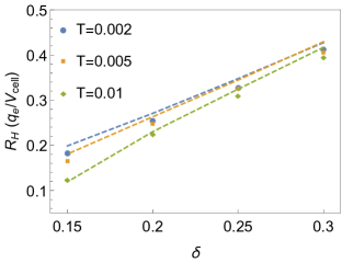
Figure 2: Temperature dependence of the Hall constants $R_{H}$ (2) and $R_{H}$ at $T=0.002D,0.005D,0.01D$ as functions of the hole density $\delta=1-n$ (2) for both DMFT (dashed lines) and ECFL (solid symbols). $R_{H}$ is weakly $T$-dependent below $T_{FL}$ and develops stronger $T$-dependence in the GCSM regime. $R_{H}$ varies roughly linearly on $\delta$ at all three temperatures shown in (2).

We identify the GCFL and GCSM regimes, as well as the cross-over scale $T_{FL}$ separating them, from the T dependence of the longitudinal resistivity $\rho_{xx}$, shown in Fig. (1). We identify the Fermi liquid temperature $T_{FL}$ using the resistivity, rather than the more conventional thermodynamic measures, such as heat capacity. The latter variables do actually give rather similar values, but the resistivity seems most appropriate for this study. Our definition is that up to and below $T_{FL}$, the resistivity $\rho_{xx}\sim T^{2}$, while above $T_{FL}$, $\rho_{xx}$ displays a more complex set of $T$ dependence as outlined in Ref. [Ding et al., 2017]. The Fermi liquid temperature has been quantitatively estimated in Ref. [Shastry and Perepelitsky, 2016]:

$$T_{FL}\simeq 0.05\times D\delta^{\alpha},$$ (22)

where $\delta$ is the hole density $\delta=1-n$. The exponent $\alpha\sim 1.39$ within DMFT Rok ; this is the value we will use below. $\alpha$ is somewhat greater for ECFL within the scheme used in Ref. [Shastry and Perepelitsky, 2016] and hence $T_{FL}$ given by DMFT is slightly higher than that by ECFL, as can also be seen in Fig. (1). Consequently as $n$ increases, the the ECFL curves for $\rho_{xx}$ lie above those from DMFT.

IV.1 Hall constant

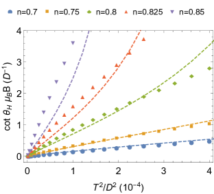
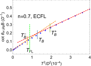
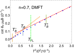
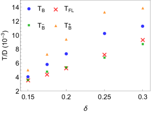
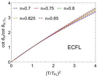
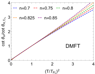
Figure 3: Temperature dependence of the cotangent Hall angle $\cot\theta_{H}B$ of both ECFL (symbols) and DMFT (dashed lines) shown as a function of $T^{2}$ (3). The Hall angles $\cot\theta_{H}B\propto T^{2}$ in the GCFL regime, passes through a slight downward bend (i.e., a kink), and continues as $T^{2}$ within the temperature range studied. The downward bending regime is characterized by its onset $T_{B}^{-}$, the crossing of the two different $T^{2}$ lines $T_{B}$, and its ending $T_{B}^{+}$. We illustrate the kink and the determination of $T_{B}$, $T_{B}^{-}$ and $T_{B}^{+}$ at $n=0.7$ for both ECFL (3) and DMFT (3). $T_{B}$, $T_{B}^{-}$ and $T_{B}^{+}$ obtained from the ECFL are shown as a function of $\delta$ in (3). We plot $\frac{\cot\theta_{H}}{\cot\theta_{H}(T=T_{FL})}$ as functions of $(T/T_{FL})^{2}$ for ECFL (3) and DMFT (3) to show the systematic evolution of the kinks when the density varies.

In Fig. (2), we show $R_{H}$ as a function of temperature at different densities for low temperatures $T<0.02D$ (2), and as a function of the hole density $\delta=(1-n)$ at $T=0.002D,0.005D,0.01D$ (2). The Hall constant is weakly temperature-dependent for $T\ll T_{FL}$, but it starts to decrease on warming, as seen in Fig. (2).

As a function of density $\delta$ the Hall constants from the two theories agree quite well, and are roughly linear with $\delta$. The extrapolation to $\delta\to 0$ is uncertain from the present data. One might be tempted to speculate that it vanishes, since the lattice density of states is particle-hole symmetric. This question deserves further study with different densities of states that break the particle-hole symmetry.

IV.2 Cotangent of the Hall angle

The theoretical results for cotangent of the Hall angle $(\cot\theta_{H})B=(\sigma_{xx}/\sigma_{xy})B$ are shown as a function of $T^{2}$ in Fig. (3). We see that in DMFT as well as ECFL, the $\cot(\theta_{H})$ is linear in $T^{2}$ on both sides of a bend (or kink) temperature, which increases with increasing hole density $\delta$. However this kink is weaker in DMFT than in ECFL. This bending was already noted in Fig.  (5.a) of Ref. (Shastry-Mai, ), within the 2-d ECFL theory. We may thus infer that $\cot(\theta_{H})$ goes as $Q_{FL}T^{2}$ in the Fermi liquid regime, passes through a slight downward bend, and continues as $Q_{SM}T^{2}$ in the strange metal regimes, such that $Q_{FL}>Q_{SM}$. The difference, $A_{FL}-A_{SM}$, becomes smaller as $\delta$ decreases.

In order to characterize this kink more precisely, we define the downward bending regime by its onset temperature $T_{B}^{-}$, the crossing temperature of the two different $T^{2}$ lines $T_{B}$, and its ending temperature $T_{B}^{+}$. The temperatures $T_{B}^{-(+)}$ are determined by 5% deviation from the $T^{2}$-fitting well below (above) $T_{FL}$, and $T_{B}$ is well defined as the crossing point of the two $T^{2}$-fittings. We illustrate the kink and the determination of $T_{B}$, $T_{B}^{-}$ and $T_{B}^{+}$ at $n=0.7$ for both ECFL in Fig. (3) and DMFT in Fig. (3). In Fig. (3), we show $T_{B},\ T_{B}^{-},\ T_{B}^{+}$ and $T_{FL}$ obtained from ECFL as functions of $\delta$. We see that $T_{B}^{-}$ is identical to $T_{FL}$, while $T_{B}$ and $T_{B}^{+}$ are $T_{FL}$ plus some constants with weak $\delta$-dependence. We plot $\frac{\cot\theta_{H}}{\cot\theta_{H}(T=T_{FL})}$ as functions of $(T/T_{FL})^{2}$ for ECFL in Fig. (3) and DMFT in Fig. (3) to show the systematic evolution of the kinks when the density is varied.

IV.3 Kink in cotangent of the Hall angle

There has been much interest in the quadratic $T$ dependence of $\cot(\theta_{H})$ in the literature Chien et al. (1991); Anderson (1991). It is intriguing that a kink in the plot of $\cot(\theta_{H})$ versus $T^{2}$ curves is seen in almost all experiments, although it appears to not have been commented on earlier. Such bending is clearly seen in experimental data Fig. (2) of Ref. [Chien et al., 1991], Fig. (4) of Ref. [Hwang1994, ] and Fig. (3.c) of Ref. [Ando2004, ].

From Fig. (3.c) of Ref. [Ando2004, ] we estimate $T_{B}\simeq 100\ K,80\ K,70\ K$ for LSCO at $\delta=0.21,\ 0.17,\ 0.14$ respectively. These are comparable with the ECFL results $T_{B}=70\ K,\ 60\ K,\ 40\ K$ at $\delta=0.2,\ 0.175,\ 0.15$, if we set $D=10^{4}\ K$. The trend of $T_{B}$ and the prefactor difference $A_{FL}-A_{SM}$ also agrees with what we find, i.e., both $T_{B}$ and $A_{FL}-A_{SM}$ decrease as $\delta$ is lowered. An increase of $A_{SM}$ at even higher temperatures is also observed in Ref.[Ando2007, ], similar as what we find in Fig. (3) above the GCSM regime.

It is notable that the bending temperatures $T_{B}$ in theory and in experiments are on a similar scale. It is therefore of interest to explore this kink in $\cot(\theta_{H})$ more carefully. From the perspective of the ECFL and DMFT theories, we note that the kink represents one of the basic crossovers discussed in Ref. [Ding et al., 2017], namely from the GCFL to GCSM regimes. It would be interesting to explore this feature more closely in experiments, in particular to see if the theoretically expected correlation between the crossover in $\rho_{xx}$ and $\cot(\theta_{H})$ finds support.

V Optical response

V.1 Optical conductivity and the longitudinal scattering rates $\Gamma_{tr}$

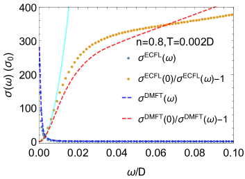
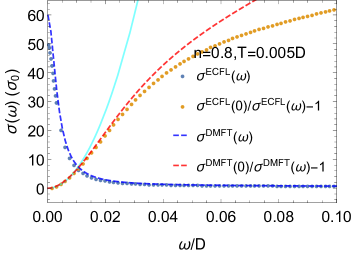
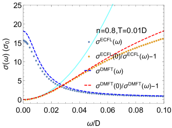
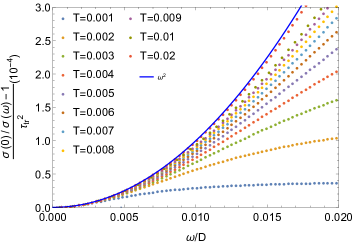
Figure 4: $\sigma_{xx}(\omega)$ and $\sigma(0)/\sigma(\omega)-1$ for $n=0.8$ at $T=0.002D$ (4), $T=0.005D$ (4) and $T=0.01D$ (4) for DMFT (dashed lines) and ECFL (solid symbols). The cyan solid lines are $\omega^{2}$ fitting near $\omega\to 0$. In (4) we normalize $\sigma(0)/\sigma(\omega)-1$ curves computed from ECFL for various temperatures by $\tau_{tr}^{2}$ with $\tau_{tr}$ obtained from the fits at small frequencies to the Drude formula. The solid blue line is a $\omega^{2}$ curve.

In Fig. (4) we show the optical conductivity $\sigma_{xx}(\omega)$ as well as the quantity $\sigma_{xx}(0)/\sigma_{xx}(\omega)-1$, which better presents the approach to the zero frequency limit and is to be compared with the Boltzmann RTA form (Drude formula) in Eq. (17). We display plots obtained from both ECFL (symbols) and DMFT (dashed lines) for fixed $n=0.8$ and for three temperatures to show the generic behavior at $T<T_{FL}$, $T\simeq T_{FL}$ and $T>T_{FL}$: $T=0.002D$ (4), $T=0.005D$ (4) and $T=0.01D$ (4). ECFL results agree well with the exact solution of DMFT within this temperature range.

$\sigma_{xx}(\omega)$ shows a narrow Drude peak below $T_{FL}$ which broadens as $T$ increases and finally takes a form well approximated by a broad Lorentzian at $T=0.01$ D. Correspondingly, $(\sigma_{xx}(0)/\sigma_{xx}(\omega)-1)$ is quadratic in frequency and can be fit to $\tau_{tr}^{2}\omega^{2}$ to extract the relaxation time $\tau_{tr}$. The $\omega^{2}$ regime has a width $\propto\tau^{-1}_{tr}$. The fitting is performed at very small frequencies well within this quadratic regime. At higher frequency, $(\sigma_{xx}(0)/\sigma_{xx}(\omega)-1)$ flattens out and creates a knee-like feature in-between. The flattening tendency decreases as $T$ increases, and $1/\sigma_{xx}(\omega)$ grows monotonically. This knee-like feature thus becomes smoother as $T$ increases and eventually is lost for $T>T_{FL}$. This trend is illustrated in Fig. (4), where we normalize all curves of $(\sigma_{xx}(0)/\sigma_{xx}(\omega)-1)$ by their corresponding $\tau_{tr}^{2}$, while the $\omega^{2}$ curve is shown as a solid blue line. All curves fall onto the $\omega^{2}$ line at small frequencies, and peal off at a frequency which increases as $T$ increases.

These scattering rates are shown as a function of temperature in Fig. (6). The scattering rate $\Gamma$ has a similar temperature dependence as the resistivity, i.e., a quadratic-T regime at low temperatures followed by a linear-T regime at higher temperatures.

V.2 Optical Hall angle and the transverse scattering rates $\Gamma_{H}$

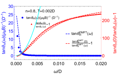
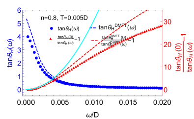
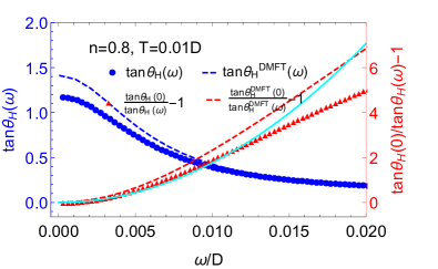
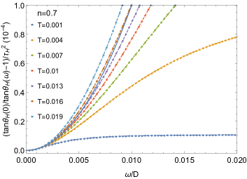
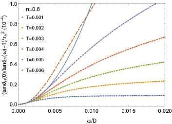
Figure 5: Optical Hall angles $\tan\theta_{H}(\omega)$ (blue) and $\tan\theta_{H}(0)/\tan\theta_{H}(\omega)-1$(red) shown for $n=0.8$, $T=0.002D$ (5), $T=0.005D$ (5) and $T=0.01D$ (5) for DMFT (dashed lines) and ECFL (solid symbols). The cyan solid lines are $\omega^{2}$ fitting near $\omega\to 0$. $[\tan\theta_{H}(0)/\tan\theta_{H}(\omega)-1]/\tau_{H}^{2}$ obtained from ECFL shown for $n=0.7$ (5) and $n=0.8$ (5). Drude peaks are found to be narrow (note the different horizontal axis scale compared to Fig. 3).

In Fig. (5), we show the optical tangent Hall angle $\tan\theta_{H}(\omega)$ and the quantity $\tan\theta_{H}(0)/\tan\theta_{H}(\omega)-1$. We display plots obtained from both ECFL (symbols) and DMFT (dashed lines) for fixed $n=0.8$ and for three temperatures to show the generic behavior at $T<T_{FL}$, $T\simeq T_{FL}$ and $T>T_{FL}$: $T=0.002D$ (5), $T=0.005D$ (5) and $T=0.01D$ (5). The ECFL results agree well with those from DMFT within this temperature range.

Just like $\sigma_{xx}(\omega)$, $\tan\theta_{H}(\omega)$ possesses a narrow Drude peak below $T_{FL}$ that broadens in a similar way with increasing temperature. $(\tan\theta_{H}(0)/\tan\theta_{H}(\omega)-1)$ is quadratic in frequency and we fit $\tau_{H}^{2}\omega^{2}$ to extract the transverse relaxation time $\tau_{H}$. The $\omega^{2}$ regime, however, has a very narrow, weakly $T$-dependent width which is about $0.003\ D$. The relaxation time $\tau_{H}$ is extracted by fitting within this very low frequency range. Above this energy a flattening behavior, similar to that in the optical conductivity, takes place at low temperatures. At higher temperatures and lower hole density, a power-law behavior with an exponent that increases with $T$ gradually replaces the flattening out behavior. Such a tendency is visible in Figs. (5) and (5), where all $(\tan\theta_{H}(0)/\tan\theta_{H}(\omega)-1)$ curves are normalized by their corresponding $\tau_{H}^{2}$.

In Fig. (6) we show $\Gamma_{H}$ (defined as $\Gamma_{H}\equiv\tau_{H}^{-1}$) for various densities and temperatures obtained from the Drude formula fitting. Their $T$-dependence is quadratic for both GCFL and GCSM regimes.

V.3 Emergence of two relaxation times

In Fig. (6), we show $\Gamma_{H}/\Gamma_{tr}$ as a function of temperature. At all densities considered this ratio behaves differently for $T$ below and above $T_{FL}$. Below $T_{FL}$, the ratio $\Gamma_{H}/\Gamma_{tr}\simeq 0.5$ remains essentially constant, and hence the optical transport is dominated by a single scattering rate. Once $T_{FL}$ is crossed, however, $\Gamma_{H}/\Gamma_{tr}$ becomes strongly $T$-dependent. This indicates that there are two relaxation times in the GCSM regime. This is possible since the quasiparticles are no longer well defined for $T>T_{FL}$, and different frequency regimes present in the spectral functions contribute differently to the two relaxation times. In Fig. (6), we plot $\Gamma_{H}/\Gamma_{tr}$ versus the rescaled temperature $T/T_{FL}$ to illustrate the clearly distinct behavior below and above $T_{FL}$.

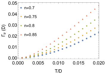
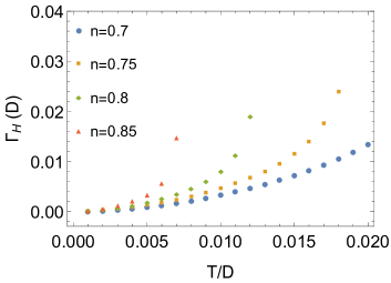
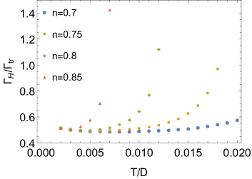
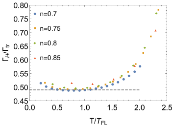
Figure 6: Longitudinal relaxation rate $\Gamma_{tr}$ extracted by fitting $\sigma_{xx}(\omega)$ by the Drude formula (6), transverse relaxation time $\Gamma_{H}$ extracted from $\theta_{H}(\omega)$ (6), their ratio $\Gamma_{H}/\Gamma_{tr}$ as functions of $T$ (6) and as functions of scaled temperature $T/T_{FL}$ (6). All the relaxation rates are extracted from the ECFL optical response results.

VI Analysis

We begin by analyzing the exact formulas for the conductivities $\sigma_{xx},\sigma_{xy}$ of Eqs. (3) and (4), following Ref. [voruganti, ] and [Shastry and Perepelitsky, 2016] within ECFL theory where more analytic insight is available.

It has long been noted that the particle-hole asymmetry of the spectral function is one of the characteristic features of strongly correlated systemsrenner1998 ; anderson2006 ; hanaguri2004 ; casey2008 ; pasupathy2008 ; gweon2011 ; Shastry (2012). The dynamic particle-hole transformation is defined by simultaneously inverting the wave vector and energy in $\rho_{G}(\bm{k},\omega)$ relative to the chemical potential $\bm{\mu}$ as $(\bm{\hat{k}},\omega)\rightarrow-(\bm{\hat{k}},\omega)$, with $\bm{\hat{k}}=\bm{k}-\bm{k}_{F}$Shastry (2012). In the limit of $d\to\infty$, we ignore the $\bm{\hat{k}}$ part of the transformation. Consequently, the dynamic particle-hole asymmetry solely stems from the asymmetry of the self-energy spectral function $\rho_{\Sigma}(\omega,T)=-\mathcal{I}m\Sigma(\omega,T)/\pi$. Instead of analyzing $\rho_{G}$, we can simply focus on $\rho_{\Sigma}$ since

$$\rho_{G} = \frac{\rho_{\Sigma}}{(\omega+\mu-\epsilon-\mathcal{R}e\Sigma)^{2}+\pi^{2}\rho_{\Sigma}^{2}}.$$ (23)

$$= \frac{1}{\pi}\frac{B(\omega,T)}{(A(\omega,T)-\epsilon)^{2}+B^{2}(\omega,T)}$$ (24)

where

$$A(\omega,T)=\omega+\mu-\mathcal{R}e\Sigma(\omega,T),$$ (25)

$$B(\omega,T)=\pi\rho_{\Sigma}(\omega,T)=-\mathcal{I}m\Sigma(\omega,T).$$ (26)

Then we approximate the exact equations (3) and (4) by their asymptotic values at low enough T, following Ref. [Shastry and Perepelitsky, 2016]. The idea is to first integrate over the band energy $\epsilon$ viewing one of the powers of $\rho_{G}$ as a $\delta$ function constraining $\epsilon\to A(\omega,T)$. This gives

$$\sigma_{xx}=\frac{\sigma_{0}D}{\Phi^{xx}[0]}\int d\omega(-f^{\prime})\frac{\Phi^{xx}[A(\omega,T)]}{B(\omega,T)},$$ (27)

$$\sigma_{xy}=\frac{\sigma_{0}Dq_{e}}{\Phi^{xx}[0]}\int d\omega(f^{\prime})\Big{(}\frac{\partial_{\omega}^{2}\Phi^{xy}[A(\omega,T)]}{3}+\frac{\Phi^{xy}[A(\omega,T)]}{2(B(\omega,T))^{2}}\Big{)},$$

(28)

The first term in Eq. (28) turns out to be negligible compared to the second, and hence we will ignore it. Next, we track down the electronic properties that give rise to a second relaxation time using the above asymptotic expressions.

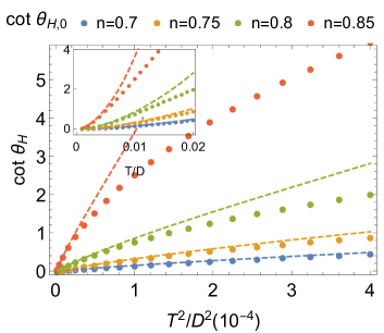
Figure 7: Zeroth order asymptotic cotangent Hall angles $\cot\theta_{H,0}$ plotted as functions of $T^{2}$ (main panel, symbols) compared with the exact results (dashed lines) and as functions of $T$ (inset).

To the lowest order of approximation at low temperatures, we can make the substitution $f^{\prime}(\omega)\to-\delta(\omega)$ in Eq. (27) and (28), which gives

$$\cot\theta_{H,0}/B=\frac{2B(0,T)}{q_{e}A(0,T)}.$$ (29)

We show $\cot\theta_{H,0}$ in Fig. (7). When plotted as a function of $T^{2}$ as shown in the main panel of Fig. (7), $\cot\theta_{H,0}$ (solid symbols) is in good agreement with the exact results (dashed lines) both qualitatively, i.e., showing a kink-like feature, and quantitatively except for relatively high temperatures and densities. However, when it is plotted as a function of $T$ (inset of Fig. (7)), we find that the ”kink” is actually the crossover from a $T^{2}$ behavior to a linear-$T$ behavior and $\cot\theta_{H,0}$ follows the $T$-dependence of $\rho_{xx}$. The lowest order approximation is insufficient to capture and to understand the second $T^{2}$ regime. Therefore, we pursue more accurate asymptotic expressions of Eqs. (27) and (28). Following Ref. [Xu et al., 2013] and [Ding et al., 2017], we do the following small frequency expansion:

$$\begin{split}&\Phi^{xx(xy)}[A(\omega,T)]=\Phi^{xx(xy)}[A_{0}]\\ &+\Phi^{xx(xy)\prime}[A_{0}]A_{1}\ \omega+\dots,\end{split}$$ (30)

$$B(\omega,T)=B_{0}+B_{1}\omega+B_{2}\omega^{2}+\dots,$$ (31)

where $A_{0}$ and $A_{1}$ is given by the expansion

$$A(\omega,T)=A_{0}+A_{1}\omega+\dots,$$ (32)

Recall that $A_{1}=Z^{-1}$, it is therefore large. In order to provide further context to these coefficients $B_{n}$ and to connect with earlier discussions of the self energy, it is useful to recall a useful and suggestive expression for the imaginary self energy exhibiting particle-hole asymmetry at $k_{F}$ at low $\omega$ (e.g. see Eq. (28) in Ref. [Rok, ])

$$-\Im\,m\Sigma(\omega,T)\sim\pi\frac{(\omega^{2}+\pi^{2}T^{2})}{\Omega_{\Sigma}(T)}\left(1-\frac{\omega}{\Delta}\right),$$ (33)

where $\Omega_{\Sigma}$ behaves as $\sim Z^{2}$ in the low-$T$ Fermi liquid regime. The scale $\Delta$ breaks the particle-hole symmetry of the leading term.

The variation of $\Omega_{\Sigma}$ and $\Delta$ in the GCSM regime is illustrated below in Fig. (8). Expanding this expression at low $\omega$ we identify the coefficients $B_{0}=\pi\frac{\pi^{2}T^{2}}{\Omega_{\Sigma}(T)}$, $B_{1}=-\frac{B_{0}}{\Delta}$, $B_{2}=\frac{\pi}{\Omega_{\Sigma}}$, all of which are numerically verified to be valid for all temperatures we study in this work. The negative sign of $B_{1}$ is easily understood.

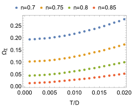
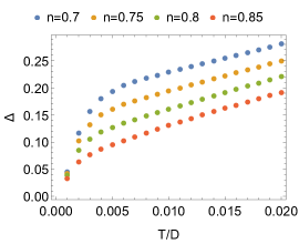
Figure 8: Coefficients of the small frequency expansion of the ECFL Dyson self-energy $\Omega_{\Sigma}$ (8) and $\Delta$ (8) plotted as functions of temperature.

Now we keep $B(\omega,T)$ to $\mathcal{O}(\omega^{2})$ and $A(\omega,T)$ to $\mathcal{O}(\omega)$, which are the lowest orders required to capture all important features of the exact results. Then Eq. (27) and (28) can be simplified as

$$\begin{split}&\sigma_{xx}\simeq\frac{\sigma_{0}F^{0}_{1}}{D^{2}B_{0}}(D^{2}-A_{0}^{2})^{3/2}\Big{(}1-\frac{3\pi^{2}F^{2}_{2}}{F_{1}^{0}}\frac{T^{2}A_{0}A_{1}}{\Delta(D^{2}-A_{0}^{2})}\Big{)},\end{split}$$ (34)

$$\begin{split}&\sigma_{xy}/B\simeq\frac{\sigma_{0}q_{e}F^{0}_{2}}{2D^{2}B_{0}^{2}}{A_{0}(D^{2}-A_{0}^{2})^{3/2}}\\ &\times\Big{(}1+\frac{\pi^{2}F^{2}_{3}}{F_{2}^{0}}\frac{T^{2}A_{1}}{\Delta A_{0}}(1-\frac{3A_{0}^{2}}{D^{2}-A_{0}^{2}})\Big{)}.\end{split}$$ (35)

The coefficients are defined asFmn

$$F_{m}^{n}=\frac{\pi}{4}\int_{-\infty}^{\infty}\frac{dx}{\cosh^{2}(\pi x/2)}\frac{x^{n}}{(1+x^{2})^{m}}.$$ (36)

Using Eqs. (34), (35) and [Fmn, ], we can write

$$\sigma_{xx} \simeq\sigma_{xx,0}(1-\alpha_{xx}),$$ (37)

$$\sigma_{xy} \simeq\sigma_{xy,0}(1-\alpha_{xy}),$$ (38)

with

$$\sigma_{xx,0}=\sigma_{0}\frac{(D^{2}-A^{2}_{0})^{3/2}}{D^{2}}\frac{0.822467}{B_{0}},$$ (39)

$$\sigma_{xy,0}/B=\sigma_{0}q_{e}\frac{A_{0}(D^{2}-A^{2}_{0})^{3/2}}{D^{2}}\frac{0.355874}{B^{2}_{0}},$$ (40)

$$\alpha_{xx}=\frac{A_{1}A_{0}}{D^{2}-A_{0}^{2}}\frac{3.98598\times T^{2}}{\Delta},$$ (41)

$$\alpha_{xy}=-A_{1}\big{(}\frac{1}{A_{0}}-\frac{3A_{0}}{D^{2}-A_{0}^{2}}\big{)}\frac{2.12075\times T^{2}}{\Delta}.$$ (42)

$\sigma_{xx,0}$ agrees with previous worksShastry and Perepelitsky (2016); Ding et al. (2017). $\alpha_{xx(xy)}$ are relative corrections due to $\Delta$ and $A_{1}$ comparing to $\sigma_{xx(xy),0}$. Numerical results of $\alpha_{xx}$ and $\alpha_{xy}$ are shown in Fig. (9). We find that $\lvert\alpha_{xx}\rvert$ is less than $5\%$ even at the highest temperature. However, $\alpha_{xy}$ becomes $\mathcal{O}(1)$ in the GCSM regime. Therefore, we obtain the following asymptotic $\tan\theta_{H}$ by omitting $\alpha_{xx}$:

$$\cot(\theta_{H})\simeq\frac{\cot\theta_{H,0}}{(1-\alpha_{xy})},$$ (43)

$$\cot\theta_{H,0}/B=q_{e}\frac{B_{0}}{0.432691A_{0}}.$$ (44)

We show $\rho_{xx}$ and $\cot(\theta_{H})$ computed from the asymptotic expressions Eq. (37) and (38) in Fig. (9). The asymptotic values are denoted by crosses whereas the results of Eq. (3) and (4) are denoted by solid circles. The numerical results of Eq. (43) recover the second $T^{2}$ regime.

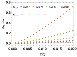
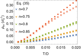
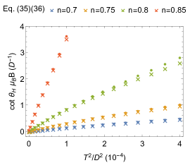
Figure 9: $\alpha_{xx}$ (dashed lines) and $\alpha_{xy}$ (solid symbols) (9), $\rho_{xx}$ (9), $\cot(\theta_{H})$ (9) computed from Eq. (37) and (38) using ECFL results. The asymptotic values are denoted by crosses whereas the ECFL results of Eq. (3) and (4) are denoted by solid circles.

Therefore, we find that the $\alpha_{xy}$ term due to the higher order terms of $A(\omega,T)$ and $B(\omega,T)$ gives rise to the second $T^{2}$ regime of $\cot(\theta_{H})$. Typically such correction is small, such as is the case of $\alpha_{xx}$. The significant difference between $\alpha_{xx}$ and $\alpha_{xy}$ is understood by examining Eq. (41) and (42) more closely. Both $\alpha_{xx}$ and $\alpha_{xy}$ are $\propto A_{1}T^{2}/\Delta$ with slightly different constant factors. Since $A_{0}\ll D$ and almost independent of $T$, we can ignore the $3A_{0}(D^{2}-A_{0}^{2})^{-1}$ term of $\alpha_{xy}$. Hence the difference is mostly determined by a factor

$$\alpha_{xy}/\alpha_{xx}\sim A_{0}^{-2},$$ (45)

which greatly enhances $\alpha_{xy}$.

In the GCFL regime, $\alpha_{xy}$ is negligible, the coefficient of the $T^{2}$ behavior is

$$Q_{FL}=\frac{B\cot(\theta_{H})}{T^{2}}\simeq\frac{\pi^{3}}{0.432691\times q_{e}A_{0}\Omega_{\Sigma}(T\to 0)}.$$ (46)

$\Omega_{\Sigma}(T)$ is almost a constant in the GCFL regime hence approximated by its zero temperature value $\Omega_{\Sigma}(T\to 0)$fitting . In the GCSM regime, both $\Omega_{\Sigma}$ and $\Delta$ becomes linear-in-$T$:

$$\Omega_{\Sigma}(T)\simeq\Omega_{0}(T+T_{\Omega}),$$ (47)

$$\Delta(T)\simeq\Delta_{0}(T+T_{\Delta}),$$ (48)

where $\Omega_{0}(\Delta_{0})$ and $T_{\Omega(\Delta)}$ are fitting parametersfitting . By keeping only the constant term we obtain

$$Q_{SM}\simeq\frac{\pi^{3}}{0.432691\times q_{e}A_{0}\Omega_{0}(T_{\Delta}+T_{\Omega})}.$$ (49)

We compare the actual $Q_{FL}$ and $Q_{SM}$ with Eq. (46) and (49) in Fig. (10).

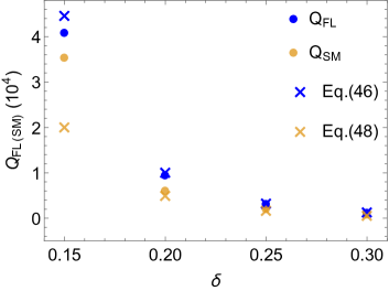
Figure 10: Eq. (46) and (49) (crosses) compared with $Q_{FL}$ and $Q_{SM}$ (solid circles) obtained by fitting the exact $\cot(\theta_{H})$.

According to the above analysis, the second $T^{2}$ behavior of $\cot(\theta_{H})$ is due to the combination of two things:

• the dynamic particle-hole anti-symmetric component of $\rho_{\Sigma}(\omega)$ characterized by the energy scale $\Delta$. Its contribution to transport becomes important when $\pi T$ becomes comparable to $\Delta$;

• the particular form of the transverse transport function $\Phi^{xy}(\epsilon)$ that causes $\Phi^{xy\prime}[A_{0}]/\Phi^{xy}[A_{0}]\propto A^{-1}_{0}$. Without this factor, $\alpha_{xy}$ would be negligible as $\alpha_{xx}$. This particular form of $\Phi^{xy}(\epsilon)$ is due to the particle-hole symmetry of the bare band structure.

VII Discussion

We have shown that Hall constants, Hall angles, optical conductivities, and optical Hall angles calculated by ECFL agree reasonably well with the DMFT results. The differences tend to increase at higher densities and higher temperatures as noted earlierShastry and Perepelitsky (2016).

We focused on the differences in the behavior above and below the Fermi liquid temperature scale $T_{FL}$, i.e., from the GCFL regime to the GCSM regime. Below $T_{FL}$, both $\rho_{xx}$ and $\cot(\theta_{H})$ $\propto T^{2}$. Equivalently, $R_{H}$ has very weak $T$-dependence since $R_{H}=\rho_{xx}/\cot(\theta_{H})$. When $T>T_{FL}$, however, $\cot(\theta_{H})$ passes through a slight downward bend and continues as $T^{2}$ whereas $\rho_{xx}\propto\,T$. The significance of the downward bend is that it signals the crossover to the strange metal regime from the Fermi liquid regime.

We explored the long-standing two-scattering-rate problem by calculating both the optical conductivities and optical Hall angles, and the corresponding scattering rates. Below $T_{FL}$, both $\sigma_{xx}(\omega)$ and $\tan\theta_{H}(\omega)$ exhibit Drude peaks, which is a manifestation of transport dominated by quasiparticles. The corresponding scattering rates can be extracted by fitting to the Drude formula in the appropriate frequency range. Above $T_{FL}$, the Drude peak for $\sigma_{xx}(\omega)$ becomes broadened, i.e., $\sigma_{xx}(0)/\sigma_{xx}(\omega)-1\sim\omega^{2}$ for an even larger range that keeps growing with increasing temperature. In this case, fitting to the Drude formula is still valid, and the scattering rate shows similar trends as a function of temperature as the $dc$ resistivity. For $\theta_{H}(\omega)$, the Drude peak range is very narrow, but nonetheless persists for all temperatures that we study in this work. Similarly, the extracted scattering rate $\Gamma_{H}$ shows similar trends as a function of temperature as the $dc$ Hall angle. At lower dopings and higher temperatures, it seems possible that the Drude peaks of $\theta_{H}(\omega)$ would disappear and the fractional power law would stretch down to nearly $\omega=0$.

By comparing the two optical scattering rates through their ratio, $\Gamma_{H}/\Gamma_{tr}$, we clearly demonstrated that $\Gamma_{H}$ and $\Gamma_{tr}$ are equivalent below $T_{FL}$, but that they quickly become two distinguishable quantities when the system crosses over into the strange-metal region.

By carefully examining the asymptotic expressions of $\sigma_{xx}$ and $\sigma_{xy}$ we established that the different temperature dependence of $\cot(\theta_{H})$ in the GCSM regime is governed by a correction caused by both the dynamical particle-hole anti-symmetric component of $\rho_{\Sigma}(\omega)$ and the particle-hole symmetry of the bare band structure. This correction is turned on when $T$ becomes comparable to $\Delta$, the characteristic energy scale of the anti-symmetric components of $\rho_{\Sigma}(\omega)$.

It would be useful to examine the bend in $\cot(\theta_{H})$ more closely in experiments in cuprate materials, where such a feature is apparently widely prevalent but seems to have escaped comment so far. In particular, one would like to understand better if the longitudinal resistivity and the cotangent Hall angle show simultaneous signatures of a crossover, as the theory predicts.

VIII Acknowledgements

The work at UCSC was supported by the U.S. Department of Energy (DOE), Office of Science, Basic Energy Sciences (BES) under Award # DE-FG02-06ER46319. RŽ acknowledges the financial support from the Slovenian Research Agency (research core funding No. P1-0044 and project No. J1-7259).

References

- Ding et al. (2017) W. Ding, R. Žitko, P. Mai, E. Perepelitsky, and B. S. Shastry, arXiv:1703.02206v2 .
- (2) M. Walter and D. Vollhardt, Phys. Rev. Lett. 62, 324 (1989).
- (3) A. Georges, G. Kotliar, W. Krauth and M. J. Rozenberg Rev. Mod. Phys. 68, 13 (1996).
- Deng et al. (2012) X. Deng, J. Mravlje, R. Zitko, M. Ferrero, G. Kotliar, and A. Georges, Phys. Rev. Lett. 110, 086401 (2012), arXiv:1210.1769 .
- Xu et al. (2013) W. Xu, K. Haule, and G. Kotliar, Phys. Rev. Lett. 111, 036401 (2013), arXiv:1304.7486 .
- Shastry and Perepelitsky (2016) B. S. Shastry and E. Perepelitsky, Phys. Rev. B 94, 045138 (2016), arXiv:1605.08213 .
- Shastry (2011) B. S. Shastry, Phys. Rev. Lett. 107, 056403 (2011), arXiv:1102.2858 .
- (8) R. Žitko, D. Hansen, E. Perepelitsky, J. Mravlje, A. Georges, and B. S. Shastry, Phys. Rev. B 88, 235132 (2013), arXiv:1309.5284 .
- (9) B. S. Shastry and P. Mai, arXiv:1703.08142 (2017).
- Chien et al. (1991) T. Chien, Z. Wang, and N. Ong, Phys. Rev. Lett. 67, 2088 (1991).
- (11) Y. Ando, Y. Kurita, S. Komiya, S. Ono and K. Segawa, Phys. Rev. Letts. 92, 197001 (2004).
- (12) F. F. Balakirev, J. B. Betts, A. Migliori, I. Tsukada, Y. Ando, and G. S. Boebinger, Phys. Rev. Letts. 102, 017004 (2009).
- (13) J. Takeda,T. Nishikawa, M. Sato, Physica C 231, 293 (1994). See esp. Fig. (4).
- Anderson (1991) P. W. Anderson, Phys. Rev. Lett. 67, 2092 (1991).
- Ando et al. (2004) Y. Ando, S. Komiya, K. Segawa, S. Ono, and Y. Kurita, Phys. Rev. Lett. 93, 267001 (2004), arXiv:0403032 [cond-mat] .
- Khurana (1990) A. Khurana, Phys. Rev. Lett. 64, 1990 (1990).
- Pruschke et al. (1993) T. Pruschke, D. L. Cox, and M. Jarrell, Phys. Rev. B 47, 3553 (1993).
- Voruganti et al. (1992) P. Voruganti, A. Golubentsev, and S. John, Phys. Rev. B 45, 13945 (1992).
- Arsenault and Tremblay (2013) L.-F. Arsenault and A.-M. S. Tremblay, Phys. Rev. B 88, 205109 (2013), arXiv:1305.6999 .
- Ziman (1960) J. M. Ziman, “Electrons and phonons: the theory of transport phenomena in solids,” (1960).
- Feng and Jin (2005) D. Feng and G. Jin, in Introd. to Condens. Matter Phys. (WORLD SCIENTIFIC, 2005) pp. 199–229.
- (22) H. Y. Hwang, B. Batlogg, H. Takagi, H. L. Kao, J. Kwo, R. J. Cava, J. J. Krajewski, and W. F. Peck, Jr., Phys. Rev. Lett. 72, 2636 (1994).
- (23) Y. Ando, Y. Kurita, S. Komiya, S. Ono, and K. Segawa, Phys. Rev. Lett. 92, 197001 (2004).
- (24) S. Ono, S. Komiya, and Y. Ando Phys. Rev. B 75, 024515 (2007).
- (25) P. Voruganti, A. Golubentsev and S. John, Phys. Rev. B 45, 13945 (1992).
- Shastry (2012) B. S. Shastry, Phys. Rev. Lett. 109, 067004 (2012).
- (27) Here we give numerical values of here, where is the Reimann zeta function.
-
(28)
Here we give numerical values of , and for respectively:
n 0.7 0.75 0.8 0.85 0.194326 0.10234 0.0443113 0.0135004 5.99932 4.97066 3.79492 2.52377 5.15313 5.58921 5.97819 6.05317 0.0257944 0.0143857 0.00607066 0.000456418 0.0346638 0.0248982 0.0171223 0.0118911 - (29) Ch. Renner, B. Revaz, J.-Y. Genoud, K. Kadowaki, Ø. Fischer, Phys. Rev. Lett. 80, 149 (1998).
- (30) P. W. Anderson, N. P. Ong, J. Phys. Chem. Solid 67, 1 (2006).
- (31) T. Hanaguri, C. Luplen, Y. Kohsaka, D.-H. Lee, M. Azuma, M. Takano, H. Takagi, J. C. Davis, Nature 430, 1001 (2004).
- (32) A. N. Pasupathy, A. Pushp , K. K. Gomes, C. V. Parker, J. Wen, Z. Xu, G. Gu, S. Ono, Y. Ando, A. Yazdani, Science 320, 196 (2008).
- (33) P. A. Casey, J. D. Koralek, N. C. Plumb, D. S. Dessau, P. W. Anderson, Nat. Phys. 4, 210 (2008).
- (34) G.-H. Gweon, B. S. Shastry, G. D. Gu, Phys. Rev. Lett. 107, 056404 (2011).