Millimeter Observations of the disk around GW Ori

The GW Ori system is a pre-main sequence triple system (GW Ori A/B/C) with companions (GW Ori B/C) at $\sim$1 AU and $\sim$8 AU, respectively, from the primary (GW Ori A). The primary of the system has a mass of 3.9 $M_{\odot}$, but shows a spectral type of G8. Thus, GW Ori A could be a precursor of a B star, but it is still at an earlier evolutionary stage than Herbig Be stars. GW Ori provides us an ideal target for experiments and observations (being a “blown-up” upscaled Solar System with a very massive “sun” and at least two “upscaled planets”). We present the first spatially-resolved millimeter interferometric observations of the disk around the triple pre-main-sequence system GW Ori, obtained with the the Submillimeter Array, both in continuum and in the ${}^{12}{\rm CO}\leavevmode\nobreak\ J=2-1$, ${}^{13}{\rm CO}\leavevmode\nobreak\ J=2-1$, and ${\rm C^{18}O}\leavevmode\nobreak\ J=2-1$ lines. These new data reveal a huge, massive, and bright disk in the GW Ori system. The dust continuum emission suggests a disk radius around 400 AU. But, the ${}^{12}{\rm CO}\leavevmode\nobreak\ J=2-1$ emission shows much more extended disk with a size around 1300 AU. Due to the spatial resolution ($\sim$1^′′), we cannot detect the gap in the disk which is inferred from spectral energy distribution (SED) modeling. We characterize the dust and gas properties in the disk by comparing the observations with the predictions from the disk models with various parameters calculated with a Monte Carlo radiative transfer code RADMC–3D. The disk mass is around 0.12 $M_{\odot}$, and the disk inclination with respect to the line of sight is around $\sim$ 35^∘. The kinematics in the disk traced by the CO line emission strongly suggest that the circumstellar material in the disk is in Keplerian rotation around GW Ori. Tentatively substantial ${\rm C^{18}O}$ depletion in gas phase is required to explain the characteristics of the line emission from the disk.

1 Introduction

Spectroscopic and imaging surveys suggest that a majority of young stars are formed in binary/multiple systems (Ghez et al. 1993; Leinert et al. 1993; Ghez et al. 1997; Lafrenière et al. 2008; Kraus et al. 2011). Theoretical and observational studies indicate that the interaction between disks and companions is an efficient mechanism to dissipate disks (Lin & Papaloizou 1993; Cieza et al. 2009; Kraus et al. 2012). Thus, it is very important to investigate disks around the binary or multiple stellar systems, in order to understand disk evolution, as well as planet formation. The triple system GW Ori is an ideal target for such study.

GW Ori is located at $\lambda$ Ori ($\sim$400 pc, Bell et al. 2013), and was revealed as a triple stellar system recently (GW Ori A/B/C, Mathieu et al. 1991; Berger et al. 2011). The primary GW Ori A is a G8 pre-main sequence star with a mass of $\sim$4 $M_{\odot}$, which makes it a very interesting system between Herbig Be stars and classical T Tauri stars (Fang et al. 2014). The close companion GW Ori B was discovered as a spectroscopic binary with an orbital period of $\sim$242 days and a separation of $\sim$1 AU (Mathieu et al. 1991; Fang et al. 2014). The second companion GW Ori C, located at a projected separation of $\sim$8 AU from GW Ori A, was detected with near-infrared interferometric technique (Berger et al. 2011). The sub-millimeter and millimeter observations show that GW Ori is still harboring a massive disk (Mathieu et al. 1995), which is one of the most massive disks around a G-type star. Strong ongoing accretion activity ($\dot{M}_{\rm{acc}}$$\sim$3–4$\times$10^-7 $M_{\odot}$ yr^-1) from the disk to the central star(s) in the GW Ori system was suggested from the $U$-band excess, and strong and broad H$\alpha$ and H$\beta$ emission lines on the spectrum of GW Ori (Calvet et al. 2004; Fang et al. 2014).

In Fang et al. (2014, hereafter Paper I), we presented a study of the inner disk in the GW Ori system based on the infrared data. We reproduced the spectral energy distribution (SED) of GW Ori using disk models with gaps sized 25–55 AU. We found that the SED of GW Ori exhibited dramatic changes on timescales of $\sim$20 yr in the near-infrared bands, which can be interpreted as the change in the amount and distribution of dust particles in the gap due to a “leaky dust filter”. Due to its brightness at submillimeter and millimeter wavelengths, the disk mass and size has been subject to lot of speculation with sizes up to 500 AU radius and masses that could render it gravitational unstable (Mathieu et al. 1995; Schegerer et al. 2009). In this work, we present an investigation of the outer disk around GW Ori using the new millimeter data obtained from the Submillimeter Array (SMA, Ho et al. 2004). These new observations have spatially resolved the disk around GW Ori for the first time. We arrange this paper as follows: In Sect. 2 we describe the observations and data reduction. In Sect. 3 we present our observational results, and in Sect. 4 we describe the disk modeling, and compare the model results with the observations, which are then discussed in 5. We summarize our results in Sect. 6.

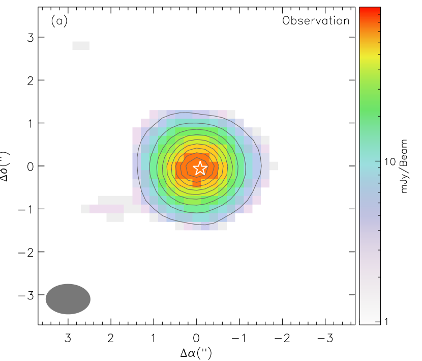
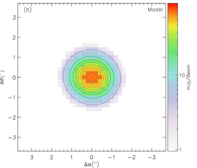
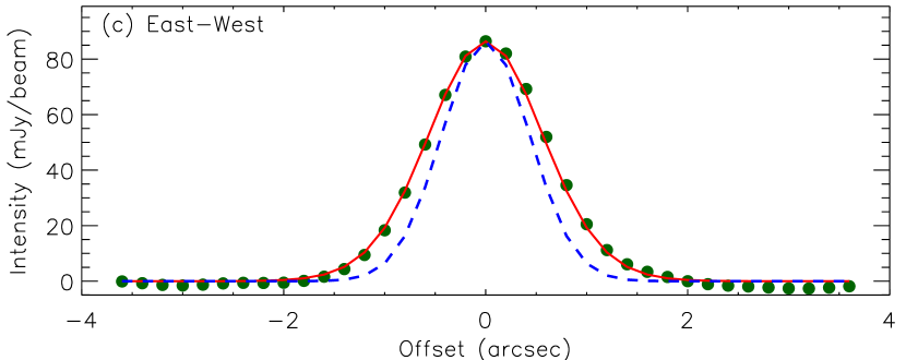
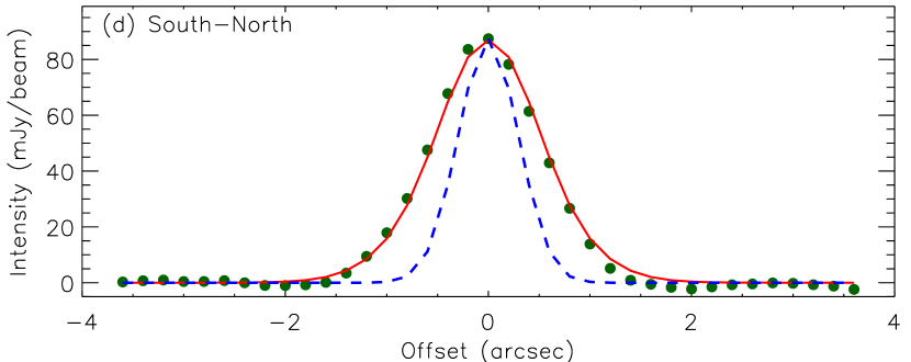
Figure 1: (a) The observed map of the continuum emission observed toward GW Ori at the wavelength of 1.3 mm, with contours (solid lines) drawn at 9.5 mJy beam^-1 (10 $\sigma$) intervals, starting at 4.8 mJy beam^-1 (5 $\sigma$). The synthesized beam is shown in the lower left corner. The position of the central star is indicated with the star symbol. (b) The modeled map of the continuum emission for the GW Ori disk system at the wavelength of 1.3 mm. The contour levels are same as in Panel (a). (c, d) The distribution of the observed intensities (filled circles) along the east-west (c) and north-south (d) direction cross the center of the map compared with the our model (solid lines). The dash lines show the expected profiles for an unresolved object.

2 Observations, data reduction

The object GW Ori was observed with the SMA on January 5, 2010 in the compact configuration with six antennas, on January 19, 2011 in the very extended configuration with six antennas, and February 2, 2011 in the extended configuration with seven antennas. The phase center of the field was RA=05h29m08.38s and Dec=$+11^{\circ}52^{\prime}12.7^{\prime\prime}$ (J2000.0). The SMA has two spectral sidebands, both 4 GHz wide and separated by 10 GHz. The receivers were tuned to 230.538 GHz in the upper sideband ($v_{\rm lsr}$ = 11 km s^-1) with a maximum spectral resolution of 1.1 km s^-1 on the upper sideband and 1.2 km s^-1 on the lower sideband. The system temperatures ($T_{\rm sys}$) were around $\sim$80–200 K during the observation on January 5, 2010, $\sim$100–200 K on January 19, 2011, and $\sim$110–300 K on February 2, 2011. For the compact configuration on January 5, 2010, the bandpass was derived from the quasar 3c273 observations. Phase and amplitude were calibrated with regularly interleaved observations of the quasar 0530+135 (1.7^∘ away from the source). The flux calibration was derived from Titan observations, and the flux scale is estimated to be accurate within 20%. For the very extended configuration on January 19, 2011, the bandpass was derived from the quasar 3c279 observations. Phase and amplitude were calibrated with regularly interleaved observations of the quasar 0530+135 and 0423–013. The flux calibration was derived from Ganymede observations, and the flux scale is estimated to be accurate within 20%. For the extended configuration on February 2, 2011, the bandpass was derived from the quasar 3c279 observations. Phase and amplitude were calibrated with regularly interleaved observations of the quasar 0530+135 and 0423–013. The flux calibration was derived from Titan observations, and the flux scale is estimated to be accurate within 20$\%$.

We merged the three configuration data sets, applied different robust parameters for the continuum and line data, and got the synthesized beam sizes between 1.03^′′ $\times$0.70^′′ (PA$\sim$89.5^∘) and 1.15${}^{\prime\prime}\times 0.83^{\prime\prime}$ (PA$\sim-$88.6^∘), respectively. The rms of 1.3 mm continuum image is 0.96 mJy beam^-1, and the rms of the ¹²CO$\leavevmode\nobreak\ J=2-1$ data is 0.05 Jy beam^-1 at 1.1 km s^-1 spectral resolution, 0.04 Jy beam^-1 at 1.2 km s^-1 spectral resolution for ¹³CO $J=2-1$, and 0.03 Jy beam^-1 at 1.2 km s^-1 spectral resolution for C¹⁸O $J=2-1$. The flagging and calibration was done with the IDL superset MIR (Scoville et al. 1993), which was originally developed for the Owens Valley Radio Observatory and adapted for the SMA. The imaging and data analysis were conducted in MIRIAD (Sault et al. 1995).

3 Observational Results

3.1 Dust continuum emission

In Fig. 1(a), we show the continuum emission map of GW Ori with contours starting at 4.8 mJy beam^-1 (5$\sigma$) and increasing at 9.5mJy beam^-1 (10$\sigma$) intervals. Considering a 20% systematic calibration uncertainty, the integrated continuum flux density in this map is 320$\pm$64 mJy, consistent with the result (255$\pm$60 mJy) in Mathieu et al. (1995). From a two-dimensional Gaussian fit to the image, the full width at half maximum (FWHM) of the continuum emission is 1$\aas@@fstack{\prime\prime}$4($\pm 0\aas@@fstack{\prime\prime}004$)$\times$1$\aas@@fstack{\prime\prime}$3($\pm 0\aas@@fstack{\prime\prime}004$), suggesting that the continuum emission of GW Ori is resolved given the synthesized beam size of 1.03^′′ $\times$0.70^′′. After the deconvolution of the synthesized beam, the FWHM of the continuum emission map is 0$\aas@@fstack{\prime\prime}$9$\times$1$\aas@@fstack{\prime\prime}$1 which is corresponding to 360$\times$400 AU at a distance 400 pc. In Fig. 1(c, d) we show the distribution of the intensities for the the continuum emission map along the east-west and north-south directions cross the center of the map, and the expected distrubutions for an unresolved object according to the spatial resolutions of our observations. We note that the emission of GW Ori along the east-west direction is marginally resolved, but the one along the north-south direction is well resolved.

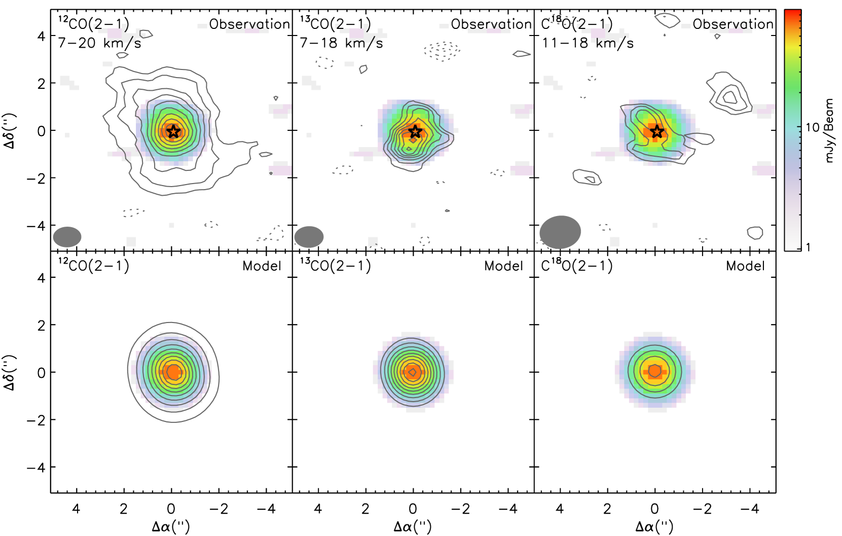
Figure 2: Top panels: The velocity-integrated intensities (contours) for the ${}^{12}{\rm CO}\leavevmode\nobreak\ J=2-1$, ${}^{13}{\rm CO}\leavevmode\nobreak\ J=2-1$, and ${\rm C^{18}O}\leavevmode\nobreak\ J=2-1$ line emission, overlaid on the the continuum emission. For ${}^{12}{\rm CO}\leavevmode\nobreak\ J=2-1$, the intensities are integrated over the velocity range between 6.5 and 20.8 km s^-1, and the contours are drawn at 0.69 Jy beam^-1 km s^-1(3 $\sigma$) intervals, starting at 0.69 Jy beam^-1 km s^-1(3 $\sigma$). For ${}^{13}{\rm CO}\leavevmode\nobreak\ J=2-1$, the intensities are integrated over the velocity range between 7 and 20 km s^-1, and the contours start at 0.48 Jy beam^-1 km s^-1(3 $\sigma$) with an interval of 0.16 Jy beam^-1 km s^-1(1 $\sigma$). For ${\rm C^{18}O}\leavevmode\nobreak\ J=2-1$, the intensities are integrated over the velocity range between 7 and 20 km s^-1, and the contours begin at 0.24 Jy beam^-1 km s^-1(3 $\sigma$), and increase in 0.08 Jy beam^-1 km s^-1(1 $\sigma$) increments. In each panel, the negative contours, shown with the dashed lines, are drawn at $-$1 $\sigma$ intervals, starting at $-$3 $\sigma$. The synthesized beam for each line emission is shown in the lower left corner in each panel. Bottom panels: The modeled velocity-integrated intensities (contours) for the ${}^{12}{\rm CO}\leavevmode\nobreak\ J=2-1$, ${}^{13}{\rm CO}\leavevmode\nobreak\ J=2-1$, and ${\rm C^{18}O}\leavevmode\nobreak\ J=2-1$ line emission, overlaid on the modeled continuum emission, for the GW Ori disk system. The contour levels are same as in the top panels at the corresponding molecular lines.

3.2 Molecular line emission

In the top three panels in Fig. 2 we show the integrated intensity maps of ${}^{12}{\rm CO}\leavevmode\nobreak\ J=2-1$, ${}^{13}{\rm CO}\leavevmode\nobreak\ J=2-1$, and ${\rm C^{18}O}\leavevmode\nobreak\ J=2-1$ lines. The ${}^{12}{\rm CO}\leavevmode\nobreak\ J=2-1$ line emission map shows an elongated structure extended from the north-east to the south-west direction with a single peak coincided with the center of the continuum emission. The ${}^{12}{\rm CO}\leavevmode\nobreak\ J=2-1$ line emission map is clearly spatially resolved. A two-dimensional Gaussian fit to the ${}^{12}{\rm CO}\leavevmode\nobreak\ J=2-1$ integrated intensity map gives an FWHM size of 2$\aas@@fstack{\prime\prime}$5$\times$3$\aas@@fstack{\prime\prime}$4 after the deconvolution of the synthesized beam, corresponding to 890$\times$1300 AU at a distance 400 pc, which is much more extended than the continuum emission map. The ${}^{13}{\rm CO}\leavevmode\nobreak\ J=2-1$ line integrated intensity map of GW Ori is more compact than the ${}^{12}{\rm CO}\leavevmode\nobreak\ J=2-1$ one, and comparable to the continuum emission map. From the disk of GW Ori, we only marginally detect ${\rm C^{18}O}\leavevmode\nobreak\ J=2-1$ line.

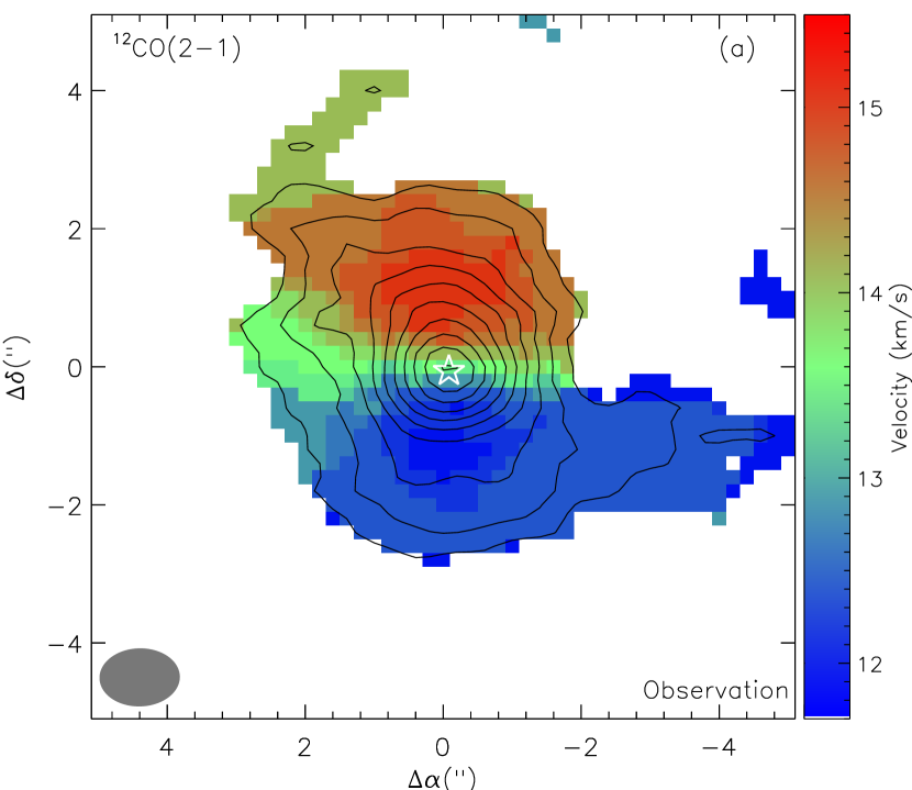
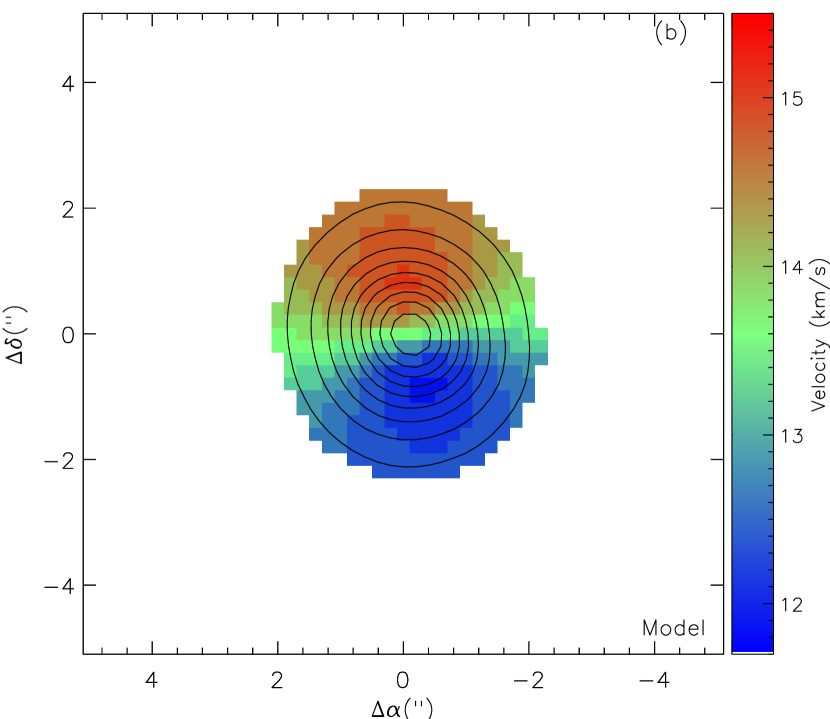
Figure 3: (a) ${}^{12}{\rm CO}\leavevmode\nobreak\ J=2-1$ velocity (1st) moment map. The contours are for the ${}^{12}{\rm CO}\leavevmode\nobreak\ J=2-1$ velocity-integrated intensities (see Fig. 2), starting at 0.69 Jy beam^-1 km s^-1 (3 $\sigma$) with an interval of 0.69 Jy beam^-1 km s^-1 (3 $\sigma$). The synthesized beam is shown in the lower left corner. (b) Same as in Panel (a), but for the predicted map from modeling.

In Fig. 3(a) and Fig. 4(a), we show the ${}^{12}{\rm CO}\leavevmode\nobreak\ J=2-1$ and ${}^{13}{\rm CO}\leavevmode\nobreak\ J=2-1$ velocity (1st) moment maps, respectively, suggesting northern and southern parts of the disk are redshifted and blueshifted with respect to the relative velocity of GW Ori, respectively. Fig. 5 displays the channel maps of ${}^{12}{\rm CO}\leavevmode\nobreak\ J=2-1$ line emission with contours starting at 0.127 Jy beam^-1 (3$\sigma$) with intervals of 0.127 Jy beam^-1. The velocity moment maps and the channel maps are generally consistent with the expected kinematic pattern for gas material in Keplerian rotation with substantial inclination to our line of sight. The disk inclination can be constrained using the position-velocity (PV) diagram of the molecular lines. In Fig. 6(a), we present the PV diagram from the ${}^{12}{\rm CO}\leavevmode\nobreak\ J=2-1$ map along the north-south direction cross the peak of the integrated intensity maps of ${}^{12}{\rm CO}\leavevmode\nobreak\ J=2-1$. In the figure, we plot the expected Keplerian rotation curves for a disk inclined by 20^∘, 40^∘, and 60^∘ around a star with a mass of 3.9 $M_{\odot}$ for comparison. From the comparison, we infer that the disk inclination should be between 20^∘ and 60^∘.

Fig. 5 shows the channel maps of ${}^{12}{\rm CO}\leavevmode\nobreak\ J=2-1$ line emission. In the figure, at the channels with velocities of 12.0 and 13.1 km s^-1, we note a tail structure originating from the outer disk and pointing to the north-western direction. Such a tail is also evident as the blueshifted structure in the ${}^{12}{\rm CO}\leavevmode\nobreak\ J=2-1$ velocity moment map. One explanation for the structure could be the cloud contamination which can be severe for CO lines. If it is the case, it is required that the velocity of the parental cloud around GW Ori is $\sim$1 km s^-1 bluer than GW Ori. A Gaussian fit to the ${}^{12}{\rm CO}\leavevmode\nobreak\ J=2-1$ spectrum at the peak of the integrated line intensity map suggests that the velocity of GW Ori with respect to the local standard of rest (LSR) is around 13.6 km s^-1, and the LSR velocity of the parental cloud of GW Ori is around 12.7 km s^-1 (Lang et al. 2000), which supports the above explanation of the blueshifted tail structure.

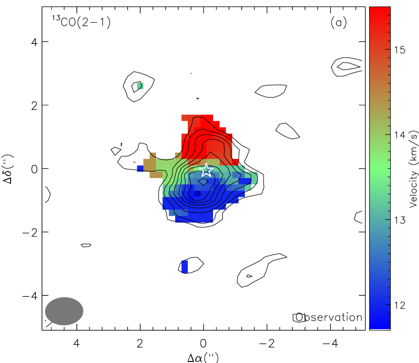
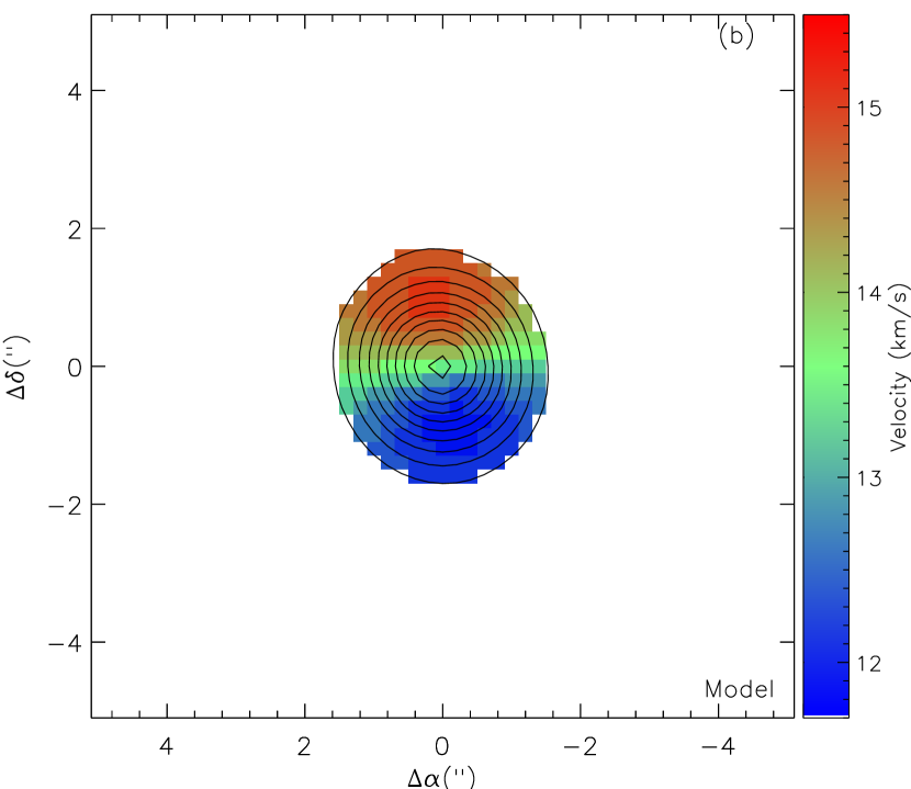
Figure 4: (a) ${}^{13}{\rm CO}\leavevmode\nobreak\ J=2-1$ velocity (1st) moment maps. The contours are for the ${}^{13}{\rm CO}\leavevmode\nobreak\ J=2-1$ velocity-integrated intensities (see Fig. 2), starting at 0.48 Jy beam^-1 km s^-1 (3 $\sigma$) with an interval of 0.16 Jy beam^-1 km s^-1 (1 $\sigma$). The synthesized beam is shown in the lower left corner. (b) Same as in Panel (a), but for the predicted map from modeling.

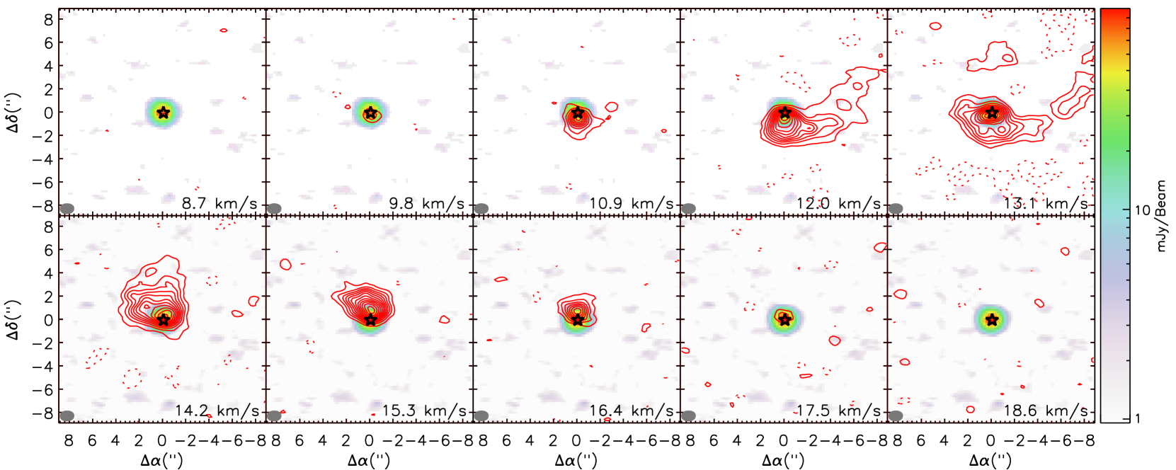
Figure 5: The channel maps of the ${}^{12}{\rm CO}\leavevmode\nobreak\ J=2-1$ emission toward GW Ori. Channels are 1.1 km s^-1 wide with the synthesized beam marked in the bottom left corner. Contour levels are drawn at intervals of 0.127 Jy beam^-1 (3$\sigma$), starting at 0.127 Jy beam^-1. The dashed contours are the negative features with the same contours as the positive ones in each panel. The synthesized beam is shown in the lower left corner in each panel.

4 Disk modeling

In this section, we use a simple disk model to reproduce the SMA observations of GW Ori. Given that our data has low spatial resolution, any model involves a strong simplification of the very complex GW Ori disk system (Fang et al. 2014). Furthermore, the complexity of disks means that the parameter space is highly degenerated and non-continuous (Sicilia-Aguilar et al. 2016). Our aim is thus to explore the global gas and dust content of the GW Ori disk in the light of typical disk models, and to compare it to other similar objects. Any further modeling is beyond the scope of this paper and worth only when higher resolution data becomes available.

4.1 Continuum emission

4.1.1 Parameters for modeling continuum emission

We define a global dust surface density in the same form as in Andrews et al. (2009),

$$\Sigma=\Sigma_{\rm c}\leavevmode\nobreak\ \bigg{(}\frac{R}{R_{\rm c}}\bigg{)}^{-\gamma}\leavevmode\nobreak\ {\rm exp}\Bigg{[}-\bigg{(}\frac{R}{R_{\rm c}}\bigg{)}^{2-\gamma}\Bigg{]},$$ (1)

where $\Sigma_{\rm c}$ is the normalization parameter at the characteristic scaling radius $R_{\rm c}$, and $\gamma$ is the gradient parameter. The above profile, which has been used to successfully model different types of disks in the literature (Andrews et al. 2009, 2011, 2012), is the similarity solution for a simple accretion disk with time-independent viscosity ($\nu$) and $\nu\propto R^{\gamma}$ (Lynden-Bell & Pringle 1974; Hartmann et al. 1998). In this work, we do not take $\Sigma_{\rm c}$ as the free parameter. Instead, we use the disk dust mass ($M_{\rm dust}$), and $\Sigma_{\rm c}$ can be calculated when we set up other parameters about the disk structure. We set $\gamma$ as a free parameter.

We include a vertical gradient in the dust size distribution in disk modelling, to simulate the dust settling in disks. In practice, we use two dust populations: small dust population, and large dust population, as did Andrews et al. (2011). The dust density structure for each dust population in a spherical coordinate system ($R$, $\theta$, and $\phi$) is parameterized as

$$\rho_{\rm small}=\frac{(1-f)\Sigma}{\sqrt{2\pi}Rh}\leavevmode\nobreak\ {\rm exp}\Bigg{[}-\frac{1}{2}\bigg{(}\frac{\pi/2-\theta}{h}\bigg{)}^{2}\Bigg{]},$$ (2)

$$\rho_{\rm large}=\frac{f\Sigma}{\sqrt{2\pi}R\Lambda h}\leavevmode\nobreak\ {\rm exp}\Bigg{[}-\frac{1}{2}\bigg{(}\frac{\pi/2-\theta}{\Lambda h}\bigg{)}^{2}\Bigg{]},$$ (3)

where $\rho_{\rm small}$ is the density for the small dust population, $\rho_{\rm large}$ is the one for the large dust population, and $h$ is the angular scale height. Following Andrews et al. (2011), we assume the large grains are distributed to 20% of the scale height ($\Lambda$=0.2), and account for 85% of the total column ($f$=0.85). We do not explore the parameter space of $\Lambda$ and $f$ since our observational data cannot provide an efficient constraint on them. The angular scale height $h$ is defined as

$$h=h_{\rm c}\leavevmode\nobreak\ \bigg{(}\frac{R}{R_{\rm c}}\bigg{)}^{\Psi},$$ (4)

where $h_{\rm c}$ is the angular scale height at the scaling radius $R_{\rm c}$, and $\Psi$ characterizes the flaring angle of the disk.

In Paper I, we have shown that a gap sized at 25–55 AU needs to be included in the disk model. A small population of tiny dust particles (sizes 0.005–1 $\mu$m) is also needed to distribute in the gap, in order to reproduce the moderate excess emission at near-infrared bands and the strong and sharp silicate feature at 10 $\mu$m on the SED of GW Ori. In this work, we include a dust depletion factor ($\xi_{\rm gap}$) to modify the surface density within the gap. We simply set the gap size $R_{\rm gap}$=45 AU, according to the results in Paper I, since our SMA data cannot provide any constraints on the inner disk. The inner radius of the gap ($R_{\rm in}$) is fixed to be 1.2 AU, which is the orbital semi-major axis of the close companion GW Ori B (see Paper I). When the disk radius $R\leq R_{\rm gap}$, the modified surface density is $\Sigma=\xi_{\rm gap}\Sigma$, where $\Sigma$ is obtained from Equation 1.

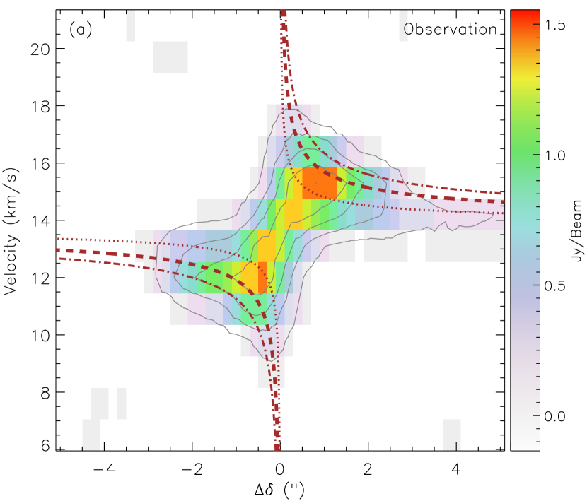
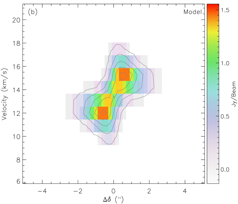
Figure 6: (a) The observed position-velocity diagram from the ${}^{12}{\rm CO}\leavevmode\nobreak\ J=2-1$ map along the north-south direction cross GW Ori. The offset refers to the distance along cut from GW Ori. The contours start at 0.15 Jy beam^-1 (3$\sigma$) with an interval of 0.05 Jy beam^-1 (1$\sigma$). The dotted, dashed, and dash-dotted lines show a Keplerian rotation curve with a central mass of 3.9 $M_{\odot}$ with disk inclinations of 20^∘, 40^∘, and 60^∘, respectively. (b) Same as in Panel (a) but for the modeled position-velocity diagram with a disk inclination of 35^∘.

In the disk models, we use two populations of amorphous dust grains (25% carbon and 75% silicate) with a power-law size distribution with an exponent of $-3.5$ and a minimum size of 0.005 $\mu$m. The maximum size of dust grains is set to be 1 $\mu$m in the gap, as suggested in Paper I, and to be 1 $\mu$m for the small dust population and 1000 $\mu$m for the large dust population in the outer disk ($R>R_{\rm gap}$). In Fig. 7, we show the opacity spectra for the two dust populations derived from Mie calculations.

The stellar parameters adopted in the models are $T_{\rm eff}$=5500 K, $R_{\star}$=7.6 $R_{\odot}$, and $M_{\star}$= 3.9 $M_{\odot}$, taken from Paper I. We use the RADMC–3D code (version  0.40, Dullemond 2012) to do the radiative transfer in the disk models, and vary the free parameters to calculate the continuum emission maps at 1.3 mm and the SEDs. For simplicty, we convolve the model continuum emission maps with the synthetical beam for the SMA continuum emission map to simulate the observations.

4.1.2 Scheme for modeling continuum emission

In order to model the continuum emission from the disk of GW Ori, we have 10 parameters. Among them, the 8 parameters, $R_{\rm in}$, $R_{\rm gap}$, $\xi_{\rm gap}$, $R_{\rm c}$, $\gamma$, $h_{\rm c}$, $\Psi$, and $M_{\rm dust}$, are for the disk structure. As discussed above, we have fixed $R_{\rm in}$=1.2 AU, $R_{\rm gap}$=45 AU. To compare the model results with the observations, we need to know the orientation of the disk with respect to the observer, which can be characterized with two more parameters, the inclination ($i$) of the disk with respect to the line of sight ($i=90^{\circ}$ for edge-on disks), and the position angle (PA) of the disk major axis. The disk of GW Ori is well resolved in the ${}^{12}{\rm CO}\leavevmode\nobreak\ J=2-1$ line. From the integrated intensity map of the ${}^{12}{\rm CO}\leavevmode\nobreak\ J=2-1$ line, we derive an inclination of $\sim$40^∘ and a position angle$\sim$10^∘. In disk modelling, we allow the inclination to change from 30^∘, 40^∘, to 50^∘, and fix position angle to be 10^∘.

The exploration of the parameter spaces is divided into three steps. At the first step, we calculate the continuum emission map at 1.3 mm for a coarse and wide grid of parameters listed in Table 1. Here we fix $\xi_{\rm gap}$=3$\times 10^{-3}$, according to the SED modelling in Paper I, since it only insignificantly affects the 1.3 mm continuum emission modelling. In total, we obtain 9360 modeled 1.3 mm continuum emission maps. We compare the calculated continuum emission maps with the observation, which can efficiently constrain $M_{\rm dust}$ and $R_{\rm c}$. For each model, the goodness of the fit $\chi^{2}_{\rm mm}$ is calculated by

$$\chi^{2}_{\rm mm}=\frac{\frac{1}{N}\sum^{N}_{i=1}(\mu_{i}-\omega_{i})^{2}}{\sigma^{2}}$$ (5)

where $\sigma$ is the noise of the observed 1.3 mm map, $N$ the number of pixels with the values above 3$\sigma$, $\mu$ the modeled data, and $\omega$ the observed data. By comparing with the observations, we obtain sets of disk models providing a good fit which we define as $\chi^{2}_{\rm mm}-\chi^{2}_{\rm mm,\leavevmode\nobreak\ best}<2$ where $\chi^{2}_{\rm mm,\leavevmode\nobreak\ best}$ is the minimum $\chi^{2}_{\rm mm}$ among all the models. In total, we have 102 good-fit models. Then, we calculate the SEDs of the good-fit disk models in the range from 70 $\mu$m to 1.3 mm, and compare them with the one of GW Ori. The goodness of the fit of the SED $\chi^{2}_{\rm SED}$ is calculated by

$$\chi^{2}_{\rm SED}=\frac{1}{N}\sum^{N}_{i=1}\frac{(\mu_{i}-\omega_{i})^{2}}{\sigma_{i}^{2}}$$ (6)

where $N$ is the number of the observed wavelengths, $\mu$ the synthetic flux density, $\omega$ the observed flux density, and $\sigma$ the observational uncertainities. The total goodness of the fit $\chi^{2}_{\rm total}$ is given by

$$\chi^{2}_{\rm total}=\chi^{2}_{\rm mm}+\chi^{2}_{\rm SED}$$ (7)

We derive the ranges for the free parameters of the models providing a good fit with $\chi^{2}_{\rm total}-\chi^{2}_{\rm total,\leavevmode\nobreak\ best}<2$ where $\chi^{2}_{\rm total,\leavevmode\nobreak\ best}$ is the minimum $\chi^{2}_{\rm total}$ among the 102 models. The parameters of the good-fit models are listed in Table 1.

Figure 7: Opacity spectra ($\kappa_{\rm abs}$ for absorption and $\kappa_{\rm sca}$ for scattering) for the small dust population (solid line) and the large dust population (dash line) used in our disk modeling.

Table 1: Coarse grids of the parameters for modeling disk continuum emission.

		Range
Parameters	Input	($\chi^{2}_{\rm total}-\chi^{2}_{\rm total,\leavevmode\nobreak\ best}<2$)
Central star
Effective temperature ($T_{\rm eff}$)	5500 K
Stellar radius	7.5 $R_{\odot}$
Stellar mass ($M_{\star}$)	3.9 $M_{\odot}$
Disk
Inner radius ($R_{\rm in}$)	1.2 AU
Gap size ($R_{\rm gap}$)	45 AU
Dust depletion factor ($\xi_{\rm gap}$)	3$\times 10^{-3}$
Characteristic scaling radius ($R_{\rm c}$)	250, 270, 290, 310, 330, 350, 370, 390  AU	290–350 AU
Surface density gradient parameter ($\gamma$)	0.1, 0.3, 0.5, 0.7, 0.9, 1.1	0.1–0.5
Angular scale height ($h_{\rm c}$)	0.15,0.17,0.19,0.21,0.23	0.15–0.19
$\Psi$	0.1, 0.15, 0.2	0.1–0.2
Disk mass	[1, 1.5, 2, 2.5, 3, 3.5, 4, 4.5, 5, 5.5, 6, 6.7, 7]$\times 10^{-2}\,M_{\star}$	3–3.5$\times 10^{-2}\,M_{\star}$
Disk inclination ($i$)	30∘, 40∘, 50∘	30∘–40∘
Position angle	10∘

At the second step, we refine the grid of parameters with knowledge of the above good-fit models, and list them in Table 2. We repeat the procedure in the first step, but require $\chi^{2}_{\rm mm}-\chi^{2}_{\rm mm,\leavevmode\nobreak\ best}<0.5$ and $\chi^{2}_{\rm total}-\chi^{2}_{\rm total,\leavevmode\nobreak\ best}<0.5$. We obtain the ranges for the free parameters of the models providing a fit with $\chi^{2}_{\rm total}-\chi^{2}_{\rm total,\leavevmode\nobreak\ best}<0.5$. The disk model with minimum $\chi^{2}_{\rm total}$ is considered as the best-fit model.

At the final step, we will constrain the dust depletion factor ($\xi_{\rm gap}$) by fitting the full SED of GW Ori. We calculate a set of model SEDs by varing $\xi_{\rm gap}$ from 1$\times 10^{-3}$ to 1$\times 10^{-2}$ with other parameters from the above best-fit model. Since the change of $\xi_{\rm gap}$ can only obviously vary the shape of the SED within near- and mid-infrared wavelengths, we compare the model SEDs with the observed one within the within the wavelengths ranging from 1 $\mu$m to 37 $\mu$m. We find the model SEDs with $\xi_{\rm gap}=1.5-4\times 10^{-3}$ can reproduce the observations, and the one with $\xi_{\rm gap}=2.5\times 10^{-3}$ can give the best fit to the data. As mentioned before, our model is highly simplified and the low resolution does not allow us to expore in depth the degenerated and non-continuous parameter space of this very complex system. Thus the $\chi^{2}$ approach has to be taken as a tool to measure the goodness of fit, but it cannot be used to derive statistics on the significance of any particular model.

Table 2: Refined Grids of the parameters for modeling disk continuum emission.

		Range
Parameters	Input	($\chi^{2}_{\rm total}-\chi^{2}_{\rm total,\leavevmode\nobreak\ best}<0.5$)	Best-fit
Characteristic scaling radius ($R_{\rm c}$)	290, 300, 310, 320, 330, 340, 350  AU	300–340 AU	320 AU
Surface density gradient parameter ($\gamma$)	0.1, 0.2, 0.3, 0.4, 0.5	0.1–0.4	0.2
Angular scale height ($h_{\rm c}$)	0.15, 0.16, 0.17, 0.18, 0.19	0.15–0.19	0.18
$\Psi$	0.1, 0.15, 0.2	0.1-0.2	0.1
Disk mass	[3.0, 3.1, 3.2, 3.3, 3.4, 3.5]$\times 10^{-2}\,M_{\star}$	3.0–3.4$\times 10^{-2}\,M_{\star}$	3.1$\times 10^{-2}\,M_{\star}$
Disk inclination ($i$)	30∘, 35∘, 40∘	30∘–35∘	35∘

4.2 CO emission

With the parameters of the above best-fit model, we can compute the model map of the ${}^{12}{\rm CO}\leavevmode\nobreak\ J=2-1$ velocity-integrated intensities, and compare it with the observation. However, to calculate the CO emission, one needs to know the gas temperaure distribution in the disk. At the first step, we assume that the gas and dust has equal temperatures, and ignore that CO molecules are frozen out of the gas phase when $T_{\rm gas}<20$ K and that the gas temperatures may be higher than the dust temperatures near the disk surface. The velocity fields of gas material in the disk models are assumed to be Keplerian. The thermal line broadening is automatically included in the RADMC–3D code. Besides it, we also include the turbulent line broadening by assuming a constant linewidth of 0.01 km s^-1 from turbulence. Taking an abundance ratio ${}^{12}{\rm CO}/H_{2}=10^{-4}$, which is the canonical abundance of interstellar medium (ISM), we calculate the ${}^{12}{\rm CO}\leavevmode\nobreak\ J=2-1$ line emission using the RADMC–3D code with an assumption of local thermal equilibrium (LTE) conditions. The resulting maps are simply convolved with the corresponding synthetical beams, and then compared with the observation. We find that the predicted peak intensity of ${}^{12}{\rm CO}\leavevmode\nobreak\ J=2-1$ is about 3 time weaker than the observation. We vary the parameters among the good-fit models listed in Table 2, and the model emission for ${}^{12}{\rm CO}\leavevmode\nobreak\ J=2-1$ line are all 2–3 time weaker than the observation. The previous studies have shown that the gas temperatures could exceed the dust temperatures in the disk surface layers (Qi et al. 2006; Panić et al. 2009), possibly due to additional ultraviolet or X-ray heating from central stars (Glassgold et al. 2004; Jonkheid et al. 2004). In order to reproduce the observed CO emissions of GW Ori, following Andrews et al. (2012), we parameterize the gas temperature as

$$T_{\rm gas}=\left\{\begin{array}[]{l l}T_{\rm atm}+(T_{\rm mid}-T_{\rm atm})\leavevmode\nobreak\ \Bigg{[}{\rm cos}\bigg{(}\frac{\pi}{2}\frac{\pi/2-\theta}{h_{\rm q}}\bigg{)}\bigg{]}^{2\delta}&\quad\text{if $\pi/2-\theta<h_{q}$}\\ T_{\rm atm}&\quad\text{if $\pi/2-\theta\geq h_{q}$}\end{array}\right.$$ (8)

Where $T_{\rm mid}$ is the midplane temperature derived from the RADMC–3D simulations of the dust, $\delta$ describes the steepness of the vertical profile, and $h_{\rm q}=4H_{\rm p}$ where $H_{\rm p}$ is the angular pressure scale height determined from $T_{\rm mid}$. We calculate $H_{\rm p}$ as $H_{\rm p}=(kT_{\rm mid}R/GM_{\star}\mu m_{\rm H})^{1/2}$ where $k$ is the Bolzmann’s constant, $G$ is the gravitational constant, and $\mu=2.37$ is the mean molecular weight of the gas. $T_{\rm atm}$ is the temperature in the disk atmosphere, parameterized as

$$T_{\rm atm}=T_{\rm atm,100\,AU}\bigg{(}\frac{R}{\rm 100\,AU}\bigg{)}^{\zeta}$$ (9)

For gas temperatures, we only set $T_{\rm atm,100\,AU}$ as a free parameter and fix $\delta=2$ and $\zeta$=$-$0.5. We assume that the CO molecules are frozen out of the gas phase when $T_{\rm gas}<20$ K. Since ${}^{12}{\rm CO}\leavevmode\nobreak\ J=2-1$ line emission can be used to constrain the disk inclination better than dust continuum emission, we calculate the ${}^{12}{\rm CO}\leavevmode\nobreak\ J=2-1$ line emission using three disk inclinations, 30^∘, 35^∘, and 40^∘. The ${}^{12}{\rm CO}\leavevmode\nobreak\ J=2-1$ line emission are computed using RADMC-3d assuming non-local thermal equilibrium (non-LTE) conditions for different $T_{\rm atm,100\,AU}$. The result integrated intensity maps of ${}^{12}{\rm CO}\leavevmode\nobreak\ J=2-1$ are simply convolved with the corresponding synthetical beams, and then compared with the observations to characterize $T_{\rm atm,100\,AU}$. For each model, the goodness of the fit $\chi^{2}_{\rm CO}$ is calculated in the similar way as Equation 5, but only for the pixels with values above half of the peak intensity to reduce the possibility of CO contamination by the parental cloud. We also compare the PV diagrams from the observation and from the models to constrain the disk inclination. from a $\chi^{2}$ test, we find a disk model with $T_{\rm atm,100\,AU}$=200$\pm$10 K and $i=35^{\circ}-40^{\circ}$ can fit the observations. In Table 3, we list the best-fit parameter for modeling continuum and gas emission of GW Ori.

4.3 Model results

In our disk models, we have 8 free parameters. The dust depletion factor ($\xi_{\rm gap}$) are mainly constrained by comparing the model SEDs with the observed one at near- and mid-infrared wavelengths, $h_{\rm c}$ can be estimated by fitting the SED at mid- and far-infrared bands, and $M_{\rm dust}$ can be constrained by fitting the SED of GW Ori at submillimeter and millimeter wavelengths and the 1.3 mm continnum emission map. The parameters $R_{\rm c}$ and $\gamma$ are mainly constrained by comparing the model continuum emission map at 1.3 mm with the observations. The disk inclination ($i$) is constrained by fitting the 1.3 mm continuum emission map, the ${}^{12}{\rm CO}\leavevmode\nobreak\ J=2-1$ line emission map, and the PV diagram. And the gas temperature parameter $T_{\rm atm,100\,AU}$ is constrained by fitting the ${}^{12}{\rm CO}\leavevmode\nobreak\ J=2-1$ line emission map. In Table 3, we list the disk model which can satisfactorily reproduce both the 1.3 mm continnum emission, the SED, and the ${}^{12}{\rm CO}\leavevmode\nobreak\ J=2-1$ line emission of GW Ori. In the following, we compare the model results using these parameters with the observations.

Table 3: Disk model parameters for modeling dust and gas emission of GW Ori.

Parameters	Values
Central star
Effective temperature	5500 K
Stellar radius	7.5 $R_{\odot}$
Stellar mass	3.9 $M_{\odot}$
Disk
Inner radius ($R_{\rm in}$)	1.2 AU
Gap size ($R_{\rm gap}$)	45 AU
Dust depletion factor ($\xi_{\rm gap}$)	2.5$\times 10^{-3}$
Characteristic scaling radius ($R_{\rm c}$)	320 AU
Surface density gradient parameter ($\gamma$)	0.2
Angular scale height ($h_{\rm c}$)	0.18
$\Psi$	0.1
Disk mass	0.12 $M_{\odot}$
$T_{\rm atm,100\,AU}$	200 K
Power index for $T_{\rm atm}$ ($\zeta$)	$-$0.5
$\delta$	2
Disk inclination ($i$)	35∘
Position angle	10∘

In Fig. 1(b), we show the model continuum emission at 1.3 mm. In Fig. 1(c, d), we compare the distribution of the intensity along the east-western and south-northern direction across the center of the map, respectively, from the model. The model results can fit the observations well. In Fig. 8, we compare the model SED with the observed one. The observed SED in the figure is the type 1 SED for GW Ori in Paper I, and constructed using the $UBVR_{\rm C}I_{\rm C}$ photometry from Calvet et al. (2004), the $JHK_{\rm s}$ photometry from the 2MASS survey (Skrutskie et al. 2006), the photometry at 3.4, 4.6, 12, and 22 $\mu$m from the WISE survey (Wright et al. 2010), the photometry at 9 and 18 $\mu$m from the AKARI survey (Ishihara et al. 2010), the MIPS 70 $\mu$m photometry from Paper I, the fluxes at 350, 450, 800, 850, 1100, 1360 $\mu$m from Mathieu et al. (1995), and the 5$-$37 $\mu$m  low-resolution IRS spectrum from paper I. In Fig. 8, it can be seen that our simple disk model can well reproduce the observed SED of GW Ori. In Fig. 2, we show the model map of the ${}^{12}{\rm CO}\leavevmode\nobreak\ J=2-1$ velocity-integrated intensities calculated with the parameters in Table 3, which reproduces the observation very well. Figure 3(b) displays the model ${}^{12}{\rm CO}\leavevmode\nobreak\ J=2-1$ velocity moment map, and Fig. 6(b) shows the model PV diagram for the ${}^{12}{\rm CO}\leavevmode\nobreak\ J=2-1$ lines.

Using the disk parameters listed in Table 3, and taking the typical abundances of ISM for ${}^{13}{\rm CO}$ and ${\rm C^{18}O}$, ${}^{13}{\rm CO}/{\rm H_{2}}=1.43\times 10^{-6}$ and ${\rm C^{18}O}/{\rm H_{2}}=1.82\times 10^{-7}$, i.e. ${}^{12}{\rm CO}/^{13}{\rm CO}$=70 and ${}^{12}{\rm CO}/{\rm C^{18}O}$=550 (Wilson & Rood 1994), we calculate the the predicted emission of the ${}^{13}{\rm CO}$ and ${\rm C^{18}O}$ lines using RADMC–3D assuming Non-LTE conditions. We note the predicted line emission of ${}^{13}{\rm CO}\leavevmode\nobreak\ J=2-1$ is consistent with the observations (see Fig. 2 and Figure 4(b)), but the model line emission of ${\rm C^{18}O}\leavevmode\nobreak\ J=2-1$ is three time stronger than the observational data. A simple solution to reduce the model line emission is to decrease the abundance of ${\rm C^{18}O}$ in gas phase, which can be due to the real reduction in their abundances or more freezing than we assumed. We find that a satisfactory fit to the SMA data required that ${\rm C^{18}O}/{\rm H_{2}}\sim 2.3\times 10^{-8}$. In Fig. 2, we show the model map of ${\rm C^{18}O}\leavevmode\nobreak\ J=2-1$ velocity-integrated intensities calculated using the above abundances. Such global ${\rm C^{18}O}$ gas-phase depletion in circumstellar disks has been suggested before (Dutrey et al. 1994, 1996; Dartois et al. 2003; Isella et al. 2007), which can be due to a selective photodissociation of CO and its isotopes in disks (Visser et al. 2009). However, we must stress that the constraint on the abundance of ${\rm C^{18}O}$ in the disk of GW Ori based on the SMA data is just tentative since the detection of ${\rm C^{18}O}$ is marginal. Furthermore, an underestimate of the dust absorption of the line emission in the disk modelling or over-subtraction of continuum around ${\rm C^{18}O}\leavevmode\nobreak\ J=2-1$ could complicate the issue.

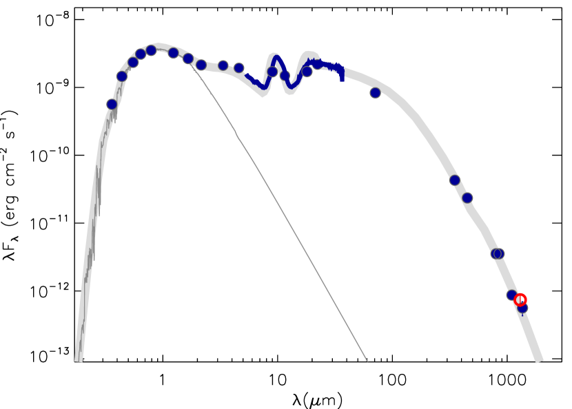
Figure 8: The observed SED of GW Ori. The broad band photometry is shown with the filled circles, and the IRS spectrum of this source is displayed in solid line. The open circle show the flux from our SMA observations. The thick gray line shows our model SED. The photospheric emission level is indicated with a thin gray curve.

We have shown that our disk model can reproduce the SMA observations of GW Ori. However, multi-parameter disk models are known to be highly degenerated and non-continuous. In addition, there are other sources of uncertain in disk modeling. The dust growth and settling in disks can change the dust properties vertically and radially (Birnstiel et al. 2010, 2012). And it is unknown whether the gas and dust are well mixed in the GW Ori disk, and the gas-to-dust ratio may vary vertically and radially (Birnstiel et al. 2010). All these put strong limitations on the interpretations of the results from our disk modeling. The inferred disk masses can be strongly dependent on the assumed dust model (size distribution) and gas-to-dust ratio. In addition, it should be expected that the structure of the disk, vertical scale height, dust distribution, and heating may differ from typical cases due to the interaction between the two companions and the very massive disk in GW Ori.

5 Discussion

The disk inclination of GW Ori is constrained by the gas kinematics in the disk traced by the ${}^{12}{\rm CO}$ line, which gives an intermediate inclination ($\sim$35^∘). In Paper I we have estimated the inclination of the stellar rotation axis of the primary star (GW Ori A), which is around 35–50^∘. Thus the stellar rotation axis of GW Ori A and the disk spin axis could be aligned. It is still unclear if the the binary orbital plane and the disk is aligned in the GW Ori system. If it is the case, the mass of the close companion GW Ori B is estimated to be 0.44 $M_{\odot}$ using the minimum companion mass ($m_{2}{\rm sin}\leavevmode\nobreak\ i_{*}=0.25$, $i_{*}$ is the inclination of the orbit) derived in Paper I. In this case, the expected $H$-band flux ratio between the primary GW Ori A (3.9 $M_{\odot}$) and GW Ori B (0.44 $M_{\odot}$) is 30:1 at age of $\sim$0.9 Myr from the pre-main-sequence evolutionary tracks of Siess et al. (2000). On the contrary, the near-infrared interferometric observations show that the two stellar components may have near-equal $H$-band fluxes (2:1), which requires a low inclination of the orbit ($\sim$10^∘) for GW Ori to have a massive close companion GW Ori B. However, an inclined orbit of a massive companion can drastically disturb the disk (Larwood et al. 1996). In addition, Shevchenko et al. (1998) detected the eclipses toward GW Ori during 1987-1992, which may suggest a nearly edge-on inclination of the the orbit for GW Ori A/B. However, recent observation with Kepler/K2 observations detect many quasi-periodic or aperiodic dimming events from young stars with disks, which are not edge-on, and could be due to inclined and variable inner dust disk warps (Ansdell et al. 2016a, b; Scaringi et al. 2016). Thus, an intermediate disk inclination of GW Ori does not contradict with the observation from Shevchenko et al. (1998).

6 Summary

Using the SMA we have mapped the disk around GW Ori both in continuum and in the $J=2-1$ transitions of ${}^{12}{\rm CO}$, ${}^{13}{\rm CO}$, and ${\rm C^{18}O}$. The dust and gas properties in the disk are obtained by comparing the observations with the predictions from disk models with various parameters.

We find a clear evidence that the circumstellar material in the disk is in Keplerian rotation around GW Ori with a disk inclination of $\sim$35^∘.

We present a disk model which can reproduce the dust continuum and line emission of CO and its isotopes from the disk of GW Ori. To reproduce the line emission of ${\rm C^{18}O}$, we may need the substantially depleted abundances of ${\rm C^{18}O}$ in gas phase.

GW Ori is one of the most remarkable disks regarding its mass, and one of the most remarkable stellar systems (a massive G8 star with two companions). This object is bright at the whole electromagnetic spectrum and well studied, and an ideal target for future observations with ALMA.