Model-independent constraints on hadronic form factors with above-threshold poles

Abstract

Model-independent constraints on hadronic form factors, in particular those describing exclusive semileptonic decays, can be derived from the knowledge of field correlators calculated in perturbative QCD, using analyticity and unitarity. The location of poles corresponding to below-threshold resonances, i.e., stable states that cannot decay into a pair of hadrons from the crossed channel of the form factor, must be known a priori, and their effect, accounted for through the use of Blaschke factors, is to reduce the strength of the constraints in the semileptonic region. By contrast, above-threshold resonances appear as poles on unphysical Riemann sheets, and their presence does not affect the original model-independent constraints. We discuss the possibility that the above-threshold poles can provide indirect information on the form factors on the first Riemann sheet, either through information from their residues or by constraining the discontinuity function. The bounds on form factors can be improved by imposing, in an exact way, the additional information in the extremal problem. The semileptonic $K\to\pi\ell\nu$ and $D\to\pi\ell\nu$ decays are considered as illustrations.

I Introduction

Since the pioneering works of Meiman [1] and Okubo [2, 3], it has been known that nontrivial constraints on hadronic form factors can be derived from the knowledge of suitably related field correlators. The method was reconsidered in [4] within the modern theory of strong interactions, where the correlators relevant for the bounds on the $K_{\ell 3}$ form factors were evaluated in the deep Euclidean region by using perturbative QCD.

The method exploits unitarity and positivity of the spectral function, and converts a dispersion relation for a correlator of two currents into an integral condition along the unitarity cut (i.e., above the lowest production threshold of particles coupled to the currents) for the modulus-square of the form factors parametrizing the relevant matrix elements in the unitarity sum. From this condition and the analyticity properties of the form factors as functions of energy, one can derive, with standard techniques of complex analysis [5, 6], constraints on the values of the form factors and their derivatives at points inside the analyticity domain.

Many applications of this approach to heavy-quark form factors describing $B\to D^{(*)}\ell\nu$ semileptonic decays, to heavy-to-light form factors involved in $B\to\pi\ell\nu$ or $D\to\pi\ell\nu$ decays, or to the light-meson form factors, have been performed in the last 20 years [7, 8, 9, 10, 11, 12, 13, 14, 15, 16, 17, 18, 19, 20, 21, 22, 23, 24, 25, 26] (for a review of earlier literature see [27]). A similar formalism has been applied also to the electromagnetic form factors of the pion [28, 29, 30, 31] and proton [32], to the $\pi\omega$ form factor [33, 34], and to heavy baryons [35].

The presence of singularities below the unitarity threshold modifies the derivation of the bounds. The method can be adapted to include in an exact way the discontinuity across an unphysical cut below the unitarity branch point, present in some cases, related to lighter particles that can couple to the current [33, 34]. A pole situated below the unitarity threshold, of known position but unknown residue, can be also accounted for in an optimal way with the technique of Blaschke factors [12, 13]. In such a case, the presence of the pole leads to a weakening of the constraints.

Recently, the possible effect of resonances situated above the unitarity threshold, close to the physical region, was discussed in [36]. As known from general principles of quantum field theory [37], the unstable particles are associated to complex poles in the energy plane. Such poles cannot appear on the first Riemann sheet of the complex plane, and instead are situated on the second or higher Riemann sheets. The argument used in [36] was based on the remark that a complex pole on the second sheet close to the real axis produces a local increase of the modulus of the form factor on the unitarity cut. The same increase can be obtained however with a complex singularity of the same position, but situated on the first Riemann sheet. Therefore, in [36] it was argued that the effect of an above-threshold singularity can be mimicked through a complex pole on the first Riemann sheet, near the physical region. The latter can be treated with the standard technique of Blaschke factors, much like the subthreshold poles. In this way, Ref. [36] estimated the physical effect of the presence of above-threshold resonances.

In the present paper, we consider the question whether the form-factor parametrizations can be improved if some knowledge on the above-threshold poles is provided. We start with a brief review of the technique of model-independent constraints, presenting in particular the stronger constraints obtained with some additional information outside the semileptonic decay range. In Sec. III we argue first that the presence of an above-threshold pole does not affect the original bounds in the semileptonic region. Then we investigate whether, from the presence of an above-threshold resonance, one can obtain some information on the form factor on the physical sheet and show that, in some cases, the bounds can be improved by implementing additional information of this type. In particular, we find that the most practical constraints arise from mapping the effect of the above-threshold resonance to the phase of the form factor along the cut. Our conclusions are given in the last section. In a short Appendix, we discuss the connection between the first two Riemann sheets and the canonical variable $z$ used for solving the extremal problem.

II Model-independent constraints on hadronic form factors

We present below, following the review [27] and the recent paper [36], the main steps relevant for the derivation of constraints on the form factor parametrizations. As in [36], we concentrate in particular on the form factors relevant for the semileptonic decays of pseudoscalar mesons. We consider the heavy-to-light ($Q\to q$) vectorlike ($V$, $A$, or $V\!-\!A$) quark-transition current

$$J^{\mu}\equiv\bar{Q}\Gamma^{\mu}q\,,$$ (1)

and the two-point momentum-space Green’s function $\Pi_{J}^{\mu\nu}$ separated into manifestly spin-1 ($\Pi_{J}^{T}$) and spin-0 ($\Pi_{J}^{L}$) terms:

$$\Pi_{J}^{\mu\nu}(q)\equiv i\!\int\!d^{4}\!x\,e^{iqx}\left<0\left|TJ^{\mu}(x)J^{\dagger\nu}(0)\right|0\right>$$

$$=\frac{1}{q^{2}}\left(q^{\mu}q^{\nu}-q^{2}g^{\mu\nu}\right)\Pi^{T}_{J}(q^{2})+\frac{q^{\mu}q^{\nu}}{q^{2}}\Pi^{L}_{J}(q^{2})\,.$$ (2)

The functions $\Pi^{T,L}_{J}$ satisfy dispersion relations with positive spectral functions, expressed by unitarity in terms of contributions from a complete set of hadronic states. From the asymptotic behavior predicted by perturbative QCD, it follows that the dispersion relations require subtractions (one for $\Pi^{L}_{J}$ and two for $\Pi^{T}_{J}$). The subtraction constants disappear by taking the derivatives:

$$\chi^{L}_{J}(q^{2})\equiv\frac{\partial\Pi^{L}_{J}}{\partial q^{2}}=\frac{1}{\pi}\int_{0}^{\infty}\!dt\,\frac{{\rm Im}\,\Pi^{L}_{J}(t)}{(t-q^{2})^{2}}\,,$$

$$\chi^{T}_{J}(q^{2})\equiv\frac{1}{2}\frac{\partial^{2}\Pi^{T}_{J}}{\partial(q^{2})^{2}}=\frac{1}{\pi}\int_{0}^{\infty}\!dt\,\frac{{\rm Im}\,\Pi^{T}_{J}(t)}{(t-q^{2})^{3}}\,.$$ (3)

Perturbative QCD can be used to compute the functions $\chi^{\vphantom{\dagger}}_{J}(q^{2})$ at values of $q^{2}$ far from the region where the current $J$ can produce manifestly nonperturbative effects like pairs of hadrons. For heavy quarks, $Q=c$ or $b$, a reasonable choice is $q^{2}=0$, while for $Q=s$ a spacelike value, like $q^{2}=-1\,\text{GeV}^{2}$ or $q^{2}=-2\,\text{GeV}^{2}$, is necessary.

The spectral functions ${\rm Im}\,\Pi_{J}$ are evaluated by unitarity, inserting into the unitarity sum a complete set of states $X$ that couple the current $J$ to the vacuum:

$${\rm Im}\,\Pi^{\mu\nu}_{J}(q^{2})=\frac{1}{2}\sum_{X}(2\pi)^{4}\delta^{4}(q-p_{X})\left<0\left|J^{\mu}\right|\!X\right>\left<X\!\left|J^{\dagger\nu}\right|0\right>.$$ (4)

For our purpose, it is enough to take $X$ to be the lightest meson pair in which one of them (of mass $M$) contains a $Q$ quark and the other (of mass $m$) contains a $\bar{q}$, and use the positivity of the higher-mass contributions. This choice gives a rigorous lower bound on the spectral functions, in terms of the vector or scalar form factors that parametrize the matrix elements of the current. Using the standard notation

$$t_{\pm}\equiv(M\pm m)^{2}\,,$$ (5)

the inequality for the transverse polarization $\Pi^{T}_{J}$ can be written as

$$\frac{1}{\pi\chi^{T}_{J}(q^{2})}\int_{t_{+}}^{\infty}\!dt\frac{w(t)\,|F(t)|^{2}}{(t-q^{2})^{3}}\leq 1\,,$$ (6)

where $t_{+}$ is the unitarity threshold, $F(t)$ is the vector form factor, and $w(t)$ is a simple, nonnegative function, expressed as a product of phase-space factors depending upon $t_{+}$ and $t_{-}$. An analogous expression holds for $\Pi^{L}_{J}$ and the scalar form factor.

Using the standard dispersion techniques in quantum field theory [38], one can prove that the semileptonic form factors are in general analytic functions in the complex $t$ plane, with a unitarity cut along the real axis from $t_{+}$ to $\infty$. In some cases, as in $B\to D\ell\nu$ and $B\to\pi\ell\nu$, the form factors may also exhibit poles situated on the real axis below the unitarity threshold $t_{+}$. No analogous poles are present in the form factors relevant in $K\to\pi\ell\nu$ and $D\to\pi\ell\nu$ decays. All the form factors in semileptonic decays satisfy in addition the Schwarz reflection condition, written generically as $F(t^{*})=F^{*}(t)$. The form factors are therefore real on the real $t$ axis below $t_{+}$, in particular in the semileptonic region $0\leq t\leq t_{-}$, where they can be measured from the decay rates.

As shown in the pioneering papers [1, 2, 3, 4], one can obtain constraints on the form-factor parametrizations in the semileptonic region, using their analyticity properties and the boundary condition (6). In order to exploit this condition, it is convenient to map the cut $t$ plane onto the unit disk in the complex $z$ plane defined by the conformal mapping

$$z\equiv\tilde{z}(t;t_{0})\equiv\frac{\sqrt{t_{+}-t_{0}}-\sqrt{t_{+}-t}}{\sqrt{t_{+}-t_{0}}+\sqrt{t_{+}-t}}\,,$$ (7)

which maps the cut $t$ complex plane onto the interior of the unit disk, such that the branch point $t_{+}$ in mapped onto $z=1$ and the two edges of the unitarity cut $t\geq t_{+}$ map to the boundary $|z|=1$. Moreover, $z$ is real for $t\leq t_{+}$. The choice of the free parameter $t_{0}$ in (7), which represents the point mapped onto the origin of the $z$ plane, $\tilde{z}(t_{0};t_{0})=0$, will be discussed below.

In the variable $z$, the inequality (6) is written in the equivalent form

$$\frac{1}{2\pi i}\oint_{C}\frac{dz}{z}|\phi(z)F[\tilde{t}(z;t_{0})]|^{2}\leq 1\,,$$ (8)

where

$$\tilde{t}(z;t_{0})=\frac{4zt_{+}+t_{0}(1-z)^{2}}{(1+z)^{2}}$$ (9)

is the inverse of (7), and $\phi(z)$ is an outer function, defined in complex analysis [5] as an analytic function lacking zeros in $|z|<1$. In our case, the function $\phi(z)$ is defined by specifying its modulus

$$|\phi(z)|^{2}=\ \frac{w[\tilde{t}(z;t_{0})]}{|d\tilde{z}(t;t_{0})/dt|\,\chi^{T}(q^{2})[\tilde{t}(z;t_{0})-q^{2}]^{3}}\,,$$ (10)

on the boundary $z=e^{i\theta}$ of the unit disk. Then the function for $|z|<1$ can be reconstructed from its modulus on the boundary by the representation [5]

$$\phi(z)=\exp\left[\frac{1}{2\pi}\int_{0}^{2\pi}{\rm d}\theta\,\frac{e^{i\theta}+z}{e^{i\theta}-z}\,\ln|\phi(e^{i\theta})|\right].$$ (11)

In particular cases of physical interest, $\phi(z)$ can be obtained in closed form, as a product of simple analytic functions (see [27, 36]).

From the boundary condition (8), one can derive constraints on the form factor $F(t)$ at points inside the analyticity domain, in particular in the semileptonic region. It is important to emphasize that the use of the outer function in (8) ensures the constraints are optimal. Assume first that the form factor $F(t)$ has no singularities below the unitarity threshold $t_{+}$, being an analytic function of real type [$F^{*}(t)=F(t^{*})$] in the cut $t$ plane, or equivalently in the unit disk $|z|<1$ (as mentioned above, this is the case for the $K\pi$ or $D\pi$ form factors). Then, expanding as:

$$F(z)\equiv F[\tilde{t}(z;t_{0})]=\frac{1}{\phi(z)}\sum_{k=0}^{\infty}a_{k}z^{k}\,,$$ (12)

where the coefficients $a_{k}$ are real, the condition (8) reads:

$$\sum_{k=0}^{\infty}a_{k}^{2}\leq 1\,.$$ (13)

This inequality, which is valid also for any finite sum of terms, was used in many studies to strongly constrain the parameters used in the fits to semileptonic data or for estimating the truncation error [15, 16, 17, 19, 21, 22, 23, 24]. As discussed in several papers, the truncation error is minimized by choosing the parameter $t_{0}$ such that the semileptonic range $0\leq t\leq t_{-}$ is mapped onto an interval $(-z_{\rm max},z_{\rm max})$ symmetric around the origin in the $z$ plane. This method allowed a high-precision determination of the elements $V_{us},V_{cb}$, and $V_{ub}$ of the CKM matrix from exclusive semileptonic decays.

The constraints on the Taylor series coefficients $a_{k}$ become stronger if some additional information on the form factor outside the semileptonic range is available. The general condition involving an arbitrary number of coefficients $a_{k}$ and the values of $F(z)$ at an arbitrary number of points inside the unit disk has been derived using several methods and can be found in [27].

For the discussion in the next section, it is of interest to give the form of the constraint when one knows the values of the form factor $F(z)$ at two complex-conjugate points, which we denote as $z_{p}$ and $z_{p}^{*}$, with $|z_{p}|<1$. Since the functions satisfy the Schwarz reflection property, one has $F(z_{p}^{*})=F^{*}(z_{p})$. Using, as in [27], the technique of Lagrange multipliers for imposing the additional constraints at $z_{p}$ and $z_{p}^{*}$, a straightforward calculation gives the inequality

$$\sum_{k=0}^{K-1}a_{k}^{2}\leq 1-{\cal F}(z_{p},\xi),$$ (14)

where ${\cal F}$ is defined as

$${\cal F}(z_{p},\xi) \!\!=\!\! \frac{2(1-|z_{p}|^{2})^{2}|1-z_{p}^{2}|^{2}}{|z_{p}|^{4K}(z_{p}-z_{p}^{*})^{2}}$$

$$\!\!\times\!\! \left[{\text{Re}}\left(\frac{\xi^{2}z_{p}^{*2K}}{1-z_{p}^{*2}}\right)-\frac{|\xi|^{2}|z_{p}|^{2K}}{1-|z_{p}|^{2}}\right]\,,$$

in terms of the point $z_{p}$ and the complex quantity

$$\xi=\phi(z_{p})F(z_{p})-\sum_{k=0}^{K-1}a_{k}z_{p}^{k}.$$ (16)

The inequality (14) defines an allowed domain for first $K$ coefficients $a_{k}$ in terms of the input complex value $F(z_{p})$ entering the variable $\xi$. One can check from (II) that the function ${\cal F}$ is positive for $|z_{p}|<1$ and arbitrary values of $a_{k}$ and $F(z_{p})$. Therefore, the domain defined by (14) is smaller than that given by the condition

$$\sum_{k=0}^{K-1}a_{k}^{2}\leq 1$$ (17)

derived from (13). As expected, knowledge of the value $F(z_{p})$ improves the constraints on the parameters in the semileptonic region. We note, however, that the improvement is small if the point $z_{p}$ is close to the boundary of the unit disk, since ${\cal F}$ is small for $|z_{p}|$ close to 1.

Another additional piece of information that can improve the constraints is knowledge of the phase of the form factor along a part of the unitarity cut. In some cases, as for the pion electromagnetic form factor or the $K_{\ell 3}$ form factors, the phase is related by Fermi-Watson theorem [39, 40] to the phase shift of the corresponding elastic scattering amplitude, which is known with precision, for instance from the solution of Roy equations [41]. In the present context (as discussed in the next section), it is of interest to note that one can approximately obtain the phase on a part on the cut using the mass and width of a nearby resonance.

Using this information as an additional constraint leads to a modified optimization problem, solved for the first time for the $K_{\ell 3}$ form factors in [42]. Several generalizations have been discussed more recently in [20, 21, 27]. For completeness, we give below the constraint on the first $K$ coefficients $a_{k}$ when the phase $\arg F(t)$ is known on the region $0\leq t\leq t_{\text{in}}$ (for the derivation, see Sec. 4 of the review [27]).

We denote by

$$\zeta_{\rm in}\equiv\tilde{z}(t_{\text{in}};t_{0})=e^{i\theta_{\rm in}}$$ (18)

the image on the unit circle in the $z$ plane of the point $t_{\text{in}}+i\epsilon$ situated on the upper edge of the cut [the point $t_{\text{in}}-i\epsilon$ being mapped onto $\exp(-i\theta_{\rm in}$)]. Then the domain allowed for the coefficients $a_{k}$ is given by

$$\sum_{k=0}^{K-1}a_{k}^{2}+\frac{1}{\pi}\sum_{k=0}^{K-1}a_{k}\int\limits_{-\theta_{\rm in}}^{\theta_{\rm in}}{\rm d}\theta\,\lambda(\theta)\sin\left[k\theta-\Phi(\theta)\right]\leq 1,$$ (19)

where

$$\Phi(\theta)=\arg[F(e^{i\theta})]+\arg[\phi(e^{i\theta})]\,,$$ (20)

and $\lambda(\theta)$ is the solution of the integral equation

$$\sum_{k=0}^{K-1}a_{k}\sin[k\theta-\Phi(\theta)]=\lambda(\theta)-\frac{1}{2\pi}\!\int\limits_{-\theta_{\rm in}}^{\theta_{\rm in}}{\rm d}\theta^{\prime}\lambda(\theta^{\prime})\,{\cal K}_{\Phi}(\theta,\theta^{\prime}),$$ (21)

for $\theta\in(-\theta_{\rm in},\theta_{\rm in})$, where the kernel is defined as

$${\cal K}_{\Phi}(\theta,\theta^{\prime})\equiv\frac{\sin[(K-1/2)(\theta-\theta^{\prime})-\Phi(\theta)+\Phi(\theta^{\prime})]}{\sin[(\theta-\theta^{\prime})/2]}\,.$$ (22)

The inequality (19) describes an allowed domain for $a_{k}$ that is smaller than the original domain (17), which represents the improvement introduced by knowledge of the phase on a part of the unitarity cut.

In the above derivations, the crucial role was played by the fact that the form factor is analytic in the cut $t$ plane. As discussed above, the form factors relevant for $K\to\pi\ell\nu$ and $D\to\pi\ell\nu$ decays do not have subthreshold singularities, while the form factors involved in $B\to D^{(*)}\ell\nu$ and $B\to\pi\ell\nu$ decays have subthreshold poles, corresponding to particles stable with respect to strong decays into $\bar{B}D$ and $\bar{B}\pi$, respectively.

As remarked for the first time in [12, 13], it is possible to derive constraints on the form factor even if the residue of the pole is not known. Denoting by $z_{p}$ the position of the pole in the $z$-variable, the inclusion of the pole can be done in an optimal way with respect to the condition (8) by using a so-called Blaschke factor [5]:

$$B(z;z_{p})\equiv\frac{z-z_{p}}{1-zz_{p}^{*}}\,,$$ (23)

which is a function analytic in $|z|\leq 1$ that vanishes at $z=z_{p}$ and has modulus unity for $z$ on the unit circle:

$$|B(\zeta;z_{p})|=1,\quad\quad\zeta=e^{i\theta}.$$ (24)

By using (24), one obtains from (8), with no loss of information, the equivalent condition

$$\frac{1}{2\pi i}\oint_{C}\frac{dz}{z}|B(z;z_{p})\phi(z)F[\tilde{t}(z;t_{0})]|^{2}\leq 1\,.$$ (25)

Taking into account that the product $B(z;z_{p})F(z)$ is analytic in $|z|<1$, we write the most general parametrization of the form factor as

$$F(z)=\frac{1}{B(z;z_{p})\phi(z)}\sum_{k=0}^{\infty}a_{k}z^{k}\,,$$ (26)

where the coefficients $a_{k}$ still satisfy (13).

Since by the maximum modulus principle $|B(z;z_{p})|<1$ for $|z|<1$, the constraints in the semileptonic region derived from (26) are weaker than those valid when no subthreshold poles are present.

III Above-Threshold Poles

The possible effect of an above-threshold resonance was investigated in [36], starting with the remark that a pole in the form factor at the same position as the resonance pole, but situated on the first Riemann sheet, creates a Breit-Wigner lineshape indistinguishable from that created by a physical second-sheet pole equally near the unitarity cut. Therefore, the effect of a second-sheet pole was simulated by a pole situated on the first sheet. In Appendix A we give for completeness the positions in the $z$ plane of a second-sheet pole, $z_{p}^{\rm II}$, and its counterpart on the first sheet, $z_{p}^{\rm I}$, for some particular form factors. The treatment of the fake pole at $z_{p}\equiv z_{p}^{\rm I}$ by the technique of Blaschke factors, as shown in the previous section, led to the conclusion that an above-threshold resonance has the effect of weakening the unitarity bounds. The effect was found to be small in the case of the $K\pi$ and $D\pi$ vector form factors. However, since any information on the modulus of the form factor on the cut is covered by the rigorous condition (6), which is the main ingredient of the formalism, one can see that accounting for the fake pole is not necessary. Thus, the presence of an above-threshold pole does not affect the bounds in the semileptonic region.

On the other hand, it is known that a pole of the scattering amplitude as a function of c.m. energy squared on a higher Riemann sheet can produce in some cases (such as elastic $2\to 2$ scattering [38]) a reflection on the first sheet. Thus, a pole due to a resonance on the second sheet induces a zero of the $S$-matrix element at the corresponding point on the first sheet. This property is useful in practice: In [43], the mass and width of the $\sigma$ scalar resonance were found by performing the analytic continuation of the Roy equations for $\pi\pi$ scattering into the first sheet of the complex plane and looking for the zeros of the $S$ matrix.

One might ask whether a similar property exists for form factors. In order to answer this question, we consider in more detail the analytic continuation to the second Riemann sheet. According to the general dispersive approach in field theory [38], it is useful to consider, along with a given form factor $F(t)$, the corresponding amplitude (of definite angular momentum and isospin) of the elastic scattering of two hadrons of masses $M$ and $m$. We review below some well-known facts about these quantities that are useful for our purpose.

Denoting by $f(t)$ the relevant partial wave of the invariant elastic amplitude, elastic unitarity is expressed as

$$\text{Im}\,f(t)=\rho(t)f(t)f^{*}(t)\,,\quad\quad t_{+}\leq t\leq t_{\text{in}}\,,$$ (27)

where $\rho(t)=\sqrt{(1-t_{+}/t)(1-t_{-}/t)}$ is the dimensionless phase space. This relation is valid in the elastic region, below the opening of the first inelastic threshold $t_{\text{in}}$. Unless otherwise specified, by real $t$ above the threshold $t_{+}$, we mean the value $t+i\epsilon$, on the upper edge of the cut.

Equation (27) has the well-known solution [38]

$$f(t)=\frac{e^{i\delta(t)}\sin\delta(t)}{\rho(t)}\,,\quad\quad t_{+}\leq t\leq t_{\text{in}}\,,$$ (28)

in terms of the phase shift $\delta(t)$.

The relation (27) provides also the route for analytic continuation to the second Riemann sheet. Using the Schwarz reflection property $f^{*}(t)=f(t^{*})$, we write (27) as

$$f(t+i\epsilon)-f(t-i\epsilon)=2i\rho(t)f(t+i\epsilon)f(t-i\epsilon)\,.$$ (29)

The amplitude $f^{\rm II}(t)$ on the second sheet is defined by gluing the lower edge of the cut in the first sheet to the upper edge on the cut in the second sheet, i.e., by requiring $f^{\rm II}(t+i\epsilon)=f(t-i\epsilon)$. Understanding all quantities without a superscript as defined on the first Riemann sheet, we write Eq. (29) as

$$f^{\rm II}(t)=\frac{f(t)}{1+2i\rho(t)f(t)}\,.$$ (30)

The $S$ matrix is defined on the first sheet as

$$S(t)=1+2i\rho(t)f(t)\,,$$ (31)

and on the second sheet as

$$S^{\rm II}(t)=1-2i\rho(t)f^{\rm II}(t)\,.$$ (32)

Using the definition (30) of $f^{\rm II}(t)$, one obtains:

$$S^{\rm II}(t)=\frac{1}{S(t)}\,.$$ (33)

From this relation it follows that the poles of $f^{\rm II}(t)$ [and of $S^{\rm II}(t)$] correspond to zeros of $S(t)$ on the first sheet, the property mentioned at the beginning of this section.

Turning now to form factors, elastic unitarity implies the relation [38]

$$\text{Im}\,F(t)=\rho(t)F^{*}(t)f(t)\,,$$ (34)

valid for $t$ in the elastic region, $t_{+}\leq t\leq t_{\text{in}}$.

A first consequence of (34) is the well-known Fermi-Watson theorem [39, 40]: Since the right-hand side is known to be real, the phase of the form factor must be equal to the phase shift of the amplitude (28):

$$\arg[F(t)]=\arg[f(t)]=\delta(t)\,,\quad t_{+}\leq t\leq t_{\text{in}}\,.$$ (35)

Moreover, by defining, in analogy to $f^{\rm II}(t)$,

$$F^{\rm II}(t+i\epsilon)\equiv F(t-i\epsilon)\,,$$ (36)

one obtains from (34):

$$F^{\rm II}(t)=\frac{F(t)}{1+2i\rho(t)f(t)}=\frac{F(t)}{S(t)}.$$ (37)

Assuming that $F(t)$ does not vanish at the zero of $S(t)$, $F^{\rm II}(t)$ has a pole at that position. So, the second-sheet poles of the form factor and the $S$-matrix element have the same position, a known universality property of the poles in $S$-matrix theory. The relation (37) shows also that the analytic structure of the function $F^{\rm II}(t)$ is more complicated that that of $F(t)$: besides the unitarity cut, it has the same branch points as $S(t)$, in particular those lying on the left-hand cut produced by crossed-channel exchanges [38].

We show now that it is possible to express the value of $F(t)$ on the first sheet, at the value of $t$ corresponding to the second-sheet pole position, in terms of the residues of the poles of the form factor and the amplitude on the second sheet. From (33) and (37) one has:

$$F(t)=F^{\rm II}(t)S(t)=\frac{F^{\rm II}(t)}{S^{\rm II}(t)}\,.$$ (38)

Denoting by $t_{p}$ one of the pole positions on the second sheet, in the vicinity of the pole one can write

$$f^{\rm II}(t)=\frac{r_{f}}{t-t_{p}}+g(t)\,,$$ (39)

and

$$F^{\rm II}(t)=\frac{r_{F}}{t-t_{p}}+h(t)\,,$$ (40)

where the functions $g$ and $h$ are regular at $t=t_{p}$. Using these expressions and (32) in (38) and taking the limit $t\to t_{p}$ gives

$$F(t_{p})=\frac{i}{2\rho(t_{p})}\ \frac{r_{F}}{r_{f}}\,.$$ (41)

From the Schwarz principle, $F(t_{p}^{*})=F^{*}(t_{p})$, the value of $F$ at $t_{p}^{*}$ (still on the first sheet) is the complex conjugate of the expression (41). As shown in the previous section, this additional condition on the first sheet can be included exactly in the Meiman-Okubo problem, leading to an improvement of the bounds in the semileptonic region. The relation (14) gives the allowed domain of the coefficients $a_{k}$ in terms of this additional information. It can be viewed therefore as a new sum rule relating the residues of the above-threshold poles on the second Riemann sheet to the parameters describing the semileptonic decays.

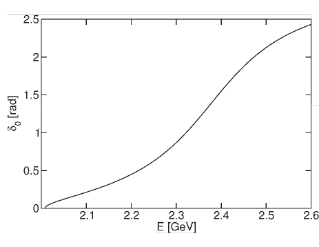
Figure 1: Phase of the $D\pi$ scalar form factor as a function of the c.m. energy $E=\sqrt{t}$.

In practice, if the ratio $r_{F}/r_{f}$ is not known, one can reverse the argument and use (14) as a constraint on the residues, in terms of the coefficients $a_{k}$ determined from fits to semileptonic decay data. However, the correlation is expected to be small, due to the fact that, as shown in Appendix A, in cases of interest the point $z_{p}\equiv z_{p}^{\rm I}$ is close to the boundary $|z|=1$. Therefore, the value of the new sum rule in this case is of more formal than phenomenological significance.

Of more practical value turns out to be another consequence of unitarity that is valid on the unitarity cut below the first inelastic threshold. By dividing both sides of (29) by the product $f^{*}\!f$, one has

$$\frac{1}{f^{*}(t)}-\frac{1}{f(t)}=2i\rho(t)\,,$$ (42)

which implies

$$\text{Im}\,\left[\frac{1}{f(t)}\right]=-\rho(t)\,.$$ (43)

The solution of this equation is

$$f(t)=\frac{1}{\psi(t)-i\rho(t)}\,,$$ (44)

where the undetermined function $\psi(t)$ is real on the elastic part of the unitarity cut, $t_{+}\leq t\leq t_{\text{in}}$. If a narrow resonance of mass $M$ and width $\Gamma$ is present, this function can be parametrized as

$$\psi(t)\sim\frac{M^{2}-t}{M\Gamma}\,,$$ (45)

up to factors holomorphic in a region $t_{+}<t<t_{\text{in}}$, where $t_{\text{in}}$ denotes the first inelastic threshold. By including all these factors in an energy-dependent $\Gamma(t)$, we can write, with a good approximation, the phase of the form factor in a limited energy region above the threshold as:

$$\arg[F(t)]=\arctan\left[\frac{M\Gamma(t)}{M^{2}-t}\right]\,.$$ (46)

This relation can be generalized to the case where overlapping resonances occur. In such a case, it is a well-known feature of $S$-matrix theory that simply summing Breit-Wigner resonances does not preserve unitarity, and the proper treatment would require allowing $\Gamma$ not only to be dependent on energy, but also a matrix-valued quantity over the various channels.

In Fig. 1 we show the phase $\delta_{0}$ of the scalar $D\pi$ form factor obtained from (46), using the standard Breit-Wigner expression $\Gamma(t)=\Gamma\rho(t)/\rho(M^{2})$, with the mass $M=2.351\,\text{GeV}$ and width $\Gamma=0.230\,\text{GeV}$ of the $D_{0}^{*}$ resonance [44]. We can assume that this value of the phase is a good approximation in the elastic region, below the opening of inelastic channels.

As discussed in the previous section, this additional information leads to a stronger constraint in the semileptonic region, given by Eq. (19). This constraint can be easily derived by solving the integral equation (21) for the function $\lambda(\theta)$ and using this solution in (19). For illustration, we present below the result of this analysis for the scalar $D\pi$ form factor. We take the value $\chi^{L}_{V}(q^{2}=0)=0.016$ from Ref. [25] and the outer function from Refs. [25, 27]:

$$\phi(z) = \frac{\sqrt{3}}{32\sqrt{\chi^{L}_{V}(0)}\sqrt{\pi}}\frac{m_{D}-m_{\pi}}{m_{D}+m_{\pi}}(1-z)(1+z)^{3/2}$$ (47)

$$\times\frac{(1-zz_{-})^{1/2}}{(1+z_{-})^{1/2}}\,,$$

where we take for simplicity $t_{0}=0$ in (7) and use the notation $z_{-}\equiv\tilde{z}(t_{-};0)$.

Taking for illustration $K=5$, we obtain the allowed domain for the coefficients $a_{k}$, $k\leq 4$:

$$1.78\,a_{0}^{2}+1.28\,a_{1}^{2}+1.13\,a_{2}^{2}+1.84\,a_{3}^{2}+2.33\,a_{4}^{2}$$ (48)

$$+ 0.79\,a_{0}a_{1}-0.49\,a_{0}a_{2}-1.61\,a_{0}a_{3}-1.96\,a_{0}a_{4}$$

$$- 0.13\,a_{1}a_{2}-0.84\,a_{1}a_{3}-1.09\,a_{1}a_{4}$$

$$+ 0.49\,a_{2}a_{3}+0.54\,a_{2}a_{4}+2.09\,a_{3}a_{4}\ \leq\ 1.$$

In this calculation, we assume that the phase is given up to the first inelastic threshold $t_{\text{in}}=(2.42\,\text{GeV})^{2}$ due to the $D\eta$ channel. The results are actually quite stable against the variation of $t_{\text{in}}$ around this value.

It is easy to see that the constraint (48) is stronger than the standard condition (17). In a typical application to semileptonic processes, the lowest coefficients $a_{k}$ are determined from fits of the data, and the aim is to set a bound on the next coefficient, which gives an estimate of the truncation error. In practical applications (see for instance [24]), the optimal values of the parameters are usually small, far from saturating the upper bound (17). To simulate such a situation, we take, for instance, the input values $a_{0}=0.10,\,a_{1}=0.08,\,a_{2}=0.07$ and $a_{3}=0.05$, for which the left hand side of (17) is 0.024. With this input, we obtain the constraint $|a_{4}|\leq 0.99$ from the standard inequality (17), and the smaller range $-0.62\leq a_{4}\leq 0.68$ from the improved constraint (48). We can then obtain a bound on the truncation error $\delta F(t_{-})$ at the end $t_{-}$ (corresponding to $z_{-}$) of the semileptonic region. From the parametrization (12), one can write this error as:

$$\delta F(t_{-})\approx\frac{|a_{4}|z_{-}^{4}}{|\phi(z_{-})|}\,.$$ (49)

Using the above limits on $a_{4}$ and the values $z_{-}=0.325$ and $\phi(z_{-})=0.176$ in our case, we obtain from (49) the uncertainties $\delta F(t_{-})\approx 0.063$ using the standard constraint (17) and $\delta F(t_{-})\approx 0.043$ using the improved constraint (48), which amounts to an improvement by about 30%. Similar results are obtained for a large class of input values for the lowest coefficients.

One can use also the optimal value of $t_{0}$ discussed in Sec. II, for which the semileptonic region is mapped onto a symmetric range in the $z$ plane. From Eq. (56), we obtain in our case $t_{0}=1.97\,\text{GeV}^{2}$ and $z_{-}=0.167$. Due to the smaller $z_{-}$, the error estimated from (49) is much smaller, but the constraints on the coefficient $a_{4}$ are similar to those reported above. In this case too, the improvement brought by the incorporation of the phase $\delta_{0}$ turns out to be quite important.

IV Summary and conclusions

In this paper we have continued the discussion of the effect of above-threshold singularities on model-independent form-factor parametrizations, initiated in Ref. [36]. We emphasized the fact that the presence of above-threshold poles does not affect the strength of the original model-independent constraints. By exploiting the connection between the first and the second Riemann sheets of a generic semileptonic form factor, we have derived a relation between the value of the form factor on the first Riemann sheet at the point $t_{p}$ that is the image of the location of the resonance pole on the unphysical (second) Riemann sheet, and the residues of the form factor and of the related elastic scattering amplitude. Using this expression in the combined constraint (14) involving the coefficients $a_{n}$ of a Taylor series expansion in the variable $z$ and the values of the form factor at the two complex-conjugate points, we derived a new sum rule relating the parametrization in the semileptonic region to the residues of the second-sheet poles of the form factor $F$ and the corresponding elastic scattering amplitude $f$. We argued however that the effect of this additional information in improving the model-independent constraints is expected to be small. Finally, we showed that from the mass and width of a narrow resonance, one can approximately obtain the phase of the form factor on a limited part of the unitarity cut. By including this additional information in the extremal problem, one obtains stronger constraints, given in (19), on the form-factor parametrization in the semileptonic region. This second method appears to be of more immediate utility in phenomenological applications.

Acknowledgments

I.C. acknowledges support from the Ministry of Research and Innovation, Contract PN 16420101/2016. B.G. was supported by the U.S. Department of Energy under Grant DE-SC0009919. R.F.L. was supported by the U.S. National Science Foundation under Grant No. 1403891.

Appendix A Uniformization of the two-sheet Riemann surface by $z$ mapping

In this Appendix we discuss the connection between the canonical variable $z$ in Eq. (7) used for solving the extremal problem in Sec. II and the Riemann structure of the elastic cut of the semileptonic form factor $F(t)$. We first note that (7) can be written as

$$z\equiv\tilde{z}(t;t_{0})=\frac{\sqrt{t_{+}-t_{0}}+ik(t)}{\sqrt{t_{+}-t_{0}}-ik(t)},$$ (50)

in terms of the function

$$k(t)=\sqrt{t-t_{+}}\,.$$ (51)

We recall that the first Riemann sheet is defined by $\arg(t-t_{+})\in(0,2\pi)$, while the second sheet is defined by $\arg(t-t_{+})\in(2\pi,4\pi)$. It follows that the first Riemann sheet corresponds to $\arg k(t)\in(0,\pi)$, which implies $k_{I}(t)>0$, and the second Riemann sheet corresponds to $\arg k(t)\in(\pi,2\pi)$, which implies $k_{I}(t)<0$, where $k_{I}(t)$ is the imaginary part of $k(t)$. Denoting by $k_{R}(t)$ the real part of $k(t)$, we obtain from (50):

$$|z|^{2}=\frac{[\sqrt{t_{+}-t_{0}}-k_{I}(t)]^{2}+k^{2}_{R}(t)}{[\sqrt{t_{+}-t_{0}}+k_{I}(t)]^{2}+k^{2}_{R}(t)}\,.$$ (52)

From this relation it follows that

$$k_{I}(t)>0\quad\Rightarrow\quad|z|<1,$$

$$k_{I}(t)<0\quad\Rightarrow\quad|z|>1.$$ (53)

Therefore, the first Riemann sheet of the $t$ plane, where $k_{I}(t)>0$, is mapped inside the unit circle in the $z$ plane, while the second sheet, where $k_{I}(t)<0$, is mapped outside the unit circle. In standard terminology, the variable (7) achieves the uniformization of the Riemann surface of the elastic cut, i.e., it maps the two Riemann sheets onto a single plane.

For the discussion in Sec. III, it is useful to have a relation between the images in the $z$ plane of the pole on the second sheet, and of the corresponding complex point situated on the first sheet. This relation follows from the symmetry property

$$\tilde{t}(z;t_{0})=\tilde{t}(z^{-1};t_{0})\,,$$ (54)

satisfied by (9), which shows that the images in the $z$ plane of the first-sheet and second-sheet points corresponding to the same complex $t$ value are inverse to each other,

$$z_{p}^{\rm I}=\frac{1}{z_{p}^{\rm II}}\,.$$ (55)

For a numerical illustration, we take for definiteness

$$t_{0}=t_{+}\left[1-\sqrt{1-\frac{t_{-}}{t_{+}}}\right]\,,$$ (56)

to achieve a symmetric semileptonic range ($-z_{\rm max}$, $z_{\rm max}$), as discussed in Sec. II. Then, using the masses and widths from [44] for the poles associated with the first vector resonances $K^{*}(892)$ and $D^{*}(2010)$ for the $K\pi$ and $D\pi$ vector form factors, respectively, we obtain from (50) the positions in the $z$ plane of $z_{p}^{\rm II}$ and their first-sheet counterparts $z_{p}^{\rm I}$. They read:

$$z_{p}^{\rm II}=-0.11\mp 1.05\,i,\quad\quad|z_{p}^{\rm II}|=1.06\,,$$ (57)

$$z_{p}^{\rm I}=-0.10\pm 0.94\,i,\quad\quad|z_{p}^{\rm I}|=0.95\,,$$

and

$$z_{p}^{\rm II}=0.978\mp 0.212\,i,\quad\quad|z_{p}^{\rm II}|=1.001\,,$$ (58)

$$z_{p}^{\rm I}=0.977\pm 0.212\,i,\quad\quad|z_{p}^{\rm I}|=0.999\,,$$

respectively. For the scalar resonance $D^{*}_{0}(2400)$ relevant to the scalar $D\pi$ form factor, the corresponding points are

$$z_{p}^{\rm II}=0.151\mp 1.179\,i,\quad\quad|z_{p}^{\rm II}|=1.19\,,$$ (59)

$$z_{p}^{\rm I}=0.107\pm 0.834\,i,\quad\quad|z_{p}^{\rm I}|=0.84\,.$$

We emphasize that the form factors have poles at the points $z_{p}^{\rm II}$, but are regular at $z_{p}^{\rm I}$.

References

- [1] N.N. Meiman, “Analytic expressions for upper limits of coupling constants in quantum field theory,” Zh. Eksp. Teor. Fiz. 44, 1228 (1963) [Sov. Phys. JETP 17, 830 (1963)].
- [2] S. Okubo, “Exact bounds for decay parameters,” Phys. Rev. D 3, 2807 (1971).
- [3] S. Okubo, “New improved bounds for parameters,” Phys. Rev. D 4, 725 (1971).
- [4] C. Bourrely, B. Machet, and E. de Rafael, “Semileptonic decays of pseudoscalar particles () and short distance behavior of quantum chromodynamics,” Nucl. Phys. B 189, 157 (1981).
- [5] P.L. Duren, Theory of Spaces, Academic Press, New York, 1970.
- [6] M.G. Krein and P.I. Nudelman, “On some new problems for functions of Hardy class and continual families of functions with double orthogonality,” Sov. Math. Dokl. 14, 435 (1973) [Dokl. Acad. Nauk. SSSR 209, 537 (1973)].
- [7] E. de Rafael and J. Taron, “Constraints on heavy meson form-factors,” Phys. Lett. B 282, 215 (1992).
- [8] C.E. Carlson, J. Milana, N. Isgur, T. Mannel, and W. Roberts, “Comment regarding bounds upon heavy meson form-factors,” Phys. Lett. B 299, 133 (1993).
- [9] A.F. Falk, M.E. Luke, and M.B. Wise, “Analyticity and the Isgur-Wise function,” Phys. Lett. B 299, 123 (1993).
- [10] J.G. Körner, D. Pirjol, and C. Dominguez, “Analyticity bounds on the Isgur-Wise function,” Phys. Lett. B 301, 257 (1993).
- [11] B. Grinstein and P.F. Mende, “On constraints for heavy meson form-factors,” Phys. Lett. B 299, 127 (1993) [hep-ph/9211216].
- [12] I. Caprini, “Effect of upsilon poles on the analyticity constraints for heavy meson form-factors,” Z. Phys. C 61, 651 (1994).
- [13] I. Caprini, “Slope of the Isgur-Wise function from a QSSR constraint on the couplings,” Phys. Lett. B 339, 187 (1994) [hep-ph/9408238].
- [14] C.G. Boyd, B. Grinstein, and R.F. Lebed, “Constraints on form-factors for exclusive semileptonic heavy to light meson decays,” Phys. Rev. Lett. 74, 4603 (1995) [hep-ph/9412324].
- [15] C.G. Boyd, B. Grinstein, and R.F. Lebed, “Model independent determinations of , form-factors,” Nucl. Phys. B 461, 493 (1996) [hep-ph/9508211].
- [16] C.G. Boyd and M.J. Savage, “Analyticity, shapes of semileptonic form-factors, and ,” Phys. Rev. D 56, 303 (1997) [hep-ph/9702300].
- [17] C.G. Boyd, B. Grinstein, and R.F. Lebed, “Precision corrections to dispersive bounds on form-factors,” Phys. Rev. D 56, 6895 (1997) [hep-ph/9705252].
- [18] L. Lellouch, “Lattice constrained unitarity bounds for decays,” Nucl. Phys. B 479, 353 (1996) [hep-ph/9509358].
- [19] I. Caprini, L. Lellouch, and M. Neubert, “Dispersive bounds on the shape of form-factors,” Nucl. Phys. B 530, 153 (1998) [hep-ph/9712417].
- [20] I. Caprini, “Dispersive and chiral symmetry constraints on the light meson form-factors,” Eur. Phys. J. C 13, 471 (2000) [hep-ph/9907227].
- [21] C. Bourrely and I. Caprini, “Bounds on the slope and the curvature of the scalar form-factor at zero momentum transfer,” Nucl. Phys. B 722, 149 (2005) [hep-ph/0504016].
- [22] R.J. Hill, “Constraints on the form factors for and implications for ,” Phys. Rev. D 74, 096006 (2006) [hep-ph/0607108].
- [23] T. Becher and R.J. Hill, “Comment on form-factor shape and extraction of from ,” Phys. Lett. B 633, 61 (2006) [hep-ph/0509090].
- [24] C. Bourrely, I. Caprini, and L. Lellouch, “Model-independent description of decays and a determination of ,” Phys. Rev. D 79, 013008 (2009) [Erratum: Phys. Rev. D 82, 099902 (2010)] [arXiv:0807.2722 [hep-ph]].
- [25] B. Ananthanarayan, I. Caprini, and I. Sentitemsu Imsong, “Implications of unitarity and analyticity for the form factors,” Eur. Phys. J. A 47, 147 (2011) [arXiv:1108.0284 [hep-ph]].
- [26] G. Abbas, B. Ananthanarayan, I. Caprini, and I. Sentitemsu Imsong, “Improving the phenomenology of form factors with analyticity and unitarity,” Phys. Rev. D 82, 094018 (2010) [arXiv:1008.0925 [hep-ph]].
- [27] G. Abbas, B. Ananthanarayan, I. Caprini, I. Sentitemsu Imsong, and S. Ramanan, “Theory of unitarity bounds and low energy form factors,” Eur. Phys. J. A 45, 389 (2010) [arXiv:1004.4257 [hep-ph]].
- [28] B. Ananthanarayan, I. Caprini, and I. Sentitemsu Imsong, “Implications of the recent high statistics determination of the pion electromagnetic form factor in the timelike region,” Phys. Rev. D 83, 096002 (2011) [arXiv:1102.3299 [hep-ph]].
- [29] B. Ananthanarayan, I. Caprini, and I. Sentitemsu Imsong, “Spacelike pion form factor from analytic continuation and the onset of perturbative QCD,” Phys. Rev. D 85, 096006 (2012) [arXiv:1203.5398 [hep-ph]].
- [30] B. Ananthanarayan, I. Caprini, D. Das, and I. Sentitemsu Imsong, “Two-pion low-energy contribution to the muon with improved precision from analyticity and unitarity,” Phys. Rev. D 89, 036007 (2014) [arXiv:1312.5849 [hep-ph]].
- [31] B. Ananthanarayan, I. Caprini, D. Das, and I. Sentitemsu Imsong, “Precise determination of the low-energy hadronic contribution to the muon from analyticity and unitarity: An improved analysis,” Phys. Rev. D 93, 116007 (2016) [arXiv:1605.00202 [hep-ph]].
- [32] R.J. Hill and G. Paz, “Model independent extraction of the proton charge radius from electron scattering,” Phys. Rev. D 82, 113005 (2010) [arXiv:1008.4619 [hep-ph]].
- [33] B. Ananthanarayan, I. Caprini, and B. Kubis, “Constraints on the form factor from analyticity and unitarity,” Eur. Phys. J. C 74, 3209 (2014) [arXiv:1410.6276 [hep-ph]].
- [34] I. Caprini, “Testing the consistency of the transition form factor with unitarity and analyticity,” Phys. Rev. D 92, 014014 (2015) [arXiv:1505.05282 [hep-ph]].
- [35] C.G. Boyd and R.F. Lebed, “Improved QCD form-factor constraints and ,” Nucl. Phys. B 485, 275 (1997) [hep-ph/9512363].
- [36] B. Grinstein and R.F. Lebed, “Above-Threshold Poles in Model-Independent Form Factor Parametrizations,” Phys. Rev. D 92, 116001 (2015) [arXiv:1509.04847 [hep-ph]].
- [37] R.E. Peierls, “Interpretation and properties of propagators,” in Proceedings of the 1954 Glasgow Conference on Nuclear and Meson Physics, edited by E.H. Bellamy and R.G. Moorhouse (Pergamon Press, New York, 1955).
- [38] G. Barton, Introduction to Dispersion Techniques in Field Theory, W.A. Benjamin, New York, Amsterdam, 1965.
- [39] E. Fermi, “Lectures on pions and nucleons,” Nuovo Cim. 2, 17 (1955) [Riv. Nuovo Cim. 31, 1 (2008)].
- [40] K.M. Watson, “Some general relations between the photoproduction and scattering of mesons,” Phys. Rev. 95, 228 (1954).
- [41] S.M. Roy, “Exact integral equation for pion pion scattering involving only physical region partial waves,” Phys. Lett. 36B, 353 (1971).
- [42] M. Micu, “Improved optimal bounds using the Watson theorem,” Phys. Rev. D 7, 2136 (1973).
- [43] I. Caprini, G. Colangelo, and H. Leutwyler, “Mass and width of the lowest resonance in QCD,” Phys. Rev. Lett. 96, 132001 (2006) [hep-ph/0512364].
- [44] C. Patrignani et al. [Particle Data Group Collaboration], “Review of Particle Physics,” Chin. Phys. C 40, 100001 (2016).