Search for astrophysical sources of neutrinos using cascade events in IceCube

Abstract

The IceCube neutrino observatory has established the existence of a flux of high-energy astrophysical neutrinos inconsistent with the expectation from atmospheric backgrounds at a significance greater than $5\sigma$. This flux has been observed in analyses of both track events from muon neutrino interactions and cascade events from interactions of all neutrino flavors. Searches for astrophysical neutrino sources have focused on track events due to the significantly better angular resolution of track reconstructions. To date, no such sources have been confirmed. Here we present the first search for astrophysical neutrino sources using cascades interacting in IceCube with deposited energies as small as 1 TeV. No significant clustering was observed in a selection of 263 cascades collected from May 2010 to May 2012. We show that compared to the classic approach using tracks, this statistically-independent search offers improved sensitivity to sources in the southern sky, especially if the emission is spatially extended or follows a soft energy spectrum. This enhancement is due to the low background from atmospheric neutrinos forming cascade events and the additional veto of atmospheric neutrinos at declinations $\lesssim-30^{\circ}$.

1 Introduction

Neutrinos are promising messenger particles for astrophysical observations due to their extremely small interaction cross-sections and lack of electric charge. They can travel enormous distances largely unimpeded by intervening matter and undeflected by magnetic fields. These properties make it possible to associate neutrinos from distant sources with each other and with known sources of electromagnetic radiation. Furthermore, because neutrinos are produced in high-energy hadronic interactions, observations of astrophysical neutrinos will shed light on the still-elusive origins of the highest-energy cosmic rays (Gaisser et al., 1995; Learned & Mannheim, 2000; Becker, 2008).

IceCube is the first $\mathrm{km^{3}}$-scale neutrino detector (Achterberg et al., 2006). Using an array of photomultiplier tubes (PMTs) deployed deep in the antarctic glacial ice near the South Pole, it can detect neutrinos of all flavors by collecting the Cherenkov light emitted by the relativistic charged particles produced when neutrinos interact with atomic nuclei in the ice. Neutrinos produce one of two topologically distinct signatures: tracks and cascades. Charged current (CC) muon neutrino interactions yield long-lived muons that can travel several kilometers through the ice (Chirkin & Rhode, 2004), producing an elongated track signature in the detector. Charged current interactions of other neutrino flavors, and all neutral current (NC) interactions, yield hadronic and electromagnetic showers that typically range less than $20\,\mathrm{m}$ (Aartsen et al., 2014a), with 90% of the light emitted within $4\,\mathrm{m}$ of the shower maximum (Radel & Wiebusch, 2013) — a short distance compared to the scattering and absorption lengths of light in the ice (Aartsen et al., 2013b) as well as the spacing of the PMTs. These showers produce a nearly spherically symmetric cascade signature in light.

A flux of astrophysical neutrinos above $\sim 60\,\mathrm{TeV}$ inconsistent with the expectation from atmospheric backgrounds at greater than $5\sigma$ was first established using neutrinos interacting within the instrumented volume of IceCube (Aartsen et al., 2014c, 2015a). The majority of events contributing to this measurement were cascades. More recently, this flux has been confirmed in an analysis of tracks from muon neutrinos above $\sim 300\,\mathrm{TeV}$ originating in the northern sky (Aartsen et al., 2015c, 2016c). No significant anisotropy has yet been observed, and the neutrino flavor ratio at Earth is consistent with 1:1:1 (Aartsen et al., 2015d).

Searches for astrophysical neutrino sources have traditionally focused on track events because the elongated signature gives much better angular resolution than can be obtained for cascades. While ANTARES recently reported the addition of a cascade selection to their all-sky search for sources of steady neutrino emission (Adrian-Martinez et al., 2015), IceCube has so far excluded cascades from its all-sky search (Aartsen et al., 2017a) except in the simplified analysis applied only to very high-energy contained events (Aartsen et al., 2015a).

In this paper, we present the first all-sky search for astrophysical neutrino sources producing cascades in IceCube with deposited energies as small as 1 TeV. This analysis includes 263 cascades observed from May 2010 to May 2012. We find that, due to the relatively low rate of atmospheric backgrounds in this sample, this search reduces the energy threshold in the southern sky relative to previous IceCube work with tracks. The sensitivity of this search is much less dependent on the declination, spatial extension, and emission spectrum of a possible source. In the following sections, we begin with an overview of the detector, experimental dataset, and statistical methods used in this analysis before reporting results from the two-year sample and discussing directions for future work.

2 IceCube

The IceCube detector (described in detail in Aartsen et al. (2017b)) consists of 5160 Digital Optical Modules (DOMs) buried in the glacial ice near the South Pole. The DOMs are mounted on 86 vertical “strings”, with 60 DOMs on each string. Each string is connected to a central lab on the surface by a cable that provides power and communication with the data acquisition (DAQ) system (Abbasi et al., 2009). Seventy-eight of the strings are arranged in a hexagonal grid with a spacing of 125 m; on these strings, DOMs are distributed uniformly from 1450 m to 2450 m below the surface of the ice. The remaining 8 strings make up the denser DeepCore in-fill array (Abbasi et al., 2012), with inter-string spacing of 30 to 60 m. The in-fill strings include 50 DOMs in the particularly clear ice at depths of 2100 m to 2450 m and an additional 10 DOMs evenly spaced at depths of 1750 m to 1850 m. Construction was performed during Austral summers starting in 2004. A nearly complete 79-string configuration began taking data in May 2010, and the first year of data from the complete 86-string detector was taken from May 2011 to May 2012.

Each DOM includes a 25 cm diameter PMT (Abbasi et al., 2010) and supporting electronics. A local coincidence condition occurs when a DOM and one of its nearest neighbors exceed a threshold of 1/4 of the mean expected voltage from a single photoelectron (PE). When at least eight DOMs observe local coincidence within $6.4\,\mathrm{\mu s}$, the DAQ produces an event consisting of 400 ns digitized waveforms from all DOMs observing local coincidence and 75 ns waveforms from all other DOMs exceeding the threshold. The waveforms are then decomposed into series of pulse arrival times and PE counts which are used to reconstruct the trajectory and deposited energy of the relativistic particles in the detector (Ahrens et al., 2004; Aartsen et al., 2014a).

The simple eight-DOM trigger accepts neutrino-induced events with very high efficiency. Unfortunately, even deep in the glacial ice, cosmic ray-induced atmospheric muons trigger the detector at an average rate of 2.7 kHz, overwhelming the trigger rate of atmospheric neutrinos ($\sim 20\,\mathrm{mHz}$) and rare astrophysical neutrinos. An initial data reduction step performed at the South Pole reduces the event rate by a factor of 100 by rejecting lower-energy events that are consistent with downgoing tracks. The remaining dataset, still dominated by downgoing muons, is transmitted to the northern hemisphere via satellite for further analysis.

3 Neutrino Selection

IceCube searches for moderate to high energy neutrinos generally exploit one of two methods to reject the atmospheric muon background. The largest effective volume and best angular resolution are available when incoming muon tracks are accepted. This approach offers good performance for muon neutrinos from the northern celestial hemisphere because only neutrinos can survive passage through the intervening earth before producing upgoing muons in the ice. However, neutrino- and cosmic ray-induced downgoing muon tracks entering the detector from above produce nearly indistinguishable event topologies. Astrophysical neutrinos from the southern sky can be identified on a statistical basis if the neutrino spectrum is harder than the atmospheric muon spectrum, but this strategy increases the energy threshold to $\sim 100\,\mathrm{TeV}$ in the southern sky, compared to only $\sim 1\,\mathrm{TeV}$ in the northern sky (Aartsen et al., 2014d).

An alternative method is to restrict the analysis to “starting events”, for which the earliest observed pulses occur within the instrumented volume. The use of the outermost DOMs as a veto layer allows the rejection of atmospheric muons that enter the detector from above or merely pass sufficiently close to the instrumented volume to produce a signal capable of surviving the initial filter. Analyses of starting events are able to accept neutrinos of all flavors and interaction types because only neutrinos can pass undetected through the veto layer before interacting in the ice. Veto methods currently used in IceCube analyses significantly reduce the effective volume for detecting $\nu_{\mu}$-induced muon tracks, resulting in a smaller final sample that is dominated by cascades. The angular uncertainty of cascade reconstructions ($\gtrsim 10^{\circ}$) is large compared to that of track reconstructions ($\lesssim 1^{\circ}$). However, the requirement that the neutrino interaction vertex is located within the instrumented volume results in good energy resolution (within $\sim 10\%$) (Aartsen et al., 2014a) compared to incoming muon tracks originating at an unknown distance from the detector.

Lower energy muons not only deposit less energy overall, but they may travel larger distances between substantial energy losses due to the stochastic nature of radiative processes at these energies. The initial discovery of astrophysical neutrinos used only the outermost DOMs as a veto layer and thus achieved adequate background rejection only at energies $\gtrsim 60\,\mathrm{TeV}$ (Aartsen et al., 2014c). In a follow-up analysis, the energy threshold was reduced to $\sim 1\,\mathrm{TeV}$ by scaling the veto thickness as a function of total collected charge (Aartsen et al., 2015b) such that events depositing as little as 100 PE could be observed, provided that the earliest light was found in the DeepCore in-fill array.

This adaptive veto event selection was applied to two years of data taken from May 2010 to May 2012 — one year using the nearly-complete 79-string configuration and one year using the complete 86-string detector. In a total of 641 days of IceCube livetime, 283 cascade and 105 track events were found (Aartsen et al., 2015b). While most of the track events are accepted by $\nu_{\mu}$ point source searches (Aartsen et al., 2014d) and a small fraction of the cascades are included in the earlier high energy starting event analysis (Aartsen et al., 2013a, 2014c), the majority of these cascades have not yet been studied in the context of spatial clustering. In this paper, we turn our attention to 263 of these cascades with deposited energies of $1\,\mathrm{TeV}-1\,\mathrm{PeV}$ to perform an astrophysical neutrino source search that is complementary to and statistically independent from traditional track analyses.

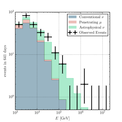
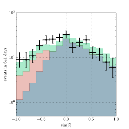
Figure 1: Reconstructed energy (left) and declination (right) distributions for the best-fit atmospheric and astrophysical spectra (shaded histograms) obtained in Aartsen et al. (2015b) compared to the distributions for the 263 cascades (black crosses) depositing at least $1\,\mathrm{TeV}$ observed in that analysis. Atmospheric muons misidentified as cascades after passing undetected through the veto layer are concentrated at $\sin(\delta)<-0.3$, while in the same range some atmospheric neutrinos are rejected because they are accompanied by incoming muons.

The reconstructed energy and declination distributions for the 263 observed cascades are compared in Figure 1 with the expectation from the best-fit atmospheric and astrophysical fluxes found in the spectral analysis. The fitted astrophysical component follows an $E^{-2.46}$ spectrum and contributes an expected $71^{+9.5}_{-8.4}$ cascades in 641 days — a far larger fraction of the total event rate than in previous source searches with tracks (Aartsen et al., 2017a). The neutrino energy distribution is shown in Figure 2 for the best-fit spectrum as well as the hard ($E^{-2}$) and soft ($E^{-3}$) source spectrum hypotheses tested directly in this paper. For an $E^{-3}$ spectrum, we expect 90% of events to have energies between 2 TeV and 90 TeV; for an $E^{-2}$ spectrum this range shifts to $6\,\mathrm{TeV}-5\,\mathrm{PeV}$.

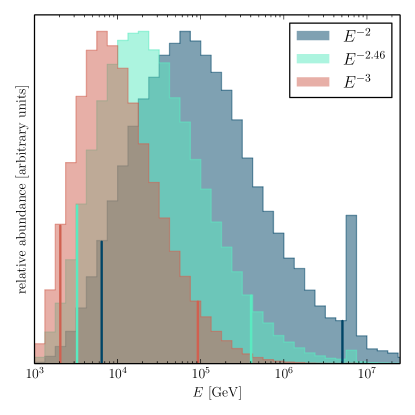
Figure 2: Neutrino energy distributions expected from sources emitting a hard ($E^{-2}$, blue) or soft ($E^{-3}$, red) spectrum compared with the best-fit all-sky astrophysical component following an $E^{-2.46}$ spectrum (green). Each distribution includes all standard model neutrino flavors, assuming a 1:1:1 flavor ratio at Earth with equal fluxes of $\nu$ and $\bar{\nu}$. Vertical lines indicate intervals containing 90% of events. While no such events have yet been observed, an enhanced acceptance is expected for $\nu_{e}$ at $6.3\,\mathrm{PeV}$ due to the Glashow resonance (Glashow, 1960).

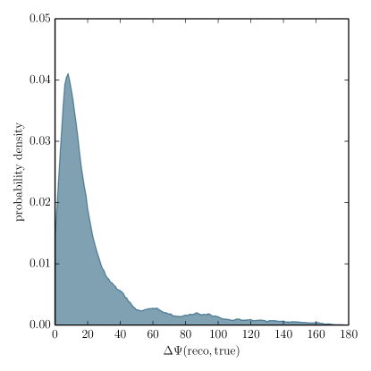
Figure 5: Expected distribution of angular separation between reconstructed and true neutrino direction for signal MC following an $E^{-2.46}$ spectrum. While the distribution includes a tail extending all the way to $180^{\circ}$, 50% (90%) of events are reconstructed within $13^{\circ}$ ($45^{\circ}$).

In this work, we use the same per-event reconstructions as in the spectral analysis. The strict containment requirement results in good energy resolution up to at least $\sim\text{few}\,\mathrm{PeV}$. The reconstructed energy agrees with the neutrino energy within $\sim 10\%$ for 68% of CC $\nu_{e}$ interactions and is on average proportional to neutrino energy for other interaction flavors (Aartsen et al., 2015b). Agreement between reconstructed and true neutrino energy is shown in Figure 3. The primary challenge for source searches with cascades is the angular reconstruction, for which the performance is shown as a function of energy in Figure 4 and averaged over all energies in Figure 5. At low energies, the reconstruction benefits to some degree from the preferential selection of interactions in or near the more densely instrumented DeepCore. At high energies, performance is somewhat poorer than optimal — compare with, e.g., Aartsen et al. (2014a) — likely due to the specific reconstruction settings used for this sample, which are less computationally intensive but which employ a coarser description of the expected light yield and a less rigorous scan of the directional likelihood landscape.

4 Methods and Performance

We use an unbinned maximum likelihood method to quantify the extent to which the observed events are more consistent with a spatially localized astrophysical signal hypothesis than a randomly distributed background hypothesis. This method exploits the spatial distribution of events as well as the distribution of per-event deposited energies, where the latter improves the sensitivity to sources with harder spectra than atmospheric backgrounds. While we largely follow the approach used in traditional track analyses (most recently Aartsen et al., 2017a), the specific signal and background models are modified to accommodate the large angular uncertainties and overall low statistics of the cascade event selection. In Section 4.1 we review the likelihood construction, including explanations for changes with respect to previous work with tracks. In Section 4.2 we introduce the specific hypothesis tests considered in this work. Systematic uncertainties are discussed in Section 4.3 and the performance of the cascade analysis is presented in Section 4.4.

4.1 Maximum Likelihood Method

The likelihood is expressed as a product over events $i$:

$$\mathcal{L}(n_{s},\gamma) =\prod_{i}{}\left[\frac{n_{s}}{N}{}\mathcal{S}_{i}{}+\left(1-\frac{n_{s}}{N}\right){}\mathcal{B}_{i}\right],$$ (1)

where $n_{s}$ is the number of signal events, $\gamma$ is the spectral index of the source, $N=263$ is the total number of events, $\mathcal{S}_{i}$ is the likelihood of event $i$ contributing to the source, and $\mathcal{B}_{i}$ is the likelihood of event $i$ contributing to atmospheric or unresolved astrophysical backgrounds. $\mathcal{S}_{i}$ depends on the properties of both event $i$ and the source hypothesis (including spectral index $\gamma$), while $\mathcal{B}_{i}$ depends only on the properties of the events. $\hat{n}_{s}$ and $\hat{\gamma}$ are the values that give the maximum likelihood $\hat{\mathcal{L}}$, subject to the constraint that $\hat{n}_{s}\geq 0$. Events that are more correlated spatially or energetically with the source hypothesis obtain larger values for $\mathcal{S}_{i}$, driving the fit towards larger values of $\hat{n}_{s}$ and $\hat{\mathcal{L}}$.

We approximate the signal and background likelihoods $\mathcal{S}_{i}$ and $\mathcal{B}_{i}$ as products of space and energy factors: $S_{i}^{\text{space}}\cdot S_{i}^{\text{energy}}$ and $B_{i}^{\text{space}}\cdot B_{i}^{\text{energy}}$, respectively. Each factor is obtained by convolving the properties of the event origin — either astrophysical source, or atmospheric or unresolved astrophysical background — first with the detector response and then with the event reconstruction resolution. For $B_{i}^{\text{space}}$, this is done using a normalized histogram of reconstructed declination $\delta$ for an ensemble of background-like events, accounting for detector effects and smearing from finite angular resolution simultaneously. Similarly, for $S_{i}^{\text{energy}}$ and $B_{i}^{\text{energy}}$, we use normalized histograms of the logarithm of the deposited energy $\log_{10}E$ for ensembles of signal-like and background-like events, respectively, accounting for the declination dependence with separately-normalized histograms in each of ten bins in $\sin\delta$. $S_{i}^{\text{energy}}$ is computed from signal Monte Carlo (MC) on a grid of spectral indices $\gamma$ ranging from 1 to 4. For a given event, $B_{i}^{\text{space}}$, $S_{i}^{\text{energy}}$ and $B_{i}^{\text{energy}}$ are equal to the values of the histograms for the bin containing the event. The location of IceCube at the geographic South Pole allows us to express these factors as functions of declination, rather than zenith angle with respect to the detector, without loss of information. A small additional dependence on azimuth angle is neglected.

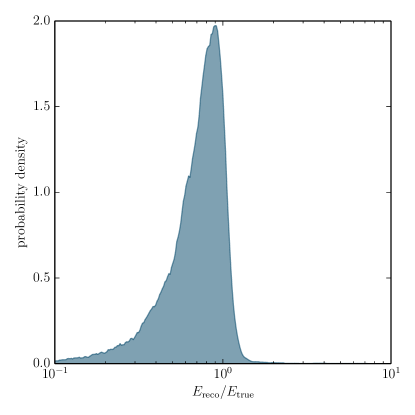
Figure 3: Ratio of reconstructed to true neutrino energy for signal MC following an $E^{-2.46}$ spectrum. Reconstructed energy is on average proportional to true neutrino energy for all interaction flavors, with agreement within $\sim 10\%$ for 68% of CC $\nu_{e}$ interactions.

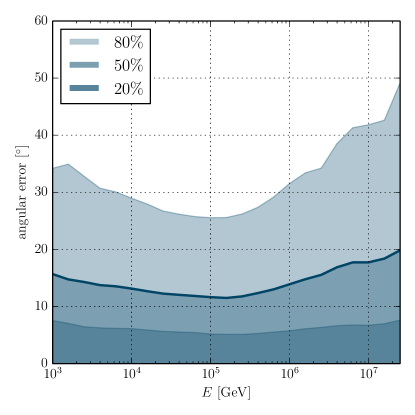
Figure 4: Expected angular reconstruction performance as a function of neutrino energy. Shaded regions indicate the radii of error circles covering 20%, 50%, and 80% of events. Below $20\,\mathrm{PeV}$, the median angular error, highlighted by the dark blue curve, ranges from $11^{\circ}$ to $20^{\circ}$.

In the classic track analysis, the background per-event likelihoods are constructed from the full experimental dataset. With a large sample of well-reconstructed muon tracks dominated by atmospheric backgrounds, both $B_{i}^{\text{space}}$ and $B_{i}^{\text{energy}}$ are well constrained statistically even for dense binning in both $\sin\delta$ and $\log_{10}E$. By contrast, our sample of only 263 cascade events is only sufficient to constrain $B_{i}^{\text{space}}$. Thus our first modification to the method is to construct $B_{i}^{\text{energy}}$ from neutrino and atmospheric muon MC simulations weighted to the best-fit atmospheric and astrophysical spectra found by the all-sky flux analysis using these events (Aartsen et al., 2015b). In this way we obtain a detailed estimate of the energy distribution throughout the sky, even at energies not yet observed at all declinations in two years of experimental livetime.

The signal space factor $S_{i}^{\text{space}}$ is obtained by convolving a source hypothesis with an analytical estimate of the spatial probability density distribution for event $i$ originating at reconstructed right ascension and declination $(\alpha_{i},\delta_{i})$. In track analyses, it is a good approximation to model this distribution as a 2D Gaussian with width $\sigma_{i}$ estimated event-by-event using a dedicated reconstruction. We modify this treatment for cascades both because the angular uncertainties are much larger and because it is too computationally expensive to estimate them directly for each event.

In this analysis we parameterize the angular resolution as a function of reconstructed declination $\delta_{i}$ and energy $E_{i}$. In parts of this parameter space, either the declination or right ascension errors tend to be systematically larger, so these are treated independently. For each of 10 bins in $\sin\delta$ and 12 in $\log_{\text{10}}E$, we find the values $\sigma_{\alpha}$ and $\sigma_{\delta}$ such that $|\alpha_{i}-\alpha_{i}^{\text{true}}|<\sigma_{\alpha}$, and separately $|\delta_{i}-\delta_{i}^{\text{true}}|<\sigma_{\delta}$, for 68.27% of simulated events in the bin. The spatial probability density distribution for observed event $i$ is the product of 1D Gaussians with these widths, normalized such that the distribution integrates to unity on the sphere.

We consider two types of source hypothesis: point sources and the galactic plane — an extremely extended source. A point source is modeled as a 2D delta distribution centered at the source coordinates. The expected emission from the galactic plane is in general model-dependent. Here we represent the galactic plane as a simple line source at galactic latitude $b=0$. In either case, $S_{i}^{\text{space}}$ is obtained by convolving the source hypothesis with the per-event spatial probability density distributions described above. For point sources, the convolution is trivial; for the galactic plane, it is evaluated numerically on a grid with $1^{\circ}$ spacing.

4.2 Hypothesis Tests

In this work we consider three search categories: (1) a scan for point-like sources anywhere in the sky, (2) a search for neutrinos correlated with an a priori catalog of promising source candidates, and (3) a search for neutrinos correlated with the galactic plane. Each search entails multiple specific hypothesis tests. The all-sky scan tests for point-like sources on a dense grid of coordinates throughout the sky. The catalog search tests the coordinates of each source candidate individually. The galactic plane search includes partially correlated tests for a hypothesis including the entire galactic plane and a hypothesis including only the part of the galactic plane in southern sky.

The test statistic used to compute significances is the likelihood ratio:

$$\mathcal{T} =-2\ln\left[\frac{\mathcal{L}(n_{s}=0)}{\mathcal{L}(\hat{n}_{s},\hat{\gamma})}\right],$$ (2)

where $\mathcal{L}(n_{s}=0)$ is the background-only likelihood and is independent of $\gamma$. For an individual hypothesis, the pre-trials significance $p_{\text{pre}}$ of an observation yielding a test statistic $\mathcal{T}_{\text{obs}}$ is the probability of observing $\mathcal{T}>\mathcal{T}_{\text{obs}}$ if the background-only hypothesis were true. The background-only $\mathcal{T}$ distribution is found by performing the likelihood test on a large number of ensembles with randomized $\alpha_{i}$, which removes any clustering that may be present in the true event ensemble. At declinations close to the poles, $|\delta_{i}|>60^{\circ}$, randomizing $\alpha_{i}$ alone is insufficient to remove a possible cluster of cascades. This is addressed by additionally randomizing $\sin\delta_{i}$ for the 15 events within these regions.

The pre-trials results, $p_{\text{pre}}$, do not account for multiple and partially correlated hypothesis tests conducted in each search category. The post-trials significance is determined by the most significant $p_{\text{pre}}$ for any hypothesis in the category. Specifically, for each search category we find the post-trials probability $p_{\text{post}}$ of observing any $\min(p_{\text{pre}})<\min(p_{\text{pre}})_{\text{obs}}$ if the background-only hypothesis were true. The background-only $\min(p_{\text{pre}})$ distribution is found by generating additional randomized event ensembles and noting the most significant $p_{\text{pre}}$ in each one. This construction leads to one final significance $p_{\text{post}}$ for each type of search; a further look-elsewhere effect between the all-sky, source candidate catalog, and galactic plane searches is not explicitly accounted for. This method is conservative in that it strictly controls only the false positive, but not the true positive, error rate.

We use the classical statistical approach (Neyman, 1937; Lehmann & Romano, 2005) to calculate the sensitivity, discovery potential, and flux upper limits. The flux level is determined using randomized trials in which signal MC events are injected at a Poisson rate $n_{\text{sig}}$ and distributed according to the spatial and energetic properties of the signal hypothesis. The remaining $N-n_{\text{sig}}$ events are injected according to the background modeling procedure described above. The sensitivity flux is that which gives a 90% probability of obtaining $\mathcal{T}>\mathcal{T}_{\text{med}}$, where $\mathcal{T}_{\text{med}}$ is the median of the background-only $\mathcal{T}$ distribution. The discovery potential flux is obtained by the same procedure, but for a 50% probability of yielding a $5\sigma$ pre-trials significance. The 90% confidence level upper limit is the larger of either the sensitivity or that flux which gives a 90% probability of obtaining $\mathcal{T}>\mathcal{T}_{\text{obs}}$.

4.3 Systematic Uncertainties

The randomization procedures described in the previous section yield background models and significances that are robust against systematic uncertainties. However, flux calculations in this analysis are based on detailed neutrino signal MC as described in Aartsen et al. (2016c) and are subject to systematic uncertainties. We estimate the impact of these uncertainties on our results via their impact on the cascade angular resolution and signal acceptance. Of these, uncertainties related to the angular resolution are the dominant effect. Reconstruction performance estimates from the baseline MC are limited by statistical uncertainties in the observed light as well as any practical computational tradeoffs made in data processing. These estimates do not account for possible systematic errors in the modeling of light absorption and scattering in either the bulk of South Pole glacial ice or the narrow columns of refrozen ice surrounding the DOMs. Uncertainties in the light yield from showers and the optical efficiency of the DOMs are also neglected in the baseline MC. Taken together, we estimate that these effects introduce an angular resolution uncertainty that can be approximated as a Gaussian smearing of the baseline point spread function with width $\sigma_{\text{sys}}\sim 8^{\circ}$ (compare, e.g., the typical per-event errors in Aartsen et al. (2014c) with the median expected pure-statistical errors in Aartsen et al. (2014a)). Applying this smearing weakens the sensitivity by $\sim 20\%$ ($\sim 23\%$) for sources following an $E^{-2}$ ($E^{-3}$) spectrum, approximately independent of source declination.

The uncertainties described above also have a small impact on the estimated signal acceptance of the event selection. Uncertainties in the DOM efficiency are on average inversely correlated with uncertainties in the scattering and absorption coefficients, so we can safely estimate the impact of these uncertainties using a parameterization from available MC datasets which only vary the DOM efficiency explicitly. We consider a reduced DOM efficiency of $-10\%$ relative to the baseline MC, which decreases both the number of accepted events for a given flux and the reconstructed deposited energy of each simulated event. Under this change most signal events are assigned slightly smaller weights $(S/B)_{i}^{\text{energy}}$ and some fall below the detection threshold, weakening the sensitivity by $\sim 4\%$, approximately independent of source spectrum and declination.

The signal acceptance also depends on the neutrino interaction cross section, which is known within a similar uncertainty $+4\%/-2.4\%$ below 100 PeV (Cooper-Sarkar et al., 2011). The resulting impact on this analysis is in general dependent on declination and neutrino energy, as an increased (decreased) cross section would simultaneously increase (decrease) the probability of detecting a neutrino upon arrival in the instrumented volume but decrease (increase) the probability of a neutrino reaching the detector after passing through the intervening earth and ice. We take $\sim 4\%$ as a conservative estimate of the acceptance uncertainty due to neutrino interaction cross section uncertainties.

While the signal acceptance depends largely on the total amount of light recorded by the DOMs, the angular resolution depends most strongly on the spatial and temporal distribution of light in the detector. Therefore, we take these effects to be approximately independent and add the above values in quadrature to obtain a total systematic uncertainty of 21% (24%) for sources following an $E^{-2}$ ($E^{-3}$) spectrum. All following sensitivities, discovery potentials, and flux upper limits include this factor.

4.4 Performance

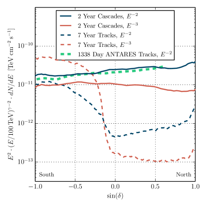
Figure 6: Per-flavor sensitivity of the present 2-year cascade analysis and previous 7-year IceCube (Aartsen et al., 2017a) and 1338-day ANTARES (Adrian-Martinez et al., 2014) track analyses as a function of declination for a hard spectrum ($\gamma=2$) and soft spectrum ($\gamma=3$).

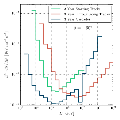
Figure 7: Per-flavor differential sensitivity for a source at $\delta=-60^{\circ}$ for track analyses of throughgoing (Aartsen et al., 2014d) and starting (Aartsen et al., 2016b) tracks, compared to this cascade analysis using the event selection from Aartsen et al. (2015b). The sensitivity in cascades is enhanced at $6.3\,\mathrm{PeV}$ due to the Glashow resonance (Glashow, 1960). In this plot, all sensitivities are calculated for an equal three year exposure.

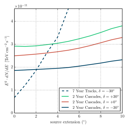
Figure 8: Per-flavor sensitivity as a function of angular extension of the source. For cascades, a point source hypothesis is used in the likelihood regardless of injected source extension. For tracks, the sensitivity is found for an extended source hypothesis matching the injected signal using the throughgoing track dataset from Aartsen et al. (2017a).

The per-flavor sensitivity flux as a function of source declination for this work and the most recently published IceCube (Aartsen et al., 2017a) and ANTARES (Adrian-Martinez et al., 2014) track analyses are compared in Figure 6. The cascade sensitivity shows only weak declination dependence and, for an $E^{-2}$ spectrum, roughly traces the sensitivity of ANTARES. Near the South Pole, the sensitivity is enhanced by the veto of atmospheric neutrinos accompanied by muons from the same cosmic ray-induced shower. The sensitivity is weaker near the horizon, where this veto of atmospheric neutrinos is not possible. From the horizon to the North Pole, the sensitivity then improves for a soft $E^{-3}$ spectrum but continues to weaken for a hard $E^{-2}$ spectrum because high-energy neutrinos are subject to significant absorption in transit through the Earth. The sensitivity of the classic track search, by contrast, is strongly declination-dependent, with best performance in the northern sky. For a southern source with a soft spectrum, the sensitivity flux is better with just two years of cascades than with seven years of tracks.

We further explore the sensitivity to a southern source at $\delta=-60^{\circ}$ in Figure 7, which shows the per-flavor sensitivity flux for an $E^{-2}$ signal spectrum injected in quarter-decade bins in neutrino energy. Here we directly compare the cascade and track channels by scaling each analysis to an equal three year livetime — the same exposure as in the first IceCube point source search to make use of starting tracks (Aartsen et al., 2016b). At this declination, the low background cascade search is more sensitive to such a southern source than IceCube track-based searches up to $\sim 1\,\mathrm{PeV}$.

Because of the large angular uncertainty for cascade events in IceCube, the sensitivity depends only weakly on the angular size of the source. In Figure 8, the sensitivity is shown as a function of angular extension of the source. The source extension is modeled as a Gaussian smearing of a point source hypothesis. For a smearing of up to $10^{\circ}$, the sensitivity of this search is only 30% weaker than for a point source. In the classic track searches with angular resolution $\lesssim 1^{\circ}$, the sensitivity flux increases much more rapidly with source extension — even when a matching extended source hypothesis is used in the likelihood. As shown in Figure 8, the per-flavor sensitivity flux for a source with extension $\geq 2^{\circ}$ in the southern sky at $\delta\leq-30^{\circ}$ is lower with just two years of cascades than with seven years of tracks. The cascade analysis performance is sufficiently independent of source extension that we need not apply dedicated extended source hypothesis tests in this work.

5 Results

The result of the all-sky scan is shown in Figure 9. The most significant deviation from the isotropic expectation is found in the southern sky at $(\alpha,\delta)=(277.3^{\circ},-43.4^{\circ})$. The pre-trials significance is $p_{\text{pre}}=0.6\%$, and the best-fit number of signal events and spectral index are $\hat{n}_{s}=7.1$ and $\hat{\gamma}=2.2$, respectively. Accounting for the large number of partially correlated hypothesis tests in this scan, as described in 4.2, the post-trials significance is $p_{\text{post}}=66\%$.

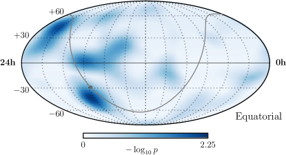
Figure 9: Two-year starting cascade skymap in equatorial coordinates (J2000). The skymap shows pre-trial $p$-values for all locations in the sky. The grey curve indicates the galactic plane, and the grey dot indicates the galactic center.

For the source candidate catalog search, an ensemble of 74 promising source candidates was selected a priori by merging previously studied catalogs of interesting galactic and extra-galactic objects (Aartsen et al., 2017a; Adrian-Martinez et al., 2016b). The result of the search is shown in Table 1. The most significant source is BL Lac, located at $(\alpha,\delta)=(330.68^{\circ},42.28^{\circ})$. The pre-trials significance is $p_{\text{pre}}=1.0\%$, and the best-fit number of signal events and spectral index are $\hat{n}_{s}=6.9$ and $\hat{\gamma}=3.0$, respectively. The post-trials significance is $p_{\text{post}}=36\%$. Flux upper limits for each object in the catalog are shown in Figure 10 along with the sensitivity and $5\sigma$ discovery potential as functions of declination.

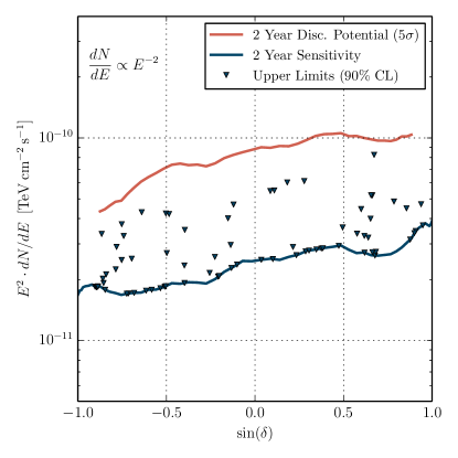
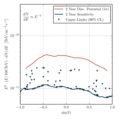
Figure 10: Sensitivity and $5\sigma$ discovery potential as functions of declination, with flux upper limits for each object in the source catalog. Left: hard spectral assumption ($\gamma=2$). Right: soft spectral assumption ($\gamma=3$).

Of the galactic plane searches, the southern-sky-only hypothesis test was more significant, with a pre-trials $p_{\text{pre}}=50\%$. The fit obtained $n_{s}=2.7$ and $\gamma=2$. This test is strongly correlated with the all-sky search; the post-trials significance is $p_{\text{post}}=65\%$.

6 Conclusion and Outlook

In this first search for sources of astrophysical neutrinos using cascades with energies as low as $1\,\mathrm{TeV}$ in two years of IceCube data, no significant source was found. This result is consistent with previous $\nu_{\mu}$ searches (Aartsen et al., 2017a; Adrian-Martinez et al., 2012; Adrian-Martinez et al., 2016b) which already find stringent constraints on emission from astrophysical point sources of neutrinos. Nevertheless, this analysis shows that despite large angular uncertainties, all-flavor source searches with cascades are surprisingly sensitive, particularly to emission from southern sources that follow a soft energy spectrum or are spatially extended. This type of analysis is therefore complementary to standard $\nu_{\mu}$ searches, which are most sensitive to point-like and northern sources.

Future source searches with cascades will benefit from several improvements. Most importantly, the adaptive veto method will soon be applied to at least four more years of IceCube data. Because of the low background in this event selection, the sensitivity strengthens faster than $[\text{detector livetime}]^{-1/2}$, as shown in Figure 11. Ongoing work on the optimization of cascade angular reconstructions, including increasingly detailed studies of Cherenkov light propagation in South Pole glacial ice, may lead to angular resolution improvements that increase the cascade channel signal-to-background ratio further still.

In this work, we searched for neutrino emission from a catalog of source candidates previously studied in track analyses (Aartsen et al., 2017a; Adrian-Martinez et al., 2016b). The catalog was optimized in light of the strengths of those analyses, and thus includes many northern sources which would almost certainly be visible first in throughgoing tracks. We may be able to improve the discovery potential for future catalog analyses with cascades by considering a catalog of source candidates for which this analysis is best-suited, such as extended objects in the southern sky.

We have considered only very simple models for extended emission from the galactic plane, which we have treated here as a uniform line source. However, detailed models (Ackermann et al., 2012; Gaggero et al., 2015) have been constructed to account for the measured distribution of $\gamma$ emission from poorly resolved sources and cosmic ray interactions with galactic dust clouds. Future cascade analyses will test these models directly, leading to clearer statements on neutrino emission within our own galaxy.

Here we have searched only for steady, time-independent neutrino emission, but the conclusions of this paper apply equally well to transient sources. While a cascade event selection has been added to IceCube’s gamma-ray burst analysis (Aartsen et al., 2016a), other time-dependent analyses (e.g. Aartsen et al., 2015e) have not yet made use of this channel. In the future, searches for emission from objects such as flaring AGN could benefit from the inclusion of neutrino-induced cascades. Proposed next-generation detectors (Aartsen et al., 2014b; Adrian-Martinez et al., 2016a) may also benefit by considering source searches with the cascade channel in the optimization of their optical sensors and array geometry.

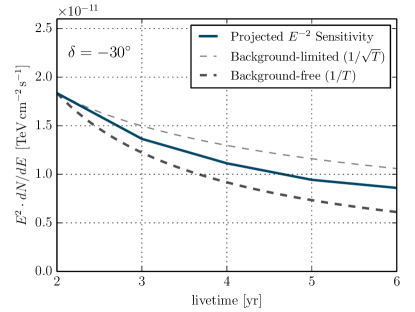
Figure 11: Projected sensitivity as a function of detector livetime for a source at $\delta=-30^{\circ}$. Time evolution scaling with $1/T$ (background-free case) and $1/\sqrt{T}$ (background-limited case) are shown in thick and thin grey dashed curves, respectively.

Table 1: Summary of the source catalog search. The objects are grouped by type, and within each type are sorted by increasing declination. The type, common name, and equatorial coordinates (J2000) are shown for each object. Where non-null ($\hat{n}_{s}>0$) results are found, the pre-trials significance $p_{\text{pre}}$ and best-fit $\hat{n}_{s}$ and $\hat{\gamma}$ are given.

Type	Source	$\alpha~{}(^{\circ})$	$\delta~{}(^{\circ})$	$p_{\text{pre}}$	$\hat{n}_{s}$	$\hat{\gamma}$
BL Lac	PKS 2005-489	302.37	$-48.82$	0.252	2.4	2.2
	PKS 0537-441	84.71	$-44.09$	0.256	1.7	1.8
	PKS 0426-380	67.17	$-37.93$	0.597	1.0	1.8
	PKS 0548-322	87.67	$-32.27$	0.634	1.2	2.2
	H 2356-309	359.78	$-30.63$	0.809	0.2	2.4
	PKS 2155-304	329.72	$-30.23$	0.642	1.2	2.4
	1ES 1101-232	165.91	$-23.49$	0.390	3.3	2.8
	1ES 0347-121	57.35	$-11.99$	0.543	2.5	3.8
	PKS 0235+164	39.66	$16.62$	$\cdot\cdot\cdot$	0.0	$\cdot\cdot\cdot$
	1ES 0229+200	38.20	$20.29$	$\cdot\cdot\cdot$	0.0	$\cdot\cdot\cdot$
	W Comae	185.38	$28.23$	0.618	0.6	3.8
	Mrk 421	166.11	$38.21$	$\cdot\cdot\cdot$	0.0	$\cdot\cdot\cdot$
	Mrk 501	253.47	$39.76$	0.404	1.5	2.6
	BL Lac	330.68	$42.28$	0.010	6.9	3.0
	H 1426+428	217.14	$42.67$	0.566	0.5	3.8
	3C66A	35.67	$43.04$	0.482	0.9	3.8
	1ES 2344+514	356.77	$51.70$	0.189	2.9	3.2
	1ES 1959+650	300.00	$65.15$	0.519	0.6	3.0
	S5 0716+71	110.47	$71.34$	$\cdot\cdot\cdot$	0.0	$\cdot\cdot\cdot$
Flat spectrum radio quasar	PKS 1454-354	224.36	$-35.65$	0.612	1.6	2.2
	PKS 1622-297	246.53	$-29.86$	0.286	3.6	2.2
	PKS 0454-234	74.27	$-23.43$	$\cdot\cdot\cdot$	0.0	$\cdot\cdot\cdot$
	QSO 1730-130	263.26	$-13.08$	0.365	4.5	3.8
	PKS 0727-11	112.58	$-11.70$	$\cdot\cdot\cdot$	0.0	$\cdot\cdot\cdot$
	PKS 1406-076	212.24	$-7.87$	0.375	5.6	3.8
	QSO 2022-077	306.42	$-7.64$	$\cdot\cdot\cdot$	0.0	$\cdot\cdot\cdot$
	HESS J1837-069	279.41	$-6.95$	0.121	8.9	3.8
	3C279	194.05	$-5.79$	0.754	0.9	3.8
	3C 273	187.28	$2.05$	0.718	0.9	2.8
	PKS 1502+106	226.10	$10.49$	0.057	9.1	3.8
	PKS 0528+134	82.73	$13.53$	$\cdot\cdot\cdot$	0.0	$\cdot\cdot\cdot$
	3C 454.3	343.49	$16.15$	0.066	7.4	3.8
	4C 38.41	248.81	$38.13$	0.391	1.6	2.4
Galactic center	Sgr A*	266.42	$-29.01$	0.080	5.6	2.2
Not identified	HESS J1507-622	226.72	$-62.34$	0.473	0.7	1.0
	HESS J1503-582	226.46	$-58.74$	0.438	0.7	1.0
	HESS J1741-302	265.25	$-30.20$	0.072	5.7	2.2
	HESS J1834-087	278.69	$-8.76$	0.180	7.5	3.8
	MGRO J1908+06	286.98	$6.27$	0.078	8.5	3.8
Pulsar wind nebula	HESS J1356-645	209.00	$-64.50$	0.795	0.1	3.8
	PSR B1259-63	197.55	$-63.52$	$\cdot\cdot\cdot$	0.0	$\cdot\cdot\cdot$
	HESS J1303-631	195.74	$-63.20$	$\cdot\cdot\cdot$	0.0	$\cdot\cdot\cdot$
	MSH 15-52	228.53	$-59.16$	0.408	0.7	1.0
	HESS J1023-575	155.83	$-57.76$	$\cdot\cdot\cdot$	0.0	$\cdot\cdot\cdot$
	HESS J1616-508	243.78	$-51.40$	0.166	2.4	2.0
	HESS J1632-478	248.04	$-47.82$	0.108	3.0	2.0
	Vela X	128.75	$-45.60$	$\cdot\cdot\cdot$	0.0	$\cdot\cdot\cdot$
	Geminga	98.48	$17.77$	$\cdot\cdot\cdot$	0.0	$\cdot\cdot\cdot$
	Crab Nebula	83.63	$22.01$	0.556	1.1	2.8
	MGRO J2019+37	305.22	$36.83$	0.224	3.5	3.6
Star formation region	Cyg OB2	308.08	$41.51$	0.135	4.2	3.4
Supernova remnant	RCW 86	220.68	$-62.48$	0.582	0.5	1.0
	RX J0852.0-4622	133.00	$-46.37$	$\cdot\cdot\cdot$	0.0	$\cdot\cdot\cdot$
	RX J1713.7-3946	258.25	$-39.75$	0.042	5.3	2.2
	W28	270.43	$-23.34$	0.159	4.3	2.2
	IC443	94.18	$22.53$	$\cdot\cdot\cdot$	0.0	$\cdot\cdot\cdot$
	Cas A	350.85	$58.81$	0.261	2.0	3.4
	TYCHO	6.36	$64.18$	$\cdot\cdot\cdot$	0.0	$\cdot\cdot\cdot$
Starburst/radio galaxy	Cen A	201.37	$-43.02$	0.629	1.0	2.6
	M87	187.71	$12.39$	0.438	1.8	2.6
	3C 123.0	69.27	$29.67$	0.379	2.2	3.0
	Cyg A	299.87	$40.73$	0.276	2.6	3.4
	NGC 1275	49.95	$41.51$	0.479	1.0	3.8
	M82	148.97	$69.68$	0.251	0.8	2.0
Seyfert galaxy	ESO 139-G12	264.41	$-59.94$	0.096	3.0	2.0
HMXB/mqso	Cir X-1	230.17	$-57.17$	0.372	0.8	1.0
	GX 339-4	255.70	$-48.79$	0.052	4.3	2.2
	LS 5039	276.56	$-14.83$	0.444	1.7	2.2
	SS433	287.96	$4.98$	0.086	8.7	3.8
	HESS J0632+057	98.25	$5.80$	$\cdot\cdot\cdot$	0.0	$\cdot\cdot\cdot$
	Cyg X-1	299.59	$35.20$	0.382	2.2	3.6
	Cyg X-3	308.11	$40.96$	0.137	4.2	3.4
	LSI 303	40.13	$61.23$	$\cdot\cdot\cdot$	0.0	$\cdot\cdot\cdot$
Massive star cluster	HESS J1614-518	63.58	$-51.82$	0.330	1.3	1.6

References

- Aartsen et al. (2013a) Aartsen, M. G., et al. 2013a, Science, 342, 1242856
- Aartsen et al. (2013b) —. 2013b, Nucl. Instrum. Meth., A711, 73
- Aartsen et al. (2014a) —. 2014a, JINST, 9, P03009
- Aartsen et al. (2014b) —. 2014b, arXiv:1412.5106
- Aartsen et al. (2014c) —. 2014c, Phys. Rev. Lett., 113, 101101
- Aartsen et al. (2014d) —. 2014d, Astrophys. J., 796, 109
- Aartsen et al. (2015a) —. 2015a, ICRC, 34, 1081
- Aartsen et al. (2015b) —. 2015b, Phys. Rev., D91, 022001
- Aartsen et al. (2015c) —. 2015c, Phys. Rev. Lett., 115, 081102
- Aartsen et al. (2015d) —. 2015d, Phys. Rev. Lett., 114, 171102
- Aartsen et al. (2015e) —. 2015e, Astrophys. J., 807, 46
- Aartsen et al. (2016a) —. 2016a, Astrophys. J., 824, 115
- Aartsen et al. (2016b) —. 2016b, Astrophys. J., 824, L28
- Aartsen et al. (2016c) —. 2016c, Astrophys. J., 833, 3
- Aartsen et al. (2017a) —. 2017a, Astrophys. J., 835, 151
- Aartsen et al. (2017b) —. 2017b, JINST, 12, P03012
- Abbasi et al. (2009) Abbasi, R., et al. 2009, Nucl. Instrum. Meth., A601, 294
- Abbasi et al. (2010) —. 2010, Nucl. Instrum. Meth., A618, 139
- Abbasi et al. (2012) —. 2012, Astropart. Phys., 35, 615
- Achterberg et al. (2006) Achterberg, A., et al. 2006, Astropart. Phys., 26, 155
- Ackermann et al. (2012) Ackermann, M., et al. 2012, Astrophys. J., 750, 3
- Adrian-Martinez et al. (2012) Adrian-Martinez, S., et al. 2012, Astrophys. J., 760, 53
- Adrian-Martinez et al. (2014) —. 2014, Astrophys. J., 786, L5
- Adrian-Martinez et al. (2015) —. 2015, ICRC, 34, 1078
- Adrian-Martinez et al. (2016a) —. 2016a, J. Phys., G43, 084001
- Adrian-Martinez et al. (2016b) —. 2016b, Astrophys. J., 823, 65
- Ahrens et al. (2004) Ahrens, J., et al. 2004, Nucl. Instrum. Meth., A524, 169
- Becker (2008) Becker, J. K. 2008, Phys. Rept., 458, 173
- Chirkin & Rhode (2004) Chirkin, D., & Rhode, W. 2004, arXiv:hep-ph/0407075
- Cooper-Sarkar et al. (2011) Cooper-Sarkar, A., Mertsch, P., & Sarkar, S. 2011, JHEP, 08, 042
- Gaggero et al. (2015) Gaggero, D., et al. 2015, Astrophys. J., 815, L25
- Gaisser et al. (1995) Gaisser, T. K., Halzen, F., & Stanev, T. 1995, Phys.Rept., 258, 173
- Glashow (1960) Glashow, S. L. 1960, Phys. Rev., 118, 316
- Learned & Mannheim (2000) Learned, J., & Mannheim, K. 2000, Ann. Rev. Nucl. Part. Sci., 50, 679
- Lehmann & Romano (2005) Lehmann, E. L., & Romano, J. P. 2005, Testing statistical hypotheses, 3rd edn., Springer Texts in Statistics (New York: Springer), xiv+784
- Neyman (1937) Neyman, J. 1937, Philos. Tr. R. Soc. A, 236, 333
- Radel & Wiebusch (2013) Radel, L., & Wiebusch, C. 2013, Astropart. Phys., 44, 102