Electronic and optical properties of graphite-related systems

Abstract

A systematic review is made for the AA-, AB- and ABC-stacked graphites. The generalized tight-binding model, accompanied with the effective-mass approximation and the Kubo formula, is developed to investigate electronic and optical properties in the presence/absence of a uniform magnetic field. The unusual electronic properties cover the stacking-dependent Dirac-cone structures, the significant energy widths along the stacking direction, the Landau subbands (LSs) crossing the Fermi level, the $B_{0}$-dependent LS energy spectra with crossings and anti-crossings, and the monolayer- or bilayer-like Landau wavefunctions. There exist the configuration-created special structures in density of states and optical spectra. Three kinds of graphites quite differ from one another in the available inter-LS excitation channels, including the number, frequency, intensity and structures of absorption peaks. The dimensional crossover presents the main similarities and differences between graphites and graphenes; furthermore, the quantum confinement enriches the magnetic quantization phenomena in carbon nanotubes and graphene nanoribbons. The cooperative/competitive relations among the interlayer atomic interactions, dimensions and magnetic quantization are responsible for the diversified essential properties. Part of theoretical predictions are consistent with the experimental measurements.

$\mathit{PACS}$: 73.20.At, 73.22.-f, 75.70.Ak

* Corresponding author.   Tel:  +886-6-275-7575;  Fax: +886-6-74-7995.
 E-mail address: mflin@mail.ncku.edu.tw (M.F. Lin)

Contents

1. Introduction ………………………………………………………………………………………………   01

2. Theoretical models ………………………………………………………………………………………   10

2.1 The magnetic tight-binding model for layered graphites ………………………………….   10

2.1.1 Simple hexagonal graphite graphene …………………………………………………………..   14

2.1.2 Bernal graphite ……………………………………………………………………………………….   16

2.1.3 Rhombohedral graphite …………………………………………………………………………..   17

2.1.4 The gradient approximation for optical properties ………………………………………..   20

3. Simple hexagonal graphite ……………………………………………………………………………   21

3.1 Electronic structures without external fields …………………………………………………   22

3.2 Optical properties without external fields ……………………………………………………   28

3.3 Magnetic quantization ……………………………………………………………………………..   31

3.3.1 Landau levels and wave functions ……………………………………………………………..   31

3.3.2 Landau subband energy spectra ………………………………………………………………   33

3.4 Magneto-optical properties ………………………………………………………………………….   39

4. Bernal graphite ………………………………………………………………………………………….   48

4.1 Electronic structures without external fields …………………………………………………..   48

4.2 Optical properties without external fields …………………………………………………….   54

4.3 Magnetic quantization ………………………………………………………………………………   56

4.3.1 Landau subbands and wave functions ……………………………………………………….   56

4.3.2 Anticrossings of Landau subbands …………………………………………………………….   60

4.4 Magneto-optical properties …………………………………………………………………………   63

5. Rhombohedral graphite ………………………………………………………………………………   71

5.1 Electronic structures without external fields …………………………………………………   71

5.2 Anisotropic Dirac cone along a nodal spiral ……………………………………………………   73

5.3 dimensional crossover ………………………………………………………………………………..   77

5.4 Optical properties without external fields ……………………………………………………..   79

5.5 Magneto-electronic properties …………………………………………………………………….   81

5.5.1 Tight-binding model ………………………………………………………………………………   81

5.5.2 Onsager quantization ………………………………………………………………………………   83

5.6 Magneto-optical properties ………………………………………………………………………   88

6. Quantum confinement in carbon nanotubes and graphene nanoribbons …………….   92

6.1 Magneto-electronic properties of carbon nanotubes ………………………………………..   93

6.2 Magneto-optical spectra of carbon nanotubes ……………………………………………….   99

6.3 Magneto-electronic properties of graphene nanoribbons ……………………………………   105

6.4 Magneto-optical spectra of graphene nanoribbons ……………………………………………   112

6.5 Comparisons and applications ……………………………………………………………………..   120

7. Concluding remarks …………………………………………………………………………………….   126

Acknowledgments …………………………………………………………………………………………..   135

References (Ref. 1-Ref. 233) …………………………………………………………………………….   135

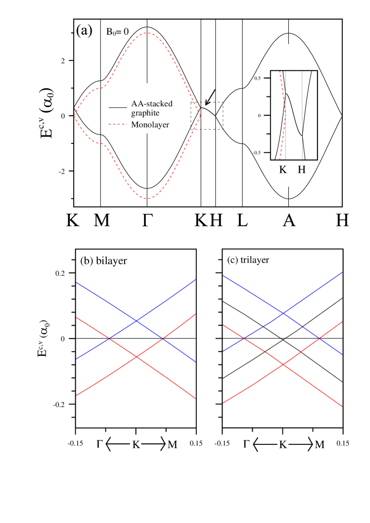
Figure 1: Band structures for AA-stacked (a) graphite and monolayer graphene; (b) bilayer and (c) trilayer systems.

Figure captions (Fig. 1-Fig. 49) ……………………………………………………………………….   171

1 Introduction

Carbon atoms can form various condensed-matter systems with unique geometric structures, mainly owing to four active atomic orbitals. From three- to zero-dimensional carbon-related systems cover diamond,[1] graphite,[3, 2, 4] graphene,[5] graphene nanoribbons,[6] carbon nanotube,[7] and carbon fullerene.[8] Most of them have the ${sp^{2}}$ bonding except for the ${sp^{3}}$ bonding in diamond. The former might exhibit similar physical properties, e.g., the $\pi$-electronic optical excitations.[9, 10] Graphite is one of the most extensively studied materials theoretically and experimentally. This layered system is very suitable for exploring the diverse 3D and 2D phenomena. The interplane attractive forces originate from the weak Van der Waals interactions of the ${2p_{z}}$ orbitals. The honeycomb lattice and the stacking configuration are responsible for the unique properties of graphite, e.g., the semi-metallic behavior due to the hexagonal symmetry and the interlayer atomic interactions. The essential properties are dramatically changed by the intercalation of various atoms and molecules. Graphite intercalation compounds could achieve a conductivity as good as copper.[11, 12, 4, 13] In general, there exist three kinds of ordered configurations in the layered graphites and compounds, namely AA, AB and ABC stackings. Simple hexagonal, Bernal and rhombohedral graphites exhibit the rich and diverse electronic and optical properties in the presence/absence of a uniform magnetic field (${\bf B}$=${B_{0}\hat{z}}$). To present a systematic review of them, the generalized tight-binding model is developed under the magnetic quantization. This model, combined with the Kubo formula, is utilized to investigate the essential properties of layered carbon-related systems. The dimensional crossover from graphene to graphite and the quantum confinement in nanotube and nanoribbon systems are discussed thoroughly. A detailed comparison with the other theoretical studies and the experimental measurements is also made.

Few- and multi-layer graphenes, with distinct stacking configurations, are successfully produced by various experimental methods since the first discovery of monolayer graphene in 2004 by the mechanical exfoliation.[5] They possess the hexagonal symmetry and the nanoscale size, leading to a lot of remarkable characteristics, e.g., the largest Young s modulus,[15] feature-rich energy bands,[16, 17] diverse optical selective rules,[25, 19, 18, 20, 21, 22, 23, 24] unique magnetic quantization,[35, 224, 27, 28, 29, 30, 31, 32, 33, 34] anomalous quantum Hall effects,[36, 37, 38, 39, 40] and multi-mode plasmons.[41, 42, 43, 44] Their electronic and optical properties are very sensitive to the changes in the stacking configuration,[33, 34, 31, 29, 224, 16] layer number,[31, 29, 16, 224] magnetic field,[32, 31, 30, 28, 29, 18, 19, 20, 21, 22, 23, 24, 224, 27, 17] electric field,[32, 17] mechanical strain,[16, 17] doping,[16, 17] and sliding.[35] Five kinds of electronic structures, linear,[224] parabolic,[31, 224, 27] partially flat,[31, 224] sombrero-shaped,[32, 31, 224] and oscillatory[32, 34, 35] energy bands, are revealed in AB and ABC stacking systems. The last ones could be created by a perpendicular electric field. However, the AA stacking only has the first kind. Specifically, the intersection of the linear valence and conduction bands can form the so-called Dirac-cone structure. The main features of energy bands are directly reflected in the other essential properties. The finite-layer confinement effects are expected to induce important differences between the layered graphenes and graphites. The close relations arising from the dimensional crossover deserve a thorough investigation.

Graphite crystals are made up of a series of stacked graphene plane. Among three kinds of ordered stacking configurations, the AB-stacked graphite is predicted to have the lowest ground state energy according to the first-principles calculations.[45] Nature graphite presents the dominating AB stacking and the partial ABC stacking.[2, 3] The AA-stacked graphite, which possesses the simplest crystal structure, does not exist naturally. The periodical AA stacking is first observed in the Li-intercalation graphite compounds[4] with high free electron density and super conducting transition temperature at  1.9 K.[14] Simple hexagonal graphite is successfully synthesized by using the dc plasma in hydrogen-methane mixtures,[46] and AA-stacked graphenes are generated by the method of Hummers and Offeman and the chemical-vapor deposition (CVD). [47, 48] Furthermore, the AA stacking sequence is confirmed from the high-resolution transmission electron microscopy (HRTEM).[47] Specifically, angle-resolved photoemission spectroscopy (ARPES), a powerful tool in the direct identification of energy bands, is utilized to examine two/three pairs of Dirac-cone structures in bilayer/trilayer AA stacking.[49, 50]

The AA stacking systems have stirred a lot of theoretical researches, such as band structures,[52, 51, 31, 52, 29] magnetic quantization,[53, 54, 31, 224, 29] optical properties,[55, 56, 57] Coulomb excitations,[58, 341, 60, 61, 62] quantum transport,[63] and phonon spectra,[64] Simple hexagonal graphite, a 3D layered system with the same graphitic sheets on the $(x,y)$-plane, is first proposed by Charlier et al.[45] From the tight-binding model and the first-principles method, this system belongs to a band-overlap semimetal, in which the same electron and hole density originate from the significant interlayer atomic interactions. There is one pair of low-lying valence and conduction bands. The critical feature is the vertical Dirac-cone structure with the sufficiently wide bandwidth of $\sim 1$ eV along the ${k_{z}}$-direction (${\bf k}$ wave vector). Similarly, the AA-stacked graphenes is predicted to exhibit multiple Dirac cones vertical to one another.[224, 29, 51] Moreover, Bloch wave functions are only the symmetric or anti-symmetric superposition of the tight-binding functions on the distinct sublatticesa and layers.[224] Apparently, these 3D and 2D vertical Dirac cones will dominate the other low-energy essential properties, e.g., the special structures in density of states (DOS),[224, 52, 53] the quantized Landau subbands (LSs) and levels (LLs),[224, 29, 54] the rich optical spectra,[56, 57] and the diversified plasmon modes.[58, 341, 60, 61, 62] The magnetic quantization is frequently explored by the effective-mass approximation[29] and the generalized tight-binding model.[224, 31] It is initiated from the vertical Dirac points, the extreme points in the energy-wave-vector space. This creates the specific $B_{0}$-dependent energy spectra and the well-behaved charge distributions, thus leading to the diverse and unique magneto-absorption peaks, e.g., the intraband and interband inter-LS excitations, the multi-channel threshold peaks, and beating-form absorption peaks in AA-stacked graphite.[54, 56, 57] The predicted band structures, energy spectra and optical excitations could be verified by ARPES,[49, 50] scanning tunneling spectroscopy (STS)^Refs and optical spectroscopy, [20, 21, 22, 23, 24] respectively.

Bernal graphite is a well-known semimetal,[2] with conduction electron concentration of $\sim{5\times\,10^{18}}/cm^{3}$. Furthermore, the AB stacking configuration is frequently observed in the layered systems, e.g., bilayer,[5, 65] trilayer,[66, 65, 67] and tetralayer graphenes.[65] The AB-stacked graphite possesses two pairs of low-lying energy bands dominated by the ${2p_{z}}$ orbitals, owing to a primitive unit cell with two neighboring layers. The highly anisotropic band structure, the strong and weak energy dispersions along the ${(k_{x},k_{y})}$ plane and $k_{z}$-axis, respectively, is confirmed by the ARPES measurements.[178, 179, 180, 181, NatPhy2;595PRL100;037601] The similar examinations are done for two pairs of parabolic bands in bilayer AB stacking,[176, 177] and the linear and parabolic bands in trilayer system[176, 69]. The measured DOS of Bernal graphite presents the splitting $\pi$ and $\pi^{\ast}$ peaks at the middle energy,[188] reflecting the highly accumulated states near the saddle points. Furthermore, it is finite near the Fermi level ($E_{F}$) because of the semi-metallic behavior.[189] An electric-field-induced band gap is observed in bilayer AB stacking.[66] The magnetically quantized energy spectra, with many special structures, are also identified using the STS measurements for the AB-stacked graphite[74, 75] and graphenes,[76, 77] especially for the square-root and linear dependences on the magnetic-field strength (the monolayer- and bilayer-like behaviors at low energy). From the optical measurements, Bernal graphite shows a very prominent $\pi$-electronic absorption peak at frequency $\sim 5$ eV,[78] as revealed in carbon-related systems with the ${sp^{2}}$ bonding.[79, 80] Concerning the low-frequency magneto-optical experiments, the measured excitation spectra due to LSs[87, 88, 81, 82, 83, 84, 85] or LLs[19, 18, 20, 21, 22, 23, 24] clearly reveal a lot of pronounced absorption structures, the selection rule of ${\triangle\,n=\pm\,1}$ ($n$ quantum number), and the strong dependence on the wave vector of $k_{z}$ or the layer number ($N$).

The earliest attempt to calculate the band structures of monolayer graphene and Bernal graphite is done by Wallace using the tight-binding model with the atomic interactions of ${2p_{z}}$ orbitals.[89] The former 2D system has the linear valence and conduction bands intersecting at $E_{F}$, so that it belongs to a zero-gap semiconductor with vanishing DOS there. However, the semi-metallic 3D electronic structure is further comprehended from the Slonczewski-Weis-McClure Hamiltonian involving the important intralayer and interlayer atomic interactions.[90, 91] The magnetic Hamiltonian could be solved by the low-energy perturbation approximation, in which the LS energy spectra exhibit the crossing and anti-crossing behaviors.[93, 94] The generalized tight-binding model, which deals with the magnetic field and all atomic interactions simultaneously, is developed to explore the main features of LSs, e.g., two groups of valence and conduction LSs, and the layer-, $k_{z}$- and $B_{0}$-dependent spatial oscillation modes.[92, 81] As to the AB-stacked graphenes, their electronic and magneto-electronic properties present the bilayer- and monolayer-like behaviors, being associated with two pair of parabolic bands and a slightly distorted Dirac cone, respectively.[16, 224] The former is only revealed in the odd-$N$ systems. Optical spectra of AB-stacked systems are predicted to exhibit the strong dependence of special structures on the layer number and dimension.[18, 19, 20, 21, 22, 23, 24, 82] The magneto-optical excitations arising from two groups of LSs in graphite or $N$ groups of LLs in graphenes could be evaluated from the generalized tight-binding model.[81] On the other hand, those due to the first group of LLs/LLs is frequently investigated by the effective-mass approximation in detail.[93, 94] The calculated electronic and optical properties are in agreement with the experimental measurements.[74, 75]

Rhombohedral phase is usually found to be mixed with Bernal phase in natural graphite. The ABC stacking sequence in bulk graphite is directly identified from the experimental measurements of HRTEM,[95] X-ray diffraction,[96, 97, 98] and scanning tunneling microscopy (STM).[99, 100] Specifically, this stacking configuration could account for the measured 3D quantum Hall effect with multiple plateau structures,[122] since rhombohedral graphite possesses the well separated LS energy spectra.[124, 232] In addition, doped Bernal graphite is predicted to exhibit only one plateau.[101] Both ABC- and AB-stacked graphenes can be produced by mechanical exfoliation of kish graphite,[102, 103] CVD,[104, 105, 106, 107] chemical and electrochemical reduction of graphite oxide,[108, 109, 110] arc discharge,[111, 112, 113] flame synthesis,[114] and electrostatic manipulation of STM.[115, 187] The ARPES measurements have verified the partially flat, sombrero-shaped and linear bands in tri-layer ABC stacking.[69] As to the STS spectra, a pronounced peak at the Fermi level characteristic of the partial flat band is revealed in tri-layer and penta-layer ABC stacking.[187, 118, 117] Moreover, infrared reflection spectroscopy and absorption spectroscopy are utilized to examine the low-frequency optical properties, displaying a clear evidence of two featured absorption structures due to the partially flat and sombrero-shaped energy bands.[230] According to the specific infrared conductivities, infrared scattering scanning near-field optical microscopy can distinguish the ABC stacking domains with nano-scaled resolution from other domains. However, the magneto-optical measurements on ABC-stacked graphenes are absent up to now.

The ABC-stacked graphite has a rhombohedral unit cell, while the AA- and AB-stacked systems possess the hexagonal ones. This critical difference in stacking symmetry is responsible for the diversified essential properties. Among three kinds of bulk graphites, rhombohedral graphite is expected to present the smallest band overlap (the lowest free carrier density), and the weakest energy dispersion along the $k_{z}$-direction.[119, 221, 121] There also exists a robust low-energy electronic structure, a 3D spiral Dirac-cone structure. This results in the unusual magnetic quantization,[124, 232, 125] in which the quantized LSs exhibit the monolayer-like behavior and the significant $k_{z}$-dependence. The previous studies show that four kinds of energy dispersions exist in the ABC-stacked graphenes.[224, 31] Specially, the partially flat bands corresponding to the surface states and the sombrero-shaped bands are absent in bulk system. They can create the diverse and unique LLs, with the asymmetric energy spectra about $E_{F}$, the normal and abnormal $B_{0}$-dependences, the well-behaved and distorted probability distributions, and the frequent crossings and anti-crossings.[224, 31] Apparently, optical and magneto-optical properties are greatly enriched by the layer number and dimension.[128, 129, 126, 220] The quantized LLs of the partially flat bands and the lowest sombrero-shaped band have been verified by the magneto-Raman spectroscopy for a large ABC domain in a graphene multilayer flake.[218] Layered graphenes are predicted to have more complicated excitation spectra, compared with 3D system. The former and the latter, respectively, reveal N² categories of inter-LL transitions and one category of inter-LS excitations.[128, 220]

In addition to the stacking configurations, the distinct dimensions can create the diverse phenomena in carbon-related systems. The quantum confinement in 1D carbon nanotubes and graphene nanoribbons play a critical role in the essential properties. The systematic studies have been made for the former since the successful synthesis using the arc-discharge evaporation in 1991.[7] Each carbon nanotube could be regarded as a rolled-up graphene sheet in the cylindrical form. It is identified to be a metal or semiconductor, depending on the radius and chiral angle.[130, 131, 132] The geometry-dependent energy spectra, with energy gaps ($E_{g}$’s), are directly verified from the STS measurements.[193, 194] Specifically, the cylindrical symmetry can present the well-known Aharonov-Bohm effect under an axial magnetic field.[142, 143, 144, 141] This is confirmed by the experimental measurements on optical[145, 146] and transport properties.[149, 147, 148] However, a closed surface acts as a high barrier in the formation of the dispersionless LLs, since a perpendicular magnetic field leads to a vanishing flux through carbon hexagons. It is very difficult to observe the physical phenomena associated with the highly degenerate states except for very high field strength.[150]

The essential properties are greatly enriched by the boundary conditions in 1D systems. The open and periodical boundaries, which, respectively, correspond to graphene nanoribbon and carbon nanotube, induce the important differences between them. A graphene nanoribbon is a finite-width graphene or an unzipped carbon nanotube. Graphene nanoribbons could be produced by cutting few-layer graphenes,[151, 152] unzipping multi-walled carbon nanotubes,[155, 153, 154] and using the direct chemical syntheses.[156, 157, 158] The cooperative or competitive relations among the open boundary, the edge structure, and the magnetic field are responsible for the rich and unique properties. The 1D parabolic bands, with energy gaps, in armchair graphene nanoribbons, are confirmed by ARPES.[133] Furthermore, STS has verified the asymmetric DOS peaks and the finite-size effect on energy gap.[134, 135, 136, 137] Optical spectra are predicted to have the edge-dependent selection rules.[139, 138, 140] The theoretical calculations show that only the quasi-LLs (QLLs), with partially dispersionless relations, could survive in the presence of a perpendicular magnetic field.[159, 160] The magneto-optical selection rule, as revealed in layered graphenes, sharply contrasts with that in carbon nanotubes with the well-defined angular momenta along the azimuthal direction.[161]

In this work, we propose and develop the generalized tight-bindings model to fully comprehend the electronic and optical properties of the graphite-related systems. The Hamiltonin is built from the tight-binding functions on the distinct sublattices and layers, in which all important atomic interactions, stacking configuration, layer number and external fields are taken into account simultaneously. A quite large Hamiltonian matrix, being associated with the periodical variation of the vector potential, is solved by an exact diagonalization method. The essential properties can be evaluated very efficiently. Moreover, the effective-mass approximation is utilized to provide the qualitative behaviors and the semi-quantitative results, e.g., the layer-dependent characteristics. Specifically, the Onsager quantization method is also introduced to understand the magnetic LS energy spectra in the ABC-stacked graphite with the unique spiral Dirac cones. Such approximations are useful in the identification of the critical atomic interactions creating the unusual properties.

The AA-, AB- and ABC-stacked graphites and graphenes, and 1D graphene nanoribbons and carbon nnaotubes are worthy of a systematic review of essential properties. Electronic and optical properties, which mainly come from carbon ${2p_{z}}$ orbitals, are investigated in the presence/absence of magnetic field. Electronic structures, quantized LS and LL state energies, magnetic wave functions, DOS and optical spectral functions are included in the calculated results. Band widths, energy dispersion relations, critical points in energy-wave-vector space, crossings and anti-crossings of $B_{0}$-dependent energy spectra, spatial oscillation modes of localized probability distributions, and various special structures in DOS are explored in detail. The main features of optical excitations focus on tht available excitation channels, the form, number, intensity and frequency of prominent absorption structures, and the layer/dimension and field dependences. Moreover, the theoretical predictions are compared with the ARPES, STS and optical measurements and require more experimental examinations. Chapter 2 covers geometric structures, important atomic interactions, the generalized tight-binding model, and the Kubo formula, in which the main issues are the construction of the magnetic Hamiltonians and the efficient combination two methods. In chapter 3, the stacking- and layer-enriched essential properties are studied for the AA-stacked graphite and graphenes, especially for those due to the vertical multiple Dirac-cone structures. The analytical band structures and magneto-electronic energy spectra are obtained from the approximate expansions about the high symmetry points. They are available in illustrating the diversified characteristics, e.g., the determination of the close relations between the absorption spectra and the important intralayer/interlayer atomic interactions. The dimensional crossover from monolayer graphene to graphite creates the critical differences of 2D and 3D phenomena, including the semiconductor-semimetal transition, the $k_{z}$-dependent band width, the LS/LL energy spectra near the Fermi level, the optical gap, and the low- and middle-frequency absorption structures.

The dramatic transformations of essential properties are clearly revealed in distinct stacking configurations. As to the AB-stacked systems, the linear and parabolic energy dispersions, the crossings and anti-crossings of LS/LL energy spectra, the well-behaved and perturbed magnetic wave functions, the layer- and dimension-dependent optical spectra; the rich magneto-absorption peaks are investigated in Chap. 4. The monolayer- and bilayer-like behaviors are presented for Bernal graphite and layered AB stacking. Specifically, ABC-stacked graphenes has the linear, parabolic, partially flat and Sombrero-shaped energy bands, while rhombohedral graphite exhibits a 3D spiral Dirac-cone structure, as indicated in Chap. 5. Such characteristics are expected to create the unique essential properties. The low-energy approximation and magnetic quantization are proposed to explain the diversified electronic properties and optical spectra. In chapter 6, the reduced dimension in graphene nanoribbons and carbon nanotubes leads to the rich essential properties being sensitive to the open/periodical boundary condition, width/radius, edge/chiral angle, and external fields. Comparisons among the graphite-related systems and potential applications are also discussed. Finally, chapter 6 contains concluding remarks and outlook. The theoretical framework could be further extended to the other main-stream layered materials.

2 Theoretical models

In the presence of a uniform magnetic field, $\mathbf{B}=B_{0}\hat{z}$, electrons are forced to undergo the cyclotron motion in the x-y plane. As a result, electronic states are evolved into highly degenerate states, called Landau subbands (LSs) in graphites. The 1D LSs are calculated from the subenvelope functions established on different sublattices in the framework of the generalized tight-binding model, which simultaneously takes into account external fields and atomic interactions. The magneto Hamiltonian is built from the tight-binding functions coupled with a periodic Peierls phase in an enlarged unit cell; the period depends on the commensurate relation between the lattice constant and the Peierls phase. According to the Kubo formula, it could further be utilized to comprehend the main features of magneto-absorption spectra, which are closely related to the Landau-level spectrum and the transition matrix elements. The method provides accurate and reliable results for a wide-energy range. The three prototypical configurations of bulk graphites, namely, simple hexagonal, Bernal and rhombohedral graphites, are chosen for a systematic review. The magnetic quantization in 3D graphene systems shows interesting phenomena as a function the stacking configuration and the magnetic field strength.

2.1 The magnetic tight-binding model for layered graphites

The geometric structures of simple hexagonal, Bernal and rhombohedral bulk graphites are shown in Figs. 1(a)-1(c). They are, respectively, constructed from 2D graphene layers periodically stacked along $\widehat{z}$ with AA, AB and ABC stacking configurations, where the layer-layer distance $I_{z}$ is set as $3.35$ ${\AA}$. Detailed definitions of the stacking sequences are made in following sections. The unit cells of different graphites are marked by the gray shadows, which contain two sublattices, $A^{l}$ and $B^{l}$, on each layer, where $l$ represents the number of the layer, and the symbols $\alpha$’s, $\beta$’s and $\gamma$’s indicate the intrelayer and intralayer hopping integrals. The first Brillouin zone is a hexagonal prism, as shown in Fig. 1(e), where the highly symmetric points are defined as $\Gamma$, M, K, A, L and H. The KH lengths for the AA, AB, and ABC stackings are, respectively, equal to $\pi/I_{z}$, $\pi/2I_{z}$, and $\pi/3I_{z}$ based on the periods along $\widehat{z}$.

In general, the essential physical properties are mainly determined by 2$p_{z}$ orbitals of carbon atoms. Built from the subspace spanned by the tight-binding functions $\varphi_{A^{l}}$ and $\varphi_{B^{l}}$($l=1,2....$), the wave function is characterized by their linear combination over all $A$ and $B$ sublattices in a unit cell:

$$\Psi=\sum_{l}C_{A^{l}}\varphi_{A^{l}}+C_{B^{l}}\varphi_{B^{l}},$$ (1)

where $C_{A^{l}}$ and $C_{B^{l}}$ are normalization factors. The tight-binding functions are

$$\begin{array}[]{l}\varphi_{A^{l}}=\sum_{{R}_{A^{l}}}\exp(i\mathbf{k}\cdot\mathbf{R}_{A^{l}})\chi(\mathbf{r}-\mathbf{R}_{A^{l}})\\ \varphi_{B^{l}}=\sum_{{R}_{B^{l}}}\exp(i\mathbf{k}\cdot\mathbf{R}_{B^{l}})\chi(\mathbf{r}-\mathbf{R}_{B^{l}}),\end{array}$$ (4)

where $\chi(\mathbf{r})$ is the atomic 2$p_{z}$ orbital of an isolated carbon, and $\mathbf{R}$ is the position vector of an atom.

The effective momentum in the presence of ${\bf B}$ is $\mathbf{P}-e\mathbf{A}/c$, so that the 3D electronic bands of bulk graphites are quantized into the so-called 1D LSs. A periodic Peierls phase $G_{R}\equiv{\frac{2{\pi}}{{\phi}_{0}}}$ $\int_{\mathbf{R}^{\prime}}^{\mathbf{R}}\mathbf{A}(\mathbf{r})\cdot d\mathbf{r}$ is introduced to the tight-binding functions in Eqs. (2) and (3), where $\mathbf{A}$ is the vector potential and $\phi_{0}=2\pi\hbar c/e$ ($4.1356\times 10^{-15}$ [T$\cdot$m${}^{2}]$) is the flux quantum. The Hamiltonian element coupled with the Peierls phase factor is given by

$$H^{B}_{i,j}=H_{i,j}e^{i\Delta G_{i,j}}=H_{i,j}e^{i{\frac{2{\pi}}{{\phi}_{0}}}\int_{\mathbf{R_{j}}}^{\mathbf{R_{i}}}\mathbf{A}(\mathbf{r})\cdot d\mathbf{r}}\text{.}$$ (5)

The phase factor gives rise to an enlargement of the primitive unit cell (Fig. 1(d)), depending on the commensurate period of the lattice and the Peierls phase. Using the Landau gauge $\mathbf{A}=(0,B_{0}x,0)$, the period of the phase is $l=3R_{B}b\hat{x}$, in which there are $2R_{B}$ $A$ and $2R_{B}$ $B$ atoms in an enlarged unit cell ($R_{B}=\frac{\phi_{0}/(3\sqrt{3}b^{\prime 2}/2)}{B_{0}}\simeq\frac{79000\text{ T}}{B_{0}}$). This implies that the wave functions of graphites under a uniform magnetic field can be characterized by the subenvelope functions spanned over all bases in the enlarged unit cell, the zero points of which are used to define the quantum numbers of LSs. The wavefunction is decomposed into two components in the magnetically enlarged unit cell as follows:

$$|\Psi_{\mathbf{k}}\rangle=\sum\limits_{m=1}^{2R_{B}-1}(A_{o}|A_{m\mathbf{k}}\rangle+B_{o}|B_{m\mathbf{k}}\rangle)+\sum\limits_{m=1}^{2R_{B}}(A_{e}|A_{m\mathbf{k}}\rangle+B_{e}|B_{m\mathbf{k}}\rangle)\text{,}$$ (6)

where $o$ and $e$, respectively, represent the odd-indexed and even-indexed parts. The subenvelope function $A_{o,e}$ ($B_{o,e}$), described by an $n$-th order Hermite polynomial multiplied with a Gaussian function, is even or odd spatially symmetric and represents the probability amplitude of wavefunction contributed by each carbon atom. Considering the Peierls substitution for interlayer and intralayer atomic interactions, we can obtain the explicit form of the magnetic Hamiltonian matrix of bulk graphites. A procedure for the band-like Hamiltonian matrix is further introduced to efficiently solve the eigenvectors and eigenvalues by choosing an appropriate sequence for the bases. In the following sections, the Hamiltonian matrices are derived for the simple hexagonal, Bernal and rhombohedral graphites in the generalized tight-binding model.

2.1.1 Simple hexagonal graphite

Simple hexagonal graphite, as shown in Fig. 1(a), has each layer periodic along $\hat{z}$ with the same x-y projection. The primitive unit cell includes only two atoms same as that of monolayer graphene. Four important atomic interactions are used to describe the electronic properties, i.e., $\alpha_{0}(=2.569$ eV), $\alpha_{1}(=0.361$ eV), $\alpha_{2}(=0.013)$ eV and $\alpha_{3}(=-0.032$ eV),[52] respectively coming from the intralayer hopping between nearest-neighbor atoms, the interlayer vertical hoppings between nearest- and next-nearest-neighbor planes, and non-vertical hopping between nearest-neighbor planes.

The zero-field Hamiltonian matrix in the subspace of tight-binding basis $\{\varphi_{A},\varphi_{B}\}$ is expressed as

$$H_{AA}=\left\{\begin{array}[]{cc}\alpha_{1}h+\alpha_{2}(h^{2}-2)&f(k_{x},k_{y})(\alpha_{0}+\alpha_{3}h)\\ f^{*}(k_{x},k_{y})(\alpha_{0}+\alpha_{3}h)&\alpha_{1}h+\alpha_{2}(h^{2}-2)\\ \end{array}\right\}\text{,}$$ (7)

where $f(k_{x},k_{y})=\sum_{j=1}^{3}\exp(i\mathbf{k}\cdot\mathbf{r}_{j})=\exp(ibk_{x})+\exp(ibk_{x}/2)\cos(\sqrt{3}bk_{y}/2)$ represents the phase summation arising from the three nearest neighbors, and $h=2\cos(k_{z}I_{z})$. The $k_{z}$-dependent terms are involved in the matrix elements due to the periodicity along the $z$-direction. The $\pi$-electronic energy dispersions are obtained from diagonalizing the Hamiltonian matrix in Eq. (5):

$$E^{c,v}_{\pm}(k_{x},k_{y},k_{z})=\alpha_{1}h+2\alpha_{2}[h^{2}/2-1]\pm(\alpha_{0}+\alpha_{3}h)|f(k_{x},k_{y})|,$$ (8)

and wave functions are

$$\Psi^{c,v}_{\pm,\mathbf{k}}=\frac{1}{\sqrt{2}}\{\Psi_{\mathbf{k}}^{A}\pm\frac{f^{*}(k_{x},k_{y})}{|f(k_{x},k_{y})|}\Psi_{\mathbf{k}}^{B}\}.$$ (9)

The superscripts $c$ and $v$, respectively, represent the conduction and valence states.

As a result of the vector-potential-induced phase, the number of bases in the primitive unit cell is increased by $2R_{B}$ times compared to the zero-field case. Using the Peierls substitution of Eq. (4) and considering only the neighboring atoms coupled by $\alpha$’s, one can derive a band-like form for the magnetic Hamiltonian matrix of the AA-stacked graphite

$$\langle B_{mk}|H|B_{m^{\prime}k}\rangle = \langle A_{mk}|H|A_{m^{\prime}k}\rangle{=[\alpha_{1}h+\alpha_{2}(h^{2}-2)]{\delta_{m,m^{\prime}}}}\text{,}$$ (10)

$${{\langle A_{mk}|H|B_{m^{\prime}k}\rangle}} {=} {{(\alpha_{0}+\alpha_{3}h)}}[t_{1k}(m)\delta_{m,m^{\prime}}+q\delta_{m-1,m^{\prime}}]\text{,}$$ (11)

where the eigenvector is expanded in the bases with the specific sequence
$\{{A_{1k},B_{2R_{B}k},B_{1k},A_{2R_{B}k},........B_{R_{B}k},A_{R_{B}+1k}}\}$. The independent phase terms are

$$\begin{gathered}\\ t_{1k}(m)=exp\{i[-(k_{x}b/2)-(\sqrt{3}k_{y}b/2)+\pi\Phi(i-1+1/6)]\},\hfill\\ \\ t_{2k}(m)=exp\{i[-(k_{x}b/2)-(\sqrt{3}k_{y}b/2)+\pi\Phi(i-1+3/6)]\},\hfill\\ \\ q=exp\{ik_{x}b\}.\hfill\\ .\end{gathered}$$ (12)

By diagonalizing the matrix in Eqs. (8) and (9), the $k_{z}$-dependent energies and wave functions of the valence and conduction LSs are thus obtained. Such a band-like matrix spanned by a specific order of the bases is also applicable to other prototypes bulk graphites. In addition, when the low-energy approximation, related to the Dirac points, is made for the Hamiltonian matrix in Eq. (5), the LSs spectra are further evaluated from the magnetic quantization (discussion in 3.3.2).^Ref However, the conservation of 3D carrier density needs to be included in this evaluation.

2.1.2 Bernal graphite

Bernal graphite is the primary component of the natural graphites. The primitive unit cell comprises $A^{1}$, $B^{1}$, $A^{2}$ and $B^{2}$ atoms on two adjacent layers, where $A^{1}$ and $A^{2}$ ($B^{1}$ and $B^{2}$) are directly located above or below $A^{2}$ and $A^{1}$ (the centers of hexagons) in adjacent layers, a configuration namely AB stacking (Fig. 1(b)). The critical atomic interactions based on Slonczewski-Weiss-McClure (SWM) model cover $\gamma_{0},.....,\gamma_{5}$, which are interpreted as hopping integrals between nearest-neighbor and next-nearest-neighbor atoms, and additionally $\gamma_{6}$, which refers to the difference of the chemical environments between non-equivalent $A$ and $B$ atoms. The values are as follows: $\gamma_{0}=3.12$ eV, $\gamma_{1}=0.38$ eV, $\gamma_{2}=-0.021$ eV, $\gamma_{3}=0.28$ eV, $\gamma_{4}=0.12$ eV, $\gamma_{5}=-0.003$ eV and $\gamma_{6}=-0.0366$ eV.[45]

The tight-binding Hamiltonian is described by a $4\times 4$ matrix, which, expanded in the basis $\{{\varphi_{A^{1}},\varphi_{B^{1}},\varphi_{B^{2}},\varphi_{A^{2}}}\}$, takes the form

$$H_{AB}=\left\{\begin{array}[]{cccc}E_{A}&\gamma_{0}f(k_{x},k_{y})&\gamma_{1}h&\gamma_{4}hf^{*}(k_{x},k_{y})\\ \gamma_{0}f^{*}(k_{x},k_{y})&E_{B}&\gamma_{4}hf^{*}(k_{x},k_{y})&\gamma_{3}hf(k_{x},k_{y})\\ \gamma_{1}h&\gamma_{4}hf(k_{x},k_{y})&E_{A}&\gamma_{0}f^{*}(k_{x},k_{y})\\ \gamma_{4}hf(k_{x},k_{y})&\gamma_{3}hf^{*}(k_{x},k_{y})&\gamma_{0}f(k_{x},k_{y})&E_{B}\\ \end{array}\right\}\text{,}$$ (13)

where $E_{A}=\gamma_{6}+\gamma_{5}h^{2}/2$ and $E_{B}=\gamma_{2}h^{2}/2$ indicate the sum of the on-site energy and the hopping energy of A and B atoms, respectively. Energy bands and wave functions are easily calculated from diagonalizing the Hamiltonian matrix.

At $\mathbf{B}=B_{0}\widehat{z}$, the magnetically enlarged unit cell includes $2\times 4R_{B}$ bases, which constructs the $k_{z}$-dependent Hamiltonian matrix with non-zero terms only between neighboring sublattices on same and different layers. An explicit form of the matrix elements is given by

$$\langle B_{mk}^{1}|H|A_{mk^{\prime}}^{1}\rangle = -\gamma_{0}(t_{1}(m)\delta_{m,m^{\prime}}+q\delta_{m+1,m^{\prime}}),$$ (14)

$$\langle B_{mk}^{1}|H|A_{mk^{\prime}}^{2}\rangle = \gamma_{4}h(t_{1}(m)\delta_{m,m^{\prime}}+q\delta_{m+1,m^{\prime}}),$$ (15)

$$\langle A_{mk}^{2}|H|A_{mk^{\prime}}^{1}\rangle = \gamma_{1}h\delta_{m,m^{\prime}},$$ (16)

$$\langle B_{mk}^{2}|H|B_{mk^{\prime}}^{1}\rangle = \gamma_{3}h(t_{2}(m)\delta_{m,m^{\prime}}+q\delta_{m+1,m^{\prime}}),$$ (17)

$$\langle A_{mk}^{2}|H|B_{mk^{\prime}}^{2}\rangle = -\gamma_{0}(t_{3}(m)\delta_{m-1,m^{\prime}}+q\delta_{m,m^{\prime}}),$$ (18)

$$\langle A_{mk}^{1}|H|B_{mk^{\prime}}^{2}\rangle = -\gamma_{4}h(t_{3}(m)\delta_{m-1,m^{\prime}}+q\delta_{m,m^{\prime}}),$$ (19)

$$\langle A_{mk}^{1}|H|A_{mk^{\prime}}^{1}\rangle = \langle A_{m}^{2}|H|A_{m^{\prime}}^{2}\rangle=E_{A}\delta_{m,m^{\prime}},$$ (20)

$$\langle B_{mk}^{1}|H|B_{mk^{\prime}}^{1}\rangle = \langle B_{mk}^{2}|H|B_{mk^{\prime}}^{2}\rangle=E_{B}\delta_{m,m^{\prime}},$$ (21)

where $t_{1}(m)$, $t_{2}(m)$, $q$ are shown in Eq. (10), and $t_{3}(m)$ is expressed as

$$t_{3}(m)=exp\{i[-(k_{x}b/2)-(\sqrt{3}k_{y}b/2)+\pi\Phi(i-1+5/6)]\}\\ +exp\{i[-(k_{x}b/2)+(\sqrt{3}k_{y}b/2)-\pi\Phi(i-1+5/6)]\}.$$ (23)

It should be noted that the calculations based on the effective-mass approximation get trouble with an infinite order of the Hamiltonian matrix induced by the significant interlayer hopping integral of $\gamma_{3}$[29, 30]; this divergence also exists for the ABC-stacked systems.[219] Nevertheless, through a qualitative perturbation analysis of $\gamma_{3}$ and other interlayer interactions, the minimal model, which regards $\gamma_{0}$ and $\gamma_{1}$ as the unperturbed terms, well describes the low-energy dispersions in the vicinity of the vertical edges in the first Brillouin zone. The generalized Peierls tight-binding model, which retains all important atomic interactions and magnetic field, however, can provide comprehensive descriptions for graphites more than the limitation of the accuracy at low energies.

2.1.3 Rhombohedral graphite

For the ABC-stacked graphite, called rhombohedral graphite, the unit cell is chosen along the $z$-direction (Fig. 1(c)). There are six atoms in a unit cell. The interlayer atomic interactions, based on SWM model, take into account the nearest-neighbor intralayer interaction $\beta_{0}=-2.73$ eV and five interlayer interactions $\beta_{1}=0.32$ eV, $\beta_{2}=-0.0093$ eV, $\beta_{3}=0.29$ eV, $\beta_{4}=0.15$ eV and $\beta_{5}=0.0105$ eV, in which the former two refer to vertical atoms and the latter three are non-vertical.[124] The Hamiltonian matrix can be expressed as a combination of nine $2\times 2$ submatrices for simplicity

$$H_{ABC}=\left\{\begin{array}[]{ccc}H_{1}&H_{2}&H_{2}^{\star}\\ H_{2}^{\star}&H_{1}&H_{2}\\ H_{2}&H_{2}^{\star}&H_{1}\\ \end{array}\right\}\text{,}$$ (24)

where $H_{1}$ and $H_{2}$ take the forms

$$H_{1}=\left\{\begin{array}[]{cc}0&\beta_{0}f(k_{x},k_{y})\\ \beta_{0}f^{*}(k_{x},k_{y})&0\\ \end{array}\right\}\text{;}$$ (25)

$$H_{2}=\left\{\begin{array}[]{cc}(\beta_{4}\exp(ik_{z}I_{z})+\beta_{5}\exp(-i2k_{z}I_{z}))f^{*}(k_{x},k_{y})&\beta_{1}\exp(ik_{z}I_{z})+\beta_{2}\exp(i2k_{z}I_{z})\\ (\beta_{3}\exp(ik_{z}I_{z})+\beta_{5}\exp(-i2k_{z}I_{z}))f(k_{x},k_{y})&(\beta_{4}\exp(ik_{z}I_{z})+\beta_{5}\exp(-i2k_{z}I_{z}))f^{*}(k_{x},k_{y})\\ \end{array}\right\}\text{.}$$ (26)

It is also noted that the hexagonal unit cell used here is not the primitive unit cell of rhombohedral graphite. The primitive unit cell should be a rhombohedral form that consists of 2 atoms and inclined to the $z$-axis by an angle $\theta=\tan^{-1}(\frac{b/2}{I_{z}})$ (Fig. 1(c)). That is to say, the bases of the primitive unit cell are reduced from 6 to 2, as the rhombohedral unit cell is selected instead of the hexagonal one.[121] The Hamiltonian has an analytic solution near the zone edges H-K-H by using a continuum approximation.[124, 221, 119] This reflects the fact that the energy dispersions in the hexagonal cell can be zone-folded to the primitive rhombohedral one, and that the inversion symmetry is characterized, similarly to that of simple hexagonal graphite. As a result, the physical properties of rhombohedral graphite might present certain features similar to those of monolayer graphene or simple hexagonal graphite, and their difference is only the degeneracy of energy states. A comparison between rhombohedral and hexagonal unit cells is made in detail in Chapter 5.

At $\mathbf{B}=B_{0}\widehat{z}$, the magnetically enlarged rectangle cell is chosen as the enlargement of the hexagonal unit cell along the $z$-axis for the convenience of calculations. Such a rectangular cell includes $3\times 4R_{B}$ atoms and the Hamiltonian matrix elements are given by

$$\langle B_{m\mathbf{k}}^{1}|H|A_{m^{\prime}\mathbf{k}}^{1}\rangle = \beta_{0}[t_{1}(m)\delta_{m,m^{\prime}}+q\delta_{m,m^{\prime}-1}],$$ (27)

$$\langle B_{m\mathbf{k}}^{2}|H|A_{m\mathbf{k}}^{2}\rangle = \beta_{0}(t_{3}(m)\delta_{m,m^{\prime}-1}+q\delta_{m,m^{\prime}}),$$ (28)

$$\langle B_{m\mathbf{k}}^{3}|H|A_{m\mathbf{k}}^{3}\rangle = \beta_{0}(t_{3}(m)\delta_{m,m^{\prime}}+q\delta_{m,m^{\prime}+1}),$$ (29)

$$\langle A_{m\mathbf{k}}^{1}|H|B_{m\mathbf{k}}^{2}\rangle = \langle A_{m\mathbf{k}}^{2}|H|B_{m\mathbf{k}}^{3}\rangle=\langle B_{m\mathbf{k}}^{1}|H|A_{m\mathbf{k}}^{3}\rangle=(\beta_{1}e^{i3k_{z}I_{z}}+\beta_{2}e^{-6ik_{z}I_{z}})\delta_{m,m^{\prime}},$$ (30)

$$\langle A_{i\mathbf{k}}^{3}|H|B_{j\mathbf{k}}^{2}\rangle = (\beta_{3}e^{ik_{z}I_{z}}+\beta_{5}e^{-6ik_{z}I_{z}})(t_{1}(m)\delta_{m,m^{\prime}-1}+q\delta_{m,m^{\prime}}),$$ (31)

$$\langle A_{m\mathbf{k}}^{2}|H|B_{m\mathbf{k}}^{1}\rangle = (\beta_{3}e^{i3k_{z}I_{z}}+\beta_{5}e^{-6ik_{z}I_{z}})(t_{2}(m)\delta_{m,m^{\prime}}+q\delta_{m,m^{\prime}+1}),$$ (32)

$$\langle A_{i\mathbf{k}}^{1}|H|B_{j\mathbf{k}}^{3}\rangle = (\beta_{3}e^{ik_{z}I_{z}}+\beta_{5}e^{-6ik_{z}I_{z}})(t_{3}(m)\delta_{m,m^{\prime}-1}+q\delta_{m,m^{\prime}}),$$ (33)

$$\langle B_{m\mathbf{k}}^{1}|H|B_{m\mathbf{k}}^{2}\rangle = (\beta_{4}e^{i3k_{z}I_{z}}+\beta_{5}e^{-6ik_{z}I_{z}})(t_{2}(m)\delta_{i,j}+q\delta_{m,m^{\prime}+1})\delta_{m,m^{\prime}-1},$$ (34)

$$\langle A_{m\mathbf{k}}^{1}|H|A_{m\mathbf{k}}^{2}\rangle = \langle B_{m\mathbf{k}}^{2}|H|B_{m\mathbf{k}}^{3}\rangle=(\beta_{4}e^{-i3k_{z}I_{z}}+\beta_{5}e^{6ik_{z}I_{z}})(t_{3}(m)\delta_{m,m^{\prime}-1}+q\delta_{m,m^{\prime}}),$$ (35)

$$\langle A_{m\mathbf{k}}^{2}|H|A_{m\mathbf{k}}^{3}\rangle = (\beta_{4}e^{-i3k_{z}I_{z}}+\beta_{5}e^{6ik_{z}I_{z}})t_{2}(m)\delta_{m,m^{\prime}}+q\delta_{m,m^{\prime}+1}),$$ (36)

$$\langle B_{j\mathbf{k}}^{3}|H|B_{j\mathbf{k}}^{1}\rangle = (\beta_{4}e^{-i3k_{z}I_{z}}+\beta_{5}e^{6ik_{z}I_{z}})t_{2}(m)\delta_{m,m^{\prime}}+q\delta_{m,m^{\prime}+1}),$$ (37)

$$\langle A_{j\mathbf{k}}^{3}|H|A_{i\mathbf{k}}^{1}\rangle = (\beta_{4}e^{-i3k_{z}I_{z}}+\beta_{5}e^{6ik_{z}I_{z}})(t_{1}(m)\delta_{m,m^{\prime}}+q\delta_{m,m^{\prime}+1}),.$$ (38)

The independent phase terms are shown in Eqs. (10) and (21). The generalized tight-binding model, accompanied with an with exact diagonalization method, can further be applied to study other physical properties, such as the optical absorption spectra[18, 55, 56, 57, 81, 128, 129] and plasma excitations.[60, 341, 58] Different kinds of external fields, for example, a modulated magnetic field,[163] a periodic electric potential[164] and even a composite field,[OptEx22;7473] could also be involved in the calculations simultaneously. Furthermore, this model can also be applicable to other layered materials with a precisely chosen layer sequence, such as graphene, MOS₂ and silicene, germanene, tinene, and phosphorene.[166, 167, 168, 169, 170] The electronic structures and characteristics of wave functions could be well depicted and the results are accurate and reliable within a wide energy range.

2.1.4 The gradient approximation for optical properties

When graphite is subjected to an electromagnetic field, the optical spectral function $A(\omega)$ is used to describe its optical response. At zero temperature, $A(\omega)$ is expressed as follows according to the Kubo formula,

$$A(\omega) \propto \sum_{n^{v},n^{c}}\int_{1stBZ}\frac{d\textbf{k}}{{(2\pi)^{2}}}\left|\left\langle\Psi^{c}_{\textbf{k}}(n^{c})\left|\frac{\widehat{\mathbf{E}}\cdot\mathbf{P}}{m_{e}}\right|\Psi^{v}_{\textbf{k}}(n^{v})\right\rangle\right|^{2}$$

$$\times Im\left\{\frac{{f[E^{c}_{\textbf{k}}(n^{c})]-f[E^{v}_{\textbf{k}}(n^{v})]}}{E^{c}_{\textbf{k}}(n^{c})-E^{v}_{\textbf{k}}(n^{v}){-\omega}{-\imath\gamma}}\right\},$$

where $\widehat{\mathbf{E}}$ is the direction of electric polarization, P the momentum operator, $f[E_{\textbf{k}}(n)]$ the Fermi-Dirac distribution, $m_{e}$ the electron mass and $\gamma$ the phenomenological broadening parameter. $\widehat{\mathbf{E}}$ lies on the ${(x,y)}$ plane is chosen for a model study. $n^{c,v}$ is the energy band index measured from the Fermi level at zero field, or it represents the quantum number of each LS. The integration for all wave vectors is done within a hexahedron (a rectangular parallelepiped) at zero (non-zero) magnetic field. The initial and final state satisfy the condition of $\Delta\mathbf{k}=0$, responsible for the zero momentum of photons. This implies that only the vertical transitions are available in the valence and conduction bands. Using the gradient approximation,[56, 18] the velocity matrix element element is evaluated from

$$M^{c,v}_{\textbf{k}}(n^{c},n^{v})\sim\frac{\partial}{\partial k_{x}}\left\langle\Psi^{c}_{\textbf{k}}(n^{c})\left|H\right|\Psi^{v}_{\textbf{k}}(n^{v})\right\rangle\quad\text{for}\quad\widehat{E}\|\widehat{x}.$$ (41)

Substituting the Hamiltonian matrix of graphite into Eq. (38), and integrating all the available transitions over the first Brillouin zone and the quantum numbers, the spectral absorption function $A(\omega)$, is obtained. In addition, the absorption spectra are almost independent of the polarization direction, when $\widehat{\mathbf{E}}$ is on the x-y plane.

The velocity matrix significantly depends on the relation between the initial- and final-state wave functions, a main factor in determining the transition intensity and the optical selection rule. In the absence of external fields, what should be especially noticed is the optical transitions centered about the highly symmetric $\mathbf{k}$ points, e.g., $\Gamma$, M, K…., where the joint density of states (JDOS) and $M^{c,v}_{\textbf{k}}(n^{c},n^{v})$ have relatively large values. Under a magnetic field, the Bloch function at a fixed $k_{z}$ is a linear combination of the products of the subenvelope function and the tight-binding function on each sublattice site in the enlarged unit cell. That is,

$$\begin{gathered}\left|\Psi_{\textbf{k}})\right\rangle=\sum_{m=1}^{2R_{B}}A_{m}\left|\ A_{m\textbf{k}}\right\rangle+B_{m}\left|\ B_{m\textbf{k}}\right\rangle,\end{gathered}$$ (42)

where $A_{m}$ and $B_{m}$ are the subenvelope functions, and $m$ indicates the $m$-th atom. In consequence, $M^{c,v}_{\textbf{k}}(n^{c},n^{v})$ is simplified as the product of three matrices: the operator $\frac{\partial H}{\partial k}$ and the subenvelope functions of the initial and final states. Moreover, $M^{c,v}_{\textbf{k}}(n^{c},n^{v})$ can be deduced as a simple inner product of the subenvelope functions, due to the fact that the Peierls phase slowly changes in the enlarged unit cell so that this derivative term $\frac{\partial H}{\partial k}$ can be taken out of the summation in Eq. (39). Considering both interlayer and intralayer atomic interactions, one find that while all the hopping integrals, $\alpha$’s, $\beta$’s or $\gamma$’s, make contributions to the absorption spectrum, the relatively stronger in-plane atomic interaction, $\alpha_{0}$, $\beta_{0}$ or $\gamma_{0}$, plays the most important role in the optical transitions. When the occupied LSs are excited to the unoccupied ones, the available excitation channels satisfy the general selection rule, $\Delta n=n^{c}_{A^{l}(B^{l})}-n^{v}_{B^{l}(A^{l})}=\pm 1$, where $n_{A(B)}^{l}$ is the quantum mode for the $n^{c,v}_{A^{l}(B^{l})}$ sublattices on the $l$-th layer. The detailed calculation results are discussed in the following chapters.

3 Simple hexagonal graphite

The AA-stacked graphite possesses the highest stacking symmetry among the layered graphites. The hexagonal symmetry, the AA stacking configuration and the significant interlayer atomic interactions are responsible for the unusual essential properties. The non-titled Dirac-cone structure is formed along the $k_{z}$-direction, in which its width is more than 1 eV. The 3D Dirac cone covers free electrons and holes with the same density, leading to the semi-metallic behavior with an obvious plateau structure in the low-energy DOS. It is further quantized into the 1D parabolic LSs without any crossings or anti-crossings. Each well-behaved LS contributes two asymmetric square-root-form peaks in DOS. A lot of LSs, which can cross the Fermi level, belong to the valence or conduction ones. Specifically, this creates the intraband and the interband inter-LS magneto-optical excitation channels. The quantized energies have a simple dependence on (${B_{0},n^{c,v},k_{z}}$), so that the magneto-absorption spectra present the beating features. Such phenomena are never predicted or observed in the other condensed-matter systems. On the other hand, the zero-field absorption spectrum is largely suppressed and almost featureless at low frequency because of many forbidden vertical transitions. The AA-stacked graphite and graphenes quite different from each other in electronic and optical properties. The experimental verifications on energy bands, DOSs and absorption spectra of simple hexagonal graphite could be utilized to determine the critical intralayer and interlayer atomic interactions.

3.1 Electronic structures without external fields

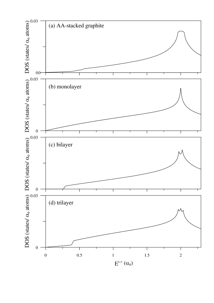
Figure 3: Optical absorption spectra of the AA-stacked (a) graphite, (b) monolayer, (c) bilayer, and (d) trilayer graphenes.

The 2D $\pi$-electronic structure of a monolayer graphene is reviewed first. Given the interlayer atomic interactions $\alpha_{1}=0$, $\alpha_{2}=0$ and $\alpha_{3}=0$ in Eq. (5), one can obtain the band structure of monolayer graphene, i.e., $E^{c,v}(k)=\pm\alpha_{0}|f(k_{x},k_{y})|=\pm\alpha_{0}\{1+4\cos(3bk_{x}/2\cos(\sqrt{3}bk_{y}/2+4\cos^{2}(\sqrt{3}bk_{y}/2\}^{1/2}$. The band structure is simplified as the projection of the energy dispersion of the simple hexagonal graphite on the $k_{z}=0$ plane (the red hexagon in Fig. 2(a)). Both conduction and valence bands are symmetric about the Fermi level ($E_{F}=0$) along K$\rightarrow\Gamma\rightarrow$ M$\rightarrow$K. In the low-energy region, the energy dispersion is described by $E^{c,v}=\pm 3\alpha_{0}bk/2$, which characterizes an isotropic Dirac cone centered at the K point (the Fermi level). There are special band structures at highly symmetric points in the 1st BZ, e.g., the local maximum $E^{c}=3\alpha_{0}$ and the local minimum $E^{v}=-3\alpha_{0}$ at the $\Gamma$ point, and the saddle points $E^{c,v}=\pm\alpha_{0}$ at the M point. Such critical points in the energy-wave-vector space would induce Van Hove singularities in DOS. The band width is evaluated as $6\alpha_{0}$, which is determined by the difference between the two local extreme values at the $\Gamma$ point. Monolayer graphene is a zero-gap semiconductor with a vanishing DOS at $E_{F}$ (Fig. 3(b)); that is, free carriers are absent at zero temperature.

The interlayer atomic interactions can dramatically change electronic structures. According to Eq. (5), the energy dispersions of simple hexagonal graphite without magnetic field are shown by the black curves in Fig. 2(a). There exists one pair of valence and conduction bands, in which the former is no longer symmetric to the latter about the Fermi level, $E_{F}=0.016$ eV. Energy bands are highly anisotropic and strongly dependent on $k_{z}$. At a fixed $k_{z}$, the $(k_{x},k_{y})$-dependent energy dispersions resemble those of a monolayer graphene. Moreover, the critical points are very sensitive to the change of $k_{z}$, e.g., those at the corners (K and H; Fig. 1(e)), the middle points between two corners (M and L); the centers of the ${k_{x}-k_{y}}$ plane ($\Gamma$ and A). The energy spacing of a monolayer-like band structure grows when $k_{z}$ moves from K to H. That is, the Dirac-cone structures could survive and remain similar in the increase/decrease of $k_{z}$. This will be directly reflected in the magnetic quantization. The middle points, which correspond to the saddle points with high DOS, are expected to present the strong absorption spectra. Overall, the $\pi$-electronic width is evaluated as the energy difference between the maximum energy at the $\Gamma$ point and the minimum energy at the A point: that is, $[2(\alpha_{1}+\alpha_{2})+3(\alpha_{0}+2\alpha_{3})]-[-2(\alpha_{1}-\alpha_{2})-3(\alpha_{0}-2\alpha_{3})=4\alpha_{1}+6\alpha_{0}$.

In the low-energy approximation around the corners along the K-H direction, Eq. (5), used to describe the Dirac-type energy dispersions, can be expressed as

$$E^{c,v}_{\pm}(k_{x},k_{y},k_{z})=E_{D}\pm v_{F}|\mathbf{k}|$$ (43)

where $E_{D}=\alpha_{1}h+2\alpha_{2}[h^{2}/2-1],v_{F}=3b(\alpha_{0}+\alpha_{3}h)/2$ (the Fermi velocity) and $|\mathbf{k}|=\sqrt{k_{x}^{2}+k_{y}^{2}}$. The first term $E_{D}$ indicates the Dirac-point energy. The second term represents the conical energy dispersion of which the slope particularly shows a slight discrepancy on $k_{z}$.

A closer examination is necessary to explore the dependence of the Dirac cone on $k_{z}$. Given by $E_{D}$ in Eq. (41), the localization of the Dirac point is described as a correspondence to the energy dispersion along the K-H line (indicated by the arrow in Fig. 2). In the vicinity of the zone corners, the conduction and valence Dirac cones overlap each other. At the K point, the state energy of the Dirac point, $2(\alpha_{1}+\alpha_{2})$, is higher than $E_{F}$. This indicates that the valence states between $E_{F}$ and the Dirac point are regarded as free holes in the low-lying valence bands. As the states gradually move away from K toward H, the carrier density of free holes decreases because the Dirac point gets lower. It is not until the Dirac point approaches the Fermi level that there are no free carriers. With a further increase of $k_{z}$ ($E_{D}<E_{F}$), the free carrier change into electrons, being determined by the Fermi level in the conduction Dirac cone. Its density reaches a maximum value at the H point. In short, it means that the interlayer atomic interactions induce free-hole (free-electron) pockets in the low-energy valence (conduction) bands near the K (H) point. Two kinds of free carriers have the same density. Furthermore, the Dirac points of cone structures are located at the corners of the 1st BZ during the variation of $k_{z}$ (Fig. 1(e)). These are expected to play an important role in the essential physical properties, e.g., optical properties, magneto-electronic and magneto-optical properties, electronic excitations, and transport properties.

In the case of 2D multi-layer AA-stacked graphene, there are $N$ pairs of valence and conduction Dirac cones, mainly owing to the highest stacking symmetry. For example, there are two and three pairs in bilayer and trilayer graphenes, respectively (Figs. 2(b)$\&$ 2(c)), in which the overlap of valence and conduction cones indicates the semimetallic behavior. The Dirac-cone structures, which are initiated from the K point, are almost symmetric about the Fermi level. The Dirac-point energies between ${-2\alpha_{1}}$ and ${2\alpha_{1}}$ are described by[171]

$$E_{D}=2\cos[j\pi/(N+1)]\alpha_{1},$$ (44)

in the low-energy approximation (ignoring $\alpha_{2}$ and $\alpha_{3}$), where $j=1,2,......N$. When $N$ is an odd number, the Dirac point of the middle cone structure touches with the Fermi level. With an increase of layer number, the multi cone structures are gradually evolved into a 3D one with a significant $k_{z}$-dependent band width. However, it might have certain important differences between the AA-stacked few-layer graphenes and graphite in the essential properties as a result of the confinement effect along the $z$-direction, e.g., the optical threshold frequency, DOS, and the features of magneto-absorption peaks.

On the experimental side, ARPES can directly identify the wave-vector-dependent energy bands. Using the high-resolution ARPES measurements, the dimension-created unusual electronic structures have been verified for the carbon-related systems with the hexagonal symmetry, including graphene nanoribbons, number- and stacking-dependent graphenes, and AB-stacked graphite. The confirmed characteristics cover the confinement-induced energy gap and 1D parabolic bands in finite-width nanoribbons,[133, 173] the Dirac-cone structure in monolayer graphene,[176, 174, 175] two/three pairs of linear bands in bilayer/trilayer AA stacking, [49, 50] two pairs of parabolic bands in bilayer AB stacking,[176, 177] the partially flat, sombrero-shaped and linear bands in tri-layer ABC stacking,[69] and the bilayer- and monolayer-like energy dispersions in Bernal graphite at the K and H points, respectively.[178, 179, 180, 181, 182] The 3D band structure of AA-stacked graphite is worthy of the detailed ARPES examinations, especially for the Dirac-cone structures and the saddle points along the K-H and M-L lines, respectively. Such measurements can determine the intralayer and interlayer hopping integrals and the significant effects due to them.

The primary characteristics of electronic structures directly reflect on DOS. The low-energy special structures in DOS are dominated by the stacking configuration or the interlayer atomic interactions. In the range of ${|E|\leq\,0.3}$ eV and ${B_{0}=0}$, simple hexagonal graphite presents a plateau structure centered about $E=0$ (the Fermi level), as shown in Fig. 3(a). This originates from the superposition of all $k_{z}$-dependent Dirac-cone structures with various disks in the $(k_{x},k_{y})$ plane. A finite DOS at ${E=0}$ clearly illustrates the semi-metallic behavior. DOS grows quickly in the increase of $E$. There exist two very cusp structures at the middle energies of $[-2(\alpha_{1}-\alpha_{2})+(\alpha_{0}-2\alpha_{3})]\leq E\leq[2(\alpha_{1}+\alpha_{2})+(\alpha_{0}+2\alpha_{3})]$ and $[-2(\alpha_{1}-\alpha_{2})-(\alpha_{0}-2\alpha_{3})]\leq E\leq[2(\alpha_{1}+\alpha_{2})-(\alpha_{0}+2\alpha_{3})]$ (Eq. (6)), mainly owing to the saddle points along the M-L line (Fig. 1(e)).[172] On the other hand, monolayer graphene exhibits a V-shape DOS near ${E=0}$, as shown in Fig. 3(b)). DOS vanishes at the Fermi level, leading to the semiconducting behavior. For N-even systems, the low-energy DOS corresponds to a plateau structure, e.g., that of bilayer graphene (Fig. 3(c)). However, it is a superposition of the plateau and V-shape structures for N-odd systems, such as DOS of trilayer graphene (Fig. 3(d)). Apparently, the AA-stacked graphenes of N${\geq\,2}$ belong to semimetals. At middle energy, the symmetric peaks of the logarithmic form mainly come from the saddle point (the M point in Figs. 2(a)-2(c)), in which their number is proportional to that of layer (Figs. 3(b)-3(d)).

3.2 Optical properties without external fields

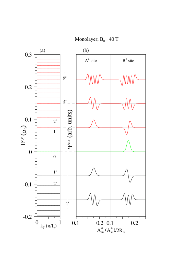
Figure 4: The Landau levels of monolayer graphene at ${B_{0}=40}$ T: (a) energy spectrum, and (b) amplitudes of subenvelope functions at two sublattices.

The main features of absorption spectra are determined by the velocity matrix element, carrier distribution and DOS. At low frequency, the first one is just the Fermi velocity in the AA stacking systems, mainly owing to the similar Dirac-cone with the isotropic linear dispersions.[172, 195] That is, the AA-stacked graphite and multi-layer graphenes have the identical excitation strength for each available channel. The former, as indicated in Fig. 4(a), presents a largely reduced low-frequency absorption spectrum and a shoulder structure at ${\omega\sim 4\alpha_{1}}$. For any given $k_{z}$, the vertical transitions are forbidden when half of excitation frequency is smaller than the energy difference ($E_{th}$) between the Fermi-momentum state ($\bf k_{F}$) and the Dirac point. $E_{th}$ is about $2\alpha_{1}$ for various $k_{z}$ s, so that absorption spectrum is very weak at $\omega\,<2\alpha_{1}$. With the increase of frequency, it exhibits a shoulder structure and grows quickly, since the deeper or higher electronic states make more contributions. On the other hand, absorption spectrum of monolayer graphene is linearly proportional to excitation frequency (Fig. 4(b)), directly reflecting the linear energy dependence of DOS (Fig. 3(b)). As for the middle-frequency absorption spectrum, graphite and graphene, respectively, exhibit the very prominent plateau and symmetric peak at ${2\alpha_{0}-4\alpha_{0}\leq\,\omega\leq\,2\alpha_{0}+4\alpha_{0}}$ and ${\omega\,=2\alpha_{0}}$. The former originates from the saddle points along the M-L line (Eq. (6)), with a rather high DOS. Such structures are the so-called $\pi$-electronic absorption peaks, frequently observed in the carbon-related systems with the sp² bondings (discussed later).

The AA-stacked layered graphenes present the unusual low-frequency absorption spectra during the variation of layer number, as clearly indicated in Fig. 4(b)-4(d). The critical factor is the well-behaved $N$ pairs of Dirac cones almost symmetric about the Fermi level.[195] The wave functions of these cone structures are the symmetric or anti-symmetric linear superposition of the layer-dependent tight-binding functions (e.g., Eq. (7)), leading to the available excitation channels only arising from the same Dirac cone. That is, the inter-Dirac-cone vertical transitions are absent. The $N$-odd systems have the zero threshold frequency, since the Dirac point of the middle cone structure touches with the Fermi level, e.g., the trilayer system (Fig. 4(d)). However, the optical gaps, which they are characterized the energy spacing of the highest occupied and the lowest unoccupied Dirac points (Eq. (42)), are finite in the N-even systems. They decline with the increasing layer number, and the highest threshold frequency is ${2\alpha_{1}}$ for the bilayer AA stacking (Fig. 4(c)).[58] As to the other intra-Dirac-cone excitations, their threshold spectra exhibit the shoulder structures with absorption frequency determined by the Fermi-momentum state (or about double that of energy difference between the Dirac point and the Fermi level). In addition, absorption spectra might reveal two sub-shoulders because of the slightly asymmetric Dirac-cone structures due to the interlayer atomic interactions, e.g., those of N=4 and 5ċiteAPL103;041907 Specifically, the change of layer number results in the crossing behavior. The AA-satcked graphenes and graphite possess the almost identical low-frequency optical properties when $N$ grows to 30 (detailed discussions in Ref.[195]) The dimension-induced important differences could be observed under the obvious confinement effect.

The above-mentioned features of vertical excitation spectra could be verified by optical spectroscopies, such as the absorption,[9, 10] transmission,[20, 9, 24, 23, 21] reflection,[87, 88, 9, 22] Raman scattering[216, 217, 218] and Rayleigh scattering spectroscopies.[237] Experimental measurements have confirmed the rich and diverse optical properties in the carbon-related systems, such as, Bernal graphite,[82, 83, 84, 85] graphite intercalation compounds,[202, 203] layered graphenes,[20, 21, 22, 23, 24] graphene nanoribbons,[156, 196] carbon nanotubes,[145, 146] and carbon fullerenes.[198, 197] Such systems possess the ${\sim 5-6}$ eV $\pi$ peak arising from the ${2p_{z}}$-orbital bondings; that is, all the ${sp^{2}}$-bonding systems can create this prominent peak. The AB- and ABC-stacked graphenes quite differ from each other in the absorption frequencies, spectral structures and electric-field-induced excitation spectra.[79, 80, 209, 230, 229] Moreover, carbon nanotubes exhibit the strong dependence of asymmetric absorption peaks on radius and chirality.[145] The important features in AA-satcked graphenes and graphite are worthy of systematic experimental investigations, especially for the dependence of optical gap, shoulder structure, $\pi$ peak, and spectral intensity on the layer number.

3.3 Magnetic quantization

3.3.1 Landau levels and wave functions

In the presence of $\mathbf{B}=B_{0}\hat{z}$, electrons are flocked on the $x-y$ plane to form the transverse cyclotron motions, while the motion along the field direction remains intact. The 3D electronic states in simple hexagonal graphite are evolved into one group of so-called LSs, which are dispersed along the $\widehat{k_{z}}$ direction, but highly degenerate on the $k_{x}-k_{y}$ plane. This implies that the $k_{z}$-dependent LSs are directly quantized from the corresponding $k_{z}$-dependent Dirac cones along K-H in the absence of a magnetic field. The study on the magnetic quantization of a Dirac cone in monolayer graphene is the first step to realize the magneto-electronic properties in graphites.

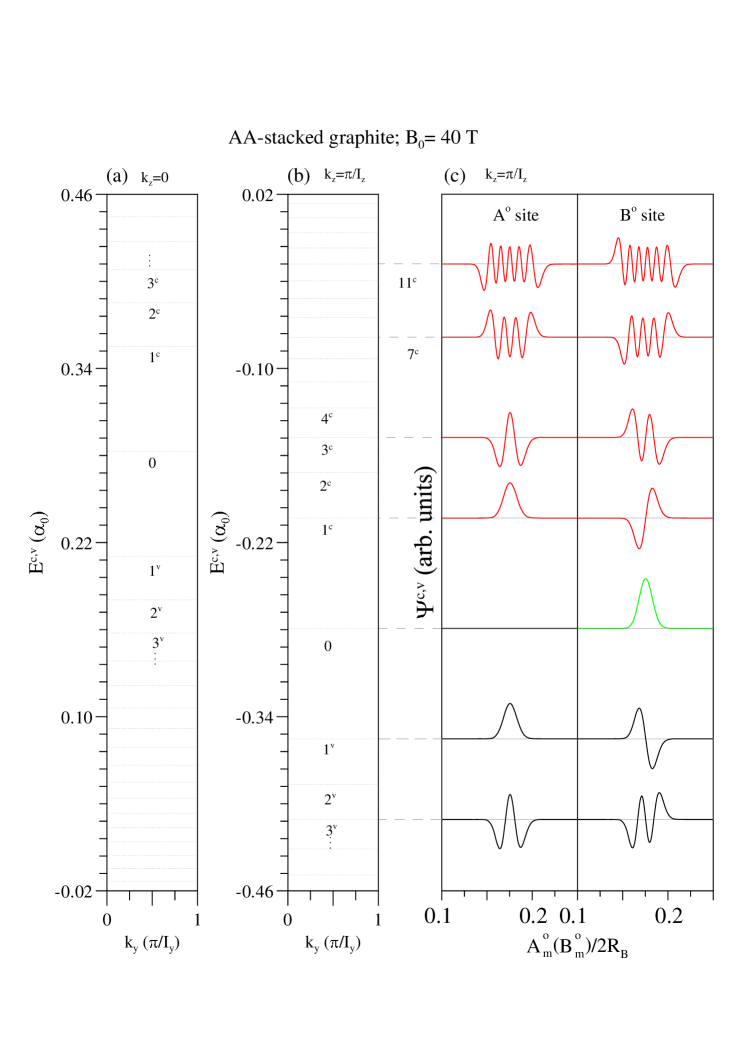
Figure 5: The Landau subbands of simple hexagonal graphite at ${B_{0}=40}$ T: energy spectrum corresponding (a) ${k_{z}=0}$ $\&$ (b) ${k_{z}=\pi\,/I_{z}}$, and (c) the amplitudes of subenvelope functions of the former.

The electronic states of a Dirac cone are magnetically quantized into one group of valence and conduction LLs. Each LL, dispersionless along $k_{x}$ and $k_{y}$, is fourfold degenerate without the consideration of spin degeneracy. The occupied valence and unoccupied conduction LLs are symmetric about $E_{F}=0$, as shown in Fig. 5 (a). The quantum numbers, characterized by the zero-point ones of the subenvelpe functions, are indicated by $n^{c}$ and $n^{v}$ for the conduction and valence LLs, respectively. Considering the sequence of LLs, one can find that the $n^{c,v}=0$ LLs are located at $E_{F}=0$, and the $n^{c,v}=1,2,3...$ LLs are counted away from the Fermi level (Fig. 4(a)). At ${(k_{x}=0,k_{y}=0)}$, the corresponding wave functions of the four-fold degenerate states are localized around four different centers: $1/6$, $2/6$, $4/6$ and $5/6$ positions of the enlarged unit cell. The main features of LLs can be realized by discussing one of the four-fold degenerate states, e.g., the $1/6$-localized Landau states (Fig. 5(b)). The quantum number is determined by the normal mode in $B_{o}$ sublattice. For the cases of $n^{c,v}\geq 1$ LL, the subenvelope functions of $A_{o}$ and $B_{o}$ sublattices are presented in the (${n^{c,v}-1}$)-th and an $(n^{c,v})$-th order Hermite polynomials, respectively. They have the following relationship between conduction and valence states: $A_{o}^{c}=A_{o}^{v}$ $\&$ $B_{o}^{c}=-B_{o}^{v}$ for the same atoms, and $A_{o}^{v}(n^{v})\propto B_{o}^{c}(n^{c}=n^{v}-1)$ $\&$ $B_{o}^{v}(n^{v})\propto A_{o}^{c}(n^{c}=n^{v}+1)$ for the different atoms. It can be deduced that as to the inter-LL optical transitions, the simple linear relationships account for the specific selection rule $\Delta n=n^{c}-n^{v}=\pm 1$, according to the spectral function in Eq. (38).

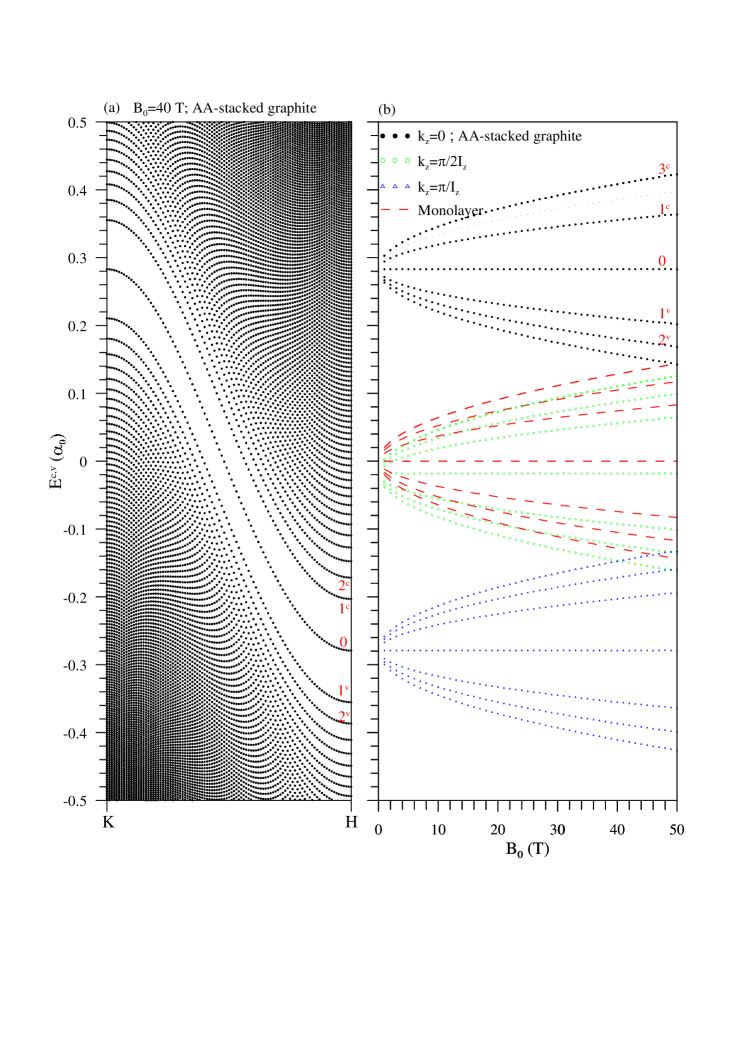
Figure 6: The LS energy spectra of the AA-stacked graphite (a) along the KH dircetion at ${B_{0}=40}$ T and (b) for the $B_{0}$-dependence at various $k_{z}$s. Also shown in (b) is that of monolayer graphene.

For simple hexagonal graphite, the formation of the LSs corresponds to the magnetic quantization of the Dirac cones that are distributed along the K-H line as described by Eq. (41). The LS energy dispersions strongly depend on $k_{z}$, and the relationship between Landau states and wave functions at a fixed $k_{z}$ resembles that of a monolayer graphene. These purely arise from the highly symmetric AA stacking with the same ${(x,y)}$-plane projection. At the K point, the conduction and valence LLs are symmetric about $E^{c,v}(n^{c,v}=0,k_{z}=0)=E_{D}(k_{z}=0)\simeq 0.283\alpha_{0}$, as indicated in Fig. 6(a). The similar LL spectrum is revealed at the H point, while it is centered about $E_{D}(k_{z}=\pi/I_{z})$$\simeq-0.279\alpha_{0}$ (Fig. 6(b)). With the same quantum number, the AA-stacked graphite and monolayer graphene have the same relationship of two subenvelope functions with respect to the amplitude, spatial symmetry, phase and zero points, as shown in Figs. 6(c) and 5(b). Moreover, the linear relationship between two subenvelope functions remains the same, clearly illustrating that the specific optical selection rule of $\Delta n=\pm 1$ is also applicable to the inter-LS transitions in simple hexagonal graphite. In short, 3D simple hexagonal graphite consisting of the same projection graphenes layers exhibits the essential 2D quantum phenomena, mainly owing to the Dirac-type energy dispersions.

3.3.2 Landau subband energy spectra

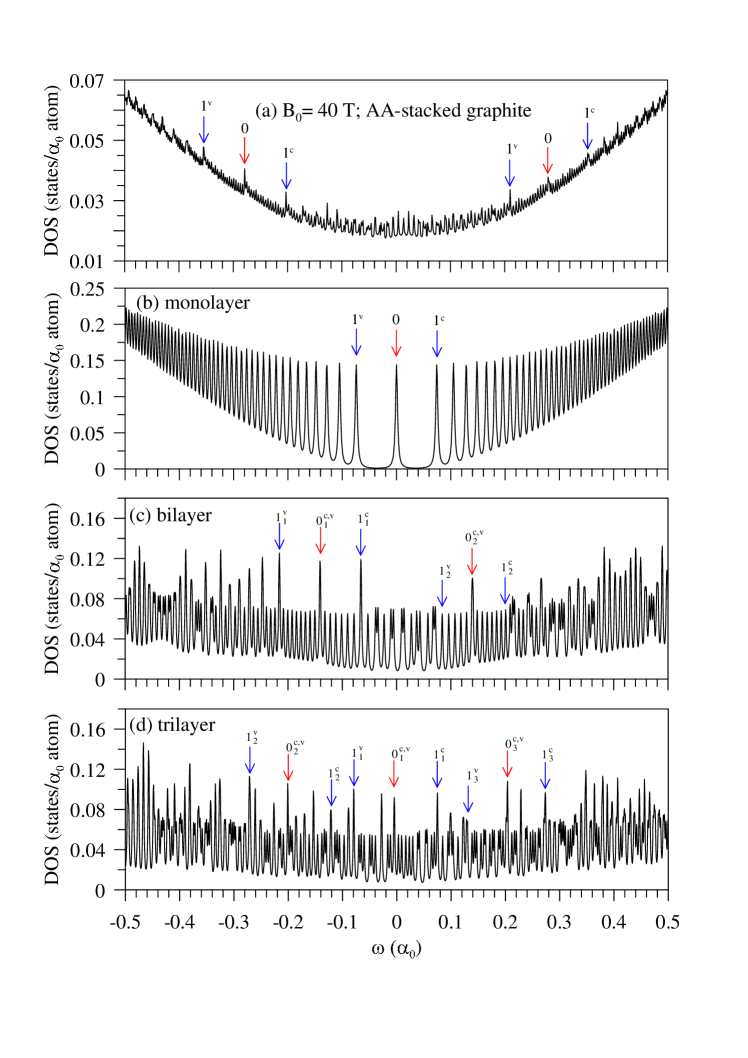
Figure 7: Magneto-electronic density of states at ${B_{0}=40}$ T for (a) simple hexagonal graphite, and (b) monolayer, (c) bilayer and (d) trilayer graphenes.

The LS spectrum in the 1st BZ ($0\leq k_{z}\leq\pi/I_{z}$) is essential for understanding the magneto-electronic properties of bulk graphites. In the K-H direction, the LSs at a fixed $B_{0}$ exhibit a parabolic dispersion with two band-edge states at the two edges of the 1st BZ, i.e., K ($k_{z}=0$) and H ($k_{z}=\pi/I_{z}$), as shown for $B_{0}=40$ T in Fig. 7 (a). There are no crossings and anticrossings of LSs, directly reflecting the monotonous dependence of energy bands on wave vectors (the black curve in Fig. 2 (a)). In particular, the $k_{z}$-dependent dispersion of the $n^{c,v}=0$ LS is consistent with that of the Dirac points along the K-H direction in the absence of external fields, i.e., ${E^{c,v}(n^{c,v}=0,k_{z})=E_{D}(k_{z})}$. A slice of the LS spectrum with respect to a specific $k_{z}$ can be regarded as a combination of massless-Dirac LLs with the zeroth LL given by $E_{D}(k_{z})$. Furthermore, according to Eq. (41), the energy width of a LS corresponds to the energy difference between the Dirac points at the zone edges, K and H: that is, $E_{D}(k_{z}=0)-E_{D}(k_{z}=\pi/I_{z})=(2\alpha_{1}+2\alpha_{2})-(2\alpha_{1}\cos(\pi)+2\alpha_{2}\cos(2\pi))=4\alpha_{1}\simeq 1.444$ eV. It should be noticed that simple hexagonal graphite retains the semi-metallic characteristics in the presence of a magnetic field, implying that free carrier pockets near the K-H edge might cause the optical transitions between two valence or conduction LSs (intraband excitations).

On the other hand, with the variation of $B_{0}$, the field-dependent energy spectrum displays a form similar to that of monolayer graphene, ${E^{c,v}(n^{c,v},k_{z})-E_{D}(k_{z})}\propto\sqrt{n^{c,v}B_{0}}$, while the proportional constant ($\propto$ the Fermi velocity) is weakly dependent on $k_{z}$, as shown in Fig. 7 (b). In the low-energy approximation, the analytic solution of LS energies is derived by introducing the quantization condition to the Dirac cone of graphites as in Eq. (41) to have

$$\begin{gathered}E^{c,v}(n^{c,v},k_{z})\approx E_{D}(k_{z})\pm\hbar v_{F}\sqrt{2eB_{0}n^{c,v}/\hbar}.\end{gathered}$$ (45)

By the detailed calculations, the four atomic interactions, $\alpha_{0},\alpha_{1},\alpha_{2}$ and $\alpha_{3}$, can be expressed in terms of the low-lying LS energies at the K and H points as follows:

$$\begin{gathered}\alpha_{0}=\frac{l_{B}}{3\sqrt{2}b}\{E^{c}(n^{c}=1,k_{z}=0)-E^{c,v}(n^{c,v}=0,k_{z}=0)\\ +E^{c}(n^{c}=1,k_{z}=\pi/I_{z})-E^{c,v}(n^{c,v}=0,k_{z}=\pi/I_{z})\},\\ \alpha_{1}=\frac{1}{4}\{E^{c,v}(n^{c,v}=0,k_{z}=0)-E^{c,v}(n^{c,v}=0,k_{z}=\pi/I_{z})\},\\ \alpha_{2}=\frac{1}{4}\{E^{c,v}(n^{c,v}=0,k_{z}=0)+E^{c,v}(n^{c,v}=0,k_{z}=\pi/I_{z})\};\\ \alpha_{3}=\frac{l_{B}}{6\sqrt{2}b}\{E^{c,v}(n^{c}=1,k_{z}=0)-E^{c,v}(n^{c,v}=0,k_{z}=0)\\ -E^{c}(n^{c}=1,k_{z}=\pi/I_{z})+E^{c,v}(n^{c,v}=0,k_{z}=\pi/I_{z})\}.\end{gathered}$$ (46)

${l_{B}=\sqrt{\hbar c/eB_{0}}}$ is the magneto length related to the effective localization range of LS. Equation (44) means that the atomic interactions can be determined by the STS and magneto-optical measurements on the LS energies. Based on the band structure, 3D graphite is expected to display the massless Dirac-like magneto-optical properties. However, as a result of the strongly dispersed LSs across the Fermi level, the greatly enhanced free carrier pockets near the edges of the first Brillouin zone is responsible for the spectral features that are considerably differ from the essential quantum phenomena in 2D graphenes.

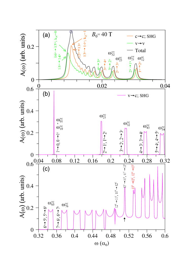
Figure 8: Magneto-optical absorption spectrum of simple hexagonal graphite in (a) to (c) within different frequency ranges at ${B_{0}=40}$ T.

The magnetically quantized DOS has a lot of special structures, depending on 1D LSs or 0D LLs. Simple hexagonal graphite exhibits many peaks in the square-root form arising from the quantized LSs with the 1D parabolic dispersions, as shown in Fig. 8(a). Each LS contributes two asymmetric peaks corresponding to the band-edge states at the K and H points. For example, at $B_{0}=40$ T, the $n^{c,v}=0$ ($n^{c}=1$) LS has two peaks at $E=0.272\alpha_{0}$ and $-0.272\alpha_{0}$ ($E=0.35\alpha_{0}$ and $-0.195\alpha_{0}$), as indicated by the red (blue) arrows. On the other hand, few-layer graphenes present a plenty of delta-function-like symmetric peaks due to the dispersionless LLs, e.g., monolayer, bilayer and trilayer systems in Figs. 8(b)-8(c), respectively. The initial peak of the zeroth mode (the red arrows) corresponds to the Dirac point (Figs. 2(b)-2(d)).

STS is an efficient method in examining energy spectra of condensed-matter systems. The tunneling differential conductance (dI/dV) is approximately proportional to DOS and directly presents the main features in DOS. The STS measurements have been successfully utilized to identify the diverse electronic properties in graphene-related systems with the $sp^{2}$ bondings, such as, few-layer graphenes,[183, 184, 185, 117, 66, 186, 187, 118] Bernal graphite,[188, 189] graphene nanoribbons,[190, 191, 192] and carbon nanotubes.[193, 194] Specifically, two low-lying DOS characteristics, a linear $E$-dependence vanishing at the Dirac point and a ${\sqrt{B}_{0}}$-form LL energy spacing, are confirmed for monolayer graphene.[183, 184, 76, 77] A sufficient-wide plateau and a lot of square-root LS peaks in AA-stacked graphite require further experimental verifications. The STS measurements on them are useful in the identifications of the intralayer and interlayer atomic interactions.

3.4 Magneto-optical properties

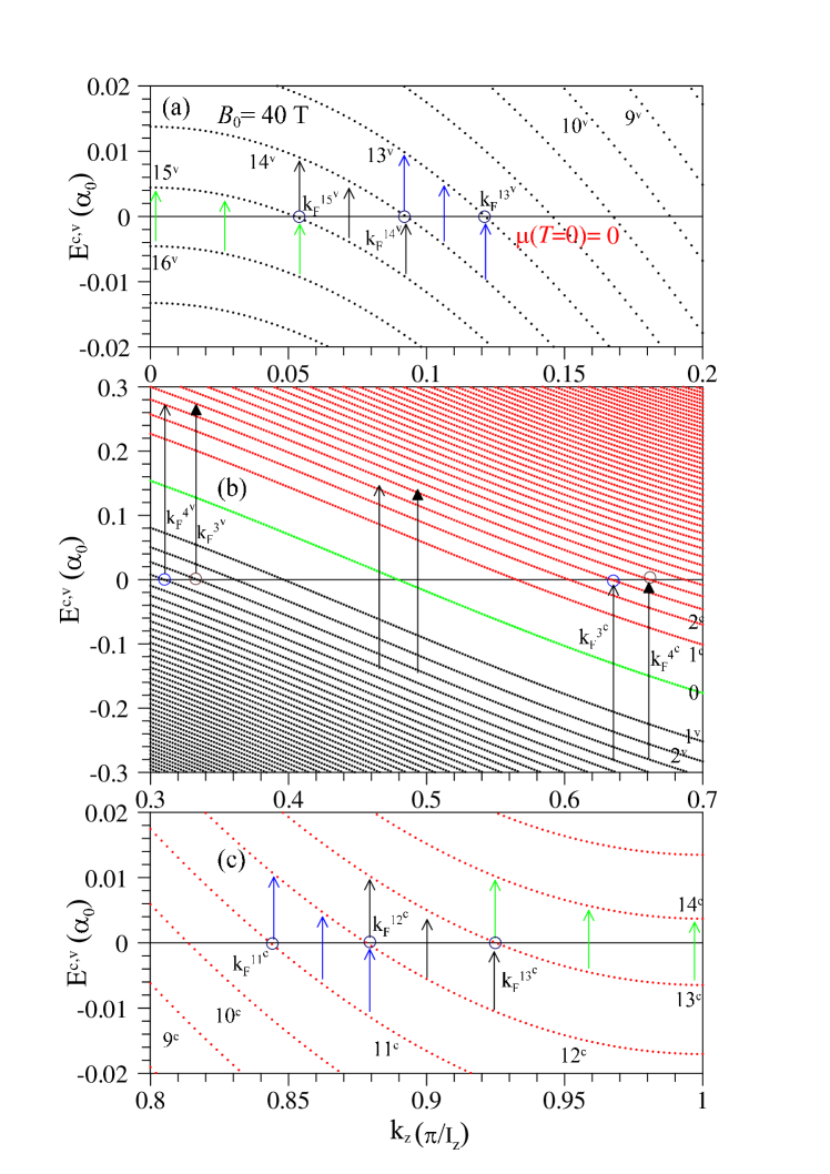
Figure 9: Vertical optical transitions due to the Landau subbands near (a) ${k_{z}=0}$, (b) ${k_{z}=\pi\,/2I_{z}}$, and (c) ${k_{z}=\pi\,/I_{z}}$.

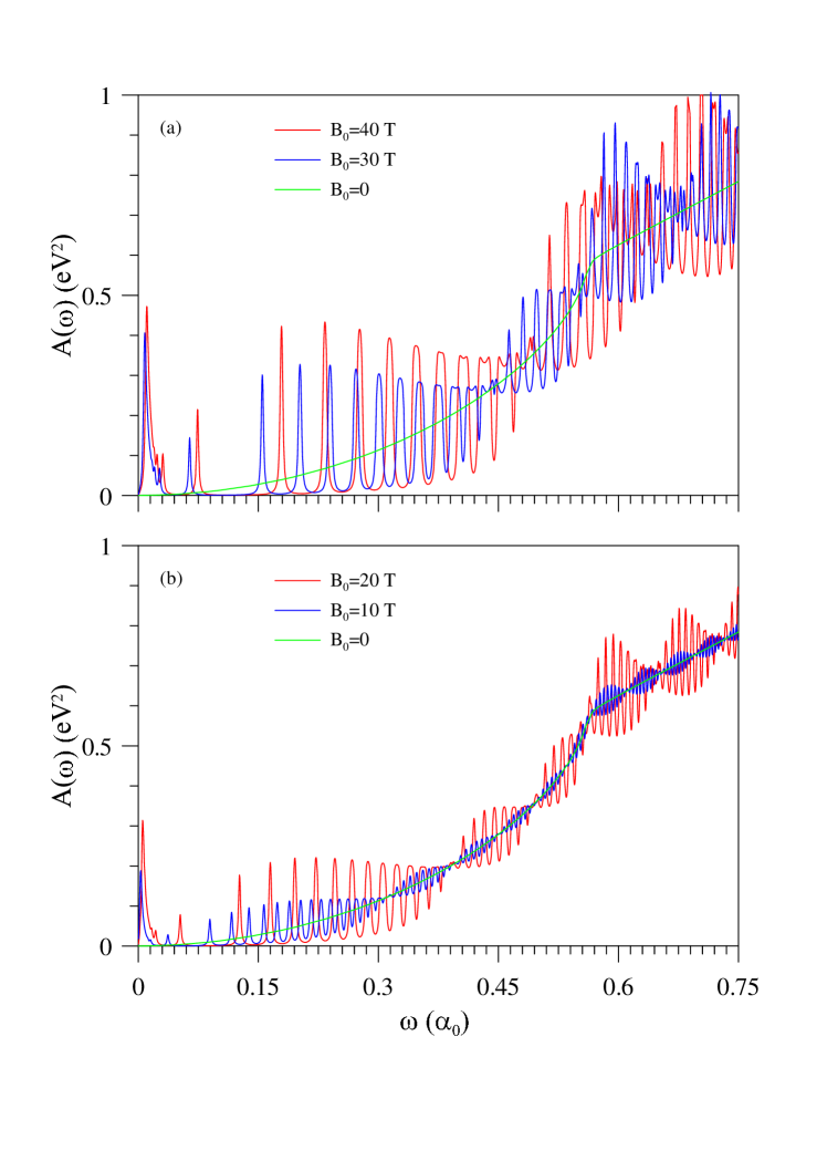
Figure 10: The beating magneto-absorption spectra of simple hexagonal graphite for various field strengths in (a) and (b).

The AA-stacked graphite exhibits the unique magneto-optical properties, since the 1D LSs have the sufficiently wide band widths and the specific energy dispersions. The intraband and the interband inter-LS vertical excitations appear in the low-frequency absorption spectra, as clearly indicated in Figs. 9(a)-9(c).[56] The former originate from the valence and conduction LSs across the Fermi level. Only the occupied $n^{v}$ ($n^{c}$) LS to the unoccupied ${n^{v}-1}$ (${n^{c}+1}$) one is the effective excitation channel; that is, the optical excitations between the well-behaved Landau wavefunctions need to satisfy the selection rule of ${\Delta\,n=\pm\,1}$. The intraband absorption peaks are denoted as ${\omega^{vv}_{nn-1}}$ and ${\omega^{cc}_{nn+1}}$ (Fig. 9(a)). They are closely related to the $k_{z}$-dependent Fermi-momentum state of each LS ($k_{F}^{n^{c,v}}$ in Figs. 10(a) and 10(c)). For example, the ${\omega_{1615}^{vv}}$ peak comes from all the vertical excitations in the range of ${k_{F}^{16^{v}}\leq\,k_{z}\leq\,k_{F}^{15^{v}}}$ (Fig. 10(a)). ${\omega^{vv}_{n+1n}}$ is close to ${\omega^{cc}_{nn+1}}$, so their absorption peaks are merged together, e.g., those for ${n^{v}\leq\,15}$ and ${n^{c}\leq\,14}$ at ${B_{0}=40}$ T (Fig. 9(a)). Such two-channel peaks are observable for ${n^{c,v}\leq\,6}$. As a result of the smaller frequency differences, the other peaks become a broad and prominent structure, i.e., they behave as a multi-channel threshold peak. This composite structure is absent in the layered graphenes and other graphites.

The interband absorption peaks come to exist in the frequency range of ${\omega\,>}0.039\alpha_{0}$, as clearly shown in Fig. 9(b). They originate from the ${(n+1)^{v}\rightarrow\,n^{c}}$ and ${n^{v}\rightarrow\,(n+1)^{c}}$ vertical excitations, respectively, corresponding to the allowed ranges in ${k_{F}^{(n+1)^{v}}\leq\,k_{z}\leq\,k_{F}^{n^{c}}}$ and ${k_{F}^{n^{v}}\leq\,k_{z}\leq\,k_{F}^{(n+1)^{c}}}$. ${k_{F}^{n^{c}}-k_{F}^{(n+1)^{v}}}$ is almost identical to ${k_{F}^{(n+1)^{c}}-k_{F}^{n^{v}}}$, and corresponding excitation frequencies behave similarly (Fig. 10(b)). Two kinds of interband channels can create nearly the same absorption spectrum. The effective $k_{z}$-ranges are sufficient wide except for very small quantum numbers, so that the distinct curvature variations of the ${(n+1)^{v}}$ and ${n^{c}}$ LSs result in two specific absorption frequencies due to the Fermi-momentum states ${k_{F}^{(n+1)^{v}}}$ and ${k_{F}^{n^{c}}}$. Furthermore, such ranges cover the ${k_{z}=\pi\,/2I_{z}}$ state with the lowest DOS. These are responsible for the existence of many double-peak structures in the cusp form. Such double peaks have the non-uniform intensity, and their widths grow with the increasing frequency because of the enlarged range between two associated Fermi-momentum states.

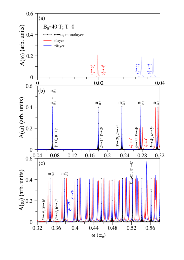
Figure 11: Magneto-optical absorption spectra of monolayer, bilayer and trilayer graphenes in (a) to (c) within different frequency ranges at ${B_{0}=40}$ T.

The interband magneto-absorption spectra present the unique beating phenomena, as clearly indicated in Figs. 11(a)-11(b). The beating oscillations, which include several groups of diversified absorption peaks, are very sensitive to the change of field strength. With the increase of absorption frequency, the widened double-peak structures might overlap each other or one another. The first group at lower frequency is composed of the isolated double peaks. The second group arises from a combination of two neighboring double peaks, and their composite peak intensity is twice that of the original peaks. Concerning the third group, three neighboring peaks are merged to a single structure and its intensity is enhanced to almost three times the pristine one. As a result, the spectral intensity is proportional to the number of the combined double-peak structures. The unusual association of absorption peaks directly reflects the specific $k_{z}$-dependence of each LS parabolic dispersion (Eq. (43); details in [57]). It should be noticed that this is the first time to predict the beating phenomenon in optical properties.

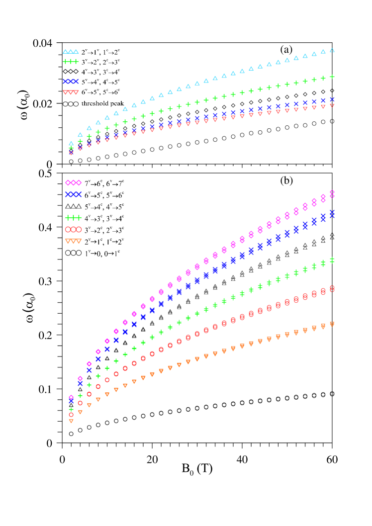
Figure 12: The $B_{0}$-dependent absorption frequencies of simple hexagonal graphite corresponding to (a) intraband and (b) interband excitation channels.

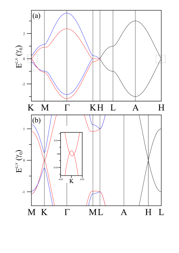
Figure 14: Band structures for AB-stacked (a) graphite and (b) the zoomed-in view at low energies near the K and H points.

The magneto-absorption peaks of few-layer graphenes and graphite, with the exception of the optical selection rule ${\triangle\,n=\pm\,1}$, reveal very distinct features. For the former, the dispersionless LLs create the delta-function-like symmetric structures with a uniform intensity, as shown in Figs. 12(a). The multi-channel threshold peak is absent. Only one two-channel peak, belonging to the intraband absorption channel, is present in bilayer and tri-layer AA stackings (red and blue curves in Fig. 12(a)), in which it does not have a complete dispersion relation with the $B_{0}$-field strength because of the variation of the highest occupied LL (Fig. 14(b) and (d)).[55] All the AA-stacked systems exhibit a plenty of interband absorption peaks, but the main differences lie in the peak structures. Monolayer system shows the isolated symmetric peaks, while bilayer AA stacking displays the pair-peak structures. Furthermore, the N-odd systems correspond to the superposition of the monolayer- and bilayer-like absorption peaks. Some initial ${n^{v}\rightarrow\,n^{c}}$ excitations are forbidden in N=2 ${\&}$ 3 systems, reflecting the Fermi-Dirac distribution of multi-Dirac ones. In addition, the well-behaved beating oscillations are not presented in layered graphenes.

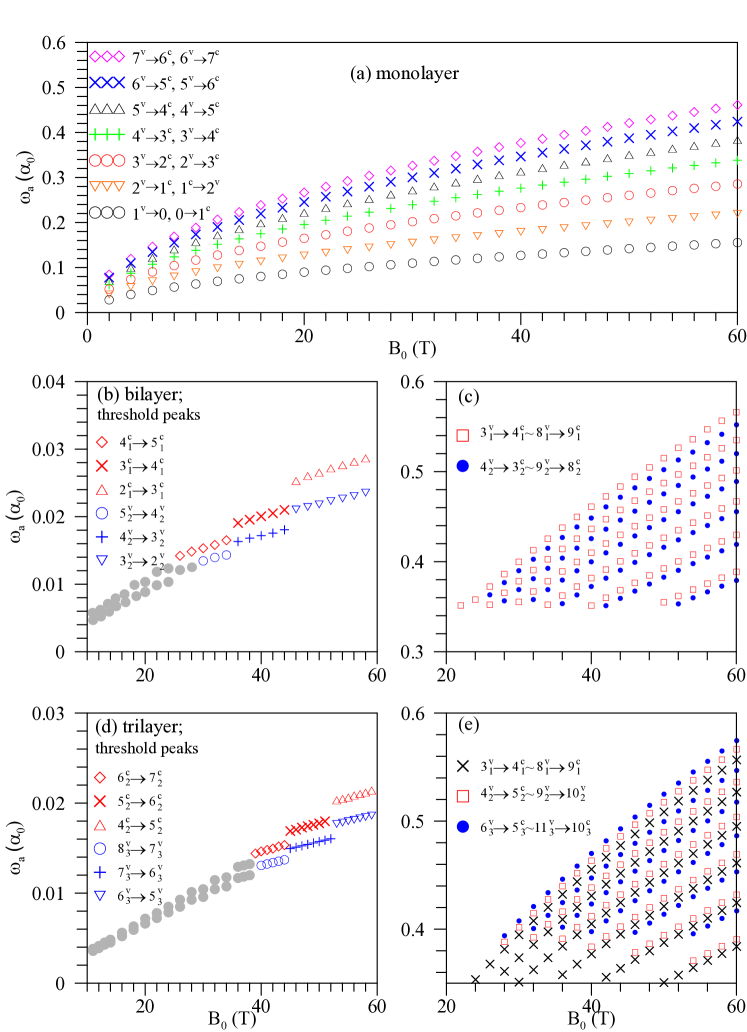
Figure 13: The magneto-absorption frequencies for (a) monolayer, (b)-(c) bilayer and (d)-(e) trilayer graphenes. The discontinuous $B_{0}$-dependence of the threshold channel is shown in (b) and (d).

The $B_{0}$-dependent absorption frequencies provide the important information for the experimental verifications and in understanding the effects due to dimensions and stacking configurations. All peak frequencies of AA-stacked graphite, as shown in Figs. 13(a) and 13(b), grows with an increasing field strength. They present the complete dispersion relations with $B_{0}$, in which the field-strength dependence is roughly proportional to ${\sqrt{B}_{0}}$ except for the multi-channel peak (solid circles in Fig. 13 (a)). The observable intraband excitations cover the multi-channel peak and five two-channel peaks. The multi-channel threshold frequency does not exhibit a ${\sqrt{B}_{0}}$-dependence, since the initial intraband excitation channels dramatically change with field strength. Concerning the interband excitations, there exist two splitting absorption frequencies at sufficiently high magnetic field. The critical field strength is reduced in the higher-frequency absorption peaks. It is relatively easy to observe the double-peak structures for large $\omega$ and ${B_{0}}$. On the other side, the layered graphenes exhibit the unique intraband and interband absorption frequencies, as clearly indicated in Figs. 14(a)-14(e). Monolayer graphene has a regular ${\sqrt{B}_{0}}$-dependence at low magneto-absorption frequency (${\omega\,<1}$ eV in Fig. 14(a)). As to bilayer and trilayer AA stackings, they show the discontinuous $B_{0}$-dependences in the two-channel intraband peaks (Figs. 14(b) and 14(d)). This mainly stems from the fact that the highest occupied LL becomes the smaller-$n^{c,v}$ one in the increase of $B_{0}$. Furthermore, their pair-peak interband excitations cannot survive when both $n^{v}$ and ${(n+1)^{c}}$ are occupied or unoccupied, i.e., more interband absorption peaks are absent at low field strength (Figs. 14(c) and 14(e)). In addition, the critical differences among three kinds of graphites will be discussed in Chap. 6.

As for magneto-optical measurements, the infrared transmission spectra have identified the ${\sqrt{B}_{0}}$-dependent absorption frequencies of the interband LL transitions in mono- and multi- graphene.[21, 85, 23, 24] Furthermore, the magneto-Raman spectroscopy is utilized to observe the low-frequency LL excitation spectra for the AB-stacked graphenes up to 5 layers.[216] The unique magneto-excitation spectra of simple hexagonal graphite deserve thorough experimental examinations, such as, the multi-channel threshold peak, the intraband two-channel peaks, the interband double-peak structures, and the magneto-optical beating phenomenon. Similar measurements could be done for AA-stacked graphenes to verify the dimension-induced differences in the channel, structure, number, frequency and intensity of magneto-absorption peaks. Such comparisons are useful in illustrating the diversified magnetic quantization of the multiple Dirac-cone structures in the AA stacking systems.

4 Bernal graphite

Bernal graphite, with band profiles of monolayer and bilayer graphenes, is a critical bulk material for a detailed inspection of the massless and massive Dirac fermions. Theoretical and experimental researches show that the essential properties of graphite can be described by the quisiparticles at the high symmetry points of the Brillouin zone: massless Dirac fermions at the H point and massless ones at the K point. In particular, with the dimensional crossover from 3D to 2D, the many exciting properties of fewlayer graphenes originate from the interlayer couplings in bulk graphite. The optical excitation channels are only allowed between the respective monolayer-like subbands or between the bilayer-like subbands, regardless of external fields. The anticrossings of LLs/LSs and the electron-hole induced twin-peak structures are revealed in both 2D graphene and 3D graphite, while they are are more obvious in graphene with the increase of the layer number.

are crucially massive Dirac fermions dependent on understanding the interlayer coupling that originates in bulk graphite.

However, based on the interlayer atomic interactions of the dimensional crossover, the measured profiles of the B0-dependent peaks, e.g., threshold channels and peak intensity, spacing and frequency, can be used to distinguish the stacking layer, configuration and dimensionality.

4.1 Electronic structures without external fields

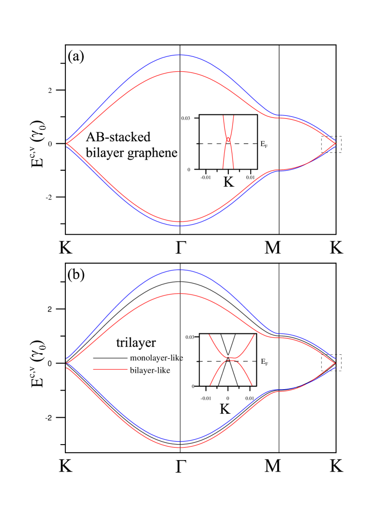
Figure 15: Band structures of AB-stacked (a) bilayer and (b) trilayer graphenes.

The band structure of the Bernal graphite in the absence of external fields are shown in Figs. 15 (a) and (b). With a slight overlap of conduction and valence subbands, Bernal graphite is classified as a semimetal due to the low-density free carriers. The in-plane energy dispersions considerably depends on the value of the momentum $k_{z}$, which contain the characteristics of 2D monolayer and AB-stacked bilayer graphenes at certain special $k_{z}$’s. In Eq. (11), $h=2\cos(k_{z}I_{z})$ indicates the factor of the effective interlayer interactions in Bernal graphite. In the HLA plane ($k_{z}=\pi/2I_{z}$ and $h=2\cos(\pi/2)=0$), the Hamiltonian matrix can be reduced to a $2\times 2$ matrix of monolayer graphene, because the elements coupling by the nearest-layer interactions are equal to zero and the on-site energy $\gamma_{6}$ can be negligible. It is shown that the occupied valence bands $E_{v}$ are symmetric to the unoccupied conduction bands $E_{c}$ about $E_{F}=0$ (Fig. 15 (b)). The low-energy band structure displays a massless-Dirac-like linear dispersion with the Dirac point located near the H point, while the energy states are double degenerate.

The energy dispersions in the M$\Gamma$K plane show another graphene properties. Substituting the condition $k_{z}=0$ and $h=2\cos(0)=2$ into the Hamiltonian matrix in Eq. (11), one gets a $4\times 4$ bilayer-like Hamiltonian matrix, while the effective interlayer interactions are twice as large as those of bilayer graphene. The in-plane energy subbands are asymmetric about the Fermi level due to the influence of the interlayer atomic interactions, $\gamma_{2}$,…$\gamma_{6}$. In the vicinity of the K point, the low-energy dispersions are characterized by massive-Dirac quasi-particles. The coordinate of the band-edge states are consistent with those of AB-stacked bilayer graphene, i.e., at the M and K points. However, the effective interlayer atomic interaction 2$\gamma_{1}$ gives rise to the double band-edge state energies $\sim 2\gamma_{1}$ at the K point as compared to the bilayer graphene.

Along KH, the strongly anisotropic energy dispersions on $k_{z}$ are mainly caused by the interlayer interactions. The cosine and the flat dispersions along KH (Fig. 15(a)) are responsible for the two types of atom chains; one is a straight chain of sublattices coupled by $\gamma_{1}$ along $\widehat{z}$, and the other is a zigzag chain of sublattices coupled by $\gamma_{4}$ in the $yz$-plane. In the minimum model, the former and the latter are, respectively, described by $E^{c,v}\simeq\gamma_{1}h=2\gamma_{1}\cos(k_{z}I_{z})$ and $E^{c,v}\simeq 0$.[93] When the state grows from K($k_{z}=0$) to H($k_{z}=\pi/2I_{z}$), the two dispersions gradually get closer and become degenerate at the H point. Also, the in-plane dispersions are bilayer-like, while their behavior transforms into monolayer-like at the H point. That is to say, Beranl graphite exhibits both the massless and massive Dirac fermions in the vicinity of the H and K points, respectively. ARPES has been used to measure the 3D energy dispersions all around the 1st BZ from the hole pocket at the H point to the electron pocket at the K point. [178, 179, 180, 181, 182]. Both the massless and massive Dirac fermions are verified in terms of the linear and parabolic dispersions, respectively. Furthermore, the measured small hole pocket at the H point is in agreement with the theoretical model and the quantum oscillation measurements.[199] Remarkably, the Dirac quasi-particles are responsible for special structures in the DOS and dominate the optical excitations.

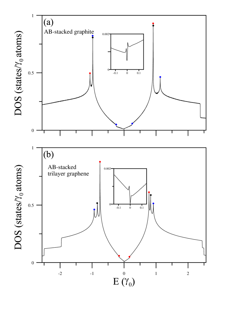
Figure 16: The DOS of AB-stacked (a) graphite and (b) trilayer graphenes.

On the other hand, N-layer AB-stacked graphenes could exhibit massless and massive Dirac fermions; the band structure resembles bilayer case or a hybridization of monolayer and bilayer cases, depending on whether the layer number is odd or even. The trilayer graphene displays a hybridization of band structure by a monolayer and a bilayer graphenes, while the even-layer graphene consist of only pairs of bilayer-like parabolic subbands, as shown in Fig. 16. Near the K point, the intersection of low-energy subbands indicates that AB-stacked graphenes are gapless 2D semimetals (the insets of Figs. 16 (a) and (b)). With an increment of the graphene layer, the band structure in cases of even (odd) N consists of N (N-1) pairs of bilayer-like parabolic bands, while it owns a particular pair of monolayer-like linear bands near the Fermi level if N is odd.

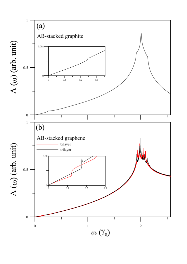
Figure 17: Optical absorption spectra of Bernal (a) graphite and (b) graphene.

The main characteristics of electronic structures, dominated by the stacking configuration or the interlayer atomic interactions, are directly reflected in the DOS. In Beranl graphite, the DOS mainly originates from the bilayer-like and monolayer-like in-plane dispersions, respectively, corresponding to the K- and H-point band-edge along the $k_{z}$ dispersions (Fig. 17). The DOS VHSs marked by black, red and blue colors correspond to the band-edge and saddle-point states in Figs. 15 and 16. A finite DOS at $E=0$ clearly indicates its semi-metallic properties of Bernal graphite. Besides, the low-energy intensity smoothly grows with the frequencies, which can be regarded as a superposition of the linear and pearabolic dispersions. The former and the latter are, respectively, verified in DOS by the roughly linear and quadratic $B_{0}$-dependent tunneling energies.[186] However, a shoulder spreads out near $\pm 2\gamma_{1}$, attributed to the band-edge states of bilayer-like parabolic subbands. Such structure is reflected by a VHS at $\sim\pm\gamma_{1}$ in bilayer and trilayer graphenes.[66] With the increasing energies, the DOS exhibits two prominent asymmetric peaks at the middle energies of $E^{c,v}\simeq\pm\gamma_{0}$. This is a superposition of all saddle points distributed along M$\rightarrow$L during the band structure transformation from bilayer-like to monolayer-like. In contrast, the trilayer graphene display three prominent peaks: one comes from band-edge state of monolayer-like subband and two from those of bilayer-like ones. Some of the main features in DOS are verified by STS[66, 186] and the measured VHSs could lead to special structures in absorption spectra.

4.2 Optical properties without external fields

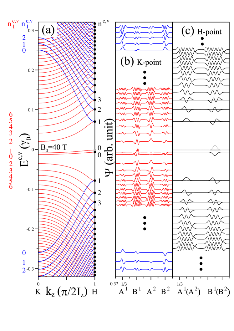
Figure 18: (a) Landau subbands of Bernal graphite. The subenvelope functions are shown for the (b) K and (c) H points.

The absorption is determined by the relationship between the electronic structures (or DOS) and the optical excitation transitions. In Beranl graphite, it demonstrates that $A(\omega)$ is identical for all polarization directions, $\widehat{E}$, on the graphene plane, indicating the isotropy of the frequency distribution of the absorption intensity over all frequencies. The optical responses due to massless and massive Dirac fermions are, respectively, reflected by the optical excitations channels in the vicinity of the H and K points, as shown in Fig. 18 (a). At low energies, one weak shoulder is revealed at $E\simeq 2\gamma_{1}$ as a result of the excitations between the two low-energy parabolic bands. Moreover, at middle energies, a single sharp peak is accompanied by two shoulder on its both sides. They are responsible for the multi saddle-point channels of all the bilayer-like and monolayer-like band structures as $k_{z}$ moves from M to L.

Some of the features of the optical spectrum are consistent with the experimental results. In the study by Obraztsov et al.[201], they study the optical spectra of polarized beam in cases of the different polarizations on the graphene plane and the stacking direction, which are, respectively, indicated by p-polarized and s-polarized. All the cases show a similar behavior between the spectral intensity and polarization of the laser beam, while the photoresponse for p-polarized excitation beam is relatively strong than for the s-polarized one because of the relatively strong energy dispersions on the in-plane direction. The results might reflect the relatively strong energy dispersions for the in-plane direction than for the out-plane direction.

The optical response of the Dirac quasi-particles is also a dominant contributor for 2D AB-stacked graphenes. It leads to two kinds of special structures: discontinuities at low frequencies and logarithmic divergences at middle frequencies. The former and the latter, respectively, come from the vertical transitions around the K point and those around the M point, as shown by Fig. 18 (b). For the bilayer case, the absorption spectrum exhibits a single shoulder at $\omega\simeq\gamma_{1}$ and four peaks at $\omega\simeq 2\gamma_{0}$. Infrared spectroscopy have shown a clear picture for the low-energy excitations around the K point.[214, 213] Besides, the spectral intensity grows with the higher frequency, until in the middle-frequency spectrum, four logarithmic saddle-point peaks spread around $\omega\simeq 2\gamma_{0}$. On the other hand, the excitation channels of the trilayer graphene are only allowed between the respective monolayer-like subbands or between the bilayer-like subbands. Infrared spectroscopy has verified the absorption spectrum, which is a combination of a monolayer and a bilayer graphehes. The aforementioned results indicate that optical spectroscopies can be used to verify the AB stacking domains on the surface or the bulk domains of graphite.[204]

4.3 Magnetic quantization

4.3.1 Landau subbands and wave functions

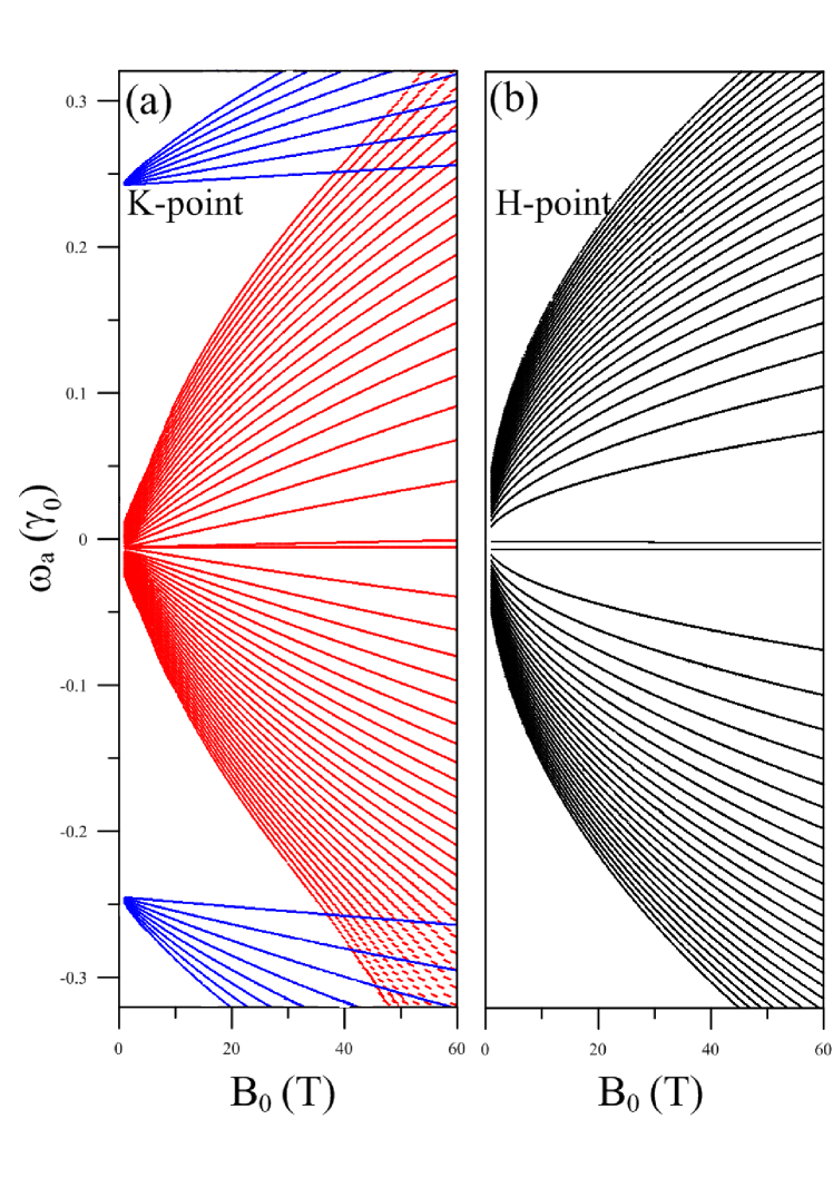
Figure 19: $B_{0}$-dependent energies of the (a) K-point and (b) H-point LSs.

The $k_{z}$-dispersed LSs are depicted from the zone boundary point K to H for $B_{0}=40$ T (Fig. 19 (a)). According to the zero-field band structure, the monolayer-like and bilayer-like signatures are deduced to coexist in Bernal bulk graphite. A series of subenvelope functions distributed among the four constituent sublattices are illustrated in Figs. 19 (b) and (c) for the Landau states at K and H points. The LSs can be classified into two groups (blue and red) according to the characteristics of the energy dispersions and the subenvelope functions. In the vicinity of the K point, the two groups are attributed to the magnetic quantization of the respective parabolic subband (blue and red in Fig. 15). In the 1st BZ, the onset LS energies are consistent with the cosine $E^{c,v}=2\gamma_{1}\cos(k_{z}I_{z})$ and flat $E^{c,v}=\sim 0$ dispersions along KH. As $k_{z}$ changes from K to H, the two groups merge to a series of double degenerate monolayer-like Landau states reflecting the zero interlayer atomic interactions. However, the splitting of the lowest $n^{c,v}=0$ LSs directly reflect the non-equivalent on-site energies of A and B sublatices. In general, away from the H point, the lift of degeneracy can be mainly attributed to the interlayer atomic interactions $\gamma_{1}$, $\gamma_{3}$ and $\gamma_{4}$.[92] The energy spacings of LSs are determined by the curvatures of the parabolic subbands. Near the K point, electron-hole asymmetry of LSs is presented under the influence of the interlayer atomic interactions, while it becomes symmetric for the monolayer-like LSs at the H point. Moreover, the K and H points correspond to band edges of LSs, where the Dirac quasi-particles are the dominant contributor in the magneto-optical properties. The effective mass model (only considering $\gamma_{0}$ and $\gamma_{1}$) can obtain qualitatively consistent calculations for the first few LSs. However, it misses the feature of the electron-hole asymmetry, which may be hardly observable in STS but has been validated to be significant in magneto-reflectence/absorption,[206, 82, 209] and magneto-Raman measurements.[207, 208]

At the K point, the first group of LSs appears at $E^{c,v}\simeq 0$, and the second group begin at $E^{c,v}\simeq 2\gamma_{1}$, where the subenvelope functions are associated in the way similar to the case of bilayer graphene. Accordingly, the numbers of the zero points of $B_{1}$ and $A_{1}$ are employed to define quantum numbers of the first- and second-group LSs, $n_{1}$ and $n_{2}$, respectively. That is, the relationship of the two groups is $A_{1}:A_{2}:B_{1}:B_{2}=n-1:n-2:n:n-1$ for $n_{1}=n\geq 2$ and $n:n-1:n+1:n$ for $n_{2}=n\geq 1$. As $k_{z}$ moves to H, with the increasing energy, the first group ascends while the second group descends according to the cosine dispersion $2\gamma_{1}\cos(k_{z}I_{z})$. Furthermore, the H-point subenvelope functions behave monolayer-like relationship, as depicted by the wave functions in Fig. 19 (c).

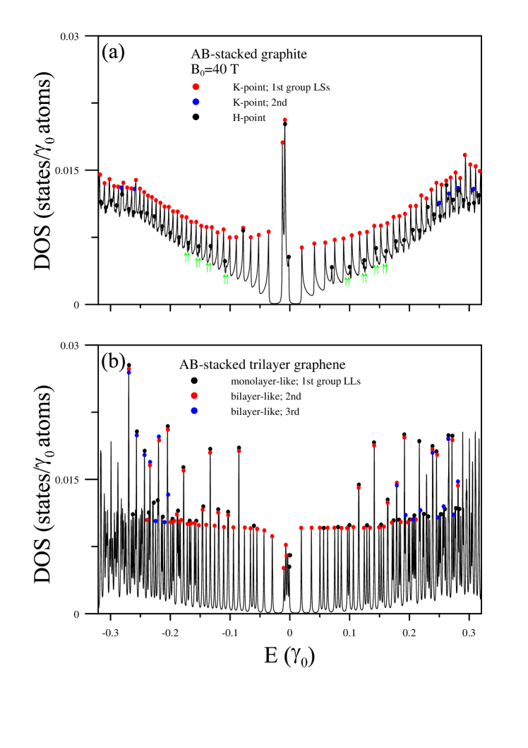
Figure 20: DOS of Bernal graphite at $B_{0}=40$ T. Also shown is that of Bernal trilayer graphene.

The profile of monolayer-like (bilayer-like) LSs in the H (K) point can be clearly seen from their energy evolution with the variation of the field strength, as shown in Fig. 20. Notably, the former is linearly dependent on $B_{0}$ and the latter exhibits a square-root $B_{0}$ dependence, as a consequence of massless and massive Dirac quasi-particles. It is shown in the K-point energy evolution that as compared to bilayer graphene, the energy spacings are significantly reduced and the onset energy of the second group of LSs is increased to twice the value of $\gamma_{1}$. This can be simply explained by the minimum model in which the in-plane dispersion at the K point is coupled with an vertical effective hopping energy of 2$\gamma_{1}$ between two neighboring layers. On the other hand, the monolayer-like energy evolution at H point comes from the fact that the state energies are correlated with only the nearest-neighbor in-plane hopping $\gamma_{0}$. However, the splitting of the lowest $n^{c,v}=0$ LSs is revealed only in the case of the non-equivalent on-site energies for A and B sublatices.

The DOS also reveals the prominent peaks with both the monolayer-like and bilayer-like signatures, which respectively originate from the vicinity of local extreme values of LSs at the H and K points, in Fig. 21 (a). This implies that the essential properties in Bernal graphite can be regarded as a combination of monolayer and bilayer graphenes, as well as display the linear and square-root dependence on $B_{0}$. In STS measurements,[74] the bilayer-like spectral features are relatively dominant and the valance DOS peaks are stronger than the conduction ones because the corresponding band curvature is relatively small. Furthermore, the energy dependences of the monolayer-like and bilayer-like LLs are also observed in the tunneling spectra of decoupled monolayer, bilayer and trilayer graphenes.[77] It should be noticed that the reduced peak spacings, Fermi velocity, effective mass and onset energy of the second group $2\gamma_{1}$ are important features to distinguish the bulk graphite from a bilayer graphene. While the graphene properties have been verified with STS in bulk graphites, there are still unsolved issuers for the tiny peaks resulting from the bulk properties of LSs between the K and H points.

4.3.2 Anticrossings of Landau subbands

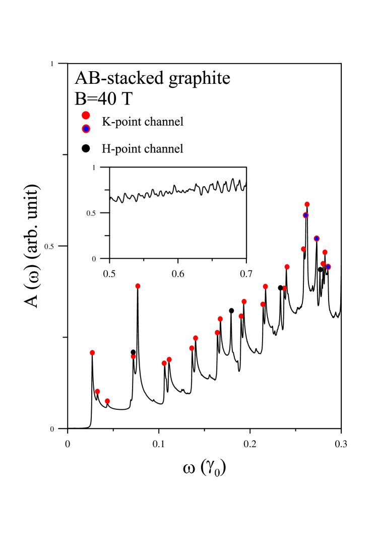
Figure 22: Magneto-absorption spectra of Bernal graphite. The absorption peaks corresponding to the transitions of massive (massless) Dirac fermions near the K (H) point are marked by red (black) dots.

The evolution of the LSs from K to H is responsible for the magnetic quantization for the transformation of the subbands from parabolic dispersion to linear dispersion, as shown in Fig. 22. As a result of the anticrossing of LSs, there are some tiny peaks appearing in couples between monolayer-like and bilayer-like LSs, as indicated by green arrows in Fig. 21(a). Such tiny peaks come from the band extrema of the reversed LSs around $k_{z}=0.8$, as shown in Fig. 22 (a). In the paper,[93] Nakao had explained the anticrossing phenomenon. They applied the perturbation method to calculate the lift of degeneracy and led to the conclusion that these level anticrossings are due to the trigonal warping effect of $\gamma_{3}$ in the LS spectrum. Also, the event is deduced to appear at the crossover of two LSs that satisfy the condition, $n_{1}-n_{2}=3I+1$, where I is an integer, that is; the two LSs have the same quantum mode for a certain kind of subenvelope function. The opening energy of the anticrossing LSs is more obvious in the stronger field. This phenomenon is also predicted in the LL spectra of AB- and ABC-stacked few-layer graphenes.[224, 31, 205] In addition, $\gamma_{2}$ and $\gamma_{5}$ also induce band edges for the first few valence subbands near the Fermi level.[92] These VHSs between K-H might be a cause for the unresolved DOS peaks in previous works.[75, 74]

In the anticrossing region, the mixture of the LLs caused by the trigonal parameter $\gamma_{3}$ can be realized by the evolution of the subenvelope functions of the LSs. The weight of the amplitude with respect to each sublattice has a significant hybridization alone $\widehat{k_{z}}$ for the $n^{c}_{1}=5$ LS that couples with $n^{c}_{2}=1$ LS, as shown in Figs. 22 (f)-(i). The behavior is distinct from the unhybridized LS, e.g., $n^{c}_{1}=2$ LS in Figs. 22 (b)-(e). For $n^{c}_{1}$=2 LS, as the state moves from K to H, its bilayer-like subenvelope functions gradually transform into monolayer-like ones, i.e., carrier distribution of two layers transfers into one of the two layers. The quantum mode of the dominating sublattice $B^{1}$ transforms from two to one. On the other hand, the evidence of the state hybridization of $n^{c}_{1}=5$ and $n^{c}_{2}=1$ LSs can be shown by the perturbed behavior of the subenvelope functions around the anticrossing center, $k_{z}\sim 0.8(\pi/2I_{z})$. A such state is a multi-mode state, composed of the main mode $n^{c}_{1}=5$ and the side mode $n^{c}_{2}=1$ LS, as depicted in the dashed rectangle. Nevertheless, at the H point, the wave function of the LS converts to the monolayer-like $n^{c}=1$ LS as a result of the vanished perturbation. It should be noted that the transition channels of the hybridized LSs might be too weak to observe in optical spectroscopy measurements, but might be observable in STS measurements.

4.4 Magneto-optical properties

Bernal graphite, with band profiles of monolayer and bilayer graphenes, is a critical bulk material for a detailed inspection of the massless and massive Dirac fermions. The recent surge in interest in 2D graphenes is based on the properties of bulk graphite. The monolayer-like and bilayer-like absorption spectra are predicted to coexist in the bulk spectrum as a result of the excitation channels between intragroup LSs near the H point and between two intragroup and intergroup LSs near the K point. Whether the optical transitions actually take place is subject to the relationship of the initial- and final-state subenvelope functions. According to $A(\omega)$, in Eqs. 38 and 39, it is deduced to that they must have the quantum-mode difference by one with regard to a same sublattice. The spectral profiles, such as peak intensity, frequency and numbers, can thus be described by the responses of the optical channels of the 1D LSs. Especially, near the band edges of the 1D LSs at the K and H points, charge carriers chiefly accumulate and predominate the optical excitations.

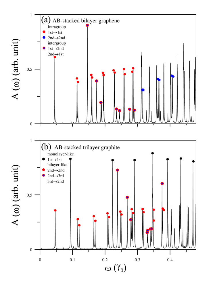
Figure 23: Magneto-absorption spectra of AB-stacked (a) bilayer and (b) trilayer graphenes.

The 1D-LS channels result in the square-root divergent peaks in the absorption spectra where two series of peaks, marked by red and black dots, correspond to the massive and massless Dirac fermions, respectively, as shown in Figs. 23. The K-point associated peaks can mainly be classified into four groups of peaks, resulting from two inter- and intra-group LS excitations. However, the intergroup ones are obscured due to the broadening peak width and relatively weak coupling of wavefunctions between the initial state and final state, especially for the region at higher frequencies. Except that the threshold peak comes from only one single channel, most of the K-point associated peaks come from pair channels, so called twin peaks. The splitting energy between the pair is induced by the electron-hole asymmetry; it decreases with increased frequencies or decreased field strengths. In contrast, owing to the subband symmetry at the H point, the degenerate channels give rise to only single-peak spectrum with relatively symmetric divergence form. All the such peaks can be precisely described by a monolayer graphene with only $\gamma_{0}$. Accordingly, the absorption spectrum of Bernal graphite displays both bilayer-like twin-peak structure and monolayer-like single-peak structure.

Spectral intensity is mainly determined by two factors: the $k_{z}$-dependent band-edge curvatures and the velocity matrix. It turns out that the H-point and K-point excitations have almost the same contribution to the magneto-absorption spectra, in spite of two times more excitation numbers for the former, according to the DOS shown in Fig. 2-4. The optical transition rate depends on the expectation value of the velocity matrix, which can be divided into several components of wavefunction products each with their own respective integral hoppings $\gamma^{\prime}$s. However, because $\gamma_{0}$ is at least one order larger than the others, the optical transition rate is simplified as an inner product of the same-layer A and B subenvelope functions of the initial and final states. Based on the $k_{z}$-evolution of the subenvelope functions described in Chapter 4.3.1, the strong-strong combination at H is a evidence of the comparable intensity of the Dirac quasi-particles in the H- and K-related spectra.

There are some inconspicuous absorption peaks that come from the band-edge states of the anticrossing LSs, which satisfy the selection rules of modulo 3, instead of the principle selection rule that characterizes the prominent K-point and H-point peaks, in Fig. 23. One can ascribes the specific selection rules to the hybridization of the anticrossing LSs, which is determined by interlayer atomic interactions $\gamma_{3}$ (Chapter 4.3.2). Therefore, the inconspicuous peaks have relatively weak intensities than the K-point and H-point peaks, not only because of the smaller DOS but also because of the smaller velocity matrix. These extra peaks are also studied in graphene systems,[128, 228] especially for the severely symmetry breaking structures, such as AAB-[25] and sliding bilayer graphenes.[35] This indicates that obtaining a comprehensive description of graphene and graphite systems requires the full atomic interactions of SWM model for its accurate calculations of the velocity matrix and characterization of the wave functions.

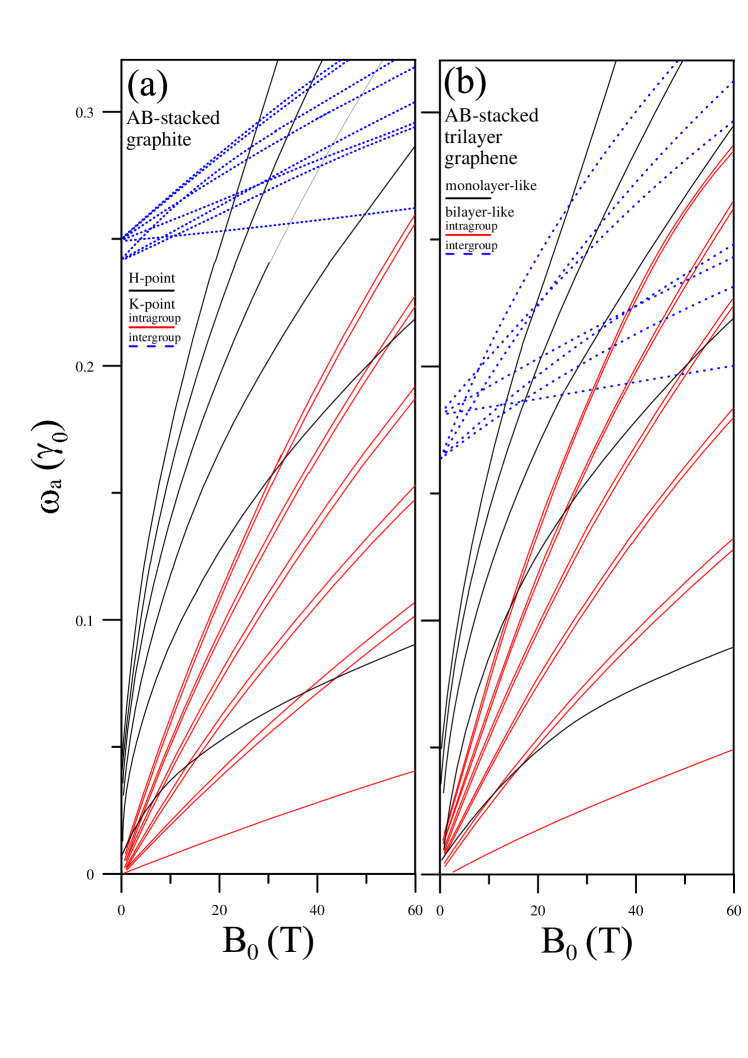
Figure 24: $B_{0}$-dependent absorption frequencies of Bernal (a) graphite and (b) bilayer and trilayer graphenes.

In graphenes, the spectral peaks are shaper and more distinguishable than those in graphite due to the stronger Landau quantization effect in 2D materials, as shown in Fig. 24. The excitation channels in bilayer graphene resemble the K-related ones in Bernal graphite, while the absorption peaks are delta-function-like, reflecting the 0D dispersionless LLs as in the 2D systems. This is in contrast to the square-root-like divergent form of the absorption peaks in 3D bulk systems as a result of the 1D dispersive LSs along out-of plane direction. Also, the absorption spectrum presents twin-peak structures due to the splitting of dual channels, with an smaller splitting energy of $\sim$10 meV and half-reduced onset energy $\gamma_{1}$, as compared to the Bernal graphite. In the case of trilayer AB-stacked graphene, the magneto-absorption spectrum is regarded as a combination of a monolayer-like and a bilayer-like spectra. The former exhibits a predominantly uniform intensity with single-peak structures similar to the H-point characteristics in graphite. However, the latter displays half-intensity twin peaks corresponding to the splitting of the dual channels in the electron-hole asymmetric LL spectrum. In addition, the absence of intergroup excitations between bilayer-like and monolayer-like LSs is due to the anti-symmetric phase relation in the velocity matrix.

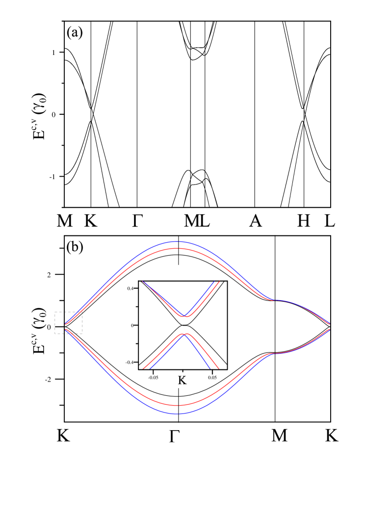
Figure 25: Band structure of rhombohedral (a) graphite and (b) trilayer graphene.

The optical channels at K and H points show two kinds of field evolutions of the absorption frequencies, as shown in Fig. 25. The former type behaves as a linear dependence of $B_{0}$ whereas the latter is square-root like, as depicted by the black and red solid curves in Fig. 25(a). The absorption frequencies related to H point are identical to those of monolayer graphene and can well described by a $\sqrt{nB_{0}}$ relationship. (Fig. 14(a)). However, compared to the bilayer spectrum (Fig. 25(b)), the splitting in double peaks is a bit enhanced for the K-point channels because of the amplification of interlayer atomic interactions in graphite. In short, both AB-stacked graphene and graphite exhibit massless and massive Dirac-fermion properties in the optical absorption spectra with or without magnetic fields. The induced spectral features, such as the frequency dependence, peak width, divergent form and onset energy $\gamma_{1}$, are the signatures that can be used to distinguish between Bernal graphite and graphene. It should be noticed that the twin peaks are sensitive to the magnetic field strength. However, the observability in optical spectroscopy depends on how the magnetic field compete with the experiment resolution and ambient temperature. These main features are very useful information in identifying the stacking configurations and dimensionality of systems from experimental measurements.

Magneto-optical spectroscopy provides useful insight into the LSs in graphite materials. The optical response of the Dirac quasi-particles is a dominant contributor in the magneto-optical properties. Infrared magneto-transmission studies mainly focus on detailed information about the differences between graphites and multilayer epitaxial graphenes.[86, 82, 83, 200, 209, 84, 85, 210] Reflect the bilayer-like parabolic dispersion, A series of absorption peaks of energy scaled as linear-$B_{0}$ is present in the spectra and identified as contributions from massive Dirac fermions in the vicinity of the K point.[86] By fitting the linear relationship and selection rule $\Delta n=\pm 1$, the effective interlayer interaction $2\gamma_{1}$ at the K point is obtained in the framework of the minimal model. The deduced value is actually about double of that in bilayer graphene. However, reflecting the inherent complexity of the SWM model, there is an evidence of the splittings of channels at the K point, attributed to electron-hole asymmetry. This is also observed in magneto reflection[206], magneto-absorption[82, 209] and magneto-Raman experiments.[207, 208] The experimental results indicate that the full SWM model including additional interlayer atomic interactions well describes the electron-hole LS asymmetry.

The monolayer-like spectra are verified by a series of inter-LS transitions with a characteristic magnetic field frequency dependence $\omega\propto\sqrt{nB_{0}}$ at the H point.[209, 84, 200, 85, 86] The measured dependence can be used to directly obtained the value of $\gamma_{0}$ in graphite. The full SWM model provide a basic interpretation in such a case to clarify the optical response of the graphene layers and get a quantitative agreement between optical experiments and theory. However, there is also an evidence of splitting of the degenerate channels the H point.[209, 84, 200, 85] It is confirmed that the observed splitting is not associated to the electron-hole asymmetry of the Dirac cone. The splitting of the degenerate channels might be attributed to the on-site energy difference between A and B sublattices, spin-orbital coupling, anticrossing of LSs or parallel magnetic flux. Nevertheless, these results require a more elaborated model and clearer experimental evidences. While the trigonal warping affects the anticrossings of the LSs in the low-energy region, a new series of absorption peaks obeying new selection rules might possibly be observed with the increased hybridization of the coupled LSs.

Magneto-optical spectroscopies have also been used to study the massless and massive Dirac fermions in 2D AB-stacked few-layer graphenes. The electron-hole asymmetry is also reported on bilayer graphene with cyclotron resonance[211], ARPES[177] and infrared spectroscopy,[9, 213] which is mainly under the influence of $\gamma_{2}$ and the in-equivalent environments of the two sublattices. The infrared transmission spectrum of ultrathin graphene (3-5 layers) indicates that two series of $B_{0}$- and $\sqrt{B_{0}}$-dependent frequencies are observed for the low-lying inter-LL excitations of the massless and massive quasiparticles, respectively.[215] Magneto-Raman spectroscopy has also been used to probe the those Dirac-like optical excitations in few-layer graphenes.[217, 216] However, further experiments of the higher excitation channels is needed for identifying the other energy deoendence of the higher LLs away from the Fermi level. The optical experiments can be used to determine the interlayer atomic interactions that dominate the electron-hole asymmetry and LL and LS dispersions. The linear and square-root energy relationships of Dirac-like magneto-channels can be found in few-layer graphenes and graphite, while the differences between the interpreted values of $\gamma$’s can distinguish the stacking layer, configuration and dimensionality.

5 Rhombohedral graphite

5.1 Electronic structures without external fields

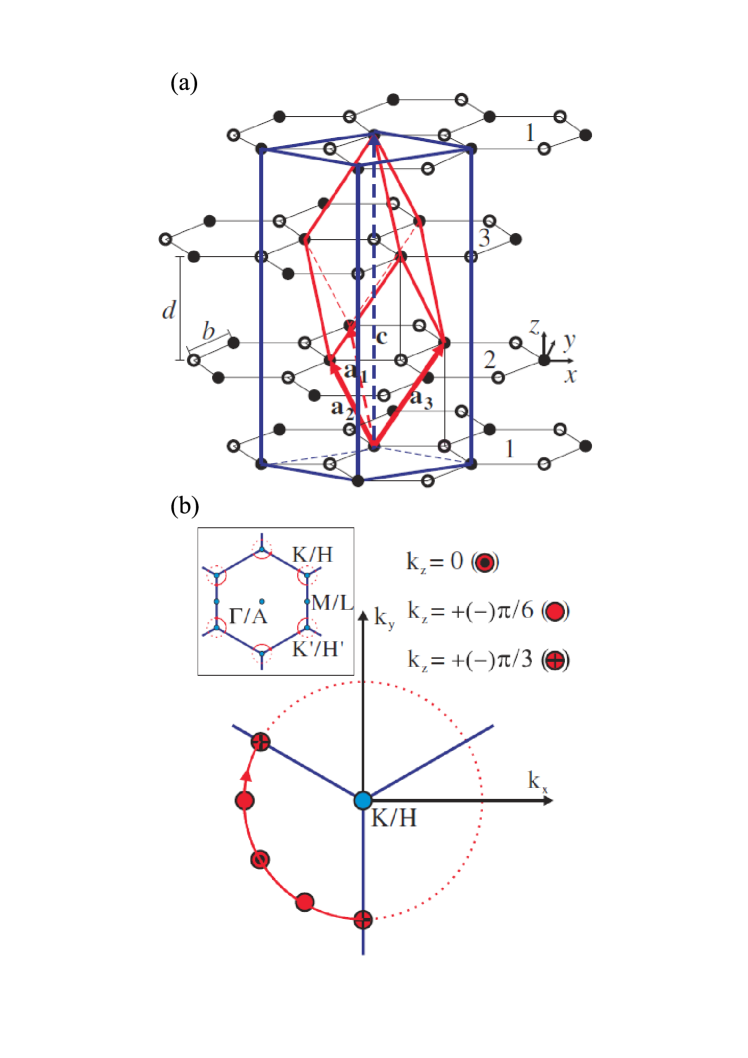
Figure 26: (a) Rhombohedral primitive unit cell (red color) and triple hexagonal unit cell (blue color). (b) ($k_{x},k_{y}$)-projection of the Dirac-point spiral at $k_{z}=0$, $k_{z}=\pm\pi/6$ and $k_{z}=\pm\pi/3$.

In the hexagonal unit cell with $p_{3}$ symmetry,[220] the energy dispersions of the rhombohedral graphite are depicted along different symmetric directions, as shown in Figure 26. The band structure consisting of three pairs of occupied valence and unoccupied conduction subbands is highly anisotropic and asymmetric about the Fermi level. The in-plane energy bands show linear or parabolic dispersions, whereas they weakly depend on $k_{z}$. For the KM$\Gamma$K plane at $k_{z}=0$, the K, M, and $\Gamma$ points are the local maximum (minimum), saddle, and the maximum points, respectively. They would induce large DOS and greatly affect optical excitations. Near the K point, the first pair of subbands, crossing across the Fermi level, exhibit linear dispersion without degeneracy. The second pair are double-degenerate parabolic subbands; however, the broken degeneracy along $\Gamma$K leads to three non-degenerate parabolic subbands at middle energies $\sim\pm 2B_{0}$. When the plane is shifted from $k_{z}=0$ to $k_{z}=\pi/3I_{z}$, similar in-plane dispersions are also revealed in the HLAH plane. However, the pair of linear bands is located at the HA line instead of the HL line. In particular, the energy subband along KH becomes a three-fold degeneracy with a very weak $k_{z}$-dependent dispersion (inset in Fig. 26). Moreover, small free-carrier pockets are formed near K-H region, because the intersection of valence and conduction linear subbands crosses $E_{F}=0.007$ with a very weak dispersion.

Remarkably, one pair of linear subbands always show up at the $(k_{x},k_{y})$ plane, regardless of the value of $k_{z}$. This means that the existence of Dirac cones in Rhombohedral graphite with the Dirac points spirally distributing with $k_{z}$ about the high symmetry line along K-H. Besides, the parabolic subbands are attributed to zone folding,[124] because the Hamiltonian (Eqs. (22)-(24)) is built in the triple hexagonal unit cell instead of in the primitive unit cell, which is a rhombohedron with space group symmetry $R\overline{3}m$.

In the next section, a analytic solution for the 3D Dirac cones is calculated in the primitive unit cell along the highly symmetric points by using the effective-mass model with only $\gamma_{0}$ and $\gamma_{1}$.[221, 125, 222] The trajectory of the Dirac-cone movement is a function of $k_{z}$. Furthermore, the distortion and anisotopy of the Dirac structures have also been studied separately under the influence of the other interlayer atomic interactions.[124]

5.2 Anisotropic Dirac cone along a nodal spiral

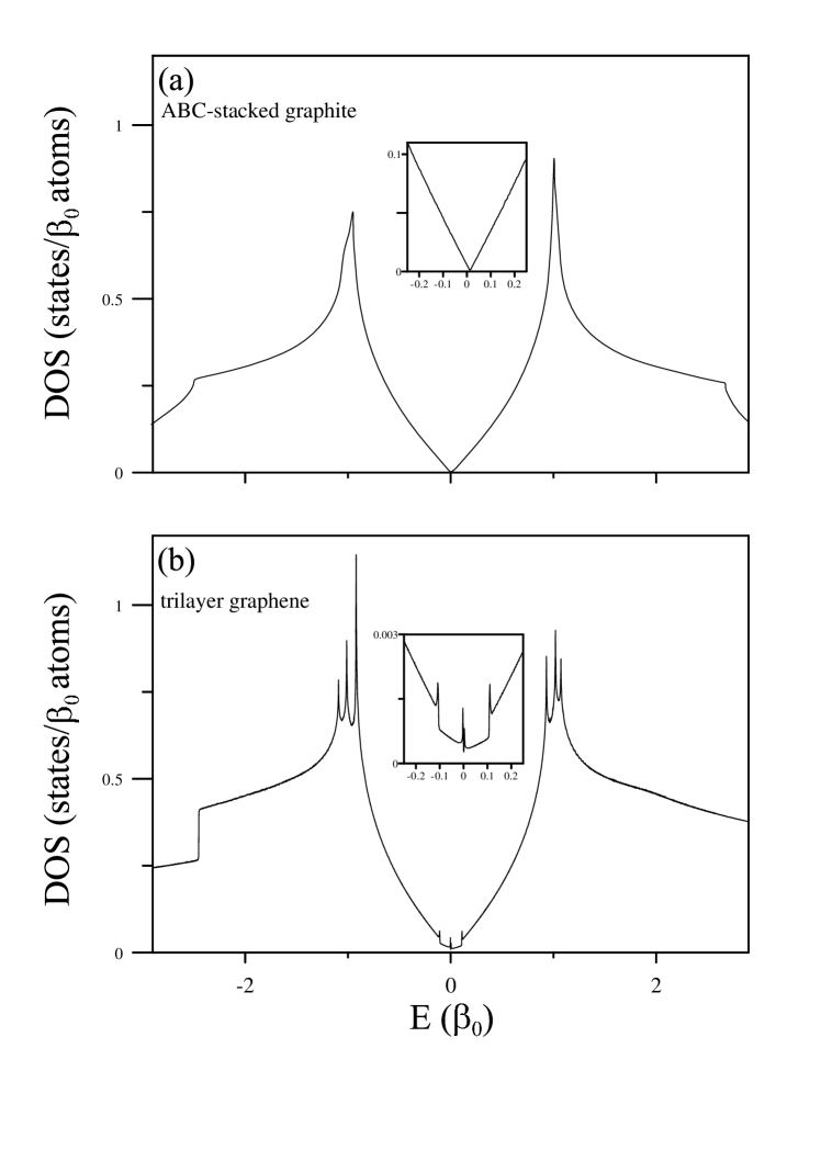
Figure 27: DOSs of ABC-stacked (a) graphite and (b) trilayer graphene.

The primitive unit cell of a rhombohedral graphite is defined in Fig. 27 (a), which is 1/3 of the volume of the hexagonal unit cell in Fig. 26. The three primitive unit vectors $a_{1}$, $a_{2}$, and $a_{3}$ are related to the c-axis: 3$I_{z}\widehat{\mathbf{z}}=\sum_{i=1}^{3}\mathbf{a}_{i}$, where $a_{1}=a_{2}=a_{3}$, and the angles between two primitive vectors are the same. A rhombohedron with six identical faces is referred to as the primitive cell in ABC-stacked graphite. The Dirac-type dispersion is obtained under a continuum approximation for the low-energy band structure in the vicinity of the H VK VH hexagonal edges specified in Fig. 27 (b). With the the BZ edge served as a reference line, the energy dispersion is described as a function of the 3D wave-vector measured from the BZ edges.

Based on the two sublattices, a full tight-binding Hamiltonian is represented by a $2\times 2$ matrix

$$H_{ABC}=\left\{\begin{array}[]{cc}H_{1}&H_{2}\\ H_{2}^{\ast}&H_{1}\\ \end{array}\right\}\text{,}$$ (47)

where $H_{1}$ and $H_{2}$ take the form

$$\begin{array}[]{l}H_{1}=2v_{4}\hbar k\cos(\phi+k_{z})+2v_{5}\hbar k\cos(\phi-2k_{z})\text{,}\\ H_{2}=-v_{0}\hbar k\exp(-i\phi)+\beta_{1}\exp(-ik_{z})+\beta_{2}\exp(-i2k_{z})\\ +v_{3}\hbar k\exp[i(\phi-k_{z})]+v_{5}^{\prime}\hbar k\exp[i(\phi+2k_{z})\text{.}\end{array}$$ (51)

The perpendicular wave-vector components $k_{z}$ is scaled by $1/d$ and the variables $k$, $\phi$ and $v_{m}^{\prime}$ are defined as follows: $k=\sqrt{k_{x}^{2}+k_{y}^{2}}$, $\phi=\arctan(k_{y}/k_{x}-7\pi/6)$ and $v^{(\prime)}_{m}=3b|\beta^{(\prime)}_{m}|/2\hbar(m=0,3,4,5)$. This chiral Hamiltonian characterizes the inversion symmetry, and its eigenvalues are calculated as

$$E=H_{1}\pm|H_{2}|\text{.}$$ (52)

In Eq. (45), the off-diagonal elements can be written as $H_{2}=f(k_{x},k_{y},k_{z})+\beta_{1}\exp(ikz)$, where $|f|\simeq[v_{0}^{2}+v_{3}^{2}-2v_{0}v_{3}\cos(2\phi-k_{z})]^{1/2}\hbar k$ as $\beta_{2}$ and $\beta_{5}^{\prime}$ are neglected. This indicates the same chirality in rhombohedral graphite and in, while $\beta_{1}$ induces an offset energy from the hexagonal edge for the Dirac point. On the other hand, the identical diagonal elements lead to gapless Dirac cones, and their linearity in $k$ implies the possibility of cone tilting. Moreover, the zone-folded parabolic bands are absent in the primitive rhombohedral representation.

By ignoring $\beta_{2}$, $v_{4}^{\prime}$ and $v_{5}$, the coordinate $(k_{D},\phi_{D})$ and the energy $E_{D}$ of the Dirac point are, respectively, expressed as follows in the case of $H_{2}=0$:

$$k_{D}=\beta_{1}(v_{0}\hbar)^{-1}[1+(v_{3}/v_{0})\cos(3k_{z})]$$ (53)

$$\phi_{D}=-k_{z}+(v_{3}/v_{0})\sin(3k_{z})\text{,}$$ (54)

and

$$E_{D}(k_{D}(k_{z}),\phi_{D}(k_{z}))=2\beta_{1}(v_{5}/v_{0}+v_{3}v_{4}/v_{0}^{2})\cos(3k_{z})\text{,}$$ (55)

up to first-order perturbation $\mathcal{O}(v_{3}/v_{0})$. In particular, the Dirac point displays a spiral dispersion as a function of $k_{z}$. In terms of polar coordinates $(q,\theta)$ and the coordinate transformation $q^{2}=k^{2}+k_{D}^{2}-2k_{D}k\cos(\phi-\phi_{D})$, the Dirac-type energy dispersion in Eq. (47) can be simply expressed as

$$E(q,\theta,k_{z})=E_{D}\pm\epsilon(q,\theta,k_{z})\text{,}$$ (56)

where

$$\epsilon(q,\theta,k_{z})=[v_{0}-v_{3}\cos(2\theta-k_{z})\pm 2v_{4}\cos(\theta+k_{z})]\hbar q$$ (57)

describes the dispersion of the anisotropic Dirac cone, and the + and - signs refer to the upper and lower half Dirac cones, respectively. By the minimal model with only $\beta_{0}$ and $\beta_{1}$, the Dirac cone is identical to that of monolayer graphene with a Fermi velocity $v_{0}$.[125] The spiral of the Dirac point is described as a function of $v_{0}$ in the case of $v_{3}=v_{4}=0$, which lies on a cylindrical surface of radius $\beta_{1}(v_{0}\hbar)^{-1}$ with the spiral angle $\phi_{D}$ in sync with $-k_{z}$. However, taking into account the interlayer hoppings $v_{3}$ and $v_{4}$, we find that the spiral becomes non-cylindrical and exhibits $k_{z}$-dependent anisotropy. The former and the latter, respectively, keeps and reverses the sign under a phase shift $\theta\rightarrow\theta+\pi$; they, respectively, cause a rotation and tilt of the Dirac cones as a function of $k_{z}$. The previous works[124] have demonstrated the anisotropic tilt of the Dirac cones that vary in orientation and shape with $k_{z}$ along the Dirac-point spiral. The Dirac-point spiral across $E_{F}$ indicates the semimetallic properties, while the band overlap $\simeq 10$ meV according to Eq. (50) is one (two) order of magnitude smaller than that in Bernal graphite (simple hexagonal) graphite. Near $k_{z}=0(\pm\pi/3)$, there is an electron (hole) pocket, and at $k_{z}=\pm\pi/6$, the free-carrier pockets shrink to the Dirac point, i.e, the location of the Fermi level $E_{F}=E_{D}(\pi/6)=0$. This phenomenon is also demonstrated in the hexagonal unit cell (Fig. 26). Similar analysis can be performed for the H-K-H edge extension, around which the spiral angle synchronizes with $k_{z}$ and the chirality is reversed.

5.3 dimensional crossover

The 3D characters of the electronic properties are significant for the dimensional crossover from the 2D few-layer graphene to the 3D bulk graphite.[223] ABC-stacked configuration gives rise to different lattice symmetries for the 2D and 3D systems. With the periodic stacking of graphene sheets, the bulk graphite has a biparticle lattice symmetry belonging to the space group $R\overline{3}m$. Its primitive unit cell is a rhombohedron containing two atoms, designated as A and B in Fig. 27 (a). In contrast, the N-layer ABC-stacked graphene has two atoms on each layer, i.e., total of 2$N$ atoms. Therefore, it is clear to figure out the distinction of the energy bands between both systems. The low-energy electronic properties in the bulk graphite is described by the 3D anisotropic Dirac cones tilted relative to $\widehat{k_{z}}$. On the other hand, the few-layer case is characterized by one pair of partially flat subbands at $E_{F}=0$, which is mainly contributed by the surface-localized states.[224, 225] Such appearances of subbands, irrelevant to the bulk subbands, indicate the dimensional crossover from graphite to few-layer graphene.[223] Nevertheless, the weakly $k_{z}$-dependent dispersion across $E_{F}=0$ displays a semi-metallic behavior for the bulk graphite, making it a candidate system for the observation of 3D QHE.[122, 125] Besides, there are sombrero-shaped subbands near $\beta_{1}$, which can be used as an interpretation of the dimensional crossover of the 3D case to the 2D limit.

The DOS is very useful for understanding the optical properties. Its main characteristics are responsible for the Dirac cones that spiral down as $k_{z}$ varies. In the low-energy region, the DOS intensity increases nonlinearly with the increasing $\omega$, as shown in Fig. 28 (a). At $\omega=0$, a sharp valley is formed due to the fluctuation of Dirac-point energies within $E_{F}-$5 meV $\thicksim E_{F}-$5 meV. Furthermore, a cave structure consisting of a local maximum and a local minimum is formed near $\omega\simeq$ (-) 0.09 $\beta_{0}$ for conduction (valence) DOS.[220] The nonlinear dependence of $D(\omega)$ is attributed to the deformation of the isoenergy surface of the anisotropic Dirac cones, as indicated by the insert of Fig. 28 (a). However, when $\omega$ exceeds the nonmonotonous structure, $D(\omega)$ becomes linearly dependent on $\omega$ as a consequence of the restoration of Dirac cones. In the middle-energy region, the smoothly enhanced DOS is contributed by the parabolic subbands, while the prominent peak near $E^{c,v}\simeq\pm\beta_{0}$ is a bit broader than that of monolayer graphene as a combination of a series of in-plane saddle-point states in the 3D $\mathbf{k}$ space.

For ABC-stacked graphene, the dimensional crossover of electronic properties is revealed by 2D divergent structures in the DOS.[226] The DOS is nearly symmetric about the Fermi level, as shown in Fig. 28 (b). At low energies, an evidence for the partial flat bands near the $E_{F}$ is revealed by a symmetric broadening peak in the STS measurements.[118, 117] Those away from $E_{F}$ originate from the sombrero-shaped and parabolic subbands. Consequently, the low-energy features in ABC-stacked graphenes are dominated by the surface-localized states. Beside, the saddle-point states at middle energies induce three symmetric peaks. These are contrast to the valley and cusp DOS in the 3D bulk $\mathbf{k}$ space. The differences between ABC-stacked graphenes and graphites are mainly caused by the different stacking symmetries and the reduction of dimension, which would be reflected in the absorption spectra $A(\omega)$.

5.4 Optical properties without external fields

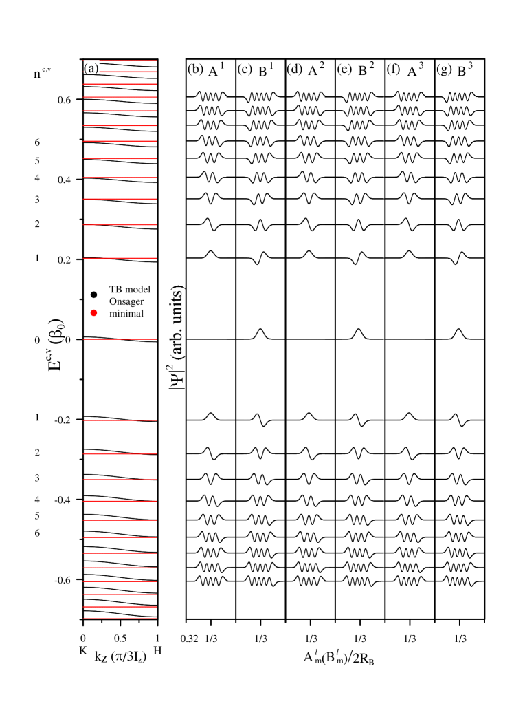
Figure 29: (a) The $k_{z}$-dependent Landau subbands at $B_{0}=40$ T. The black and blue colors, respectively, represent the calculations from the full tight-binding model and the minimal model. (b)-(g) The subenvelope functions at the K point.

Absorption spectrum of rhombohedral graphite reflects the Dirac-cone energy dispersions, as shown in Fig. 29 (a). In general, the low-frequency intensity increases approximately linearly with the increasing $\omega$, as a result of the excitations within the Dirac cones that spiral around K (K^′) corner, where the Dirac points are fluctuated within a narrow range $E_{F}-5$ meV $\thicksim E_{F}$+5 meV.[227] However, the interlayer atomic interactions distort the Dirac cones and slightly break the linear dependence of the absorption intensity on the frequency.[220] The small valley at $\sim 0.2$ $\beta_{0}$ is associated with the transition between the caves in the DOS (Fig. 28 (a)). As the energy dispersion transforms from linear to parabolic ($\omega\gtrsim 1.0$ $\beta_{0}$), the spectra deviate from the linear dependence. In the middle-energy region, the enhanced $k_{z}$ dependence of the parabolic subbands induces a wider distribution of the spectral structure. There are two separated peaks at $\omega\sim 1.95$ $\beta_{0}$ and $\omega\sim 2.0$ $\beta_{0}$ (blue circles); they solely come from the excitations from the BZ edges M and L, respectively. The second peak is higher than the first one because of the higher JDOS and transition probability.

In a N-layer ABC-stacked graphene, the optical absorption spectrum is richer than that of graphite in both the low- and middle-frequency regions, as a result of the more N$\times$N kinds of excitation channels.[228, 229] For example of the trilayer case, the vertical transitions near the K point among different low-lying subbands give rise to feature-rich structures at low energies, including asymmetric peaks and shoulders, as shown in Fig. 29 (b). The middle-frequency channels also lead to several obvious peaks associated with the saddle-point states near the M point. It should be noted that the threshold peak, due to the vertical transitions between the surface-localized and sombrero-shaped subbands, is prominent at $\omega\sim\beta_{1}$ as a dominance of the surface-localized states in the DOS. Optical transmission spectroscopy has been used to verify the optical excitations related to the surface-localized and sombrero-shaped subbands.[229, 230]. These experimental evidences identify the dimensional crossover from ABC-stacked 3D graphite to 2D graphene.

5.5 Magneto-electronic properties

5.5.1 Tight-binding model

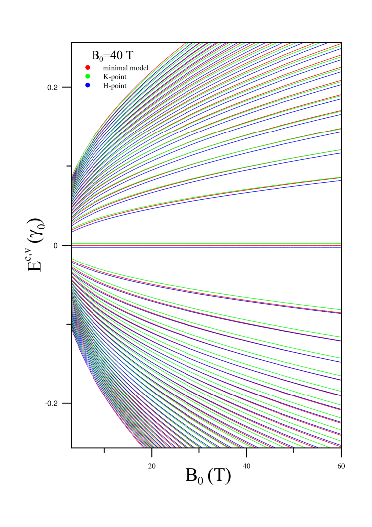
Figure 30: $B_{0}$-dependent Landau subband energies of rhombohedral graphite.

The LS spectra in rhombohedral graphite are calculated by a diagonalization scheme designed for the Peierls tight-binding Hamiltonian in the representation of the triple hexagonal unit cell.[231] The main characteristics of the spectra exhibit a definitely discernible 3D semi-metallic behavior, as compared to that of Bernal graphite and simple hexagonal graphite (small by one or two orders of magnitude), as shown in Fig. 30(a) for $B_{0}=40$ T. Due to the triple-size enlarged unit cell, the degeneracy of LSs is deduced to be $3\times 4$ for a single LS at a specific $k_{z}$ point in the hexagonal 1st BZ. With the ABC-sacking sequence, its bulk limit has the specific group symmetry $R\overline{3}m$, containing two atoms in a primitive unit cell in comparison to 2N atoms for a N-layer 2D case. This results in very distinct magneto-electronic properties between both systems. Accordingly, the LSs (LLs) for the cases of bulk graphite and the N-layer graphene are, respectively, classified as one-group and N-group[224, 31, 231].

The energy dispersions of LSs actually display a $k_{z}$ dependence consistent with the behavior of the zero-field band structure, in which the Dirac-point spiral dispersion in Eq. (50) corresponds to the $n^{c,v}=0$ LSs. The behavior of the subenvelope functions provides an evidence that also suggests the magnetic quantization of Dirac cones.[232] Their relationship between A and B sublattices is independent on $k_{z}$, and the same as that obtained from a comparative diagonalization for monolayer graphene ( e.g., at $k_{z}=\pi/6$ $I_{z}$ in Figs. 30 (b)-(g)). The subenvelope function of the $n^{c,v}$ LS consists of quantum modes $n^{c,v}$ and $n^{c,v}-1$ on sublattices B and A, respectively, where $n^{c,v}-1>0$. In particular, the $n^{c,v}=0$ LSs are characterized by the same pseudo spin polarizations on A sublattice. The reversed pseudo spin polarization on B is held by part of degenerate states. Within the first-order minimal model, the Dirac-point spirals can be topologically stable by the chiral symmetry, meaning that the interlayer atomic interactions are not obvious in the diagonalization results.[233]

Remarkably, in the minimal model, as a consequence of the magnetic quantization on the Dirac cones, the LS spectrum is dispersionless as function of $k_{z}$, as shown by the red curve in Fig. 30 (c). However, the effect of full interlayer interactions reflects the dimensional crossover for the Dirac cone and LS spectra in the rhombohedral graphite. While the properties of Dirac cones are preserved during the variation of $B_{0}$, these discernible 3D characteristics, deviated from $\sqrt{n^{c,v}B_{0}}$ dependence, are presented by $\beta_{3}$ and $\beta_{4}$ in terms of the tilt and distortion of the Dirac cones. In the next section, Onsager quantization method is used to give analytic energy solutions, and leads to the identification of the effects of the critical atomic interactions on the LSs along a nodal spiral.

5.5.2 Onsager quantization

The Onsager quantization rule is used to obtain the quantized energies for the Landau states of an isoenergetic surface along the Dirac point spiral.[124] According to the energy dispersion in Eq. (51), the area $S(\epsilon,k_{z})$ enclosed by the contour of energy $\epsilon$ is calculated from

$$S(\epsilon,k_{z})=\int_{0}^{2\pi}d\theta\int_{0}^{Q(\epsilon)}\epsilon(q,\theta,k_{z})q\cdot dq\text{.}$$ (58)

Using Eq. (51) and trigonometric substitutions, the integration is approximated as

$$S(\epsilon,k_{z})\simeq\pi\epsilon^{2}/v_{0}^{2}\hbar^{2}[1-(v_{3}/v_{0})^{2}]^{-3/2}\{1+6(v_{4}/v_{0})^{2}[1+2(v_{3}/v_{0})\cos(3k_{z})]\}\text{.}$$ (59)

The Onsager quantization condition is given by

$$S(\epsilon,k_{z})=2\pi eB_{0}\hbar n^{c,v}\text{,}$$ (60)

where the zero phase shift results from the same electron chirality and Berry phase as in monolayer graphene, regardless of the anisotropy of the Dirac cones. By neglecting interlayer atomic interactions, the quantized Landau energies are obtained for an isolated Dirac cone. i.e.,

$$E^{(0)c,v}(n^{c,v})=\pm\hbar v_{0}\sqrt{2eB_{0}n^{c,v}/\hbar}\text{,}$$ (61)

which turns into

$$E^{(0)c,v}(n^{c,v})F(k_{z})$$ (62)

for the tilted Dirac cone in rhombohedral graphite, where $F(k_{z})=[1-(v_{3}/v_{0})^{2}]^{3/4}\times\{1-3(v_{4}/v_{0})^{2}[1+2(v_{3}/v_{0})\cos(3k_{z})]\}$ is used to describe the dispersion factor as a consequence of the variation of the enclosed area. The energies of LSs is then obtained by superimposing the dispersions, Eq. (57), on the Dirac point $E_{D}$, Eq. (50), i.e.,

$$E^{c,v}(n^{c,v},k_{z})=E_{D}+E^{(0)c,v}(n^{c,v})F(k_{z})$$ (63)

According to the lowest LS in Eq. (58), $E^{c,v}(n^{c,v}=0,k_{z})=E_{D}\propto\cos(3k_{z})$, the Fermi level is determined at the point $k_{z}=\pi/6$, as the field strength allows the formation of LS bulk gaps, i. e., $B_{0}\geq[E_{D}(k_{z}=0)-E_{D}(k_{z}=\pi/3)]^{2}/v_{0}^{2}e\hbar\simeq 0.11$ T. Therefore, the renormalized Fermi velocity is given by

$$v_{F}(k_{z}=\pi/6)=v_{0}[1-(v_{3}/v_{0})^{2}]^{3/4}[1-3(v_{4}/v_{0})^{2}]^{1/2}.$$ (64)

At $B_{0}=40$ T, the energy dispersions of LSs are plotted from $k_{z}=0\sim k_{z}=\pi/3I_{z}$, as shown in Fig. 30. Also plotted are the calculations from the numerical diagonalization and the minimal model. In the minimal model, the LS dispersion and the Fermi velocity are obtained by keeping only $v_{0}$ and $v_{1}$ in Eqs. (58) and (59). The calculated LSs are dispersionless in the 3D momentum space and the Fermi velocity is $v_{F}=v_{0}$, as a result of the identical isotropic Dirac cones along a dispersionless Dirac-point spiral. However, the full tight-binding model brings about characteristics beyond the minimal model. Within a Dirac cone, the quantized Landau energies are symmetric about its Dirac point, based on Eq. (56), while the spiral localization of the Dirac points gives rise to the electron-hole asymmetry, as shown in Figs. 3-4 (a) and (b). This is interpreted as a consequence of due to $v_{3}$ and $v_{4}$, causing a narrow excitation energy range for a single channel, $n^{v}\rightarrow n^{c}$, which might be observed in optical experiments. Low-lying LSs are weakly dispersive in contrast to both AA- and AB-stacked graphites. In particular, only the $n^{c,v}=0$ LS moves across the Fermi level. The LS spacings are also reduced due to the renormalization of the Fermi velocity. Moreover, the bulk gap can be closed for higher LSs ($n^{c,v}\gtrsim 25$), because of the enhanced $k_{z}$ dispersion. The LSs calculated from Onsager quantization are consistent with those from the numerical diagonalization for $n=0,1,2,3,4$. The agreement of the magnitude holds up to $n^{c,v}=18\simeq\pm 730$ meV. However, the inconsistency coming from the continuum approximation is more apparent for higher $n^{c,v}$.

The magnetically quantized DOS of rhombohedral graphite is plotted in Fig. 32 (a). In the framework of the minimal model, the DOS peaks of rhombohedral graphite are identically reduced to 2D delta-function-like peaks of monolayer graphene, because the Dirac cones are isotropic and circularly distributed at $E_{F}=0$. In particular, all the peaks are equal-intensity and symmetric about the Dirac points at $E_{F}=0$. Under the influence of $\beta_{3}$ and $\beta_{4}$, the isotropic Dirac cones become tilted, anisotropic and spiral near the edge of BZ. The equal-intensity peaks transform into nonequal-intensity double peaks whose widths are determined by the $k_{z}$ dispersions of the 1D LSs. Each peak has two square-root divergent forms corresponding to the band-edge energies at the K and H points, (green and blue dots). Dirac-point spiral causes the particle-hole asymmetry, which furthermore destroys the anti-symmetric dispersions of LSs in the BZ, leading to different DOS intensities for valence and conduction LSs.

On the contrary, the DOS of ABC-stacked trilayer graphene exhibits three groups of symmetric delta-function-like peaks, which are not regularly sequenced according to the dispersionless LLs of three different subbans, as shown in Fig. 32 (b). Different characteristics of the three groups of LLs are clearly shown. The first peak at the Fermi level is composed of three surface-localized LLs; therefore, its intensity is approximately estimated to be three times than other peaks. Furthermore, peaks are densely formed for $\omega\gtrsim\beta_{1}$, which approaches to the crossover of the onset energies for the second and third groups. While the low-lying peaks in ABC-stacked fewlayer graphenes have been confirmed by STS, the essential differences between ABC-stacked graphites and graphenes need to be further verified.

5.6 Magneto-optical properties

The spiral Dirac cones in rhombohedral graphite contribute to a one-dimensional magneto-optical structure, different from monolayer graphene (minimal model) as a result of the tilted anisotropic Dirac cone and the renormalization of the Fermi velocity, as shown in Fig. 33 (a) for $B_{0}=40$ T. Across the Dirac points, the interband optical transitions between the LSs of $n^{c}$ and $n^{v}$ obey a specific selection rule, $n^{c}-n^{v}=\pm 1$, at a fixed $k_{z}$ for the tiled Dirac cones along a nodal spiral.[129] Since $E_{D}(k_{z})$ breaks the anti-symmetric dispersions of $E^{c,v}(n^{c,v},k_{z})$ along the 1st BZ, the Fermi level is determined at $E_{D}(k_{z}=\pi/6)$, exactly across the middle of the zero-mode LSs; therefore, the range of $0\leq k_{z}<\pi/6$ is unoccupied and that of $\pi/6\leq k_{z}\leq\pi/3$ is occupied. The spectral intensity exhibits a variation during $K\rightarrow H$. For a single channel $n^{v}\rightarrow n^{c}(=n^{v}\pm 1)$, the peak frequency is calculated from analytic LS solutions in Eq. (58)

$$\omega^{vc}_{nn\pm 1}=(\sqrt{2B_{0}}\hbar v_{F}/l_{B})(\sqrt{n}+\sqrt{n\pm 1})F(k_{z}=\pi/6)\text{,}$$ (65)

accompanied with a frequency distribution $(\sqrt{2B_{0}}\hbar v_{F}/l_{B})(\sqrt{n}+\sqrt{n\pm 1})(F(k_{z}=0)-F(k_{z}=\pi/3))$.

Near the BZ edges, K and H, the vertical transitions have only tiny energy difference and consequently merge to form single peaks. Notably, within the minimal model, the spectra converts to uniform-intensity single-peak structure because the LSs are even irrelevant to $k_{z}$ and identical to those of monolayer graphene as described by Eq. (58) with $E_{D}=0$ and $F(k_{z})=1$. However, functions $E_{D}(k_{z})$ and $F(k_{z})$ vary as $k_{z}$ in terms of other interlayer atomic interactions than $\beta_{1}$. Consequently, under the perturbative $k_{z}$-dependent interlayer hoppings $\beta_{3}$, $\beta_{4}$, etc., the deviation from the massless Dirac-like Landau energies indicates the distortion of the isotropic Dirac cones.

With the dimensional crossover from 3D to 2D, ABC-stacked graphene exhibits magneto-optical properties sharply contrast to the bulk graphite because of the different lattice symmetries.[128, 228] The interband transitions among N groups of conduction and valence LLs contribute to N$\times$N groups of absorption peaks, each of which displays different $B_{0}$-dependence regarding the frequencies, intensities and numbers, as shown in Fig. 33 (b).[128, 228] In general, the intragroup peaks are relatively stronger than the intergroup ones. The absorption frequencies and intensities increase with the magnetic field strength, and also obey the particular selection rule $\Delta n=\pm 1$. However, the inter-LL excitations for the sombrero-shaped bands give rise to converted frequencies. This abnormal phenomenon is enhanced with the increase of the ABC-stacked graphene layers. Recently, the inter-LL excitation for the partially flat bands and the lowest sombrero-shaped band have been verified by the magneto-Raman spectroscopy for a large ABC domain in graphene up to 15 layers.[218]

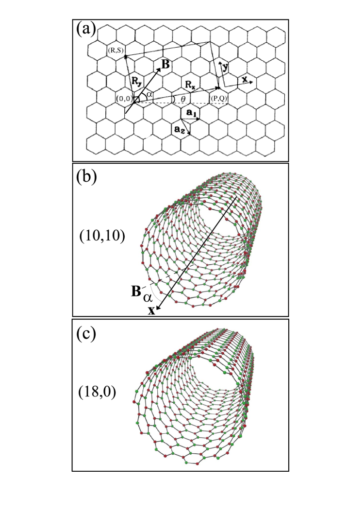
Figure 34: Geometric structures for (a) graphene $\&$ carbon nanotubes; (b) (10,10) $\&$ (18,0) nanotubes. Also shown in (b) is the relation between nanotube axis and magnetic field.

However, their abnormal $B_{0}$-dependent properties are exhibited by perturbed LLs in small anticrossing-LL regions, as shown in the dashed green ellipse in Fig. 34 (b). The corresponding peak intensities and frequencies are discontinuous as a function of $B_{0}$ and extra optical selection rules are induced for such LLs with hybridized quantum modes. The larger the layer number N is, the more complex the absorption spectrum will be. Furthermore, the spectrum can’t converge to 3D spiral-Dirac absorption spectrum due to the absence of $\overline{P}3m$ symmetry in the 2D limit.

The identification of the interband transitions is available in magneto-absorption, reflection and transmission measurements. The energy width of double peaks, with a separation of $\sim 10$ meV, can be resolved; besides, it is feasible to probe the Fermi velocity through the measurements of the cyclotron resonance by the far-infrared spectroscopy. Moreover, near the Fermi level, rhombohedral graphite has bulk gaps between the low-lying LSs in a very weak magnetic field (estimated in Eq. (58)). The achievement of 3D QHE is attainable within the region of bulk gaps; the expected QHE plateaus are different than the experiments reported in ABC-stacked trilayer graphenes.[40] Furthermore, this is in contrast to the cases of AA- and AB-bulk graphite which owns unattainable field strengths that are required to open the bulk gaps to observe a series of 3D QHE plateaus.

6 Quantum confinement in carbon nanotubes and graphene nanoribbons

The periodical boundary condition in a cylindrical nanotube surface can quantize the electronic states with the angular momenta (${J^{c,v}}$’s) corresponding to the well-behaved standing waves. This leads to a specific optical selection rule, when the electric polarization is parallel to the surface.[234, 235, 141, 142, 143, 144] The cooperation with magnetic field greatly enriches the fundamental properties. Magneto-electronic and optical spectra are very sensitive to the changes in the magnitude and direction of magnetic field and the nanotube geometry (radius and chiral angle). The ${\bf B}$-field can create the metal-semiconductor transition, drastically change the 1D energy dispersions, obviously destroy the state degeneracy, and induce the coupling of different angular momenta. As a result, there are more ${\bf B}$-dependent absorption peaks in the square-root asymmetric form. Specifically, the magnetic quantization, with high state degeneracy, is absent except for very large radii and strong fields.

On the other hand, a finite-size graphene nanoribbon does not have a transverse wave vector, owing to the open boundary condition. The nanoribbon width, edge structures, and external field are responsible for the unusual properties. It is predicted to present the edge-dependent optical selection rules in terms of the subband indices (${J^{c,v}}$’s).[139, 138, 140] By the detailed analyses, they principally come from the peculiar spatial distributions of the edge-dominated standing waves. A perpendicular magnetic field could result in QLLs, while the magnetic length is longer than the nanoribbon width. Each QLL is composed of the partially flat and parabolic dispersions. It dramatically changes the main features of electronic and optical spectra. The magneto-optical selection rule of QLLs is similar to that of monolayer graphene. Graphene nanoribbons are quite different from carbon nanotubes in quantum numbers, wave functions, energy gaps, state degeneracies, selection rules, and magnetic-field effects, clearly illustrating the critical roles of the boundary conditions.

6.1 Magneto-electronic properties of carbon nanotubes

Each carbon nanotube can be constructed from by rolling up a graphene from the origin to the lattice vector ${{\bf R_{x}}=P{\bf a_{1}}+Q{\bf a_{2}}}$, where ${\bf a_{1}}$ and ${\bf a_{2}}$ are primitive lattice vectors of a 2D sheet (Fig. 35 (a)). A ($P$,$Q$) nanotube has a chiral angle of ${\theta\,=tan^{-1}[\sqrt{3}\,Q/(2P+Q)]}$ and radius of ${r=b\sqrt{3(P^{2}+PQ+Q^{2})}/2\pi}$. ($P$,$P$) and ($P$,0), respectively, correspond to nonchiral armchair and zigzag systems (${\theta\,=30^{\circ}}$ and $0^{\circ}$). The number of carbon atoms in a primitive unit cell is $N_{c}=4\sqrt{(P^{2}+PQ+Q^{2})(R^{2}+RS+S^{2})/3}$, where $(R,S)$ correspond to the primitive lattice vector along the nanotube axis.

The misorientation of 2$p_{z}$ orbitals (the curvature effect) on the cylindrical surface leads to the change in the hopping integral, i.e., $\gamma_{i}$=$V_{pp\pi}$ $\cos$($\Phi_{i}$)+$4(V_{pp\pi}-V_{pp\sigma}$) [${r}/{b}$ $\sin^{2}$(${\Phi_{i}}/{2}$)]², where $i$(=1, 2, 3) corresponds to the three nearest neighbors, and $\Phi_{i}$ ($\Phi_{1}=-b\cos(\pi/6-\theta)/r$, $\Phi_{2}=b\cos(\pi/6+\theta)/r$; $\Phi_{3}=-b\cos(\pi/2-\theta)/r$) represents the arc angle between two nearest-neighbor atoms. The Slater-Koster parameters $V_{pp\pi}$$(=-2.66$ eV) and $V_{pp\sigma}$$(=6.38$ eV), respectively, represent the $\pi$ and $\sigma$ bondings between two $2p$ orbitals in a graphene plane.[240] The Hamiltonian matrix will be built for any magnet-field directions. $\alpha$ is the angle between magnetic field and axis. As for a zero or parallel magnetic field, a ${2\times\,2}$ Hamiltonian, accompanied with ${J^{c,v}=1,2,3...;N_{c}/2}$, is sufficient in calculating the essential properties.[239] On the other hand, the different J’s would couple one another as the magnetic field deviates from the nanotube axis. The perpendicular component $B_{\perp}=B_{0}=\sin\alpha$ leads to the J coupling and the total carbon atoms in a primitive cell are included in the tight-binding calculations (details in [238, 143]).

Each carbon nanotube has a lot of 1D energy subbands at zero field, being defined by angular momenta of ${J^{c,v}}$’s, as shown in Fig. 36. For a ${(P,P)}$ armchair nanotube, a pair of linear valence and conduction bands, with ${J^{c,v}=P}$, intersects at ${E_{F}=0}$, e.g., those of ${J^{c,v}=50}$ in (50,50) nanotube (gray-dotted curves in Fig. 36(a)). They create a finite DOS there (Fig. 38(a)) and thus behave as a 1D metal. That the metallic behavior is not affected by the curvature effect could be identified from the periodical boundary condition and the specific changes of the nearest-neighboring hopping integrals.[131] That is, the Fermi-momentum states in armchair carbon nanotubes are sampled from the Dirac points of a graphitic sheet. In addition, the misorientation of ${2p_{z}}$ orbitals only leads to a slight redshift in the Fermi momentum ($k_{F}$), compared with 2/3 (in unit of ${\pi\,/I_{x}}$; $I_{x}$ the periodical distance along the nanotube axis). The higher/deeper energy subbands are doubly degenerate, since they correspond to ${J^{c,v}}$ and ${N_{c}/2}-{J^{c,v}}$ simultaneously. They present parabolic dispersions near the band-edge state of ${k_{x}=k_{F}}$.

The radius and chiral angle can determine energy gap and state degeneracy. ${(P,Q)}$ carbon nanotubes, respectively, belong to narrow- and moderate-gap semiconductors, being characterized by ${(2P+Q=3I}$ $\&$ ${P\neq\,Q)}$ and ${2P+Q\neq\,3I}$. The former and the latter, with energy gaps inversely proportional to radius and square of radius, arise from the periodical boundary condition and the curvature effect, respectively.[239, 131] For example, the narrow-gap ${(90,0)}$ and ${(80,20)}$ nanotubes and the moderate-gap ${(91,0)}$ nanotube, respectively, have ${E_{g}\sim\,0.0005}$ $\alpha_{0}$ (Figs. 36(b) and 36(d)) and 0.03 $\alpha_{0}$ (Fig. 36(c)). In general, the low-lying valence and conduction bands in semiconducting nanotubes possess the parabolic dispersions with double degeneracy.

State degeneracy, band gap and energy dispersions strongly depend on the direction and strength of a uniform magnetic field. When ${\bf B}$ is parallel to the nanotube axis, the angular momentum becomes ${{J^{c,v}}+\phi\,/\phi_{0}}$ (magnetic flux ${\phi\,=\pi\,r^{2}B_{0}}$). The gapless linear bands of armchair nanotubes are changed into the separate parabolic bands (black-dotted curves in Fig. 36(a)), i.e., the metal-semiconductor transition occurs in the presence of $\phi$. Furthermore, the magnetic flux destroys the double degeneracy in the higher/deeper energy subbands; that is, two subbands characterized by the angular momenta of ${J^{c,v}}$ and ${N_{c}/2-J^{c,v}}$ are not identical to each other because of the magnetic splitting effect. Such effects are relatively prominent, when the direction of magnetic field approaches the nanotube axis. On the other hand, a non-parallel magnetic field will result in the coupling of different ${J^{c,v}}$’s, being stronger at large $r$, ${B_{0}}$ and $\alpha$. Specifically, a perpendicular magnetic field can break the state degeneracy, in which the spitting subbands are symmetric about ${k_{x}=2/3}$ (green-dotted curves). An armchair nanotube keeps the metallic bahavior at ${\alpha\,=\pi\,/2}$. Whether the intersecting linear energy bands become the gapless parabolic ones depend on radius and field strength. For example, (50,50) and (100,100) nanotubes, respectively, exhibit the linear and parabolic dispersions (green- and orange-dotted curves). Moreover, the ${\bf B}$-induced effects on band structures are clearly revealed in non-armchair carbon nanotubes (Figs. 36(b)-36(d)).

There exist the diverse relations between energy gap and magnetic field. Under a parallel magnetic field, energy gaps present a linear and non-monotonous relation with a period of ${\phi_{0}}$, as clearly indicated in Fig. 37. $E_{g}$ of an armchair nanotube grows in the increase of $\phi$, reaches a maximum value at ${\phi\,=\phi_{0}\,/2}$, and then recovers to zero at ${\phi_{0}}$ (black curve in Fig. 37(a)). The metal-semiconductor are also revealed in the narrow- and middle-gap carbon nanotubes (black curves in Figs. 37(b) and 37(c)) near small $\phi$ and ${\phi_{0}\,/3}$ (or $\phi_{0}$ $\&$ ${2\phi_{0}\,/3}$). In addition, they might be absent in part of narrow-gap systems (inset in Fig. 37(d)). Obviously, the periodical Aharonov-Bohm effect is presented in energy gaps of any carbon nanotube. It would be very difficult to observe this effect in the presence of a dominating perpendicular magnetic field, e.g., ${E_{g}}$’s at large ${\alpha}$’s. There are no simple relations between energy gaps and $\phi$ under the non-parallel fields. As for the middle-gap nanotubes (Fig. 47(c)), the larger is $\alpha$, the higher is the $B_{0}$-field strength of the semiconductor-metal transition. Specifically, at ${\alpha\,=90^{\circ}}$, both armchair and narrow-gap nanotube keep the gapless feature (green curves in Figs. 37(b) $\&$ 37(d)), i.e., the metal-semiconductor transition does not happen during the variation of field strength. The predicted strong dependence of energy gap on the strength and direction of magnetic field and the nanotube geometry could be further verified from the STS measurements.

The special structures in DOS are greatly enriched by the nanotube geometry and the magnetic-field direction, as shown in Fig. 38. The 1D band-edge states in parabolic and linear dispersions, respectively, create the square-root asymmetric peaks and plateaus. All VHSs belong to the former except for that near ${E=0}$ in metallic nanotubes at zero field (gray solid curve in Fig. 38(a)). For an armchair nanotube, a parallel magnetic field makes the plateau change into a pair of asymmetric peaks with an energy gap (black curve), and the number of the intensity-reduced asymmetric peaks at other energies becomes double. The energy spacing between two neighboring peaks declines as ${\alpha}$ grows (red, blue and green curves). Furthermore, they are merged together under a perpendicular field (green (orange) curve), in which there is a plateau structure (a symmetric peak) near ${E=0}$ because of a pair of gapless linear (parabolic) bands (Fig. 36(a)). Compared with metallic armchair nanotubes, the narrow-gap systems, as shown in Figs. 38(b) and 38(d), present the almost same structures except for a pair of very close asymmetric peaks near the Fermi level at zero field (insets). However, there are more peaks structures in the moderate-gap nanotubes (Fig. 38(c)). On the experimental side, the zero-field DOS characteristics, including the asymmetric peaks, the energy spacings, the metallic behaviors,[193, 194] and the middle and narrow gaps,[132] have been verified by the STS measurements. The rich peak structures and the metal-semiconductor transitions due to a uniform magnetic field require further experimental verifications on DOS.

6.2 Magneto-optical spectra of carbon nanotubes

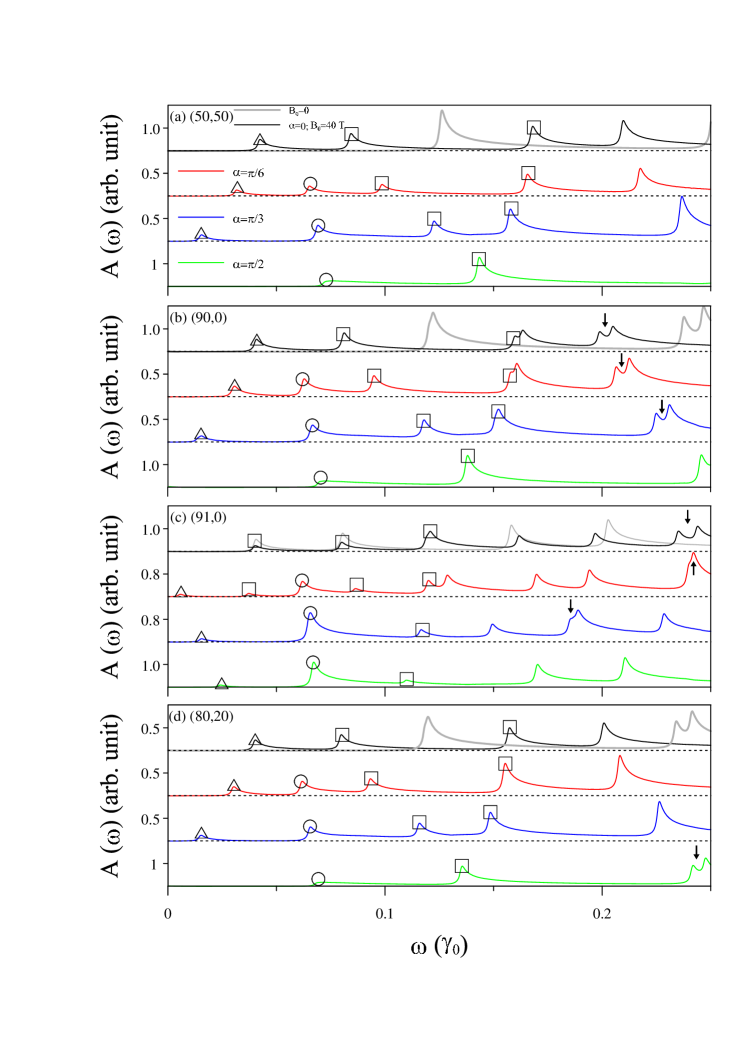
Figure 39: Optical absorption spectra of (a) (50,50), (b) (90,0), (c) (91,0) and (d) (65,35) carbon nanotubes under zero field and various magnetic-field directions.

The standing waves on a cylindrical surface plays a critical role in determining the available optical excitation channels. At zero field, they present the well-behaved spatial distributions, with the forms of sine/cosine functions closely related to the angular momenta, as revealed in Figs. 39(a)-39(c). For an armchair nanotube, the linear energy bands possess a uniform distribution along the azimuthal direction (gray curves in Fig. 39(a)), and the higher-energy bands correspond to the normal oscillations of one, and two wavelengths (Figs. 39(b) and 39(c)). Such features are independent of $k_{x}$ s and keep the same in the presence of a uniform magnetic field, leading to the identical optical selection rule at zero and parallel magnetic fields. In addition, these two factors only create the rigid shifts in the azimuthal distributions. As to the non-parallel magnetic fields, the normal standing waves are changed into the distorted ones, especially for a perpendicular one (green curves in Figs. 39(a)-39(c)). However, the latter could be regarded as a superposition of the $J$-decoupled normal modes, since a perpendicular field creates the coupling of distinct angular momenta. It is relatively easy to observe the coupling effect in larger nanotubes. For example, an armchair (100,100) nanotube exhibits the highly distorted standing waves with more zero points (orange curves in Figs. 39(e) and 39(f)), corresponding to the gapless parabolic energy bands near ${E_{F}}$ and the oscillatory ones (Fig. 36(a)).

The electric polarization is assumed to lie on the nanotube surface (parallel to the nanotube axis), as considered in layered graphites (Eq. (38)). All the carbon nanotubes only exhibit the asymmetric absorption peaks in the square-root form, as shown in Fig. 40. The available excitation channels arise from the occupied valence subbands and the unoccupied conduction ones, with the same angular momentum. The selection rule of ${\Delta\,J=J^{v}-J^{c}=0}$ is determined by the $J$-decoupled standing waves. It could be further applied to any magnetic fields even with the coupling of $J$’s by using the superposition of distinct components. At zero field (gray curve in Fig. 40(a)), an armchair nanotube does not have the threshold absorption spectrum, since the vanishing velocity matrix elements (Eq. (39)) prevent the interband excitations due to a pair of linearly intersecting energy bands. The featureless optical spectrum is also revealed in monolayer graphene (Fig. 4(b)). The absorption peaks are closely related to the band-edge states of the parabolic valence and conduction bands; that is, absorption frequency is their energy spacing. The weaker is the energy dispersion, the stronger is the asymmetric peak.

The number, frequency and intensity of absorption peaks are very sensitive to the magnetic field. The threshold absorption peak of an armchair system is generated by a parallel magnetic field (triangle related to the black curve in Fig. 40(a)). The number of other absorption peaks becomes double (two rectangles) and their intensities are getting weak, directly reflecting the splitting of the $J$-dependent degeneracy (Fig. 36(a)). All the absorption peaks agree with the ${\Delta\,J=0}$ rule. This rule is also suitable for most of peak structures even when a magnetic field gradually deviates from the nanotube axis. The first peak declines quickly and two neighboring peaks approach to each other (red and blue curves), in which the former disappears and the latter change into a single peak under a perpendicular magnetic field (green curve). It should be noticed that the absence of threshold peak at ${\alpha\,=\pi\,/2}$ is independent of the radius of armchair nanotube and field strength. On the other hand, there exists an extra low-frequency absorption peak (circle in red, blue and green curves), mainly owing to the vertical excitations of the first (second) valence band and the second (first) conduction band (Fig. 36(a)). This peak does not satisfy the selection rule of ${\Delta\,J=0}$, while it could be identified from the coupling of the neighboring angular momenta.

The main features of absorption peaks strongly depend on the geometric structures of carbon nanotubes. The narrow-gap systems exhibit a zero-field threshold peak at very low frequency (insets in Figs. 40(b) and 40(d)). For a non-perpendicular $B_{0}$-field, they might have the merged double-peak structures (arrows in Fig. 40(b)), reflecting the small energy spacings between two neighboring parabolic subbands with high DOSs (Fig. 37(b)). In addition, an extra prominent magneto-absorption peak of ${\Delta\,J\neq\,0}$ is revealed in all carbon nanotubes at ${\alpha\neq\,0^{\circ}}$ (circles in Fig. 37) because of the coupling of distinct angular momenta. As for the moderate-gap nanotubes, there are more prominent absorption peaks (Fig. 40(c)) arising from the rich low–lying parabolic subbands (Figs. 36(c) and 37(c)).

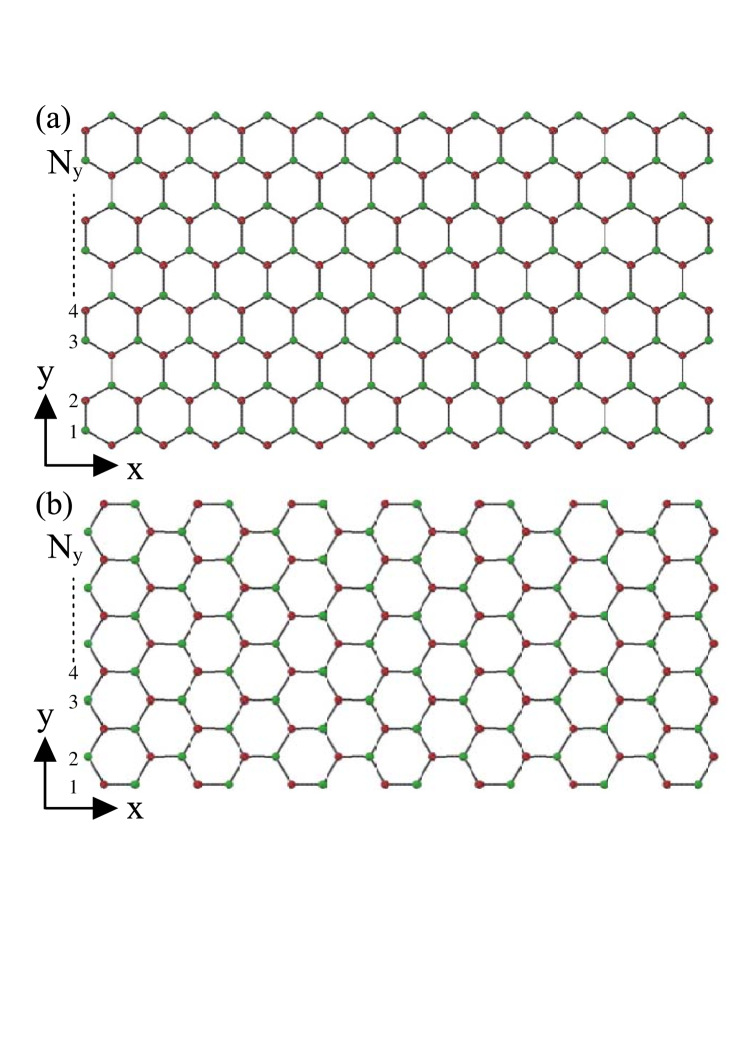
Figure 41: Geometric structures of (a) zigzag and (b) armchair graphene nanoribbons. $N_{y}$ is the number of zigzag or dimer lines.

The dependence of absorption frequencies on the magnetic-field direction is important in understanding the characteristics of prominent peaks, mainly owing to the composite effects arising from the splitting and coupling of angular momenta. For example, within the frequency range of ${\omega\leq\,0.25}$ $\gamma_{0}$, all the magneto-absorption peak frequencies monotonously grow or decline as the magnetic field gradually deviates from the nanotube axis, as clearly shown in Fig. 41. This is related to the band-edge state energies of the split subbands. The transition intensities will present the drastic change during the variation of ${\alpha}$, so that absorption peaks might disappear or come to exist. The threshold peak (triangle) becomes absent in the metallic (narrow-gap) carbon nanotubes under a large ${\alpha}$, e.g., ${\alpha\,=86^{\circ}}$ for (50,50) nanotube in Fig. 41(a). However, it could survive in the middle-gap systems for any angles (Fig. 41(b)). Its disappearance and existence, respectively, correspond to the intersecting linear bands and the gapped parabolic bands (green curves in Figs. 36(a) and 36(c)). An extra peak (circle), reflecting the significant coupling effect, is revealed at a enough large $\alpha$ (${\sim\,3.6^{\circ}-5.4^{\circ}}$). Most of magneto-absorption peaks (rectangles) present the splitting behavior. Whether they are merged together or become absent depends on $\alpha$. Up to now, the splitting peaks due to a parallel magnetic field have been confirmed by the optical measurements.[145] The predicted strong dependence on the magnetic-field direction and the nanotube geometry is worthy of further examinations.

6.3 Magneto-electronic properties of graphene nanoribbons

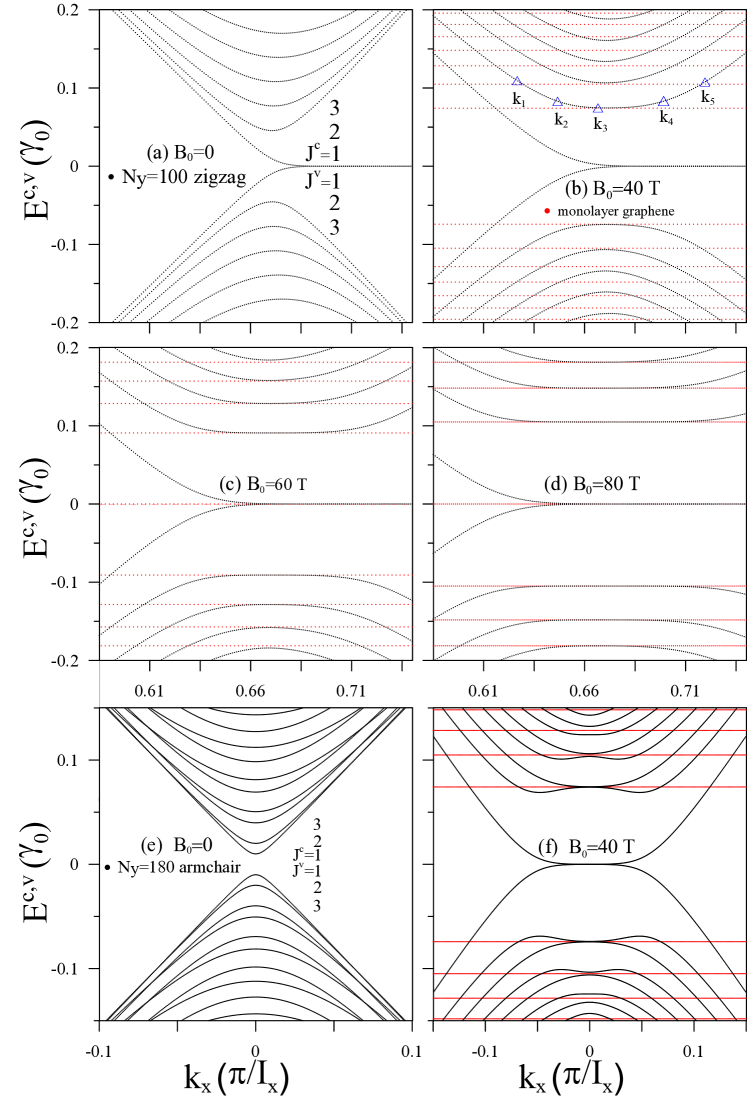
Figure 42: Band structures of a ${N_{y}=100}$ zigzag nanoribbon at (a) ${B_{0}=0}$, (b) ${B_{0}=40}$ T, (c) ${B_{0}=60}$ T; (d) ${B_{0}=80}$ T, and those of a ${N_{y}=180}$ armchair nanoribbon at (e) ${B_{0}=0}$; (b) ${B_{0}=40}$ T. The red lines represent the LL energies of monolayer graphene. ${J^{c,v}}$ is the subband index, as measured from the Fermi level.

Two typical kinds of achiral graphene nanoribbons, with the hexagons normally arranged along the edge structure, are chosen for a model study. Zigzag and armchair graphene nanoribbons, respectively, correspond to armchair and zigzag carbon nanotubes. Their widths could be characterized by the numbers of zigzag and dimer lines ($N_{y}$) along the transverse $y$-direction, respectively (Figs. 42(a) and 42(b)). The low-energy band structures are evaluated from the ${2N_{y}}$ tight-binding functions of ${2p_{z}}$ orbitals. Such functions are combined with the Peierls phases to explore the magneto-electronic and optical properties. For a zigzag ribbon, the Peierls-tight-binding Hamiltonian matrix can be expressed as:

$$H_{ij}=\ \ \left\{\begin{array}[]{cc}2\gamma_{0}\cos(k_{x}\frac{\sqrt{3}b}{2}+\Delta{G}_{1})&\\ \gamma_{0}&\\ 0&\end{array}\begin{array}[]{c}\text{for}\\ \text{for}\\ \text{others,}\end{array}\begin{array}[]{ccc}\text{j=i+1,}&\text{j}&\text{is even,}\\ \text{j=i+1,}&\text{j}&\text{is odd,}\\ &&\end{array}\right.$$ (66)

where the Peierls phase difference $\Delta{G}_{1}=-\pi\phi(j/2-[N_{y}+1]/2)$.

As to an armchair ribbon, the Hamiltonian matrix is given by

$$H_{ij}=\ \ \left\{\begin{array}[]{cc}\gamma_{0}\exp i(-k_{x}b+\Delta{G}_{1})&\\ \gamma_{0}\exp i(k_{x}b/2+\Delta{G}_{2})&\\ \gamma_{0}\exp i(-k_{x}b/2+\Delta{G}_{3})&\\ 0&\end{array}\begin{array}[]{c}\text{for}\\ \text{for}\\ \text{for}\\ \text{others,}\end{array}\begin{array}[]{ccc}\text{j=i+1,}&\text{j}&\text{is even,}\\ \text{j=i+3,}&\text{j}&\text{is even,}\\ \text{j=i+1,}&\text{j}&\text{is odd,}\\ &&\end{array}\right.$$ (67)

where $\Delta{G}_{1}=\pi\phi(j/2-[N_{y}+1]/2)$, $\Delta{G}_{2}=-\pi\phi/2(j/2-1-[N_{y}]/2)$ and $\Delta{G}_{3}=\pi\phi/2[(j+1/2)-1-[N_{y}]/2]$.

The dimension of Hamiltonian keeps the same even in the presence of a perpendicular magnetic field, while it is largely enhanced for layered graphenes[224] or graphites (Chap. 2). The strong competition between the finite-size confinement and the magnetic quantization will greatly diversify the essential properties.

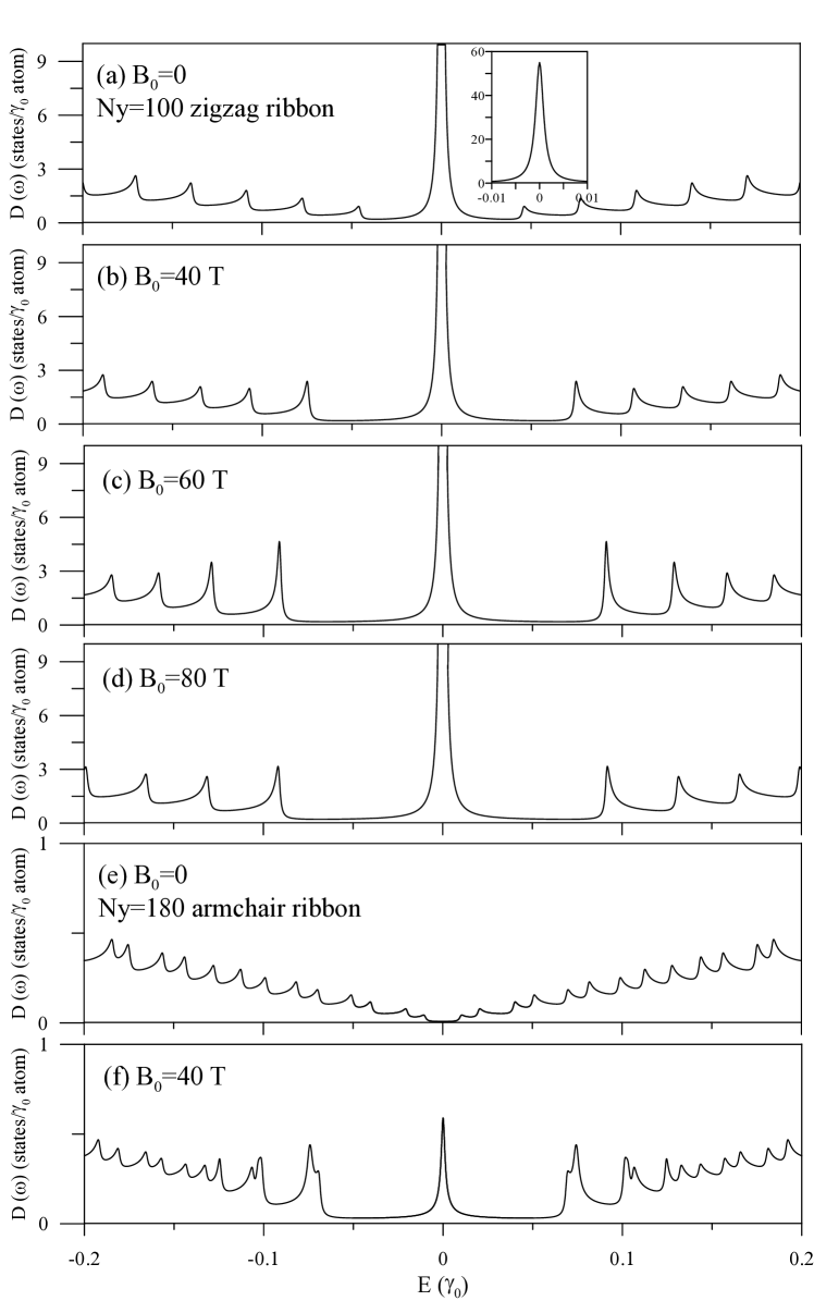
Figure 43: Density of states corresponding to electronic structures in Fig. 42.

The finite-size effect directly induces a plenty of 1D energy subbands, as shown in Fig. 43. Each subband does not have a transverse quantum number under the open boundary condition; furthermore, the ${J^{c,v}}$ index only represents the arrangement ordering measured from the Fermi level. This is one of the most important differences between graphene nanoribbons and nanotubes. Electronic structures strongly depend on the edge structures. A ${N_{y}=100}$ zigzag nanoribbon exhibits the band-edge states near ${k_{x}=2/3}$ (Fig. 43(a)), being similar to those in a ${(50,50)}$ armchair nanotube (Fig. 36(a)). All the low-lying energy subbands possess the parabolic dispersions except for the first pair with the partially flat ones at larger $k_{x}$’s. The latter belong to the edge-localized states (discussed later). On the other hand, the band-edge states are situated at ${k_{x}=0}$ for an armchair nanoribbon e.g., ${N_{y}=180}$ in Fig. 43(e). Each energy subband has no double degeneracy except for the spin degree of freedom. The energy gap, which is determined by the parabolic valence and conduction subbands of ${J^{c,v}=1}$, declines in the increase of ribbon width. The width-dependent energy gaps have been confirmed by the STS measurements.[134, 135, 136, 137]

The energy dispersions are dramatically changed by the magnetic quantization. The energy spacings of a zigzag nanoribbon are getting nonuniform during the variation of $B_{0}$, as shown for ${N_{y}=100}$ in Fig. 43(b) at ${B_{0}=40}$. When field strength is enough high, the lower-energy 1D parabolic subbands will evolve into the composite subbands (QLLs) with the parabolic and dispersionless relations simultaneously, e.g., ${J^{c,v}=2}$ and 3. A sufficiently large nanoribbon width, being comparable to or longer than the magnetic length (${l_{B}}$), accounts for the creation of QLLs. With a further increase of field strength, the dispersionless $k_{x}$-ranges become wider, and the higher-energy subbands might be transformed into the QLLs, such as magneto-electronic structures in Figs. 40(c) and 40(d) at ${B_{0}=60}$ and 80 Ts, respectively. Specifically, the initial energies of QLLs will approach to the LL ones in monolayer graphene (red lines; the 2nd term in Eq. (43)). These clearly indicate that electronic states are gradually quantized into Landau modes from the lower-energy subbands with the increasing $B_{0}$, since they have the smaller kinetic energies. It is relatively easy to observe the dispersionless Landau states under the enhanced field strength and the extension of nanoribbon width. The formation centers of QLLs, respectively, correspond to ${k_{x}=2/3}$ and 0 for zigzag and armchair nanoribbons (Fig. 40(f) at 40 T). It should be noticed that two neighboring subbands of the latter will gradually approach to each other in the increase of $B_{0}$, covering the gradual couplings of (${J^{c}=1,J^{v}=1}$), (${J^{c}=1,J^{v}=1}$) and (${J^{v},J^{v}+1}$). As a result, magneto-electronic structures of armchair nanoribbons might behave as the splitting QLLs except for the pair of valence and conduction QLLs. There exist the extra band-edge states and energy gap is vanishing under a strong magnetic field.

DOSs of the 1D energy subbands present a lot of asymmetric peaks in the square-root form, as clearly indicated in Fig. 44. The peak height, which is inversely proportional to the square-root of subband curvature, grows as state energy increases. It is remarkable that the peak spacings are almost uniform in zigzag system (Fig. 44(a)), but non-uniform in armchair one (Fig. 44(e)). Specifically, the former has a pair of merged peaks near ${E=0}$ or an obvious symmetric peak there (inset in Fig. 44(a)). The low-lying asymmetric peaks become the delta-function-like symmetric ones, when the QLLs could be created by a $B_{0}$-field (Figs. 44(b), 44(c), 44(d) and 44(f)). Furthermore, their heights decline quickly in the increase of QLL energy, reflecting the diminish of the dispersionless $k_{x}$-ranges (Fig. 43). Under the increasing field strength, all the peak energies are enhanced for zigzag systems, while a simple dependence is absent for armchair ones.⁶¹ As a result, QLLs of the former will recover to LLs of monolayer graphene if the magnetic field plays a dominating role (Figs. 43(b)-43(d)). The latter could exhibit the complex structures covering single and double peaks.

6.4 Magneto-optical spectra of graphene nanoribbons

When electrons are confined in the finite-width nanoribbons, their spatial distributions reveal as the regular standing waves (Fig. 45). The oscillatory patterns, with the specific number of nodes, are very sensitive to the edge structures, sublattices, state energies, and wave vectors. They are quite different from those in carbon nanotubes (Fig. 38), and so do the optical properties. For zigzag nanoribbons, the wave functions could be decomposed into the subenvelope functions on the A and B sublattices at the odd and even zigzag lines (Figs. 45(a)-45(c)). The spatial distributions of wave functions present the alternative change between the symmetric and anti-symmetric forms as the subband index increases (more detailed relations in Ref. 41). On the other hand, those of armchair systems lie at the ${3m}$-, ${(3m+1)}$-, and ${(3m+2)}$-$th$ dimer lines of the A and B sublattices (Fig. 45(d)-45(f)). There are two kinds of unique relations. For a specific subband, the subenvelope functions on two sublattices possess the same phase or the phase difference of $\pi$. Furthermore, the valence and conduction subbands, with the identical index, exhibit the similar phase relation in the subenvelope functions of the A ($B$) sublattice. It is very significant that the special relations in wave functions are edge-dependent and thus dominates the distinct selection rules. However, the main features of the angular-momentum-dominated standing waves in carbon nanotubes (Fig. 39) are independent of the chiral angle.

A dominating magnetic field can thoroughly alter the characteristics of wave functions, regardless of the edge structures. In general, the standing waves are changed into the well-behaved LL wave functions, as clearly indicated in Figs. 46(a)-46(e) for a zigzag system. The ${k_{x}=2/3}$ states present the symmetric or anti-symmetric distributions about the nanoribbon center. They are identical to those of monolayer graphene (Fig. 5(b)) except that the first pair of QLLs possesses the edge-localized distributions (Fig. 46(c) and 46(d)). With the different wave vectors, the spatial distributions, being revealed in Figs. 46(f)-46(j), are getting asymmetric. Furthermore, the number of zero points might be lost as the wave vectors are far away from ${2/3}$. Apparently, the competition between magnetic quantization and finite-size confinement will lead to the coexistent behavior, in which LL modes and standing waves, respectively, correspond to low- and high-lying electronic states. This unusual feature could be observed by changing the $B_{0}$-field strength or nanoribbon width.

Graphene nanoribbons possess the edge-dependent optical selection rules, as shown in Fig. 47. The optical vertical excitations arise from the interband transitions of the $J^{v}$-th valence band and the $J^{c}$-th conduction band. For zigzag nanoribbons, a lot of asymmetric absorption peaks in the square-root form are characterized by the selection rule of ${\Delta\,J=2I+1}$ (Fig. 47(a)). The strong absorption peaks might come from the multi-channel excitations simultaneously, especially for the higher-frequency ones. This rule could be directly derived from the non-vanishing velocity matrix elements (Eq. (39)) by using the special relations in the subenvelope functions (detailed calculations in Ref. 41). On the other side, the available excitation channels in armchair systems agree with the $\Delta J=0$ rule, so the number of absorption peaks is reduced. The valence and conduction bands, with the identical $J$, could also be revealed as the prominent absorption peaks of any carbon nanotubes (Fig. 40), while the angular momentum is conserved during the vertical transitions.

The unusual transformation between the edge- and QLL-dominated absorption peaks could be presented in the variation of magnetic-field strength (or nanoribbon width), as clearly shown in Figs. 48(a)-48(c). The QLL wave functions have the well-behaved spatial symmetry, so that the effective optical transitions associated with the symmetric absorption peaks are governed by the QLL-dependent selection rule. At lower frequency, the magneto-absorption peaks of ${\Delta\,J\neq\pm\,1}$ are absent or become very weak; furthermore, the ${\Delta\,J=\pm\,1}$ rule is equivalent to the ${\Delta\,n=\pm\,1}$ one in monolayer graphene (red curve in Fig. 48(a)). This is independent of edge structures; that is, the number, frequency and intensity of prominent absorption peaks are identical for zigzag and armchair nanoribbons with the almost same width (Figs. 48(a) and 48(d)). Suck peaks have the symmetric form and stronger intensities at high field strengths (Figs. 48(c) and 48(d)). In addition, some extra lower absorption peaks are revealed by the ${J^{c,v}=1}$ QLLs of the former (e.g., blue circles in Fig. 48(a)) because of the impure LL wavefunctions (Figs. 46(c) and 46(d)), and the splitting QLLs of the latter could create the double-peak structure (blue circles in Fig. 48(d)). Concerning the higher-frequency asymmetric peaks (the right-hand side of the gray-dashed vertical line), there are more prominent structures, especially for the complex absorption peaks in armchair nanoribbons (Fig. 48(d)). They originate from the band-edge states of the parabolic valence and conduction bands, being characterized by the strong competition of the edge- and QLL-dependent selection rules.

The complicated relations among the lateral confinement, magnetic quantization and dimension deserve closer investigations. They could be understood from the initial six prominent magneto-absorption peaks, as clearly revealed in Fig. 49 for their $B_{0}$-dependent frequencies. Zigzag nanoribbons exhibit the monotonic magnetic-field dependence (open circles in Fig. 49(a)). In general, peak frequencies grow with the increasing $B_{0}$ in the absence of a specific relation. They are very different from those of monolayer graphene (red dots) except for the sufficiently high field strength. At low $B_{0}$, the lateral confinement (black circles) dominates the frequency, intensity, form of absorption peaks, e.g., the more higher frequencies compared with the 2D results. It will be seriously suppressed the magnetic quantization, when the field strength is over a critical one (red circles). The number of prominent peaks keeps the same during the variation of $B_{0}$, since the ${\Delta\,J=odd}$-induced peaks (Fig. 47(a)) cover the QLL-created ones. However, absorption peaks in armchair systems might come to exist or disappear frequently as $B_{0}$ gradually increases (Fig. 49(b)), being closely related to the QLL splitting and the high competition of two selection rules. Obviously, a simple $B_{0}$-dependence of magneto-absorption frequencies is absent. The zero-field absorption peaks of ${\Delta\,J=0}$ (black circles; Fig. 47(b)) are not consistent with the ${\Delta\,J=0}$ rule due to the QLLs, so that their intensities decay rapidly and vanish after the critical $B_{0}$s. On the other hand, the new peaks initiated by the strong magnetic quantization might appear in the double-peak structures (two close red-circled curves) or the merged ones. They could behave as the inter-LL peaks in 2D monolayer (red dots) only at higher field strengths. Up to now, there are no optical and magneto-optical measurements on graphene nanoribbons. The theoretical predictions of the edge- and QLL-dominated selection rules could be verified by optical spectroscopies, as done for graphite, layered graphenes, and carbon nanotubes.

6.5 Comparisons and applications

The distinct stacking symmetries in three kinds of layered graphites have created the diverse and novel physical phenomena. The critical differences cover electronic and optical properties in the absence/presence of magnetic quantization. The AA-, AB- and ABC-stacked graphites, respectively, have one, two and one pairs of $\pi$-electronic valence and conduction bands, in which the ${k_{z}}$-dependent band widths are ${\sim\,1}$ eV, ${\sim\,0.1-0.2}$ eV and ${\sim\,0.01}$ eV, and the band-overlap widths near the Fermi level behave similarly. The carrier density of free electrons and holes is highest in simple hexagonal graphite, while it is lowest in rhombohedral graphite. Band structures of three systems could be regarded as the 3D vertical Dirac cone, the composite of monolayer- and AB-bilayer-like ones, and the spiral cone structure. The 3D energy dispersions determine the DOS characteristics, such as, the semi-metallic behavior and van Hove singularity-induced distinct structures. The band-dominated optical spectra exhibit the dimension- and stacking-dependent characteristics at low and middle frequencies, including the frequency, number, form and spectral width of the special absorption structures. The main features of zero-field band structures are directly reflected in the magnetic LSs. In general, the band-edge states of the 1D parabolic LSs are shown as many asymmetric peaks in DOS. AA system exhibits a lot of valence and conduction LSs intersecting with the Fermi level under the specific energy spacings, while ABC system only presents one crossing LS of ${n^{c,v}=0}$. Both of them possess the monolayer-like subenvelope functions and $\sqrt{B_{0}}$-dependent energy spectra. However, AB system has two groups of LSs with the normal and perturbed modes, leading to the coexistence of crossing and anticrossing behaviors. Only the initial two LSs of the first group cross the Fermi level. The $B_{0}$-dependence of LS energies is sensitive to the dimension-induced $k_{z}$, such as the square-root and linear dependences at ${k_{z}=0}$ and $\pi$ (K and H points), respectively. Furthermore, the magnetic subenvelope functions might dramatically change during the variation of $k_{z}$. Specifically, even without any crossings and anticrossings, the rich and unique magneto-optical spectra are revealed by the well-behaved LSs in AA-stacked graphite, including the intraband and interband inter-LS vertical excitations, the Fermi-momenta-induced absorption peaks, the non-uniform peak intensity, the multi-channel threshold peak, intraband two-channel peaks $\&$ interband double-peak structures at distinct frequency ranges, the discontinuous $B_{0}$-dependence of the initial interband channel, and the beating feature related to the vertical Dirac cones. Magneto-absorption peaks agree with the monolayer selection rule of ${\Delta\,n=\pm\,1}$ for AA-, ABC-, and AB-stacked graphites. The second stacking can create the monolayer-like characteristics, such as, the interband transitions, non-composite symmetric peaks due to the same contribution of K and H points, almost uniform intensity, and pure ${\sqrt{B}_{0}}$-dependence of absorption frequency. As for AB-stacked graphite, there are four categories of interband inter-LS excitations arising from the same or different groups. The strong asymmetric peaks might appear at the identical frequency ranges and thus exhibit the very complex absorption structures. Their main features are rather different for the K- and H-point vertical excitations, respectively, leading to the bilayer- and monolayer-like absorption frequencies. Moreover, some extra peaks come to exist under the LS anticrossings. The above-mentioned differences could be examined by the experimental measurements of ARPES, STS and optical spectroscopies on energy bands, DOS, and absorption spectra, respectively.

The dimensional crossover of the essential properties occur in AA- and AB-stacked layered graphenes as the layer number gradually grows. The $N$-layer AA stacking has a vertical multi-Dirac cone structure which is distributed within the $k_{z}$-dependent band width of simple hexagonal graphite. It is a semi-metal under the overlap of valence and conduction bands. However, an optical gap are induced in a $N$-even system, since absorption spectrum is only a combination of $N$ intra-Dirac-cone vertical excitations. Under a perpendicular magnetic field, the magneto-optical gap comes from a forbidden transition region related to the intragroup LLs, and it is greatly enhanced by the increasing field strength. The magneto-threshold channels dramatically changes with the increasing $B_{0}$, in which their intensities are about half of the others. The low-lying Dirac-cone structure, magnetically quantized states, special structures in DOS, and absorption peaks are expected to approach those of AA-stacked graphite for ${N>30}$. As for AB-stacked graphene, band structure of a N-odd system resembles a hybridization of massless Dirac cone and massive parabolic dispersions, while that of a N-even system consists of only pairs of parabolic subbands. When $N$ is very large, the monolayer- and bilayer-like states are expected to correspond to the $H$ and $K$ point in Bernal graphite, respectively. The excitation channels are only allowed between the respective monolayer-like subbands or between the bilayer-like subbands; the magneto-optical selection rule is also applicable to all the inter-LL transitions. With the increase of layer number, the LL anticrossings happen more frequently as compared to those in Bernal graphite. Electron-hole asymmetry-induced twin-peak structures are revealed in both multi-layer and bulk systems. However, in magneto-optical spectrum, the measured profiles of the $B_{0}$-dominated peaks, including threshold channel, intensity, spacing and frequency, could be used to distinguish the stacking layer, configuration and dimension. On the other hand, the dimensional crossover is hardly observed in ABC stacking, mainly owing to the distinct lattice symmetries in 3D and 2D systems. For bulk graphite, a primitive unit cell, rhombohedron, has a bi-particle lattice symmetry. The low-energy electronic properties is described by the 3D anisotropic spiral Dirac cones. Specially, the ABC-stacked graphene possess the surface-localized and sombrero-shaped subbands, irrelevant to the rhombohedral graphite. The zero-field absorption spectrum is contributed by the ${N\times\,N}$ excitation channels of the $N$ pairs of energy bands, in which the low-frequency region is dominated by the surface-localized states. The magneto-optical spectrum consists of ${N\times\,N}$ groups of inter-LL absorption peaks, each of which displays the characteristic $B_{0}$-dependence regarding the frequency, intensity and number. Furthermore, the frequent anticrossing of LLs due to the sombrero-shaped subbands lead to extra peaks which have abnormal relations with the field strength.

The significant effects due to the lateral quantum confinement and magnetic field clearly illustrate the dimension-diversified essential properties. The periodical boundary condition induces the decoupled angular-momentum states in carbon nanotube, but the open one cannot create a transverse quantum number in graphene nanoribbon. The former possesses the sine/cosine standing waves along the azimuthal direction, regardless of radius and chirality. However, the unusual standing waves in the latter depend on edge structure, A and B sublattices; even zigzag and dimer lines. The distinct characteristics of subenvelope functions dominate the diverse selection rules, the conservation of angular momentum in carbon nanotube, the same index of valence and conduction subbands in armchair nanoribbons, and the index difference of odd integers in zigzag nanoribbons. All the special structures in DOS and absorption spectrum are presented in the asymmetric peaks of square-root form. The magnetic quantization in cylindrical nanotubes is mainly determined the field direction and strength. A parallel magnetic field leads to the shift of angular momentum or the destruction of double degeneracy, and the periodical Aharonov-Bohm effect in energy dispersions, band gaps and absorption peaks. However, the discrete angular momenta are coupled with one another in the presence of a perpendicular magnetic field, and QLLs hardly survive in cylindrical systems except for very high field strength and large radius. Apparently, optical spectra are dramatically altered by the magnetic field, such as, more splitting peaks with the same rule and some extra peaks without the optical rule under the parallel and perpendicular ones, respectively. On the other hand, QLLs could exist in graphene nanoribbon if the width is sufficient for the localized oscillatory distribution. Their dispersionless $k_{x}$-ranges can transform the asymmetric peaks of DOS and absorption spectrum into the symmetric ones. Moreover, the latter and the former, which correspond to the QLL- and edge-dependent selection rules, respectively, appear at the lower and higher frequencies.

Graphite, as well as graphite intercalation compounds, have been extensively developed for various applications during a long tome as a result of the unique properties. Pristine graphite is a suitable precursor in the production of other carbon-related materials. It is the most stable allotrope of carbon. The covalent bondings between C atoms in the same layer can create graphite’s high temperature stability, and excellent electrical and thermal conductivity. Owing to the superior mechanical properties, graphite fibers are frequently utilized for reinforced composite materials[242, 243, 244, 245]. Graphite intercalation compounds, with the significant chemical bondings between adatoms and carbons, exhibit wide applications in electronics[246, 247], energy storage[248] and electrochemistry[249, 250]. The most common use in industry serves as a low-cost electrode.[251, 252] The high free electron (hole) density is generated by the intercalation of metal atoms (molecules).[241] The metallic compounds could be used as superconductors with high transition temperatures. e.g., 11.5 K for C₆Ca and C₆Yb.[258, 259, 12] They have also been applied for photo electro catalytic, electrochemical and biomedical sensor[256, 257, 255, 253, 254]. Graphite composites display high conductivity for microbial fuel cells applications in electrochemistry[261, 262, 260]. The field-effect transistor (FET) sensor based on graphite oxide nanoparticle composites presents an advantage of low cost and possesses high selectivity and excellent stability.[263, 264]

Graphene-related materials have displayed the high potentials for electronic, photonic and optoelectronic applications, such as touch-screen panel device,[266, 267] light-emitting diodes (LEDs)[268, 269, 270, 271, 272], solar cells,[276, 275, 274, 273] photo-detectors[283, 284, 282, 281, 279, 277, 278, 280] and photo-modulators.[285, 286] The direct application of graphene in FETs is suppressed owing to its zero-gap nature. However, bilayer graphene can open a sizable and tuneable bandgap by applying a gate voltage, which is appropriate for making large-area graphene FETs with extremely thin, shorter and higher speeds channels.[287, 288, 289, 290] The high transparency and flexibility of graphene could be utilized to design thin, light and delicate devices[268, 269]. Graphene-based optical modulator possesses great advantages in low operation voltage, fast modulation speed, small footprint and large optical bandwidth, compared with semiconductor ones[285, 286]. By tuning the Fermi level or the free carrier concentration of graphene sheets, the modulator is operated over a broad wavelength range. As a result of the strong and rich interband optical transitions, the graphene detectors are suitable for the applications within a very wide energy spectrum, covering the ultraviolet, visible, infrared and terahertz frequency ranges[285, 286]. When layered graphenes are further doped with adatoms or molecules, they might change into gap-modulated semiconductors or metals. Specifically, graphene oxides and hydrogenated graphenes possess the adatom-modulated energy gaps in a wide range of ${0<E_{g}<4.0}$ eV, depending on the concentration and distribution of adatoms.[291, 292] The tunable and controllable electronic properties make them serve as potential candidates, such as FETs,[293, 294, 295]; supercapacitors,[296, 297] sensors,[298, 299] photovoltaic[300, 301, 302] and light-emitting devices.[302, 303] The alkali- and Al-induced high free carrier density might have high potentials in future technological applications, e.g., high-capacity batteries,[304, 305] and energy storages.[306, 307]

The wide-range applications in electronic devices have been made with carbon nanomaterials, such as 1D carbon nanotubes[312, 310, 311, 265] and graphene nanoribbons,[265, 6] 2D few-layer graphene[265] and 3D graphites.[246, 247, 248, 251, 252, 253, 254, 256, 257, 258, 259, 12, 255] Up to now, FET based on semiconducting nanotubes and nanoribbons are widely developed, mainly owing to the advantage of high mobility under the low scatterings. In carbon nanotubes, the intrinsic 1D electronic structures, with the decoupled states of angular momenta, dominate the 1D quantized electrical properties, including the radius-dependent resistance, capacitance and inductance, which are diameter dependent and responsible for the non-monotonic dependence of the electrical mobility.[308] The first FETs made of carbon nanotubes were reported in 1998,[310, 311] which have superior electrical properties of the conducting channels by the gate-voltage modulation. The nano-scaled carbon nanotubes are responsible for low scatterings and allows the gate’s ability to control the potential of the channel in the ultimate thin FETs, while suppressing short-channel effects.[311, 312] Moreover, semiconducting nanotubes present wide applications on optoelectronic devices, such as electroluminescent light emitters,[313, 314] supercapacitors[315] and photodetectors.[281, 282, 283]. Both electrons and holes confined on the cylindrical surface are driven towards each other by applying the appropriate biases on source and drain of the FET. The recombination due to the two types of excited carriers emits electroluminescence, and the photon-emission process is extensively utilized in LEDs.[318, 317, 316] The application of photodetector is based on the electric current generated by the resonant excitations. On the other side, metallic carbon nanotubes could serve as high-performance interconnects in integrated electronic devices.[319, 320]

The seminconducting graphene nanoribbons could be directly used in applications of FETs,[6, 322, 321] since electronic states are confined in a narrow width and have obvious energy spacings (gaps).[324, 325] Edge structures and ribbon widths lead to different 1D electronic and optical properties, e.g., the strong dependence of wave function on the edge or center position. With the decreasing ribbon width, the carrier mobility is degraded by the edge boundary, while the potential barrier is enhanced for the conducting channels. The on/off ratio is improved for narrow ribbons when the temperature is sufficiently lowered.[323, 6, 322] Another promising application of graphene nanoribbons is polymer composite and electrode material for batteries[327, 326, 328] and supercapacitors.[333, 334, 335] The synthesis of the graphene nanoribbon composite has produced an effective component to improve the electrochemical stability and enhanced specific capacity of the electrode materials.

7 Concluding remarks

This work presents a systematic review of essential properties for simple hexagonal, Bernal and rhombohedral graphites. The generalized tight-binding model and the gradient approximation are developed to explore the electronic and optical properties under the magnetic quantization. Furthermore, the effective-mass approximation can provide the qualitative pictures and the semi-quantitative results. A thorough comparison is made among 3D graphite, 2D graphenes, 1D graphene nanoribbons and carbon nanotubes by covering the dependence on the layer number, stacking configuration, dimension, width/radius, edge/chirality, and boundary condition. This is useful in understanding the dimensional crossover behavior. The calculated results agree with those from other theoretical calculations and are validated by the experimental measurements, while most of predictions require further detailed examinations. The theoretical framework is useful in promoting the future studies on other layered materials, e.g., Si-,[166, 336] Ge-,[337, 338] Sn-,[344], P-,[340, 170] and Bi-related 2D and 3D materials.[345] Specifically, the generalized tight-binding model is suitable for solving the critical Hamiltoians with the multi-orbital bondings, the spin-orbital couplings, the interlayer atomic interactions; the external electric and magnetic fields.[163, 164, 165, 166, 168, 169, 170] This model could combine with the single- and many-particle theories to comprehend the other physical properties, such as Coulomb excitations[330, 58, 332] and transport properties.[331]

The intralayer and interlayer atomic interactions of ${2p_{z}}$ orbitals account for the diverse essential properties in layered graphites. The AA-stacked graphite has the highest density of free electrons and holes (the largest band overlap), the widest energy dispersions along ${\hat{k}_{z}}$, the vertical Dirac-cone structures, and many LSs cross the Fermi level. These directly reflect the highest stacking symmetry, or the strongest interlayer interactions. The optical spectrum presents a shoulder structure and a prominent plateau structure at the low and middle frequencies, respectively. Due to the unusual magnetic quantization, one group of valence and conduction LSs can create the multi-channel threshold peak, some intraband two-channel peaks, and a lot of interband double-peak structures with the beating phenomena. The unique oscillational magneto-absorption spectra are never predicted or identified in the previous studies on any materials. On the other hand, the layered graphenes exhibit more low-frequency shoulder structures, and optical gaps in $N$-even cases. The finite-layer confinement effect is almost vanishing for ${N>30}$; that is, the AA-stacked graphenes and graphite possess the same optical spectra there. The magneto-absorption peaks have a symmetric structure and a uniform intensity. The threshold intraband peak is non-well-behaved in the $B_{0}$-dependence, and some initial interband peaks are absent. These are closely related to the quantized LLs from the multi-Dirac-cones. It is also noticed that all absorption peaks due to LLs and LSs agree with the selection rule of ${\Delta\,n=\pm,1}$, and they possess the ${\sqrt{B}_{0}}$-dependences except for the multi-channel ones.

Bernal graphite is intriguing for the studies of massless and massive Dirac-quasi-particles. The research interest in 2D graphenes is based on the properties of bulk graphite, which are deduced to represent the coexistence of the 2D monolayer and bilayer essential properties at different $k_{z}$ wave vectors. Both Bernal graphene and graphite exhibit the optical response of Dirac fermions regardless of external fields. The band structure displays a massless-Dirac-like behavior in the vicinity of the H point, where the in-plane dispersion is linear and doublely degenerate to reflect the two isolated graphene sheets in the primitive unit cell. On the other hand, the in-plane energy dispersions near the K point resemble the massive-Dirac-like behavior which is specified to the AB-stacked bilayer graphene. These monolayer-like and bilayer-like energy dispersions have indeed been observed by ARPES[178, 179, 180, 181, 182]. The field evolution of the 1D LSs is depicted in the Pierels tight-binding model. Under a strong magnetic field, the crossing of the low-lying LSs near the Fermi level gives rise to the change of semimetallic Bernal graphite into a zero-gap semiconductor. In the scale of $B_{0}$, two series of square-root divergent peaks with linear and square-root dependences are verified by STS, and these peaks account for the monolayer-like and bilayer-like Landau states that accumulate at the band edges of the LSs at the K and H points, respectively. Furthermore, depending on the curvatures of the LSs, the measured intensities of their own respective peaks are consistent with the theoretical calculations. The magneto-optical properties elucidated in the framework of tight-binding model reveal far more significant results than those results derived from a simplified effective-mass approximation. This provides clarity to the information of the grephene-like properties in graphites and the true epitaxial graphenes.

In the vicinity of the H and K points, the inter-LS channels are the dominant contributions to the magneto-absorption spectrum, of which the spectral intensity is determined by the DOS intensity and the dipole transition probability. The monolayer-like and bilayer-like absorption spectra are predicted to coexist in the bulk spectrum following the characteristic magnetic field frequency dependences $\propto\sqrt{B_{0}}$ and $\propto B_{0}$. The measured Fermi velocity can be used to interpret $\gamma_{0}$ and $\gamma_{1}$ from the H-point and K-point channels; the deduced values in graphite match those in few-layer graphenes. Infrared magneto-absorption spectroscopies have confirmed the splitting of the absorption peaks for the optical transition channels near the K and H points. However, the observability of the peak splittings in optical spectroscopy depends on the competition among the magnetic field, ambient temperature and experiment resolution. These main features are very useful in identifying the stacking configurations and the dimensionality of systems from experimental measurements. The splitting at the H point is attributed to electron-hole asymmetry, reflecting the inherent complexity of the full interactions in SWM model. However, the latter is still under debate, which doesn’t result from Dirac-cone asymmetry but might originate from spin-orbital coupling, anticrossing of LSs or parallel magnetic flux. These results require a more elaborated model and better experimental verifications. In addition, the inconspicuous peaks, coming from the band-edge states of the anticrossing LSs near the the H point, could be possibly observed with the extra peak intensities enhanced by the degree of the hybridization of the LSs.

ABC stacking configuration has different point-group symmetries for the corresponding 2D and 3D structures, leading to distinct characteristics of electronic properties and optical spectra. For example, the massless-Dirac quasi-particles are preserved in ABC-stacked graphite, and the bulk stack is topologically nontrivial for the existence of surface-localized states. The massless-Dirac characteristics are even more obvious than those of AA- and AB-stacked graphites, because the energy dispersion dependence on $k_{z}$ is weaker than those in Bernal graphite and simple hexagonal graphite by one or two orders of magnitudes. The low-energy electronic and optical properties are reviewed in both rhombohedral and hexagonal unit cells, which are, respectively, built from 2 and 8 sublattices. The former with $p_{3}m$ symmetry is the primitive unit cell of ABC-stacked graphite, whereas the latter with $p_{3}$ symmetry is chosen to represent AA- and AB-stacked graphite for the sake of convenience. They provide the same physical results, while due to the zone-folding effect in the latter, the use of the former is more appropriate to comprehend the evolution of the Dirac cone and the magnetic quantization under the influence of different $\beta_{i}^{,}$s. In the minimal model only with $\beta_{0}$ and $\beta_{1}$, the Dirac points rotate in a circular path with a constant radius of $\beta_{1}(v_{0}\hbar)^{-1}$ at the Fermi level. Each Dirac cone behaves as in monolayer graphene with a Fermi velocity of $3\beta_{0}b/2$, giving rise to linearly increased intensity of $\omega$ in the absorption spectrum. Under a magnetic field, the corresponding LSs are totally reduced to 0D dispersionless LLs that are classified to one group just like monolayer graphene. Such LLs induce 2D delta-function-like peaks in the DOS that are intensity-equal and followed by a simple square-root energy relationship $E^{c,v}(n^{c,v})\propto\sqrt{n^{c,v}B_{0}}$. Also, the magneto-absorption spectrum is identical to that of monolayer graphene in which the 2D spectral peaks are in the sequence, $E(n^{c}\rightarrow n^{v})\propto\sqrt{B_{0}}(\sqrt{n^{c}}+\sqrt{n^{v}})$, where $n^{c}-n^{v}=\pm 1$. These 2D characteristics based on the minimal model implies that the stacking effect is not demonstrated in the minimal model because of the lack of the consideration of all interlayer atomic interactions.

Considering the additional $\beta_{i}^{,}$s more than the minimal model, the Dirac cone changes into tilted and anisotropic, and furthermore it spirals around the corners of the 1st BZ with a varying radius. These behaviors are deduced to be caused by the influences of $\beta_{3}$ and $\beta_{4}$. The distortion of the isoenergy surfaces causes a deviation of linear absorption intensity in the low-energy region. With the knowledge of the anisotropic energy dispersions, the magneto-electronic and magneto-optical properties are reviewed within the semi-classical Onsager quantization and generalized Peierls tight-binding schemes. Both schemes are consistent in the low-energy region. The 1D $k_{z}$-dependent LSs are symmetric about the $n^{c,v}=0$ ones in the 1st BZ; however, the electron-hole symmetry is broken down because the dispersion of the $n^{c,v}=0$ LSs moves according to the Dirac-point spiral. Based on the magneto selection rule $\Delta n=\pm 1$, the vertical transitions of a single channel are found to have approximately the same energy along K-H. Moreover, the energy deviation from the monolayer energy dependence directly indicates the distortion of Dirac cones. As the case for the experimental verification on the theoretically predicted optical and electronic properties of AB-stacked graphite, the spiral Dirac-cone structure can be verified by using the same experimental techniques, such as ARPES, STS, and magneto-optical spectroscopy.

The reduced dimension in the transverse $y$-direction can greatly diversify electronic properties and optical spectra of carbon-related systems, especially for carbon nanotubes and graphene nanoribbons . The essential properties are very sensitive to the radius/width, chirality/edge and periodical/open boundary condition. As a result of the cylindrical symmetry, each carbon nanotube has the angular-momentum-dependent electronic states, being revealed as the sine/cosine-form standing waves. The band-edge state energies and 1D energy dispersions strongly depend on radius and chirality, and so do the frequency, number and intensity of 1D asymmetric absorption peaks. The ${\Delta\,J=0}$ selection rule, which comes from the specific standing waves, represents the conservation of angular momentum during the vertical excitations. This is independent of geometric structures. A parallel magnetic field induces the splitting of double degeneracy, the metal-semiconductor transition and the periodical Aharonov-Bohm effect, while a perpendicular one creates the coupling of distinct angular-momentum components and thus the destruction of selection rule or the extra absorption peaks. However, it is very difficult to observe the QLL-dominated essential properties except for very high perpendicular magnetic fields or large carbon nanotubes.

As a result of the open boundary condition, graphene nanoribbons quite differ from carbon nanotubes, covering the absence of a transverse quantum number, the edge-dominated standing waves, the edge-dependent selection rules, and the coexistence with the QLL-induced selection rule. The edge structure plays an important role in the existence of edge-localized states, the uniform or non-uniform energy spacings, and the state degeneracy. Specifically, the subenvelope functions strongly rely on A and B two sublattices, the zigzag/dimer lines, state energies, and wave vectors. For zigzag and armchair nanoribbons, one and two special relations are, respectively, presented in valence and conduction subbands, being responsible for the ${\Delta\,J\,=2I+1}$ and 0 selection rules of the zero-field optical spectra. The magnetic QLLs, being similar to LLs in monolayer graphene, are mainly determined by the competition between the width and magneto-length. They could exhibit the lower-frequency symmetric absorption peaks with the ${\Delta\,J=\pm\,1}$ selection rule. Furthermore, the asymmetric absorption peaks associated with the edge-dependent selection rule (the specific parabolic subbands) could survive at higher frequency. The transformation between these two types of absorption peaks are clearly revealed in the $B_{0}$-dependent magneto-optical spectra. It is relatively observed in zigzag nanoribbons, compared with armchair systems. The latter could present very complicated peak structures because of the strong competition of ${\Delta\,J=0}$ and ${\pm\,1}$ rules.

Part of theoretical calculations agree with the experimental measurements. ARPES has identified the 3D energy bands of Bernal graphite,[178, 179, 180, 181, 182] Dirac cone structure in monolayer graphene,[174] two/three linear valence bands in bilayer/trilayer AA stacking,[49, 50] two pairs of parabolic bands in bilayer AB stacking,[176, 177] linear and parabolic bands in tri-layer ABA stacking,[69, 176] partially flat, sombrero-shaped and linear bands in tri-layer ABC stacking,[69] and 1D parabolic subbands and energy gaps in graphene nanoribbons.[173, 133] The similar ARPES examinations could be done for electronic structures of simple hexagonal and rhombohedral graphites, and carbon nanotubes. The STS confirmations on the DOS characteristics cover a finite value at the Fermi level (the semi-metallic behavior) and the bilayer- and monolayer-like LS energy spectra in Bernal graphite,[180, 181, 178, 179, 182] the V-shaped structure vanishing at ${E=0}$ and the ${\sqrt{B_{0}}}$-dependent LL energies in monolayer graphene, a special structure at ${E\sim\,0.3}$ eV and the linear $B_{0}$ dependence (linear and square-root dependences) for LL energies in bilayer (trilayer) AB stacking,[183, 184, 185, 186, 187] a prominent peak near $E_{F}$ arising from flat bands in tri-layer ABC stacking,[187, 118, 117] the radius- and chirality-enriched energy gaps and asymmetric prominent peaks in carbon nanotubes,[132, 193, 194] and the confinement-induced band gaps in graphene nanoribbons.[134, 135, 136, 137] The other magneto-electronic prominent structures in DOS, which are presented by the AA- and ABC-stacked graphene/graphite, carbon nanotubes, and graphene nanoribbons, deserve closer experimental verifications. As to the geometry-diversified electronic excitations, the optical/magneto-optical measurements have confirmed the $\pi$-electronic strong peak at middle frequency and the K- and H-dominated magneto-absorption peaks of the inter-LS transitions in AB-stacked graphite,[86, 82, 83, 84, 85, 78] the low-frequency shoulder structure $\&$ the $\pi$ peaks and the monolayer- and bilayer-like inter-LL absorption frequencies in few-layer AB stackings,[79, 80, 20, 209, 210, 230] the two low-frequency characteristic peaks in trilayer ABC stacking,[230, 229] and the radius-, chirality-, and magnetic-field-dependent absorption peaks in carbon nanotubes.[145] Furthermore, converted absorption frequencies for the lowest sombrero-shaped band have been observed by magneto-Raman spectroscopy in ABC-stacked graphene of up to 15 layers,[218]. Optical spectroscopies could be further used to check the intra- and inter-LS absorption peaks and the beating spectra in AA-stacked graphite, the transitions of intra-Dirac cone and intra-LL-group in few-layer AA stackings, the monotonic/complex magneto-excitation spectra in ABC-stacked graphite/graphenes, and the edge- and QLL-dependent selection rules in graphene nanoribbons.

The various geometric structures and the diverse intrinsic properties clearly indicate that the graphite-related systems are suitable for the development of basic and applied sciences. Furthermore, the chemical doping of atoms and molecules could greatly enhance the application ranges. Pristine graphite is the suitable precursor for the other carbon-related materials. Graphite fibers are frequently used as reinforced materials because of the super-excellent mechanical properties.[242, 243, 244, 245] Graphite intercalation compounds, with tunable carrier densities, could serve as electrodes,[246, 247] superconductors,[258, 259, 12] photo electro catalytic, electrochemical and biomedical sensors,[256, 257, 255, 253, 254] and microbial fuel cells.[261, 262, 260] Layered graphenes and their compounds, which possess the rich and controllable electronic and optical properties, are expected to present the wide-range applications, such as FETs,[287, 288, 289, 290] photodetectors,[285, 286] optical modulators,[285, 286] solar cells,[276, 275, 274, 273] touch-screen panel device,[266, 267] various sensors,[298, 299] high-capacity batteries,[304, 305] supercapacitors,[296, 297] and energy storages.[306, 307] The dimension-enriched essential properties in 1D carbon nanotubes have the high potentials in FETs,[310, 311, 312] LEDs,[318, 317, 316] electroluminescent light emitters,[313, 314] photodetectors,[281, 282, 283] and high-performance interconnects.[319, 320] Moreover, the finite-size effects of graphene nanoribbons are available in developing the nanoscaled devices, e.g., FETs.[323, 6, 322, 321]

The current work is closely related to the layered materials, with various lattice symmetries, planar/curved structures, stacking configurations, layer numbers, and dimensions. The emergent group-IV 2D materials, which cover graphene, silicene,[166, 336] germanene,[337, 338] tinene,[339] and monolayer Pb,[340] are high potential candidates in studying the rich and unique physical, chemical and material phenomena. Such systems possess a lot of intrinsic properties in terms of lattice symmetries, planar or buckled structures, intra- and inter-layer atomic interactions, single- or multi-orbital chemical bondings,[170] distinct site energies, and spin-orbital couplings. The complicated relations among the significantly important interactions are expected to create the critical Hamiltonians and thus greatly diversify the essential properties. The generalized tight-binding model, which is reliable under the uniform/nonuniform magnetic and electric fields,[163, 164, 165, 166, 168, 169, 170] deserves further developments to make thorough and systematic investigations, especially for the diversities among five layered systems. All the atomic interactions and external fields could be included in the calculations on electronic structures and optical properties simultaneously. The diverse phenomena in group-IV layered systems might become the main-stream research topics in the near future, such as, orbital-, spin- and valley-dominated magnetic quantizations, optical and magneto-optical selection rules, dimensional crossovers, adatom/molecule doping-induced energy gaps or free carrier densities, stacking-modulated Dirac-cone structures and quantum Hall conductivities, and element-dependent plasmon modes and Landau dampings.

The combination of the generalized tight-binding model with the static Kubo formula is suitable for studying the quantum Hall effect (QHE) in layered materials. It could provide the reliable LL energy spectra and wave functions even under the complicated anti-crossing behaviors. As a result, the available inter-LL transitions for the QHE, the selection rules, are obtained exactly. The study on the bilayer and trilayer graphenes shows that the various stacking configurations greatly diversify the quantum transport properties.[331] The diverse features cover the non-integer conductivities, the integer conductivities with the distinct heights, the LL-splitting-induced reduction and complexity of quantum conductivity, a zero or finite conductivity at the neutral point, and the well-like, staircase, composite, and abnormal plateau structures in the magnetic-field-dependencies. Similar studies on other 2D systems are expected to present more quantum phenomena.

As for the electronic Coulomb excitations, the delicate random-phase approximation has been successfully developed for 2D graphene systems, according to the layer-dependent subenvelope functions.[58, 330] This point of view is same that used in the generalized tight-binding model under various external fields. That is, their combination could include the intralyer and interlayer atomic interactions, the intralayer and interlayer Coulomb interactions, and the magnetic and electric fields simultaneously.[330, 58, 332, 341, 342, 343, 60, 167, 168, 166, 169] Up to now, the systematic studies on single-particle and collective excitations (electron-hole pairs and plasmon modes) are made for bilayer AA and AB stackings without/with magnetic quantization,[58, 341] monolayer graphene under a magnetic field,[332] few-layer graphenes in the presence of an electric field,[342, 343, 60] silicene without/with gate voltage or magnetic quantization,[167, 168, 166] and germanene.[169] Such systems might exhibit the unusual excitation phase diagrams associated with transferred momenta and energies, being never revealed in 2D electron gas systems. The many-particle phenomena arising from the electron-electron interactions in emergent 2D materials are worthy of thorough investigations.

Figure 2: Density of states for (a) simple hexagonal graphite, and (b) monolayer, (c) bilayer and (d) trilayer graphenes.

Figure 21: (a) The LS anticrossing pattern of Bernal graphite. (b)-(i) he evolution of the subenvelope functions along $k_{z}$ for the low-lying LSs. The dashed rectangular region indicates the hybridized subenvelope functions of the anticrossing LSs.

Figure 28: Absorption spectra of ABC-stacked (a) graphite and (b) trilayer graphene. The insets of (a) and (b) show the zoomed-in view at low frequencies.

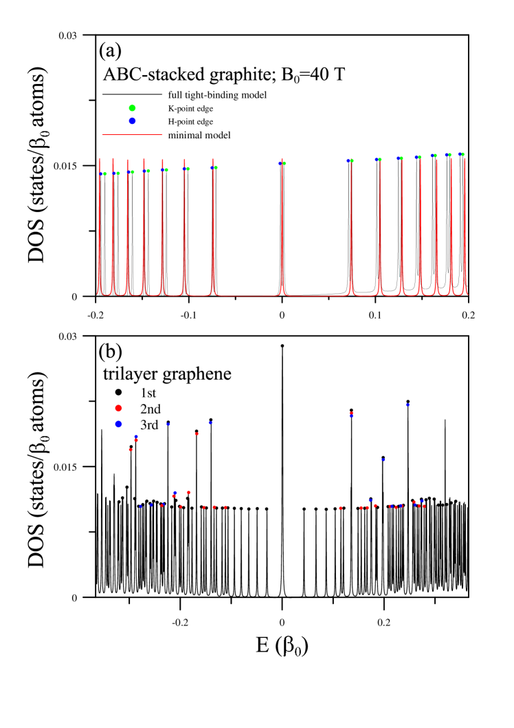
Figure 31: DOS of ABC-stacked (a) graphite and (b) trilayer graphene under $B_{0}=40$ T. The black and red curves in (a) represent the calculations from the tight-binding model and minimal model, respectively.

Figure 32: (a) Absorption spectra of rhombohedral graphite and (b) trilayer ABC-stacked graphene under $B_{0}=40$ T.

Figure 33: $B_{0}$-dependent absorption frequencies for the ABC-stacked (a) graphite and (b) graphene. In (b), the solid and dashed curves represent the intragroup and intergroup absorption frequencies, respectively.

Figure 35: Band structures of (a) (50,50), (b) (90,0), (c) (91,0) and (d) (80,20) carbon nanotubes at various magnetic-field and ${B_{0}=0}$ and 40 T. Also shown in (a) are that of (100,100) nanotube at ${\alpha\,=\pi\,/2}$ (orange curves), and in the insets of (b) and (d) are narrow energy gaps.

Figure 36: Magnetic-flux-dependent energy gaps for (a) (50,50), (b) (90,0), (c) (91,0) and (d) (65,35) carbon nanotubes at various magnetic-field directions.

Figure 37: Density of states for (a) (50,50), (b) (90,0), (c) (91,0) and (d) (65,35) carbon nanotubes at various magnetic-field directions.

Figure 38: The subenvelope functions of the (50,50) nanotube at ${k_{x}=2/3}$ for (a) ${J^{c}=50}$, (b) ${J^{c}=51}$ and (c) ${J^{c}=52}$. ${B_{0}=0}$ and ($B_{0}$=40 T,${\alpha\,=\pi\,/2}$) are, respectively, shown by the black and red curves. Also shown are those of the (100,100) nanotube for (d) ${J^{c}=100}$ and (e) ${J^{c}=101}$.

Figure 40: Optical absorption frequencies of (a) (50,50), and (b) (91,0) carbon nanotubes under various magnetic-field directions at $B_{0}$=40 T.

Figure 44: The subenvelope functions of a ${N_{y}=100}$ zigzag nanoribbon for (a) ${J^{c}=2}$, (b) ${J^{c}=1}$; (c) ${J^{v}=1}$, and those of a ${N_{y}=180}$ armchair system for (d) ${J^{c}=2}$, (e) ${J^{c}=1}$; (f) ${J^{v}=1}$.

Figure 45: The magnetic subenvelope functions of a ${N_{y}=100}$ zigzag nanoribbon at ${B_{0}=40}$ T and ${k_{x}=2/3}$ for (a)-(c) ${n^{c}=2-0}$ $\&$ (e)-(f) ${n^{v}=0-1}$. Also shown are those of ${n^{c}=1}$ at (f)-(j) various $k_{x}$s (triangles in Fig. 42(c)).

Figure 46: Optical absorption spectra of (a) ${N_{y}=100}$ zigzag and (b) ${N_{y}=180}$ armchair nanoribbons. Two subscripts in absorption peak frequency represents indexes of the initial valence and final conduction bands.

Figure 47: Magneto-optical absorption spectra for a ${N_{y}=100}$ zigzag nanoribbon at (a) ${B_{0}=40}$ T, (b) ${60}$ T $\&$ (c) 80 T and a ${N_{y}=180}$ armchair nanoribbon at (d) ${B_{0}}$=40 T. Also shown in (a) is that of monolayer graphene (red curve).

Figure 48: Magneto-absorption frequencies of the initial six prominent peaks for (a) ${N_{y}=100}$ zigzag and ${N_{y}=180}$ armchair graphene nanoribbons. The red dots are inter-LL optical excitation frequencies of monolayer graphene.

References

- [1] R. Robertson, J. J. Fox, and A. E. Martin, Two types of diamond, Proc. R. Soc. 1934, 232, 463-U85.
- [2] J. D. Bernal, The Structure of Graphite, Proc. R. Soc. London, Ser. A 1924, 106, 749.
- [3] H. Lipson, and A. R. Stokes, The Structure of Graphite, Proc. R. Sot. London, Ser. A 1942, 181, 101.
- [4] M. S. Dresselhaus, and G. Dresselhaus, Intercalation compounds of graphite, Adv. Phys. 1980, 30, 139-326.
- [5] K. S. Novoselov, A. K. Geim, S. V. Morozov, D. Jiang, Y. Zhang, S. V. Dubonos, I. V. Grigorieva, et al., Electric field effect in atomically thin carbon film, Science. 2004, 306, 666-9.
- [6] X. Li, X. Wang, L. Zhang, S. Lee, and H. Dai, Chemically derived, ultrasmooth graphene nanoribbon semiconductors, Science 2008, 319, 1229-32.
- [7] S. Iijima, Helical microtubules of graphitic carbon, Nature 1991, 354, 56-8.
- [8] J Liu, A. G. Rinzler, H.J. Dai, J. H. Hafner, R. K. Bradley, and P. J. Boul, et al., Fullerene pipes, Science 1998, 280, 1253-6.
- [9] Z. Q. Li, E. A. Henriksen, Z. Jiang, Z. Hao, M. C. Martin, P. Kim, et al., Band structure asymmetry of bilayer graphene revealed by infrared spectroscopy, Phys. Rev. Lett. 2009, 102, 037403.
- [10] J. C. Blancon, M. Paillet, H. N. Tran, X. T. Than, S. A. Guebrou, A. Ayari, et al., Direct measurement of the absolute absorption spectrum of individual semiconducting single-wall carbon nanotubes, Nat. Comm. 2013, 4, 2542.
- [11] D. M. Otpmebs, and H. F. Rase, Potassium grahites prepared by mixed-reaction technique, Carbon 1966, 4, 125-7.
- [12] N. Emery, C. Herold, J. F. Mareche, and P. Lagrange, Synthesis and superconducting properties of CaC6, Sci. Tech. Adv. Mater. 2008, 9, 044102.
- [13] M. S. Dresselhaus, and G. Dresselhaus, Intercalation compounds of graphite, Advances in Physics, 2002, 51, 1-186.
- [14] I. Belash, A. Bronnikov, O. Zharikov, A. Pal’nichenko, Superconductivity of graphite intercalation compound with lithium C2Li, Solid State Commun. 1989, 69, 921.
- [15] C. Lee, X. Wei, J. W. Kysar, and J. Hone, Measurement of the elastic properties and intrinsic strength of monolayer graphene, Science 2008, 321. 385-8.
- [16] A. H. Castro Neto, F. Guinea, N. M. R. Peres, K. S. Novoselov, and A. K. Geim, The electronic properties of graphene. Rev. Mod. Phys. 2009, 81. 109-62.
- [17] E. McCann, and M. Koshino, The electronic properties of bilayer graphene, Rep. Prog. Phys. 2013, 76, 056503.
- [18] Y. H. Ho, Y. H. Chiu, D. H. Lin, C. P. Chang, and M. F. Lin, Magneto-optical selection rules in bilayer Bernal graphene, ACS Nano 2010, 4, 1465-72.
- [19] D. S. L. Abergel, and V. I. Fal’ko, Optical and magneto-optical far-infrared properties of bilayer graphene, Phys. Rev. B 2007, 75, 155430.
- [20] M. Orlita, C. Faugeras, J. Borysiuk, J. M. Baranowski, W. Strupiski, M. Sprinkle, et al. Magneto-optics of bilayer inclusions in multilayered epitaxial graphene on the carbon face of SiC, Phys. Rev. B 2011, 83, 125302.
- [21] Z. Jiang, E. A. Henriksen, L. C. Tung, Y. J. Wang, M. E. Schwartz, M. Y. Han, et al. Infrared spectroscopy of Landau levels of graphene. Phys. Rev. Lett. 2007, 98, 197403.
- [22] P. Kuhne, V. Darakchieva, R. Yakimova, J. D. Tedesco, R. L. Myers-Ward, C. R. Eddy, et al. Polarization selection rules for inter-Landau-level transitions in epitaxial graphene revealed by the infrared optical Hall effect. Phys. Rev. Lett. 2013, 111, 077402.
- [23] M. Orlita, C. Faugeras, P. Plochocka, P. Neugebauer, G. Martinez, D. K. Maude, et al., Approaching the Dirac point in high-mobility multilayer epitaxial graphene, Phys. Rev. Lett. 2008, 101, 267601.
- [24] P. Plochocka, C. Faugeras, M. Orlita, M. L. Sadowski, G. Martinez, M. Potemski, et al., High-energy limit of massless Dirac fermions in multilayer graphene using magneto-optical transmission spectroscopy, Phys. Rev. Lett. 2008, 100, 087401.
- [25] T. N. Do, P. H. Shih, C. P. Chang, C. Y. Lin, and M. F. Lin, Rich magneto-absorption spectra of AAB-stacked trilayer graphene, Phys. Chem. Chem. Phys. 2016, 18, 17597.
- [26] C. Y. Lin, J. Y. Wu, Y. J. Ou, Y. H. Chiu, and M. F. Lin, Magneto-electronic properties of multilayer graphenes, Phys. Chem. Chem. Phys. 2015, 17, 26008-35.
- [27] Y. H. Lai, J. H. Ho, C. P. Chang, and M. F. Lin, Magnetoelectronic properties of bilayer Bernal graphene, Phys. Rev. B 2008, 77, 085426.
- [28] E. McCann, and V. I. Fal’ko, Landau-level degeneracy and quantum hall effect in a graphite bilayer, Phys. Rev. Lett. 2006, 96, 086805.
- [29] H. Min, and A. H. MacDonald, Chiral decomposition in the electronic structure of graphene multilayers, Phys. Rev. B 2008, 77, 155416.
- [30] S. H. R. Sena, J. M. Pereira, F. M. Peeters, and G. A. Faria, Landau levels in asymmetric graphene trilayers, Phys. Rev. B 2011, 84, 205448.
- [31] C. Y. Lin, J. Y. Wu, Y. H. Chiu, C. P. Chang, and M. F. Lin, Stacking-dependent magnetoelectronic properties in multilayer graphene, Phy. Rev. B 2014, 90, 205434.
- [32] Y. P. Lin, J. Wang, J. M. Lu, C. Y. Lin, and M. F. Lin, Energy spectra of ABC-stacked trilayer graphene in magnetic and electric fields, RSC Adv. 2014, 4, 56552-60.
- [33] N. T. T. Tran, S. Y. Lin, O. E. Glukhova, and M. F. Lin, Configuration-induced rich electronic properties of bilayer graphene, J Phys. Chem. C 2015, 119, 10623-30.
- [34] T. N. Do, C. Y. Lin, Y. P. Lin, P. H. Shih, and M. F. Lin, Configuration-enriched magnetoelectronic spectra of AAB-stacked trilayer graphene, Carbon 2015, 94, 619-32.
- [35] Y. K. Huang, S. C. Chen, Y. H. Ho, C. Y. Lin, and M. F. Lin, Feature-rich magnetic quantization in sliding bilayer graphenes, Sci. Rep. 2014, 4, 7509.
- [36] K. S. Novoselov, A. K. Geim, S. V. Morozov, D. Jiang, M. I. Katsnelson, I. V. Grigorieva, et al, Two-dimensional gas of massless Dirac fermions in graphene, Nature 2005, 438, 197-200.
- [37] Y. B. Zhang, Y. W. Tan, H. L. Stormer, and P. Kim, Experimental observation of the quantum Hall effect and Berry’s phase in graphene, Nature 2005, 438, 201-4.
- [38] K. S. Novoselov, E. McCann, S. V. Morozov, V. I. Fal’ko, M. I. Katsnelson, U. Zeitler, et al, Unconventional quantum Hall effect and Berry’s phase of 2 in bilayer graphene, Nat. Phys. 2006, 2, 177-80.
- [39] T. Taychatanapat, K. Watanabe, T. Taniguchi, and P. J. Herrero, Quantum Hall effect and Landau-level crossing of Dirac fermions in trilayer graphene, Nat. Phys. 2008, 7, 621-5.
- [40] L. Zhang, Y. Zhang, J. Camacho, M. Khodas, and I. Zaliznyak, The experimental observation of quantum Hall effect of chiral quasiparticles in trilayer graphene, Nat. Phys. 2011, 7, 953-7.
- [41] X. Xia, J, Wang, F. Zhang, Z. D. Hu, C. Liu, X. Yan, et al., Multi-mode plasmonically induced transparency in dual coupled graphene-integrated ring resonators, Plasmonics 2015, 10, 1409-15.
- [42] F. H. L. Koppens, D. E. Chang, and F. J. G. de Abajo, Graphene plasmonics: a platform for strong light-matter interactions, Nano Lett. 2011, 11, 3370-7.
- [43] J. Christensen, A. Manjavacas, S. Thongrattanasiri, F. H. L. Koppens, and F. J. G. de Abajo, Graphene plasmon waveguiding and hybridization in individual and paired nanoribbons, ACS Nano, 2012, 6, 431-40.
- [44] H. Yan, T. Low, W. Zhu, Y. Wu, M. Freitag, X. Li, et al., Damping pathways of mid-infrared plasmons in graphene nanostructures, Nat. Photon. 2013, 7, 394-9.
- [45] J. C. Charlier, X. Gonze, and J. P. Michenaud, First principles study of the stacking effect on the electronic properties of graphite, Carbon 1994, 32, 289.
- [46] J. K. Lee, S. C. Lee, J. P. Ahn, S. C. Kim, J. I. B. Wilson, and P. John, The growth of AA graphite on (111) graphite, J. Chem. Phys. 2008, 129, 234709.
- [47] S. Horiuchi, T. Gotou, M. Fujiwara, R. Sotoaka, M. Hirata, K. K. Kimoto et al., Carbon nanofilm with a new structure and property, Jpn. J. Appl. Phys. 2003, 47, 1073.
- [48] J. Borysiuk, J. Sotys, and J. Piechota, Stacking sequence dependence of graphene layers on SiC (000)-Experimental and theoretical investigation, J. Appl. Phys. 2011, 109, 093523.
- [49] K. S. Kim, A. L. Walter, L. Moreschini, T. Seyller, K. Horn, E. Rotenberg, et al.,. Coexisting massive and massless Dirac fermions in symmetry-broken bilayer graphene. Nat. Mater. 2013, 12, 887-92.
- [50] C. Bao, W. Yao, E. Wang, C. Chen, J. Avila, M. C. Asensio, and S. Zhou, Stacking-dependent electronic structure of trilayer graphene resolved by nanospot angle-resolved photoemission spectroscopy, Nano Lett. 2017, 8, 1564.
- [51] I. Lobato, and B. Partoens, Multiple Dirac particles in AA-stacked graphite and multilayers of graphene, Phys. Rev. B 2011, 83, 165429.
- [52] J. C. Charlier, J. VP. Michenaud, X. Gonze, and J. VP. Vigneron. Tight-binding model for the electronic properties of simple hexagonal graphite. Phys. Rev. B 1991, 44, 13237.
- [53] C. L. Lu, C. P. Chang, and M. F. Lin, Magneto-electronic properties of the AA- and ABC-stacked graphites, Eur. Phys. J. B 60, 161-9.
- [54] R. B. Chen, and Y. H. Chiu, Landau subband and Landau level properties of AA-stacked graphene superlattice, J Nanosci. Nanotechnol. 2012, 12, 2557-66.
- [55] Y. H. Ho, J. Y. Wu, R. B. Chen, Y. H. Chiu, and M. F. Lin, Optical transitions between Landau levels: AA-stacked bilayer graphene, Appl. Phys. Lett. 2010, 97, 101905.
- [56] R. B. Chen, Y. H. Chiu, and M. F. Lin, A theoretical evaluation of the magneto-optical properties of AA-stacked graphite, Carbon 2012, 54, 248.
- [57] R. B. Chen, Y. H. Chiu, and M. F. Lin, Beating oscillations of magneto-optical spectra in simple hexagonal graphite, Comput. Phys. Commun. 2014, 189, 60.
- [58] J. H. Ho, C. L. Lu, C. C. Hwang, C. P. Chang, and M. F. Lin, Coulomb excitations in AA- and AB-stacked bilayer graphites, Phys. Rev. B 2006, 74, 085406.
- [59] J. Y. Wu, Godfrey Gumbs, and M. F. Lin, Combined effect of stacking and magnetic field on plasmon excitations in bilayer graphene, Phys. Rev. B 2014, 89, 165407.
- [60] Y. C. Chuang, J. Y. Wu, and M. F. Lin, Electric-field-induced plasmon in AA-stacked bilayer graphene, Annals of Physics 2013, 339, 298.
- [61] R. B. Chen, C. W. Chiu, and M. F. Lin, Magnetoplasmons in simple hexagonal graphite, RSC Adv. 2015, 5, 53736-40.
- [62] C. W. Chiu, F. L. Shyu, M. F. Lin, G. Gumbs, and O. Roslyak, Anisotropy of k-plasmon dispersion relation of AA-stacked graphite, J. Phys. Soc. Jpn. 2012, 81, 104703.
- [63] Y. F. Hsu, and G. Y. Guo, Anomalous integer quantum Hall effect in AA-stacked bilayer graphene, Phys. Rev. B 2010, 82, 165404.
- [64] A. I. Cocemasov, D. L. Nika, and A. A. Balandin, Phonons in twisted bilayer graphene, Phys. Rev. B 2013, 88, 035428.
- [65] Z. Sun, A. R. O. Raji, Y. Zhu, C. Xiang, Z. Yan, C. Kittrell, et al., Large-area Bernal-stacked bi-, tri-, and tetralayer graphene, ACS Nano, 2012, 6, 9790-6.
- [66] P. Lauffer, K. Emtsev, R. Graupner, T. Seyller, L. Ley, S. Reshanov, and H. Weber, Atomic and electronic structure of few-layer graphene on SiC (0001) studied with scanning tunneling microscopy and spectroscopy, Phys. Rev. B 2008, 77, 155426.
- [67] D. Pierucci, T. Brumme, J. C. Girard, M. Calandra, M. G. Silly, F. Sirotti, et al., Atomic and electronic structure of trilayer graphene/SiC(0001): Evidence of strong dependence on stacking sequence and charge transfer, Sci. Rep. 2016, 6, 33487.
- [68] A. Gruneis, C. Attaccalite, T. Pichler, V. Zabolotnyy, H. Shiozawa, S. L. Molodtsov, et al., Electron-electron correlation in graphite: a combined angle-resolved photoemission and first-principles study, Phys. Rev. Lett. 2008, 100, 037601.
- [69] C. Coletti, S. Forti, A. Principi, K. V. Emtsev, A. A. Zakharov, K. M. Daniels, et al., Revealing the electronic band structure of trilayer graphene on SiC: An angle-resolved photoemission study, Phys. Rev. B 2013, 88, 155439.
- [70] T. Ohta, A. Bostwick, J. L. McChesney, T. Seyller, K. Horn, and E. Rotenberg, Interlayer interaction and electronic screening in multilayer graphene investigated with angle-resolved photoemission spectroscopy, Phys. Rev. Lett. 2007, 98, 206802.
- [71] T. Ohta, A. Bostwick, T. Seyller, K. Horn, and E. Rotenberg, Controlling the electronic structure of bilayer graphene, Science 2006, 313, 951.
- [72] Z. Klusek, Investigations of splitting of the bands in graphite by scanning tunneling spectroscopy, Appl. Surf. Sci. 1999, 151, 251.
- [73] G. Li, A. Luican, and E. Y. Andrei, Scanning tunneling spectroscopy of graphene on graphite, Phys. Rev. Lett. 2009, 102, 176804.
- [74] G. Li, and E. Y. Andrei, Observation of Landau levels of Dirac fermions in graphite, Nat. Phys. 2007, 3, 623-7.
- [75] T. Matsui, H. Kambara, Y. Niimi, K. Tagami, M. Tsukada, and H. Fukuyama, STS observations of Landau levels at graphite surfaces, Phys. Rev. Lett. 2005, 94, 226403.
- [76] D. L. Miller, K. D. Kubista, G. M. Rutter, M. Ruan, W. A. de Heer, P. N. First, et al., Observing the quantization of zero mass carriers in graphene, Science 2009, 324, 924-7.
- [77] L. J. Yin, S. Y. Li, J. B. Qiao, J. C. Nie, and L. He, Landau quantization in graphene monolayer, Bernal bilayer, and Bernal trilayer on graphite surface, Phys. Rev. B 2015, 91, 115405.
- [78] E. A. Taft, and H. R. Philipp, Optical properties of graphite, Phys. Rev. 1965, 138, A197.
- [79] K. F. Mak, J. Shan, and T. F. Heinz, Seeing many-body effects in single- and few-layer graphene: Observation of two-dimensional saddle-point excitons, Phys. Rev. Lett. 2011, 106, 046401.
- [80] V. G. Kravets, A. N. Grigorenko, R. R. Nair, P. Blake, S. Anissimova, K. S. Novoselov, et al., Spectroscopic ellipsometry of graphene and an exciton-shifted van Hove peak in absorption, Phys. Rev. B 2010, 81, 155413.
- [81] Y. H. Ho, Y. H. Chiu, W. P. Su, and M. F. Lin, Magneto-absorption spectra of Bernal graphite, Appl. Phys. Lett. 2011, 99, 011914.
- [82] K.-C. Chuang, A. M. R. Baker, and R. J. Nicholas, Magnetoabsorption study of Landau levels in graphite, Phys. Rev. B 2009, 80, 161410(R).
- [83] M. Orlita, C. Faugeras, J. M. Schneider, G. Martinez, D. K. Maude, and M. Potemski, Graphite from the viewpoint of Landau level spectroscopy: an effective graphene bilayer and monolayer, Phys. Rev. Lett. 2009, 102, 166401.
- [84] N. A. Goncharuk, L. Ndvornik, C. Faugeras, M. Orlita, and L. Smrka, Infrared magnetospectroscopy of graphite in tilted fields, Phys. Rev. B 2012, 86, 155409.
- [85] M. Orlita, C. Faugeras, A.-L. Barra, G. Martinez, M. Potemski, D. M. Basko, et al., Infrared magneto-spectroscopy of two-dimensional and three-dimensional massless fermions: A comparison, J. App. Phys. 2015, 117, 112803.
- [86] M. Orlita, C. Faugeras, G. Martinez, D. K. Maude, M. L. Sadowski, and M. Potemski, Dirac fermions at the H Point of graphite: magnetotransmission studies. Phys. Rev. Lett. 2008, 100, 136403.
- [87] W. W. Toyt, and M. S. Dresselhaus, Minority carriers in graphite and the H-point magnetoreflection spectra, Phys. Rev. B 1977, 15, 4077.
- [88] Z. Q. Li, S.-W. Tsai, W. J. Padilla, S. V. Dordevic, K. S. Burch, Y. J. Wang, et al., Infrared probe of the anomalous magnetotransport of highly oriented pyrolytic graphite in the extreme quantum limit, Phys. Rev. B 2006, 74, 195404.
- [89] P. R. Wallace, The band theory of graphite, Phys. Rev. 1947, 71, 622.
- [90] J. C. Slonczewski, and P. R. Weiss, Band structure of graphite, Phys. Rev. 1958, 109, 272.
- [91] J. W. McClure, Theory of diamagnetism of graphite, Phys. Rev. 1960, 119, 606.
- [92] Y. H. Ho, J. Wang, Y. H. Chiu, M. F. Lin, and W. P. Su, Characterization of Landau subbands in graphite: A tight-binding study, Phys. Rev. B 2011, 83, 121201.
- [93] K. Nakao, Landau level structure and magnetic breakthrough in graphite, J. Phys. Soc. Jpn. 1976, 40, 761-8.
- [94] M. Inoue, Landau levels and cyclotron resonance in graphite, J. Phys. Soc. Jpn. 1962, 17, 808-19.
- [95] Q. Y. Lin, T. Q. Li, Z. J. Liu, Y. Song, L. L. He, Z. J. Hu, et al., High-resolution TEM observations of isolated rhombohedral crystallites in graphite blocks, Carbon 2012, 50, 2369.
- [96] Z. Zhou, W. G. Bouwman, H. Schut, and C. Pappas, Interpretation of X-ray diffraction patterns of (nuclear) graphite, Carbon 2014, 69, 17.
- [97] N. S. Saenko, The X-ray diffraction study of three-dimensional disordered network of nanographites: Experiment and theory, Physics Procedia 2012, 23, 102.
- [98] Y. Hishiyama, and M. Nakamura, X-ray diffraction in oriented carbon films with turbostratic structure, Carbon 1995, 33, 1399.
- [99] P. Xu, Y. R. Yang, S. D. Barber, J. K. Schoelz, D. Qi, M. L. Ackerman, et al., New scanning tunneling microscopy technique enables systematic study of the unique electronic transition from graphite to graphene, Carbon 2012, 50, 4633.
- [100] C. D. Zeinalipour-Yazdi, and D. P. Pullman, A new interpretation of the scanning tunneling microscope image of graphite, Chem. Phys. 2008, 348, 233.
- [101] B. A. Bernevig, T. L. Hughes, S. Raghu, and D. P. Arovas, Theory of the three-dimensional quantum hall effect in graphite, Phys. Rev. Lett. 2007, 99, 146804.
- [102] J. Hass, W. A. De Heer, and E. H. Conrad, The growth and morphology of epitaxial multilayer graphene, J. Phys.: Condens. Matter 2008, 20, 323202.
- [103] J. Coraux, A. T. N Diaye, C. Busse, and T. Michely, Structural coherency of graphene on Ir (111), Nano Lett. 2008, 8, 565.
- [104] A. Ismach, C. Druzgalski, S. Penwell, A. Schwartzberg, M. Zheng, A. Javey, J. Bokor, and Y. Zhang, Direct chemical vapor deposition of graphene on dielectric surfaces, Nano Lett. 2010, 10, 1542.
- [105] H. J. Park, J. Meyer, S. Roth, and V. Skkalov, Growth and properties of few-layer graphene prepared by chemical vapor deposition, Carbon 2010, 48, 1088.
- [106] A. Reina, X. Jia, J. Ho, D. Nezich, H. Son, V. Bulovic, M. S. Dresselhaus, and J. Kong, Large area, few-layer graphene films on arbitrary substrates by chemical vapor deposition, Nano Lett. 2008, 9, 30.
- [107] S. J. Chae, F. Gune, K. K. Kim, E. S. Kim, G. H. Han, S. M. Kim, et al, Synthesis of large-area graphene layers on poly-nickel substrate by chemical vapor deposition: wrinkle formation, Adv. Mater. 2009, 21, 2328.
- [108] G. Zhao, J. Li, X. Ren, C. Chen, and X. Wang, Few-layered graphene oxide nanosheets as superior sorbents for heavy metal ion pollution management, Environ. Sci. Technol. 2011, 45, 10454.
- [109] S. Stankovich, D. A. Dikin, R. D. Piner, K. A. Kohlhaas, A. Kleinhammes, Y. Jia, et al., Synthesis of graphene-based nanosheets via chemical reduction of exfoliated graphite oxide, Carbon 2007, 45, 1558.
- [110] C. Rao, K. Subrahmanyam, H. R. Matte, B. Abdulhakeem, A. Govindaraj, B. Das, P. Kumar, A. Ghosh, and D. J. Late, A study of the synthetic methods and properties of graphenes, Sci. Technol. Adv. Mater. 2010, 11, 054502.
- [111] B. Qin, T. Zhang, H. Chen, and Y. Ma, The growth mechanism of few-layer graphene in the arc discharge process, Carbon 2016, 102, 494.
- [112] Z. S. Wu, W. Ren, L. Gao, B. Liu, C. Jiang, and H. M, Synthesis of high-quality graphene with a pre-determined number of layers, Carbon 2009, 47, 4939.
- [113] Y. Wu, B. Wang, Y. Ma, Y. Huang, N. Li, F. Zhang, et al., Efficient and largescale synthesis of few-layered graphene using an arc-discharge method and conductivity studies of the resulting films, Nano Research 2010, 3, 661.
- [114] Z. Li, H. Zhu, D. Xie, K. Wang, A. Cao, J. Wei, et al., Flame synthesis of few-layered graphene/graphite films, Chem. Commun. 2011, 47, 3520.
- [115] P. Xu, Y. Yang, D. Qi, S. Barber, J. Schoelz, M. Ackerman, et al., Electronic transition from graphite to graphene via controlled movement of the top layer with scanning tunneling microscopy, Phys. Rev. B 2012, 86, 085428.
- [116] Y. Que, W. Xiao, H. Chen, D. Wang, S. Du, and H. -J. Gao, Stacking-dependent electronic property of trilayer graphene epitaxially grown on Ru (0001), Appl. Phys. Lett. 2015, 107, 263101.
- [117] R. Xu, L. J. Yin, J. B. Qiao, K. K. Bai, J. C. Nie, and L. He, Direct probing of the stacking order and electronic spectrum of rhombohedral trilayer graphene with scanning tunneling microscopy, Phys. Rev. B 2015, 91, 035410.
- [118] D. Pierucci, H. Sediri, M. Hajlaoui, J. C. Girard, T. Brumme, M. Calandra, et al, Evidence for flat bands near the Fermi level in epitaxial rhombohedral multilayer graphene, ACS Nano 2015, 9, 5432.
- [119] R. R. Haering, Babd structure of rhombohedral graphite, Can. J. Phys. 1958, 36, 352.
- [120] J. W. McClure, Electron energy band structure and electronic properties of rhombohedral graphite, Carbon 1969, 7, 425.
- [121] N. Luiggi, and M. Gmez, Rhombohedral graphite: Comparative study of the electronic properties, J Mol. Struc. THEOCHEM 2009, 897, 118-28.
- [122] H. Kempa, P. Esquinazi, and Y. Kopelevich, Integer quantum Hall effect in graphite, Solid State Commun. 2006, 138, 118-22.
- [123] C. H. Ho, C. P. Chang, and M. F. Lin, Landau subband wave functions and chirality manifestation in rhombohedral graphite, Solid State Commun. 2014, 197, 11.
- [124] C. H. Ho, C. P. Chang, W. P. Su, and M. F. Lin, Precessing anisotropic Dirac cone and Landau subbands along a nodal spiral, New J. Phys. 2013, 15, 053032.
- [125] D. P. Arovas, and F. Guinea, Stacking faults, bound states, and quantum Hall plateaus in crystalline graphite, Phys. Rev. B 2008, 78, 245416.
- [126] C. W. Chiu, Y. C. Huang, F. L. Shyu, and M. F. Lin, Excitation spectra of ABC-stacked graphene superlattice, Appl. Phys. Lett. 2011, 98, 261920.
- [127] C. W. Chiu, Y. C. Huang, S. C. Chen, M. F. Lin, and F. L. Shyu, Low-frequency electronic and optical properties of rhombohedral graphite, Phys. Chem. Chem. Phys. 2011, 13, 6036-42.
- [128] Y. P. Lin, C. Y. Lin, Y. H. Ho, T.N. Do and M. F. Lin, Magneto-optical properties of ABC-stacked trilayer graphene, Phys. Chem. Chem. Phys. 2015, 17, 15921.
- [129] C. H. Ho, C. P. Chang, and M. F. Lin, Optical magnetoplasmons in rhombohedral graphite with a three-dimensional Dirac cone structure, J. Phys. Condens. Matter 2015, 27, 125602.
- [130] R. Saito, M. Fujita, G. Dresselhaus, and M. S. Dresselhaus, Electronic structure of graphene tubules based on C60, Phys. Rev. B 1992, 46, 1804.
- [131] C. L. Kane, and E. J. Mele, Size, shape, and low energy electronic structure of carbon nanotubes, Phys. Rev. Lett 1997, 78, 1932.
- [132] M. Ouyang, J. L. Huang, C. L. Cheung, and C. M. Lieber, Energy gaps in metallic single-walled carbon nanotubes, Science 2001, 292, 702.
- [133] P. Ruffieux, J. Cai, N. C. Plumb, L. Patthey, D. Prezzi, A. Ferretti, and R. Fasel, Electronic structure of atomically precise graphene nanoribbons, ACS Nano 2012, 6, 6930-5.
- [134] Y. Sugiyama, O. Kubo, R. Omura, M. Shigehara, H. Tabata, N. Mori, et al., Spectroscopic study of graphene nanoribbons formed by crystallographic etching of highly oriented pyrolytic graphite, Appl. Phys. Lett. 2014, 105, 123116.
- [135] H. Huang, D. Wei, J. Sun, S. L. Wong, Y. P. Feng, A. C. Neto, and A. T. S. Wee, Spatially resolved electronic structures of atomically precise armchair graphene nanoribbons, Sci. Rep. 2012, 2, 983.
- [136] H. Söde, L. Talirz, O. Gröning, C. A. Pignedoli, R. Berger, X. Feng, and P. Ruffieux, Electronic band dispersion of graphene nanoribbons via Fourier-transformed scanning tunneling spectroscopy, Phys. Rev. B 2015, 91, 045429.
- [137] Y. C. Chen, D. G. De Oteyza, Z. Pedramrazi, C. Chen, F. R. Fischer, and M. F. Crommie, Tuning the band gap of graphene nanoribbons synthesized from molecular precursors, ACS Nano 2013, 7, 6123-8.
- [138] H. C. Chung, M. H. Lee, C. P. Chang, and M. F. Lin, Exploration of edge-dependent optical selection rules for graphene nanoribbons, Opt. Express, 2011, 19, 23350.
- [139] V. A. Saroka, M. V. Shuba, and M. E. Portnoi, Optical selection rules of zigzag graphene nanoribbons, Phys. Rev. B 2017, 95, 155438.
- [140] K. I. Sasaki, K. Kato, Y. Tokura, K. Oguri, and T. Sogawa, Theory of optical transitions in graphene nanoribbons, Phys. Rev. B 2011, 84, 085458.
- [141] M. F. Lin, and K. W. -K. Shung, Magnetoconductance of carbon nanotubes, Phys. Rev. B 1995, 51, 7592.
- [142] H. Ajiki, and T. J. Ando, Magnetic properties of carbon nanotubes, J. Phys. Soc. Jap 1993, 62, 2470-80.
- [143] F. L. Shyu, C. P. Chang, R. B. Chen, C. W. Chiu, and M. F. Lin, Magnetoelectronic and optical properties of carbon nanotubes, Phys. Rev. B 2003, 67, 045405.
- [144] S. Roche, G. Dresselhaus, M. S. Dresselhaus, and R. Saito, Aharonov-Bohm spectral features and coherence lengths in carbon nanotubes, Phys. Rev. B 2000, 62, 16092.
- [145] S. Zaric, G. N. Ostojic, J. Kono, J. Shaver, V. C. Moore, M. S. Strano, et al., Optical signatures of the Aharonov-Bohm phase in single-walled carbon nanotubes, Science 2004, 304, 1129.
- [146] N. Akima, Y. Iwasa, S. Brown, A. M. Barbour, J. B. Cao, J. L. Musfeldt, et al., Strong anisotropy in the far-infrared absorption spectra of stretch-aligned single-walled carbon nanotubes, Adv. Mater. 2006, 18, 1166.
- [147] C. Jien, W. Qian, and D. Hongjie, Electron transport in very clean, as-grown suspended carbon nanotubes, Nat. Mater. 2005, 4, 745-9.
- [148] C. Jien, W. Qian, R. Marco, and D. Hongjie, Aharonov-Bohm interference and beating in single-walled carbon-nanotube interferometers, Phys. Rev. Lett. 2004, 93, 216803.
- [149] A. Bachtold, C. Strunk, J. P. Salvetat, J. M. Bonard, L. Forro, T. Nussbaumer, and C. Schonenberger, Aharonov-Bohm oscillations in carbon nanotubes, Nature 1998, 397, 673-5.
- [150] H. Ajiki, and T. Ando, Energy bands of carbon nanotubes in magnetic fields, J Phys. Soc. Jpn. 1996, 65, 505.
- [151] J. W. Bai, X. F. Duan, and Y. Huang, Rational fabrication of graphene nanoribbons using a nanowire etch mask, Nano Lett. 2009, 9, 2083-7.
- [152] L. C. Campos, V. R. Manfrinato, J. D. Sanchez-Yamagishi, J. Kong, and P. Jarillo-Herrero, Anisotropic etching and nanoribbon formation in single-layer graphene, Nano Lett. 2009, 9, 2600-4.
- [153] A. G. Cano-Marquez, F. J. Rodriguez-Macias, J. Campos-Delgado, C. G. Espinosa-Gonzalez, F. Tristan-Lopez, D. Ramirez-Gonzalez, et. al., Graphene sheets and ribbons produced by lithium intercalation and exfoliation of carbon nanotubes, Nano Lett. 2009, 9, 1527-33.
- [154] F. Cataldo, G. Compagnini, G. Patane, O. Ursini, G. Angelini, P. R. Ribic, et. al., Graphene nanoribbons produced by the oxidative unzipping of single-wall carbon nanotubes, Carbon 2010, 48, 2596-602.
- [155] D. V. Kosynkin, A. L. Higginbotham, A. Sinitskii, J. R. Lomeda, A. Dimiev, B. K. Price, et al., Longitudinal unzipping of carbon nanotubes to form graphene nanoribbons, Nature 2009, 458, 872-6.
- [156] Y. Z. Tan, B. Yang, K. Parvez, A. Narita, S. Osella, D. Beljonne, et al., Atomically precise edge chlorination of nanographenes and its application in graphene nanoribbons, Nat. Comm. 2013, 4, 2646.
- [157] J. M. Cai, P. Ruffieux, R. Jaafar, M. Bieri, T. Braun, S. Blankenburg, et al., Atomically precise bottom-up fabrication of graphene nanoribbons, Nature, 2010, 466, 470-3.
- [158] J. Campos-Delgado, J. M. Romo-Herrera, X. T. Jia, D. A. Cullen, H. Muramatsu, Y. A. Kim, et al., Bulk production of a new form of sp2 carbon: Crystalline graphene nanoribbons, Nano Lett. 2008, 8, 2773-8.
- [159] N. M. R. Peres, A. H. Castro Neto, and F. Guinea, Dirac fermion confinement in graphene, Phys Rev B 2006, 73, 241403-7(R).
- [160] Y. C. Huang, C. P. Chang, and M. F. Lin, Magnetic and quantum confinement effects on electronic and optical properties of graphene ribbons, Nanotechnology 2007, 18, 495401-9.
- [161] Y. C. Huang, M. F. Lin, and C. P. Chang, Landau levels and magnetooptical properties of graphene ribbons, J Appl Phys 2008, 103, 073709-16.
- [162] K. F. Mak, J. Shan, and T. F. Heinz, Electronic structure of few-layer graphene: Experimental demonstration of strong dependence on stacking sequence, Phys. Rev. Lett 2010, 104, 176404.
- [163] Y. C. Ou, J. K. Sheu, Y. H. Chiu, R. B. Chen, and M. F. Lin, Influence of modulated fields on the Landau level properties of graphene, Phys. Rev. B 2011, 83, 195405.
- [164] Y. H. Chiu, Y. C. Ou, Y. Y. Liao, M. F. Lin, Optical-absorption spectra of single-layer graphene in a periodic magnetic field, J. Vac. Sci. Technol. B 2010, 28, 386-90.
- [165] Y. C. Ou, Y. H. Chiu, P. H. Yang, and M. F. Lin, The selection rule of graphene in a composite magnetic field, Optics Express 2014, 22, 7473-91.
- [166] J. Y. Wu, S. C. Chen, G. Gumbs, and M. F. Lin, Feature-rich electronic excitations in external fields of 2D silicene, Phys. Rev. B 2016, 94, 205427.
- [167] J. Y. Wu, S. C. Chen, and M. F. Lin, Temperature-dependent Coulomb excitations in silicene, New J. Phys. 2014, 16, 125002.
- [168] J. Y. Wu, C. Y. Lin, G. Gumbs, and M. F. Lin, The effect of perpendicular electric field on temperature-induced plasmon excitations for intrinsic silicene, RSC Adv. 2015, 5, 51912-8.
- [169] P. H. Shih, Y. H. Chiu, J. Y. Wu, F. L. Shyu, and M. F. Lin, Coulomb excitations of monolayer germanene, Sci. Rep. 2017, 7, 40600.
- [170] S. C. Chen, C. L. Wu, J. Y. Wu, and M. F. Lin, Magnetic quantization of sp3 bonding in monolayer gray tin, Phys. Rev. B 2016, 94, 045410.
- [171] C. P. Chang, Exact solution of the spectrum and magneto-optics of multilayer hexagonal graphene, J. Appl. Phys. 2011, 110, 013725.
- [172] C. W. Chiu, S. H. Lee, S. C. Chen, and M. F. Lin, Absorption spectra of AA-stacked graphite, New J. Phys. 2010, 12, 083060.
- [173] K. Sugawara, T. Sato, S. Souma, T. Takahashi, and H. Suematsu, Fermi surface and edge-localized states in graphite studied by high-resolution angle-resolved photoemission spectroscopy, Phys. Rev. B 2006, 73, 045124.
- [174] D. A. Siegel, W. Regan, A. V. Fedorov, A. Zettl, and A. Lanzara, Charge-carrier screening in single-layer graphene, Phys. Rev. Lett. 2013, 110, 146802.
- [175] A. Bostwick, T. Ohta, T. Seyller, K. Horn, and E. Rotenberg, Quasiparticle dynamics in graphene, Nat. Phys. 2007, 3, 36-40.
- [176] T. Ohta, A. Bostwick, J. L. McChesney, T. Seyller, K. Horn, and E. Rotenberg, Interlayer interaction and electronic screening in multilayer graphene investigated with angle-resolved photoemission spectroscopy, Phys. Rev. Lett. 2007, 98, 206802.
- [177] T. Ohta, A. Bostwick, T. Seyller, K. Horn, and E. Rotenberg, Controlling the electronic structure of bilayer graphene, Science 2006, 313, 951-4.
- [178] A. Grneis, C. Attaccalite, T. Pichler, V. Zabolotnyy, H. Shiozawa, S. L. Molodtsov, et al., Electron-electron correlation in graphite: a combined angle-resolved photoemission and first-principles study, Phys. Rev. Lett. 2008, 100, 037601.
- [179] C. M. Cheng, C. J. Hsu, J. L. Peng, C. H. Chen, J. Y. Yuh, and K. D. Tsuei, Tight-binding parameters of graphite determined with angle-resolved photoemission spectra, Appl. Surf. Sci. 2015, 354, 229 V34.
- [180] R. Kundu, P. Mishra, B.R. Sekhar, M. Maniraj, and S.R. Barman, Electronic structure of single crystal and highly oriented pyrolytic graphite from ARPES and KRIPES, Physica B 2012, 407, 827-32.
- [181] C. S. Leem, Chul Kim, S. R. Park, M. K. Kim, H. J. Choi, and C. Kim, High-resolution angle-resolved photoemission studies of quasiparticle dynamics in graphite, Phys. Rev. B 2009, 79, 125438.
- [182] S. Y. Zhou, G.-H. Gweon, J. Graf, A. V. Fedorov, C. D. Spataru, R. D. Diehl, et. al., First direct observation of Dirac fermions in graphite, Nat. Phys. 2006, 2, 595-9.
- [183] Luican A, Li G, Reina A, Kong J, Nair R, Novoselov KS, et al., Single-layer behavior and its breakdown in twisted graphene layers, Phys. Rev. Lett. 2011, 106, 126802.
- [184] G. Li, A. Luican, J. L. Dos Santos, A. C. Neto, A. Reina, J. Kong, et al., Observation of Van Hove singularities in twisted graphene layers, Nat. Phys. 2010, 6, 109-13.
- [185] V. Cherkez, G. T. de Laissardiere, P. Mallet, and J.-Y. Veuillen, Van Hove singularities in doped twisted graphene bilayers studied by scanning tunneling spectroscopy, Phys. Rev. B 2015, 91, 155428.
- [186] M. Yankowitz, F. Wang, C. N. Lau, and B. J. LeRoy, Local spectroscopy of the electrically tunable band gap in trilayer graphene, Phys. Rev. B 2013, 87, 165102.
- [187] Y. Que, W. Xiao, H. Chen, D. Wang, S. Du, and H. J. Gao, Stacking-dependent electronic property of trilayer graphene epitaxially grown on Ru (0001), Appl. Phys. Lett. 2015, 107, 263101.
- [188] Z. Klusek, Investigations of splitting of the bands in graphite by scanning tunneling spectroscopy, Appl. Surf. Sci. 1999, 151, 251-61.
- [189] G. Li, A. Luican, and E. Y. Andrei, Scanning tunneling spectroscopy of graphene on graphite, Phys. Rev. Lett. 2009, 102, 176804.
- [190] J. S. Alden, A. W. Tsen, P. Y. Huang, R. Hovden, L. Brown, J. Park, et al., Strain solitons and topological defects in bilayer graphene, Proc. Natl. Acad. Sci. 2013, 110, 11256-60.
- [191] F. Guinea, M. Katsnelson, and M. Vozmediano, Midgap states and charge inhomogeneities in corrugated graphene, Phys. Rev. B 2008, 77, 075422.
- [192] F. Guinea, B. Horovitz, and P. Le Doussal, Gauge field induced by ripples in graphene, Phys. Rev. B 2008, 77, 205421.
- [193] J. W. G. Wilder, L. C. Venema, A. G. Rinzler, R. E. Smalley, and C. Dekker, Electronic structure of atomically resolved carbon nanotubes, Nature 1998, 391, 59-62.
- [194] T. W. Odom, J.-L. Huang, P. Kim, and C. M. Lieber, Atomic structure and electronic properties of single-walled carbon nanotubes, Nature 1998, 391, 62-4.
- [195] C. W. Chiu, S. C. Chen, Y. C. Huang, F. L. Shyu, and M. F. Lin, Critical optical properties of AA-stacked multilayer graphenes, Appl. Phys. Lett. 2013, 103, 041907.
- [196] A. Narita, X. Feng, Y. Hernandez, S. A. Jensen, M. Bonn, H. Yang, et al., Synthesis of structurally well-defined and liquid-phase-processable graphene nanoribbons, Nat. Chem. 2014, 6, 126-32.
- [197] L. Degiorgi, E. J. Nicol, O. Klein, G. Gruner, P. Wachter, S.-M. Huang, et al., Optical properties of the alkali-metal-doped superconducting fullerenes: K3C60 and Rb3C60, Phys. Rev. B 1994, 49, 7012.
- [198] K. Harigaya, and S. Abe, Optical-absorption spectra in fullerenes C60 and C70: Effects of Coulomb interactions, lattice fluctuations, and anisotropy, Phys. Rev. B 1994, 49, 16746.
- [199] I. A. Luk’yanchuk, and Y. Kopelevich, Phase analysis of quantum oscillations in graphite, Phys. Rev. Lett. 2004, 93, 166402.
- [200] N. Ubrig, P. Plochocka, P. Kossacki, M. Orlita, D. K. Maude, O. Portugall, and G. L. J. A. Rikken, High-field magnetotransmission investigation of natural graphite, Phys. Rev. B 2011, 83, 073401.
- [201] P. A. Obraztsov, G. M. Mikheev, S. V. Garnov, A. N. Obraztsov, and Y. P. Svirko, Polarization-sensitive photoresponse of nanographite, Appl. Phys. Lett. 2011, 98, 091903.
- [202] J. M. Zhang, and P. C. Eklun, Optical transmission of graphite and potassium graphite intercalation compounds, J Mater. Res. 1987, 2, 858-63.
- [203] E. Jung, S. Lee, S. Roh, X. Meng, S. Tongay, J. Kang, et al., Optical properties of NbCl5 and ZnMg intercalated graphite compounds, J. Phys. D: Appl. Phys. 2014, 47, 485304.
- [204] D. S. Kim, H. Kwon, A. Y. Nikitin, S. Ahn, L. Martin-Moreno, F. J. Garcia-Vidal, et al., Stacking Structures of Few-Layer Graphene Revealed by Phase-Sensitive Infrared Nanoscopy, ACS Nano. 2015, 9, 6765-73.
- [205] M. Koshino, and E. McCann, Landau level spectra and the quantum Hall effect of multilayer graphene, Phys. Rev. B 2011, 83, 165443.
- [206] L.-C. Tung, P. Cadden-Zimansky, J. Qi, Z. Jiang, and D. Smirnov, Measurement of graphite tight-binding parameters using high-field magnetoreflectance, Phys. Rev. B 2011, 84, 153405.
- [207] P. Kossacki, C. Faugeras, M. Kuhne, M. Orlita, A. A. L. Nicolet, J. M. Schneider, Electronic excitations and electron-phonon coupling in bulk graphite through Raman scattering in high magnetic fields, Phys. Rev. B 2011, 84, 235138.
- [208] Y. Kim, Y. Ma, A. Imambekov, N. G. Kalugin, A. Lombardo, A. C. Ferrari, et al., Magnetophonon resonance in graphite: High-field Raman measurements and electron-phonon coupling contributions, Phys. Rev. B 2012, 85, 121403(R).
- [209] P. Plochocka, P. Y. Solane, R. J. Nicholas, J. M. Schneider, B. A. Piot, D. K. Maude, O. Portugall, and G. L. J. A. Rikken, Origin of electron-hole asymmetry in graphite and graphene, Phys. Rev. B 2012, 85, 245410.
- [210] R. J. Nicholas, P. Y. Solane, and O. Portugall, Ultrahigh Magnetic Field Study of Layer Split Bands in Graphite, Phys. Rev. Lett. 2013, 111, 096802.
- [211] E. A. Henriksen, Z. Jiang, L. -C. Tung, M. E. Schwartz, M. Takita, Y. -J. Wang, et al., Cyclotron resonance in bilayer graphene, Phys. Rev. Lett. 2008, 100, 087403.
- [212] J. M. Pereira Jr., F. M. Peeters, and P. Vasilopoulos, Landau levels and oscillator strength in a biased bilayer of graphene, Phys. Rev. B 2007, 76, 115419.
- [213] A. B. Kuzmenko, E. van Heumen, D. van der Marel, P. Lerch, P. Blake, K. S. Novoselov, et al., Infrared spectroscopy of electronic bands in bilayer graphene, Phys. Rev. B 2009, 79, 115441.
- [214] L. M. Zhang, Z. Q. Li, D. N. Basov, and M. M. Fogler, Determination of the electronic structure of bilayer graphene from infrared spectroscopy, Phys. Rev. B 2008, 78, 235408.
- [215] M. L. Sadowski, G. Martinez, M. Potemski, C. Berger, and W. A. de Heer, Landau level spectroscopy of ultrathin graphite layers. Phys. Rev. Lett. 2006, 97, 266405.
- [216] S. Berciaud, M. Potemski, and C. Faugeras, Probing electronic excitations in mono- to pentalayer graphene by micro magneto-Raman spectroscopy. Nano Lett. 2014, 14, 4548-53.
- [217] C. Faugeras, M. Amado, P. Kossacki, M. Orlita, M. Kuhne, A. A. L. Nicolet, et al., Magneto-Raman scattering of graphene on graphite: electronic and phonon excitations, Phys. Rev. Lett. 2011, 107, 036807.
- [218] Y. Henni, H. P. O. Collado, K. Nogajewski, M. R. Molas, G. Usaj, C. A. Balseiro, et al., Rhombohedral Multilayer Graphene: A Magneto-Raman Scattering Study. Nano Lett. 2016, 16, 3710-6.
- [219] S. Yuan, R. Roldan, and M. I. Katsnelson, Landau level spectrum of ABA-and ABC-stacked trilayer graphene, Phys. Rev. B 2011, 84, 125455.
- [220] C. W. Chiu, Y. C. Huang, S. C. Chen, M. F. Lin, and F. L. Shyu, Low-frequency electronic and optical properties of rhombohedral graphite Phys. Chem. Chem. Phys. 2011, 13, 6036.
- [221] J.W. McClure, Electron energy band structure and electronic properties of rhombohedral graphite, Carbon 1969, 7, 425.
- [222] M. Taut, K. Koepernik, and M. Richter Electronic structure of stacking faults in rhombohedral graphite Phys. Rev. B 2014, 90, 085312.
- [223] C. H. Ho, C. P. Chang, and M. F. Lin, Evolution and dimensional crossover from the bulk subbands in ABC-stacked graphene to a three-dimensional Dirac cone structure in rhombohedral graphite Phys. Rev. B 2016, 93, 075437.
- [224] C. Y. Lin, J. Y. Wu, Y. J. Ou, Y. H. Chiu, and M. F. Lin, Magneto-electronic properties of multilayer graphenes Phys.Chem.Chem.Phys. 2015, 17, 26008.
- [225] R. Xiao, F. Tasnadi, K. Koepernik, J. W. F. Venderbos, M. Richter and M. Taut, Phys. Rev. B 2011, 84, 165404.
- [226] C. L. Lu, C. P. Chang, Y.C. Huang, J. H. Ho, C. C. Hwang, and M. F. Lin, Electronic properties of AA- and ABC-stacked few-layer graphites J. Phys. Soc. Jpn. 2007, 76, 024701.
- [227] C. W. Chiu, Y. C. Huang, F. L. Shyu, M. F. Lin, Optical absorption spectra in ABC-stacked graphene superlattice Synth. Met. 2012, 162, 800.
- [228] C. Y. Lin, T. N. Do, Y. K. Huang, and Ming-Fa Lin, Optical Properties of Graphene in Magnetic and Electric fields arXiv:1603.02797
- [229] C. H. Lui, Z. Li, K. F. Mak, E. Cappelluti, and T. F. Heinz, Observation of an electrically tunable band gap in trilayer graphene, Nat. Phys. 2102, 7, 944-7.
- [230] K. F. Mak, J. Shan, and T. F. Heinz, Electronic structure of few-layer graphene: Experimental demonstration of strong dependence on stacking sequence, Phys. Rev. Lett. 2010, 104, 176404.
- [231] C. H. Ho, Y. H. Ho, Y. Y. Liao, Y. H. Chiu, C. P. Chang, and M. F. Lin, Diagonalization of Landau level spectra in rhombohedral graphite J. Phys. Soc. Jpn. 2012, 81, 024701.
- [232] C. H. Ho, C. P. Chang, M. F. Lin, Landau subband wavefunctions and chirality manifestation in rhombohedral graphite, Solid State Commun. 2014, 197, 11.
- [233] T. T. Heikkila, and G. E. Volovik, Dimensional crossover in topological matter: Evolution of the multiple Dirac point in the layered system to the flat band on the surface, JETP Letters 2011, 93, 59.
- [234] J. Jiang, R. Saito, A. Grneis, G. Dresselhaus, M. S. Dresselhaus, Optical absorption matrix elements in single-wall carbon nanotubes, Carbon 2004, 42, 3169-73.
- [235] M. F. Lin, Optical spectra of single-wall carbon nanotube bundles, Phys Rev B 2000, 62, 13153-9.
- [236] M. Y. Sfeir, T. Beetz, F. Wang, L. Huang, X. M. H. Huang, M. Huang, et al., Optical spectroscopy of individual single-walled carbon nanotubes of defined chiral structure, Science 2006, 312, 554-6.
- [237] M. Y. Sfeir, F. Wang, L. Huang, C. C. Chuang, J. Hone, S. P. O Brien, et al., Probing electronic transitions in individual carbon nanotubes by Rayleigh scattering. Science 2004, 306, 1540-3.
- [238] C. Y. Lin, S. C. Chen, J. Y. Wu, and M. F. Lin, Curvature effects on magnetoelectronic properties of nanographene ribbons, J. Phys. Soc. Jpn. 2012, 81, 064719.
- [239] M. F. Lin, and K. W. -K. Shung, Magnetization of graphene tubules, Phys. Rev. B 1995, 52, 8423.
- [240] J. C. Charlier, and Ph. Lambin, Electronic structure of carbon nanotubes with chiral symmetry, Phys. Rev. B 1998, 57, 15037-9.
- [241] M. S. Dresselhaus and G. Dresselhaus, Intercalation in layered materials, Adv. Phys. 1981, 30, 139.
- [242] A. L. Woodhead, M. L. de Souza, and J. S. Church, An investigation into the surface heterogeneity of nitric acid oxidized carbon fiber Appl. Surf. Sci. 2016, 401, 79-88.
- [243] X. Zhang, X. Li , G. Yuan, Z. Dong, G. Mac, and B. Rand, Large diameter pitch-based graphite fiber reinforced unidirectional carbon/carbon composites with high thermal conductivity densified by chemical vapor infiltration, Carbon 2017, 114, 59 V69.
- [244] Y. Rew, A. Baranikumar, A. V. Tamashausky, S. E. Tawil, P. Park, Electrical and mechanical properties of asphaltic composites containing carbon based fillers, Constr. Build. Mater. 2017, 135, 394 V404.
- [245] G. H. Li, X. J. Tian, X. W. Xu, C. Zhou, J. Y. Wu, Q. Li, et. al., Fabrication of robust and highly thermally conductive nanofibrillated cellulose/graphite nanoplatelets composite papers Compos. Sci. Technol. 2017, 138, 179-85.
- [246] H. Fan, L. Qi, H. Wang, Hexafluorophosphate anion intercalation into graphite electrode from methyl propionate, Solid State Ionics 2017, 300, 169-74.
- [247] R. Matsumoto, and Y. Okabe, Highly electrically conductive and air-stable metal chloride ternary graphite intercalation compounds with AlCl3-FeCl3 and AlCl3-CuCl2 prepared from flexible graphite sheets, Syn. Met. 2016, 222, 351-5.
- [248] X. Bie, K. Kubota, T. Hosaka, K. Chihara, and S. Komaba, A novel K-ion battery: hexacyanoferrate(II)/graphite cell, J. Mater. Chem. A 2017, 5, 4325-30.
- [249] Z. Tian, P. Yu, S. E. Lowe, A. G. Pandolfoa, T. R. Gengenbachc, K. M. Nairna, et. al., Facile electrochemical approach for the production of graphite oxide with tunable chemistry, Carbon 2017, 112, 185-91.
- [250] F. Cheng, G. J. Wang, Z. X. Sun, Y. Yu, F. Huang, C. L. Gong, et. al., Carbon-coated SiO/ZrO2 composites as anode materials for lithium-ion batteries, Ceram. Int. 2017, 43, 4309-13.
- [251] S. Kesavan, D. R. Kumar, Y. R. Lee, and J. J. Shim, Determination of tetracycline in the presence of major interference in human urine samples using polymelamine/electrochemically reduced graphene oxide modified electrode, Sens Actuators B Chem. 2017, 241, 455-65.
- [252] N. Vishnu, and A. S. Kumar, Development of Prussian Blue and Fe(bpy)(3)(2+) hybrid modified pencil graphite electrodes utilizing its intrinsic iron for electroanalytical applications, J. Electroanal. Chem. 2017, 786, 145-53.
- [253] C. Rajkumar, B. Thirumalraj, and S. M. Chen, A simple preparation of graphite/gelatin composite for electrochemical detection of dopamine, J. Colloid Interface Sci. 2017, 487, 149-55.
- [254] A. Ravalli, C. Rossi, and G. Marrazza, Bio-inspired fish robot based on chemical sensors, Sens Actuators B Chem. 2017, 239, 325-329
- [255] M. Dervisevic, M. Senel, T. Sagir, and S. Isik, Highly sensitive detection of cancer cells with an electrochemical cytosensor based on boronic acid functional polythiophene, Biosens. Bioelectron. 2016, 90, 6-12.
- [256] Z. J. Deng, H. Y. Long, Q. P. Wei, Z. M. Yu, B. Zhou, Y. J. Wang, et. al., High-performance non-enzymatic glucose sensor based on nickel-microcrystalline graphite-boron doped diamond complex electrode, Sens Actuators B Chem. 2017, 242, 825-34.
- [257] L. Wang, Q. R. Xiong, F. Xiao, and H. W. Duan, 2D nanomaterials based electrochemical biosensors for cancer diagnosis, Biosens. Bioelectron. 2017, 89, 136-51.
- [258] T. E. Weller, M. Ellerby, S. S. Saxena, R. P. Smith, and N. T. Skipper, Superconductivity in the intercalated graphite compounds C6Yb and C6Ca, Nat. Phys. 2005, 1, 39-41.
- [259] G. Csanyi, P. B. Littlewood, A. H. Nevidomskyy, C. J. Pickard, and B. D. Simons, The role of the interlayer state in the electronic structure of superconducting graphite intercalated compounds, Nat. Phys. 2005, 1, 42 V5.
- [260] D. Frattini, G. Accardo, C. Ferone, and R. Cioffi, Fabrication and characterization of graphite-cement composites for microbial fuel cells applications, Mater. Res. Bull. 2016, 88, 188-99.
- [261] J. Li, C. Liu, Q. Liao, X. Zhu, and D. Ye, Improved performance of a tubular microbial fuel cell with a composite anode of graphite fiber brush and graphite granules, Int. J. Hydrogen Energy 2013, 38, 15723.
- [262] Y. Liu, F. Harnisch, U. Schrder, K. Fricke, V. Climent, and J. M. Feliu, The study of electrochemically active microbial biofilms on different, Carbon-based anode materials in microbial fuel cells, Biosens. Bioelectron. 2010, 25, 2167-71.
- [263] K. Said, A. I. Ayesh, N. N. Qamhieh, F. Awwad, S. T. Mahmoud, and S. Hisaindee, Fabrication and characterization of graphite oxide - nanoparticle composite based field effect transistors for non-enzymatic glucose sensor applications, J. Alloys Compd. 2017, 694, 1061-6.
- [264] B. Standley, A. Mendez, E. Schmidgall, and M. Bockrath, Graphene-graphite oxide field-effect transistors, Nano Lett. 2012, 12, 1165-9.
- [265] M. Burghard, H. Klauk, and K. Kern, Carbon-based field-effect transistors for nanoelectronics, Adv. Mater. 2009, 21, 2586 V600.
- [266] S. Bae, H. Kim, Y. Lee, X. Xu, J. S. Park, Y. Zheng, et al., Roll-to-roll production of 30-inch graphene films for transparent electrodes, Nat. Nanotechnol. 2010, 5, 574-8.
- [267] K. O-. Rak, S. Ummartyotin, M. Sain, and H. Manuspiy, Covalently grafted carbon nanotube on bacterial cellulose composite for flexible touch screen application, Mat. Lett. 2013, 107, 247-50.
- [268] P. Matyba, H. Yamaguchi, G. Eda, M. Chhowalla, I. Edman, and N. D. Robinson, Graphene and mobile ions: The key to all-plastic, solution-processed light-emitting devices, ACS Nano 2010, 4, 637-42.
- [269] ZK Zhang, JH Du, DD Zhang, HD Sun, LC Yin, LP Ma, et al., Rosin-enabled ultraclean and damage-free transfer of graphene for large-area flexible organic light-emitting diodes, Nat. Commun. 2017, 8, 14560.
- [270] Z. Yu, L. Hu, Z. Liu, M. Sun, M. Wang, G. Gruner, and Q. Pei, Fully bendable polymer light emitting devices with carbon nanotubes as cathode and anode, Appl. Phys. Lett. 2009, 95, 203304.
- [271] K. Lee, Z. Wu, Z. Chen, F. Ren, S. J. Pearton, and A. G. Rinzler, Single wall carbon nanotubes for p-type ohmic contacts to GaN Light-Emitting Diodes, Nano Lett. 2004, 4, 911-4.
- [272] D. Zhang, K. Ryu, X. Liu, E. Polikarpov, J. Ly, M. E. Tompson, and C. Zhou, Transparent, conductive, and flexible carbon nanotube films and their application in organic light-emitting diodes, Nano Lett. 2006, 6, 1880-6.
- [273] A. D. Pasquier, H. E. Unalan, A. Kanwal, S. Miller, and M. Chhowalla, Conducting and transparent single-wall carbon nanotube electrodes for polymerfullerene solar cells, Appl. Phys. Lett. 2005, 87, 203511.
- [274] M. W. Rowell, M. A. Topinka, and M. D. McGehee, Organic solar cells with carbon nanotube network electrodes, Appl. Phys. Lett. 2006, 88, 233506.
- [275] Z. Yue, G. Wu, X. Chen, Y. Han, L. Liu, and Q. Zhou, Cover image Facile, room-temperature synthesis of NiSe2 nanoparticles and its improved performance with graphene in dye-sensitized solar cells, Mater. Lett. 2017, 192, 84-7.
- [276] M. Batmunkh, M. J. Biggs, and J. G. Shapter, Carbon nanotubes for dye-sensitized solar cells, small 2015, 11, 2963-89.
- [277] F. N. Xia, T. Mueller, Y. M. Lin, A. V.- Garcia, and A. P. Ultrafast, graphene photodetector. Nat. Nanotechnol. 2009, 4, 839-43.
- [278] T. Mueller, F. Xia, and P. Avouris, Graphene photodetectors for high-speed optical communications, Nat. Photon. 2010, 4, 297-301.
- [279] Z. J. Liang, H. X. Liu, K. M. Liu, Y. X. Niu, and Y. H. Yin, The Analysis of Microcavity-Integrated Graphene Photodetector’s SNR Based on 1.06 m, Spectrosc. Spect. Anal. 2017, 37, 356-60.
- [280] Z. F. Chen, X. M. Li, J. Q. Wang, L. Tao, M. Z. Long, S. J. Liang, et al., Synergistic Effects of Plasmonics and Electron Trapping in Graphene Short-Wave Infrared Photodetectors with Ultrahigh Responsivity, ACS Nano 2017, 11, 430-7.
- [281] S. Liang, Z. Ma, G. Wu, N. Wei, L. Huang, H. Huang, et al., Microcavity-Integrated Carbon Nanotube Photodetectors, ACS Nano, 2016, 10, 6963-71.
- [282] T. F. Zhang, Z. P. Li, J. Z. Wang, W. Y. Kong, G. A. Wu, Y. Z. Zheng, et al., Broadband photodetector based on carbon nanotube thin film/single layer graphene Schottky junction, Sci. Rep. 2016, 6, 38569.
- [283] X. He, and F. Leonard, Uncooled carbon nanotube photodetectors, Adv. Optical Mater. 2015, 3, 989-1011.
- [284] X. Yu, Z. Dong, J. K. W. Yang, and Q. J. Wang, Room-temperature mid-infrared photodetector in all-carbon graphene nanoribbon-C60 hybrid nanostructure, Optica 2016, 3, 979-84.
- [285] M. Liu, X. B. Yin, E. U- Avila, B. S. Geng, T. Zentgraf, L. Ju, et al., A graphene-based broadband optical modulator, Nature 2011, 474, 64-7.
- [286] J. B. Liu, P. J. Li, Y. F. Chen, X. B. Song, Q. Mao, Y. Wu, et al., Flexible terahertz modulator based on coplanar-gate graphene field-effect transistor structure, Optics Lett. 2016, 41, 816-9.
- [287] B. N. Szafranek G. Fiori, D. Schall, D. Neumaier, and H. Kurz, Current saturation and voltage gain in bilayer graphene field effect transistors, Nano Lett, 2012, 12, 1324-8.
- [288] F. Gianluca, and I. Giuseppe, On the possibility of tunable-gap bilayer graphene FET, IEEE Electron Device Lett. 2009, 30, 261-4.
- [289] C. Martina, F. Gianluca, and I. Giuseppe, A semianalytical model of bilayer-graphene field-effect transistor, IEEE Electron Device Lett. 2009, 56, 2979-86.
- [290] F. Pasadasa, and D. Jimenez, Large-signal model of the bilayer graphene field-effect transistor targeting radio-frequency applications: Theory versus experiment, J. Appl. Phys. 2016, 118, 244501.
- [291] M. A. Velasco-Soto, S.A. Perez-Garcia, J. Alvarez-Quintana, Y. Cao, L. Nyborg, and L. Licea-Jimenez, Cover image Selective band gap manipulation of graphene oxide by its reduction with mild reagents, Carbon 2015, 93, 967-73.
- [292] N. T. T. Tran, S. Y. Lin, O. E. Glukhova, and M. F. Lin, p-Bonding-dominated energy gaps in graphene oxide, RSC Adv.2016, 6, 24458.
- [293] T. Q. Trung, N. T. Tien, D. Kim, M. Jang, O. J.Yoon, and N.-E. Lee, A Flexible reduced graphene oxide field-effect transistor for ultrasensitive strain sensing, Adv. Funct. Mater. 2014, 24, 117124.
- [294] T. K. Truong, T. Nguyen, T. Q. Trung, I. Y. Sohn, D. J. Kim, J. H. Jung, et al., Reduced graphene oxide field-effect transistor with indium tin oxide extended gate for proton sensing, Curr. Appl. Phys. 2014, 14, 738-43.
- [295] D. Joung, A.Chunder, L.Zhai, and S. I. Khondaker, High yield fabrication of chemically reduced graphene oxide field effect transistors by dielectrophoresis, Nanotech. 2010, 21, 165202.
- [296] W. Gao, N. Singh, L. Song, Z. Liu, A. L. M. Reddy, L. Ci, et al., Direct laser writing of micro-supercapacitors on hydrated graphite oxide films, Nat. Nanotechnol. 2011, 6, 496-500.
- [297] Y. Chen, X. Zhang, D. Zhang, P. Yu, and Y. Ma, High performance supercapacitors based on reduced graphene oxide in aqueous and ionic liquid electrolytes, Carbon 2011, 49, 573-80.
- [298] M. Veerapandian, M. H. Lee, K. Krishnamoorthy, and K. Yun, Synthesis, characterization and electrochemical properties of functionalized graphene oxide, Carbon 2012, 50, 4228-8.
- [299] J. T. Robinson, F. K. Perkins, E. S. Snow, Z. Wei, and P. E. Sheehan, Reduced graphene oxide molecular sensors, Nano Lett. 2008, 8, 3137-40.
- [300] I. P. Murray, S. J. Lou, L. J. Cote, S. Loser, C. J. Kadleck, T. Xu, et al. Graphene oxide interlayers for robust, high-efficiency organic photovoltaics, J. Phys. Chem. Lett. 2011, 2, 3006-12.
- [301] Z. Yin, S. Sun, T. Salim, S. Wu, X. Huang, Q. He, et al., photovoltaic devices using highly flexible reduced graphene oxide films as transparent electrodes, ACS Nano 2010, 4, 5263-8.
- [302] S. K. Saha, S. Bhaumik, T. Maji, T. K. Mandal, and A. J. Pal, Solution-processed reduced graphene oxide in light-emitting diodes and photovoltaic devices with the same pair of active materials, RSC Adv. 2014, 4, 35493-9.
- [303] Y. Lu, Y. Jiang, W. Wei, H. Wu, M. Liu, L. Niu, et al., Novel blue light emitting graphene oxide nanosheets fabricated by surface functionalization, J. Mater. Chem. 2012, 22, 2929-34.
- [304] M. C. Lin, M. Gong, B. Lu, Y. Wu, D. Y. Wang, M. Guan, et al., An ultrafast rechargeable aluminium-ion battery, Nature 2015, 520, 324-8.
- [305] J. V. Rani, V. Kanakaiah, T. Dadmal, M. S. Rao, and S. Bhavanarushi, Fluorinated natural graphite cathode for rechargeable ionic liquid based aluminumion battery, J. Electrochem. Soc. 2013, 160, A1781-A1784.
- [306] Z. Ao, and F. Peeters, High-capacity hydrogen storage in Al-adsorbed graphene, Phys. Rev. B 2010, 81, 205406.
- [307] Z. Ao, Q. Jiang, R. Zhang, T. Tan, and S. Li, Al doped graphene: A promising material for hydrogen storage at room temperature. J. Appl. Phys. 2009, 105, 4307.
- [308] T. Drkop, S. A. Getty, Enrique Cobas, and M. S. Fuhrer, Extraordinary mobility in semiconducting carbon nanotubes, Nano Lett. 2004, 4, 35-9.
- [309] S. J. Tans, A. R. M. Verschueren, and C, Dekker, Room-temperature transistor based on a single carbon nanotube, Nature 1998, 393, 49-52.
- [310] R. Martel, T. Schmidt, and H. R. Shea, T. Hertel, and Ph. Avouris, Single- and multi-wall carbon nanotube field-effect transistors, Appl. Phys. Lett. 1998, 73, 2447.
- [311] M. Shlafman, T. Tabachnik, O. Shtempluk, A. Razin, V. Kochetkov, and Y. E. Yaish, Self aligned hysteresis free carbon nanotube field-effect transistors, Appl. Phys. Lett. 2016, 108, 163104.
- [312] M. Myodo, M. Inaba, K. Ohara, R. Kato, M. Kobayashi, Y. Hirano, et al., Large-current-controllable carbon nanotube field-effect transistor in electrolyte solution, Appl. Phys. Lett. 2015, 106, 213503.
- [313] Y. Niimi, T. Matsui, H. Kambara, K. Tagami, M. Tsukada, and H. Fukuyama, Scanning tunneling microscopy and spectroscopy of the electronic local density of states of graphite surfaces near monoatomic step edges. Phys. Rev. B 2006, 73, 085421.
- [314] J. A. Misewich, R. Martel, Ph. Avouris, J. C. Tsang, S. Heinze, and J. Tersoff, Electrically induced optical emission from a carbon nanotube FET, Science 2003, 300, 783-6.
- [315] R. Yuksel, Z. Sarioba, A. Cirpan, P. Hiralal, and H. E. Unalan, Transparent and flexible supercapacitors with single walled carbon nanotube thin film electrodes, ACS Appl. Mater. Interfaces, 2014, 6, 15434-9.
- [316] T. Mueller, M. Kinoshita, M. Steiner, V. Perebeinos, A. A. Bol, D. B. Farmer, et al., Efficient narrow-band light emission from a single carbon nanotube p Vn diode, Nat. Nanotechnol. 2010, 5, 27-31.
- [317] F. Pyatkov, V. Futterling, S. Khasminskaya, B. S. Flavel, F. Hennrich, M. M. Kappes, et al., Cavity-enhanced light emission from electrically driven carbon nanotubes, Nature Photon. 2016, 10, 420-7.
- [318] S. Wang, Q. Zeng, L. Yang, Z. Zhang, Z. Wang, T. Pei, et al., High-performance carbon nanotube light-emitting diodes with asymmetric contacts, Nano Lett. 2011, 11, 23-9.
- [319] J. Mittal, and K. L. Lin, Carbon nanotube-based interconnections, J. Mater. Sci. 2017, 52, 643-62.
- [320] S, Karmjit, and R, Balwinder, Temperature-dependent modeling and performance evaluation of multi-walled CNT and single-walled CNT as global interconnects, J. Electron. Mater. 2015, 44, 4825-35.
- [321] W. S. Hwang, P. Zhao, K. Tahy, L. O. Nyakiti, V. D. Wheeler, R. L. Myers-Ward, et al., Graphene nanoribbon field-effect transistors on wafer-scale epitaxial graphene on SiC substrates, APL Mater, 2015, 3, 011101.
- [322] T. Shimizu, J. Haruyama, D. C. Marcano, D. V. Kosinkin, J. M. Tour, K. Hirose, et al., Large intrinsic energy bandgaps in annealed nanotube-derived graphene nanoribbons, Nat. Nanotechnol. 2011, 6, 45-50.
- [323] X. R. Wang, Y. J. Ouyang, X. L. Li, H. L. Wang, J. Guo, and H. J. Dai, Room-temperature all-semiconducting sub-10-nm graphene nanoribbon field-effect transistors, Phys. Rev. Lett. 2008, 100, 206803.
- [324] M. Y. Han, B. zyilmaz, Y. Zhang, and P. Kim, Energy band-gap engineering of graphene nanoribbons, Phys. Rev. Lett. 2007, 98, 206805.
- [325] C. Berger, Z. Song, X. Li, X. Wu, N. Brown, C. Naud, et al., Electronic confinement and coherence in patterned epitaxial graphene, Science 2006, 312, 1191-6.
- [326] C. Gao, L. Li, A. R. O. Raji, A. Kovalchuk, Z. Peng, H. Fei, et al., Tin disulfide nanoplates on graphene nanoribbons for full lithium ion batteries, ACS Appl. Mater. Interfaces 2015, 7 , 26549-56.
- [327] Y. Yang, L. Li, H. L. Fei, Z. W. Peng, G. D. Ruan, J. M. Tour, Graphene nanoribbon/V2O5 cathodes in lithium-ion batteries, ACS Appl. Mater. Interfaces 2014, 6, 9590-4.
- [328] L. Li, A. R. O. Raji, and J. M. Tour, Graphene-wrapped MnO2-graphene nanoribbons as anode materials for high-performance lithium ion batteries. Adv. Mater. 2013, 25, 6298-302.
- [329] J. Y. Wu, S. C. Chen, Oleksiy Roslyak, Godfrey Gumbs, and M. F. Lin, Plasma excitations in graphene: Their spectral intensity and temperature dependence in magnetic field, ACS Nano, 2011, 5, 1026-32.
- [330] J. H. Ho, C. P. Chang, and M. F. Lin, Electronic excitations of the multilayered graphite, Phys. Lett. A 2006, 352, 446-50.
- [331] T. N. Do, C. P. Chang, P. H. Shih, and M. F. Lin, Stacking-enriched magneto-transport properties of few-layer graphenes, arXiv:1704.01313.
- [332] J. Y. Wu, S. C. Chen, O. Roslyak, G. Gumbs, and M. F. Lin, Plasma excitations in graphene: Their spectral intensity and temperature dependence in magnetic field, ACS Nano, 2011, 5, 1026-32.
- [333] C. Zheng, X. F. Zhou, H. L. Cao, G. H. Wang, and Z. P. Liu, Edge-enriched porous graphene nanoribbons for high energy density supercapacitors, J. Mater. Chem. A, 2014, 2, 7484-90.
- [334] P. Ahuja, R. K. Sharma, and G. Singh, Solid-state, high-performance supercapacitor using graphene nanoribbons embedded with zinc manganite, J. Mater. Chem. A, 2015, 3, 4931-7.
- [335] P. Pachfule, D. Shinde, M. Majumder, and Q. Xu, Fabrication of carbon nanorods and graphene nanoribbons from a metal Vorganic framework, Nat. Chem. 2016, 8, 718-24.
- [336] L. Tao, E. Cinquanta, D. Chiappe, C. Grazianetti, M. Fanciulli, M. Dubey, et al., Silicene field-effect transistors operating at room temperature Nat. Nanotechnol. 2015, 10, 227-31.
- [337] L. F. Li, S. Z. Lu, J. B. Pan, Z. H. Qin, Y. Q. Wang, Y. L. Wang, et al., Buckled germanene formation on Pt(111), Adv. Mater. 2014, 26, 4820-8.
- [338] P. Vogt, P. D. Padova, C. Quaresima, J. Avila, E. Frantzeskakis, M. C. Asensio, et al., Silicene: Compelling experimental evidence for graphenelike two-dimensional silicon, Phys. Rev. Lett. 2012, 108, 155501.
- [339] F. Zhu, W. Chen, Y. Xu, C. Gao, D. Guan, C. Liu, et al., Epitaxial growth of two-dimensional stanene, Nat. Mater. 2015, 14, 1020-5.
- [340] M. Agostini, M. Allardt, E. Andreotti, A. M. Bakalyarov, M. Balata, and I. Barabanov, Results on neutrinoless double- decay of 76Ge from phase I of the GERDA experiment, Phys. Rev. Lett. 2013, 111, 057005.
- [341] J. Y. Wu, Godfrey Gumbs, and M. F. Lin, Combined effect of stacking and magnetic field on plasmon excitations in bilayer graphene, Phys. Rev. B 2014, 89, 165407.
- [342] M. F. Lin, Y. C. Chuang, and J. Y. Wu, Electrically tunable plasma excitations in AA-stacked multilayer graphene, Phys. Rev. B 2012, 86, 125434.
- [343] Y. C. Chuang, J. Y. Wu, and M. F. Lin, Electric field dependence of excitation spectra in AB-stacked bilayer graphene, Sci. Rep. 2013, 3, 1368.
- [344] Y. Xu, B. Yan, H. J. Zhang, J. Wang, G. Xu, P. Tang, et al., Large-gap quantum spin Hall insulators in tin films, Phys. Rev. Lett. 2013, 111,136804.
- [345] H. Wang, L. Yu, Y. H. Lee, Y. Shi, A. Hsu, M. L. Chin, et al., Integrated Circuits Based on Bi-layer MoS2 Transistors, Nano Lett. 2012, 12, 4674-80.