Game Theoretic Dynamic Channel Allocation for Frequency-Selective Interference Channels

Abstract

We consider the problem of distributed channel allocation in large networks under the frequency-selective interference channel. Performance is measured by the weighted sum of achievable rates. Our proposed algorithm is a modified Fictitious Play algorithm that can be implemented distributedly and its stable points are the pure Nash equilibria of a given game. Our goal is to design a utility function for a non-cooperative game such that all of its pure Nash equilibria have close to optimal global performance. This will make the algorithm close to optimal while requiring no communication between users. We propose a novel technique to analyze the Nash equilibria of a random interference game, determined by the random channel gains. Our analysis is asymptotic in the number of users. First we present a natural non-cooperative game where the utility of each user is his achievable rate. It is shown that, asymptotically in the number of users and for strong enough interference, this game exhibits many bad equilibria. Then we propose a novel non-cooperative M Frequency-Selective Interference Channel Game (M-FSIG), as a slight modification of the former, where the utility of each user is artificially limited. We prove that even its worst equilibrium has asymptotically optimal weighted sum-rate for any interference regime and even for correlated channels. This is based on an order statistics analysis of the fading channels that is valid for a broad class of fading distributions (including Rayleigh, Rician, m-Nakagami and more). We carry out simulations that show fast convergence of our algorithm to the proven asymptotically optimal pure Nash equilibria.

I Introduction

The problem of allocating bandwidth to users is a fundamental component in every wireless network. The scenario of users that share a common wireless medium is known as the interference channel. The capacity region of the interference channel is not yet exactly known [3], and even for the two-user Gaussian flat channel case it is only known to within one bit [4]. Sequential cancellation techniques, which lead to the best known achievable rate region in the strong-interference case, are impractical for large networks. Interference alignment techniques [5, 6] can theoretically achieve half the degrees of freedom in any interference regime but require each user to have all the channel state information (CSI) of all users.

Obtaining all the necessary CSI in large networks is a fundamental issue that might require a great deal of communication between the users. This communication requirement is somewhat paradoxical since the process of channel allocation, by its nature, should be already established for communication between users to be even possible. Furthermore, in a wireless environment the channel gains are time varying and can be assumed constant only within the coherence time of the channel. Gathering all the channel gains in a large network might take more time than the coherence time - hence renders itself useless. Thus, one can ask if the traditional capacity region successfully measures the potential utilization of the interference channel in distributed scenarios in large networks.

When coordination is infeasible, how can we identify achievable rate points? In such a scenario, users act selfishly, not out of viciousness but out of ignorance. Each user simply does not hold enough information about other users for considering their interests in his decision. This makes each user an independent decision maker, which naturally calls for a game-theoretic analysis. The interplay between game theory and information theory has attracted a lot of attention from researchers in the last decade [7, 8, 9, 10, 11, 12, 13, 14, 15]. In this work we focus on the implications of this interplay for the interference channel. We provide and employ two key observations.

The first observation is that if a certain Nash equilibrium (NE) exists it does not mean that this NE is also achievable. Even if good NE do exist, the dynamics do not necessarily converge to a good NE when poor NE also exist. The problem of tuning the dynamics to a specific equilibrium (equilibrium selection) is generally difficult and may require some coordination between users. Therefore, suggestions have been made to measure the cost of this uncertainty about the resulting NE by the price of anarchy [16], or equivalently by the performance of the worst equilibrium.

The second observation is that the utility function is a design parameter. It can be chosen to optimize the performance of the NE. Examples for this approach include pricing mechanisms [17, 14, 18] and utility design [19, 20]. The users by no means have free will. They use machines (transceivers) that act according to a predefined program or protocol. A utility function simply defines the user’s decision rule (his device’s program). Every utility function yields an admissible decision rule as long as it can be computed fully distributedly and maximized by each user independently.

In this work, we combine the above two observations to create a “min-max” argument - in a fully distributed scenario, the achievable NE are the worst NE of the best game (i.e., with the best utility function). We demonstrate this approach for the case of the frequency-selective interference channel (see [21, 22, 23]). The simplest and best known achievable points in the interference channel are those that result from orthogonal transmission schemes such as TDMA/FDMA or CDMA, and the more recent bandwidth efficient techniques such as OFDMA and SC-FDMA [24]. This is also the most common way to access the channel in practice. In the spirit of these schemes, we consider a scenario with $N$ users and $N$ resource elements (REs), where a single RE is a time-frequency slot. We show that stable point (NE) channel allocations with asymptotically optimal weighted sum-rate are achievable fully distributedly. These NE naturally implement frequency-reuse (resource sharing) for users who are spatially separated. Note that if the allocation is not completely orthogonal then we assume that the resulting interference is treated as noise.

Other competitive approaches based on iterative water filling (IWF, see [25, 26, 27]) allow users to allocate their power over the spectrum as a whole. According to [28], a distributed water filling scheme might result in NE with sum-rate performance loss as compared to the NE of a single channel selection scheme. This result puts in question the use of distributed power allocation algorithms, in favor of allowing each user to select a single channel.

In the interference channel, the maximum achievable sum-rate for orthogonal transmission schemes is the capacity of the single user in the original channel (assuming identical transmission powers). In the frequency-selective channel, different users experience different conditions in each channel due to fading in addition to interference, so different allocations will result in varying levels of performance. Assigning each user a good channel results in a gain known as multi-user diversity [29]. In fact, if the allocation method is fast enough, users can maintain good frequency bands and the network throughput can be significantly increased.

I-A Contributions of this paper

In this paper we both suggest a novel distributed channel allocation algorithm based on utility design, and provide a novel analysis for NE in random games.

I-A1 Random Game NE analysis

The vast majority of the existing literature in game theory focuses on analyzing fixed games with fixed utility functions and fixed parameters. There are some famous results for the existence of pure NE in special cases of games such as potential games, supermodular games, games with quasi-concave utilities and more (see [30]).

As opposed to fixed games, in Bayesian games (see [30]) there is a distribution for the random parameters of the game. A Bayesian NE is computed with respect to the expected utility over these random parameters. This can be thought of as the NE of the “average game”. Considering the average game instead of the actual one that is going to happen can lead to weak results. This is enhanced when one is interested in games that converge to a solution that has a good global performance guarantee. It would have been better to analyze instead the distribution of the random NE of the random game.

The NE points of our game are determined by the channel gains, which we model as random. This leads us to analyze a random game. To the best of our knowledge, little work has been done on random games. From a game-theoretic point of view, various issues related to random games have been addressed, such as the number of pure Nash equilibria and the complexity of finding a Nash equilibrium (see [31, 32, 33, 34]). The common model for a random game assumes that the payoff vectors are i.i.d. for different strategy profiles. This assumption can be interpreted as a lack of structure for the random game. Our approach is essentially different, as our game is chosen at random from all the games with some structure of interest. This structure stems directly from the physical reality; namely, the wireless environment in our case.

For interference networks, the only existing works that analyzed the NE of random networks did so for potential games [35] or two-player games [36]. In a potential game, at least one pure NE is guaranteed to exist, and this pure NE is the maximum of the potential function. This means that the pure NE can be expressed in a closed-form as a function of the random channel gains in the network. In this case there is no random NE existence analysis. This should not be confused with the fact that the performance of this known NE is a random variable, and can be analyzed as one.

In this work we introduce a novel technique for random NE existence analysis in random games. We analyze the random structure of these random NE and exploit the large number of users to provide concentration results on this random structure. In our case the random structure of the NE is of “almost” a perfect matching in a random bipartite graph. However, this technique can be applied to other game-theoretic problems, beyond the case of channel allocation, by identifying the random structure of the NE.

In our channel allocation scenario the number of users is proportional to the number of (frequency) channels. If the large number of users were to be much larger than the number of channels, the average number of users per channel would become large. In this case concentration results can be applied directly to the total interference in each channel. This allows for greatly simplifying the NE analysis of the game. For example, one could use Congestion games, Wardrop equilibrium or Evolutionary and Mean-Field games (see [30]). Our work contributes to the set of tools offered by the limit of large networks in a scenario where each individual user does not become negligible or anonymous as the number of users approaches infinity.

I-A2 Utility Design for Distributed Channel Allocation

Our work is the first to introduce a fully distributed channel allocation algorithm for the frequency-selective channel, that requires no communication between users and still achieves a close to optimal sum-rate performance (while maintaining fairness) in all of its equilibria, for large networks. We do so by constructing a non-cooperative game between the users. In contrast to many game-theoretic works, we do not view the utility function as a model for what rational users might want to optimize, but as a design choice that the devices are programmed to maximize distributedly. Hence, our game induces a novel MAC protocol. This game-theoretic approach is generally known as utility design.

Utility design is the process of choosing a utility function for a non-cooperative game such that its NE will exhibit good global performance. Utility design is a very attractive distributed optimization tool, since it tends to yield algorithms that require no coordination between users, have very flexible synchronization requirements and may be applied to non-standard global objectives (e.g., non-convex objectives). For comparison, the wide-spread network utility maximization (NUM, see [37, 38]) approach requires communication between users to be able to distribute the computation, and is generally applicable only when the objective is a sum of convex functions.

Utility design is similar in spirit to mechanism design [30]. However, mechanism design deals with users that are not programmed agents but strategic users who can deliberately manipulate the system. Furthermore, mechanism design traditionally requires a game manager, while no central entity of any sort exists in our scenario.

The inherent difficulty in utility design is the vast, or simply undefined, optimization domain - all the options for a utility function. One approach is to limit the utility function to a certain form with parameters, and optimize the performance of the resulting NE over the domain of these design parameters. This approach appears in pricing mechanisms, where a linear term is subtracted from the utility function, called the price [14, 17, 18]. By its nature, the pricing approach is only applicable to games with continuous strategy spaces - which is not our case.

Utility design techniques for discrete resource allocation scenarios are presented in [19, 20]. Some of the utility designs in these works result in a potential game with a price of anarchy of two. These designs are based on the marginal contributions of each user to the global performance function (social-welfare). Unfortunately, in an interference network, it is highly unreasonable to require from each user to know his marginal contributions, since they depend on the channel gains of other users.

Our approach achieves a price of anarchy close to one (instead of two) using a utility that does not require computing the marginal contributions but only requires locally and naturally available information. Our design starts by first analyzing the selfish utility, where each user maximizes his achievable rate. Then, based on the understanding of why this choice failed, we propose a slight modification of the selfish utility that turns out to be the optimal design, at least asymptotically in the number of users.

There exist many distributed channel allocation schemes there are not based on game-theoretic approaches. It has been shown that under less restrictive demands, the optimal solution to the resource allocation problem can be achieved using a distributed algorithm [39, 40, 41], but with a very slow convergence rate. In [42] a distributed algorithm based on the stable matching concept has been proposed. This algorithm has a much faster convergence rate than the previous one and a good sum-rate performance, but not necessarily close to the optimal. In [43] a distributed ALOHA based algorithm was shown to converge to a NE with good (but not optimal) performance. The main disadvantage of all of these algorithms is their assumption that each user, without exceptions, can sense the transmission of each other user. Maintaining this assumption requires a central network entity or at least communication between users, thus negatively impacts the network distributed nature and its scalability (e.g. an RTS/CTS mechanism for the CSMA based algorithms). It also adds extra delays to the network.

In our algorithm users choose channels that are good for them without considering any other users. Hence, no assumption on which user can sense which other user is needed. Despite this seemingly competitive algorithm, close to optimal performance, that maintains fairness, is obtained. Another issue is the synchronization between users these algorithms require, that is naturally avoided by a game-theoretic algorithm. In our algorithm, users only need to have their own channel state information, to be able to measure the interference in each channel and to have a feedback channel from the receiver to the transmitter. These three capabilities are very common in modern communication networks.

Additionally, many of the existing works on channel allocation for the frequency-selective channel only consider the case of Rayleigh fading with i.i.d. channel gains (see [39, 40, 41, 35, 36, 28]). Our work offers a general analysis that is valid for both a broad class of fading distributions and correlated channel gains.

I-B Outline

The rest of this paper is organized as follows. In Section II we formulate our wireless network model and define our global objective function. In Section III we present our game-theoretic approach, which is to analyze the probability of NE of a random interference game asymptotically in the number of users. Our algorithm is a modified fictitious play algorithm that converges to these NE and can be implemented fully distributedly by each user. In Section IV we present a natural game formulation for this problem, where users maximize their own achievable rate. We prove in Theorem IV.3 that it may lead to poor performance with strong enough interference. In Section V we propose instead a game with a carefully designed utility function, which is but a slight modification of the former. We prove in Theorem V.3 that this utility choice guarantees that all pure NE are asymptotically optimal for a broad class of fading distributions. In Section VI we present simulations of our proposed algorithm that show fast convergence to the proven equilibria and suggest that our asymptotic analysis is already valid for small values of the number of users and channels. Finally, we draw conclusions in Section VII.

II System Model

Consider a wireless network consisting of $N$ transmitter-receiver pairs (users) and $K$ resource elements (REs). Each user forms a link between his transmitter and receiver using a single resource element. Throughout this paper we assume for simplicity that $N=K$. However, the number of frequency channels can be smaller than $N$ by employing also a time division (such as in FDMA/TDMA or OFDMA). Hence, in general, each RE is a time-frequency slot. The pairs are formed from a distributed multi-hop routing mechanism [44, 45] that we assume arbitrary and is outside the scope of this paper. The pairing may be constant in the case of a two-way radios networks, or require a new allocation each time the destinations change. The users are located in a certain geographical area and some of them may be far away from each other. Our resulting allocation resembles an orthogonal transmission. However, it allows for distributedly exploiting the geometry of the network by allocating two far-away users the same RE (i.e., frequency-reuse). This models a general ad-hoc network with no infrastructure, such as sensor networks, device-to-device (D2D) and cognitive radio networks.

Our goal is to design a fully distributed MAC protocol for channel allocation with close to optimal performance. We adopt a game-theoretic approach for this purpose. The structure of our protocol is described in Algorithm 1. In Section III.3 we prove that the stable points of Algorithm 1 are the pure NE of the designed game. Most of this work is dedicated to characterize the random PNE of two different utility designs and analyze their performance. We start from a naive utility choice in Section IV and modify it in Section V to an asymptotically optimal design.

As any other MAC protocol, Algorithm 1 is wired in the device of each user and controls how he accesses the medium. This includes the fact that the protocol employs a non-cooperative game with a designed utility. Therefore, the game is not played by users with selfish interests but between devices that were programmed to implement Algorithm 1, with the utility function as a design parameter.

Note that Steps b,c,d are all carried at the receiver of user $n$. In Step a, the receiver of user $n$ has to feedback to transmitter $n$ the index of the chosen RE. This can be done using a narrow control channel using a very short packet of $\log_{2}N$ bits, which is further reduced to $O\left(\log\left(\log N\right)\right)$ bits using the utility of Section V. This is the only form of feedback required in the link of user $n$.

A toy example of our system is depicted in Fig. 1. Transmitters are represented by white devices and receivers by grey devices. Different types of lines represent links that use different REs. In this example, User 1 and User 2 use the same RE. This represents a case where the receivers are far away, and due to their multipath, both perceive the same RE as better than the unoccupied sixth RE.

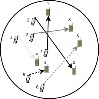
Figure 1: System Model

Algorithm 1 Game-Theoretic Distributed Channel Allocation

Parameters

1. Let $h_{m,n,k}$ be the channel gain of RE $k$ (time-frequency slot) between transmitter $m$ and receiver $n$.

2. Let $P_{n}$ be the transmission power of transmitter $n$.

3. Let $u_{n}\left(\boldsymbol{\mathbf{a}}\right)$ be the utility function of an FSIG $G$ (see Definition III.1).

Modified Fictitious Play (Section III.3)

1. Initialization - Choose $0<\alpha\leq 1$ and $\tau>0$. Each user picks a RE at random and then initializes his fictitious utility - $\bar{U}_{n,k}(0)=u_{n}\left(k,\boldsymbol{\mathbf{a}}_{-n}\left(0\right)\right)$ for each $k$.

2. At each turn $t>0$, each of the users $n=1,...,N$ does the following

   1. Chooses a transmission RE

      $$a_{n}(t)=\arg\underset{k}{\max}\,\overline{U}_{n,k}(t-1)$$

   2. Senses the interference at each RE $k$

      $$I_{k}(\boldsymbol{a}_{-n}\left(t\right))=\underset{m|a_{m}(t)=k}{\sum}|h_{m,n,k}|^{2}P_{m}$$

   3. Updates the fictitious utility for each RE $k$

      $$\overline{U}_{n,k}(t)=(1-\alpha)\overline{U}_{n,k}(t-1)+\alpha u_{n}\left(k,I_{k}\left(\boldsymbol{\mathbf{a}}_{-n}\left(t\right)\right)\right)$$

   4. (optional) Checks for convergence to a PNE of $G$. If $t\mod\tau=0$ and $I_{k}\left(\boldsymbol{\mathbf{a}}_{-n}\left(t\right)\right))\neq I_{k}\left(\boldsymbol{\mathbf{a}}_{-n}\left(t-1\right)\right))$ for some $k$ then set $\bar{U}_{n,k}(t)=0$ for each $k$.

II-A Channel Gain Assumptions

The channel between each transmitter and receiver is Gaussian frequency-selective. This models an environment where the multipath phenomenon creates a superposition of waves that makes some frequency bands better than others, independently between users. The channel gains (fading coefficients) are modeled as $N^{2}K$ random variables - one for each RE, each transmitter and each receiver. These channel gains incorporate both the geometry of the network (in their expectation) and multipath affects (in their realization). Each of the $K$ REs is a time-frequency slot. We denote the total number of time slots by $s$ and the total number of frequency bands by $b$, so $K=bs$. The channel gain between user $n_{1}$’s transmitter and user $n_{2}$’s receiver in RE $k$ is denoted $h_{n_{1},n_{2},k}$, for $k=1,...,K$. Without loss of generality, we assume that all the REs of the same frequency-band have consecutive indices. For example, $h_{n_{1},n_{2},1}$,…, $h_{n_{1},n_{2},s}$ have a common frequency band and are identical.

While assuming i.i.d. channel gains may facilitate the analysis, in practice the channel gains may not be statistically independent. Correlations between channel gains of different REs can occur if the REs have a common frequency band, or even have frequency bands with carrier frequencies that are closer than the coherence bandwidth of the channel. For a non-vanishing transmission rate, the bandwidth of a single frequency band must be non-decreasing with $N$. Hence, the coherence bandwidth of the channel is at most $d$ times larger than the frequency band, for some integer $d$ that is fixed with respect to $N$. For that reason, with $s$ time slots, only frequency bands with index $j$ such that $\left|i-j\right|\leq ds$ are correlated with the $i$-th frequency band. Both the time-division and the frequency-division correlation are well captured by the following notion.

Definition II.1.

A random process $\left\{X_{i}\right\}$ is said to be $m-$dependent if and only if for each $i,j$ such that $\left|i-j\right|>m$ the variables $X_{i}$ and $X_{j}$ are statistically independent.

Our assumptions regrading the channel gains are defined as follows.

Definition II.2.

Let $m$ be a non-negative integer. The channel gains $\left\{h_{n_{1},n_{2},k}\right\}$ are said to form an $m$-dependent frequency-selective channel if all the following conditions hold

1. For each $n_{1},n_{2}$, the variables $h_{n_{1},n_{2},1},\,...,\,h_{n_{1},n_{2},K}$ are identically distributed, where $h_{n_{1},n_{2},k}$ is a complex number and $\left|h_{n_{1},n_{2},k}\right|$ has zero probability to be zero.

2. For each $k=1,...,K$, the variables $h_{n_{1},n_{2},k}$ and $h_{n_{3},n_{4},k}$ are independent if $n_{1}\neq n_{3}$ or $n_{2}\neq n_{4}$.

3. For each $n_{1},n_{2}$, the variables $h_{n_{1},n_{2},1},\,...,\,h_{n_{1},n_{2},K}$ are $m$-dependent, i.e., for each $i,j$ such that $\left|i-j\right|>m$, the variables $h_{n_{1},n_{2},i}$ and $h_{n_{1},n_{2},j}$ are independent.

Specifically, we use the term independent frequency-selective channel instead of an $0$-dependent frequency-selective channel, since $h_{n_{1},n_{2},1},\,...,\,h_{n_{1},n_{2},K}$ are simply independent in this case.

The independence of channel gains of different users (Part 2 of Definition II.2) stems from their different physical locations (see Fig. 1), where the multipath pattern is different. As in MIMO transceivers, a distance of half a wavelength is far enough for the channel gains to be considered independent. For different users that typically are meters apart, this independence assumption is a common practice.

Note that $NK$ of the channel gains are between a transmitter and his designated receiver (a link). These channel gains are referred to as the direct channel gains. The other $NK(N-1)$ channel gains serve as interference coefficients between transmitters and unintended receivers. In a distributed ad-hoc network, we expect each user to have knowledge only on the channel gains he can measure, as formalized next.

Definition II.3 (CSI Knowledge Assumptions).

We assume that each user $n$ has perfect channel state information (CSI) of all his $K$ channel gains, $h_{n,n,1},...,h_{n,n,K}$. We also assume that each user knows the interference $I_{k}\left(\mathbf{a}_{-n}\right)=\underset{m|a_{m}=k}{\sum}|h_{m,n,k}|^{2}P_{m}$ he experiences in each RE $k$, where $P_{m}$ is the transmission power of user $m$. Users do not have any knowledge regarding the channel gains of other users and the specific interference coefficients.

In practice, user $n$ (transmitter-receiver pair) can estimate $h_{n,n,1},...,h_{n,n,K}$ by transmitting a wideband pilot sequence over the channels. The measurement of the aggregated interference is done in the receiver by directly measuring the incoming power at each frequency band. This requires from each device to have a wide-sensing capabilities, that are already practical in modern devices.

Mathematically, our channel gains are static random variables and not time-varying random processes. The implication of this model is that channel gains are constant with time. In practice, channel gains can only be assumed constant for a duration known as the coherence time of the channel. In a centralized system, acquiring the large number of channel gains is likely to take more time than the coherence time. Our fully distributed approach does not suffer from this limitation. However, for our channel allocation to be practical, we need an algorithm that converges to an allocation fast enough. If it converges much faster than the coherence time of the channel, it can be repeatedly updated in the network and maintain multi-user diversity. Although dynamics and convergence are not the emphasis of this work, we do show in simulations that Algorithm 1 converges very fast. This suggests that our algorithm can be considered practical in quasi-static environments like sensor networks and in-door networks, or in general in underspread systems which constitute a significant part of modern OFDM systems.

II-B Performance

Somewhat surprisingly, we show in this paper that asymptotically optimal performance can be achieved without the knowledge of the whole CSI in any part of the network. In fact, our algorithm does not require any communication at all between users. Our global performance metric is the weighted sum of achievable rates while treating interference as noise. We assume the following on the weights.

Definition II.4 (Bounded Weights).

We assume that the weights satisfy $w_{min}\leq w_{n}\leq w_{max}$ for some $w_{min},w_{max}>0$, for all $n$. Throughout this paper we refer to this assumption as “bounded weights”.

Our global performance metric is defined as follows.

Definition II.5.

Denote by $\mathbf{a}$ the allocation vector (the strategy profile), such that $a_{n}=k$ if user $n$ is using RE $k$. We want to maximize the following global performance function over all possible allocations

$$W\left(\mathbf{a}\right)=\sum_{n=1}^{N}w_{n}R_{n}\left(\mathbf{a}\right)=\sum_{n=1}^{N}w_{n}\log_{2}\left(1+\frac{P_{n}|h_{n,n,a_{n}}|^{2}}{N_{0}+I_{a_{n}}\left(\mathbf{a}_{-n}\right)}\right)$$ (1)

where $R_{n}\left(\mathbf{a}\right)$ is the achievable rate of user $n$, $N_{0}$ is the Gaussian noise variance in each receiver, $P_{n}$ is user $n$’s transmission power and $I_{k}\left(\mathbf{a}_{-n}\right)=\underset{m|a_{m}=k}{\sum}|h_{m,n,k}|^{2}P_{m}$ is the interference user $n$ experiences in RE $k$.

Each user first needs to measure his experienced interference $I_{a_{n}}\left(\mathbf{a}_{-n}\right)$ to be able to compute the achievable rate in (1) and devise his coding scheme accordingly. This can be done using a short preamble of pilots sent in the beginning of the transmission. Alternatively, the transmission scheme can be adapted using a fast enough feedback in the user’s link based on the bit-error rate experienced in the receiver.

Since our global performance metric includes the weights $\left\{w_{n}\right\}$, one would expect that they will appear as an input for the algorithm. This might be a tricky thing to do in a distributed algorithm, because it is not clear what is exactly the input and which user should know which weights. Fortunately, this dilemma is avoided in our case, and for a very satisfying reason. Our NE of the designed game have asymptotically optimal weighted sum-rate in $N$, regardless of the choice of weights as long as they are bounded (independent of $N$). This means that the NE maximize the sum-rate while maintaining some fairness between users. Only an asymptotically negligible amount of users might suffer from not close to optimal performance.

III Frequency-Selective Interference Games

We want to find a fully distributed way to achieve close to optimal solutions for our channel allocation problem. Hence we need to analyze the interaction that results from $N$ independent decision makers and ensure that the outcome is desirable. The natural way to tackle this problem is by applying game theory. A good overview of game theory can be found in [46]. The book by [30] provides a good overview of applications of game theory to communication. The two games we analyze in this work belong to the following family.

Definition III.1.

A frequency-selective interference game (FSIG) is a normal-form game

$$G=<\mathcal{N},\{A_{n}\}_{n\in\mathcal{N}},\{u_{n}\}_{n\in\mathcal{N}}>$$ (2)

where $\mathcal{N}$ is the set of users, which are transmitter-receiver pairs (links), $A_{n}$ is the set of the $K$ REs for all $n$, and $u_{n}:A_{1}\times...\times A_{N}\rightarrow\mathbb{R}$ is the utility function of user $n$, which is in the form

$$u_{n}\left(k,\boldsymbol{\mathbf{a}}_{-n}\right)=u_{n}\left(k,I_{k}\left(\boldsymbol{\mathbf{a}}_{-n}\right)\right)$$ (3)

where $I_{k}\left(\mathbf{a}_{-n}\right)$ is the interference user $n$ measures at RE $k$.

The utility form in (3) ensures that the utility can be computed independently by each user by measuring the interference in each RE (see the CSI Knowledge assumptions of Definition II.3). This is necessary in order to use $G$ for the distributed MAC protocol in Algorithm 1.

In the next subsection, we show that the stable points of Algorithm 1 are the pure NE of the FSIG the algorithm uses.

Definition III.2.

A strategy profile $(a_{n}^{*},\mathbf{a}_{-n}^{*})\in A_{1}\times...\times A_{N}$ is called a pure Nash equilibrium (PNE) if $u_{n}(a_{n}^{*},\mathbf{a}_{-n}^{*})\geq u_{n}(a_{n},\mathbf{a}_{-n}^{*})$ for all $a_{n}\in A_{n}$ and all $n\in\mathcal{N}$.

This means that for each player $n$, if the other players act according to the PNE, player $n$ can not improve his utility with another strategy. A game may exhibit a unique PNE, multiple PNE or none at all.

The utility functions are a design choice that we wish would induce a FSIG with only good NE in terms of the global performance of Definition II.5. The measure of success of the utility choice is given by the Pure Price of Anarchy (PPoA, see [16]), defined as follows.

Definition III.3.

The pure price of anarchy (PPoA) of a game $G=<\mathcal{N},\{A_{n}\}_{n\in\mathcal{N}},\{u_{n}\}_{n\in\mathcal{N}}>$ with the global performance function $W:A_{1}\times...\times A_{N}\rightarrow\mathbb{R}$ is $\frac{\underset{\mathbf{a}\in A_{1}\times...\times A_{N}}{\max}W(\mathbf{a})}{\underset{\mathbf{a}\in\mathcal{P}_{e}}{\min}W(\mathbf{a})}$, where $\mathcal{P}_{e}$ is the set of PNE.

A PPoA close to one means that the worst PNE of the game is close to the optimal solution. This is of great value since guaranteeing that the dynamics will avoid the worst equilibrium can be extremely hard, especially without any communication between the users (which we forbid in this work). Note that the PPoA is defined with respect to the global performance function (in our case given by Definition II.5) and not the sum of utilities. The choice of the utility function affects the PPoA only indirectly, by determining the PNE of the resulting game, and specifically the worst one among them.

Table I: Notations and symbols used throughout this paper.

$N$	Number of users
$K$	Number of REs (time-frequency slots)
$M$ (or $M_{N}$,$M_{K}$)	Number of best (or worst) REs for each user. Denoted $M_{N}$ (or $M_{K}$) where the dependence on $N$ (or $K$) is relevant
$\mathbf{a}$	Strategy profile (RE choices)
$\mathbf{a}_{-n}$	Strategy profile of user $n$’s rivals
$a_{n}$	User $n$’s action (RE)
$I_{k}\left(\mathbf{a}_{-n}\right)$	The interference user $n$ measures in RE $k$, given $\mathbf{a}_{-n}$
$u_{n}$	The utility function of user $n$
$h_{n,m,k}$	Channel gain between user $n$’s transmitter to user $m$’s receiver, in RE $k$
$P_{n}$	User $n$’s transmission power
$X_{\left(i\right)}$	The $i$-th smallest variable among $X_{1},...,X_{N}$
$\operatorname*{plim}$	Convergence in probability

III-A Convergence to a PNE in a Frequency-Selective Interference Game

Our games of interest are static games with static equilibria. However, the process of converging to these static equilibria in practice is of course dynamic. By designing a game with a PPoA close to one, we are guaranteed that the performance of any distributed channel allocation algorithm that converges to a PNE will be close to optimal. Therefore the algorithm that we are looking for is not tailored to our specific problem but rather has general properties of convergence to NE. A great deal of work has been done on learning algorithms for NE (see [47, 48, 49] and [50] for a summary). One of the best known candidates for this task is the Fictitious Play (FP) algorithm [51, 52]. In FP, each player keeps the empirical mean vectors of the frequencies each other player has played his actions, and plays his best response to this fictitious strategy.

Although it has a strong connection to NE, FP is not guaranteed to converge at all. Convergence has only been proven for some special games that do not include our game (for example see [53]). Even if FP converges, it may be to a mixed NE, which is undesirable as a channel allocation solution. Proving the convergence of best-response like dynamics (such as the FP) to a PNE in interference games is a challenging task that is outside the scope of this paper. However, our recent results [54, 55] show that convergence of approximate best-response dynamics in interference games happens with high probability, despite the fact that they are not potential games.

A fundamental problem when implementing FP is the information it requires. In a wireless network, not only does a user have hardly any information about the previous action of each other user, but he also barely knows how many users there are. This is the reason we require from our designed utility of the FSIG (in (3)) that the effect of the other users on the utility of a user can be measured by measuring the interference. Exploiting this property, in Algorithm 1 we adjust the FP to the wireless environment by modifying it such that each user keeps track of a fictitious utility vector instead of the empirical mean vector of the rivals’ strategy profiles.

Additionally, we provide a simple mechanism to improve the chances of convergence to a PNE. The strategy profile determines the interference, but knowing the interference will not reveal the strategy profile. Nevertheless, the continuity of the random channel gains suggests that for each user, the interference vector is different for different strategy profiles with probability 1. Hence users can detect that two strategy profiles are different based on their measured interference. If a PNE is reached it is played repeatedly, so we can exploit this fact and let the users check for convergence to a PNE after enough time, and set their fictitious utilities to zero if a PNE has not been reached. This gives Part d of Algorithm 1.

We assume time is divided into discrete turns, and that in each turn users choose actions simultaneously. The synchronization between the users is only assumed to simplify the presentation. In fact, rarely the dynamics of a game have to be synchronized in order to converge. We demonstrate in simulations the behavior of our algorithm in an asynchronized environment.

The Modified FP is described in detail in Algorithm 1, and its properties are summarized in the next proposition. Note that $\alpha=1$ corresponds to the best-response dynamics.

Proposition III.4.

Consider a FSIG $G$ where the $N$ users play according to Algorithm 1. If $\alpha=\frac{1}{t+1}$ or $\alpha$ is constant with time then

1. If a PNE is attained at $t_{0}$ it will be played for all $t>t_{0}$.

2. If the fictitious utility vectors converge, then the resulting strategy profile is a NE.

   1. If $\alpha=\frac{1}{t+1}$ then this might be a mixed NE.

   2. If $\alpha$ is constant with time , then this is a PNE.

3. If $\mathbf{a\in}A_{1}\mathbf{\times...\times}A_{N}$ is played for every $t>t_{1}$ then $\mathbf{a}$ is a PNE.

Proof:

Assume we are at turn $t=T$ and define $p_{i}=\sum_{t=1}^{T}\frac{I(\mathbf{a}_{-n}(t)=\mathbf{a}_{i,-n})}{T}$ for the rivals’ strategy profile $\mathbf{a}_{i,-n}$, where $I$ is the indicator function. For $\alpha=\frac{1}{t+1}$, the equivalence of the modified FP to the original FP immediately follows from

$$\sum_{i}p_{i}u_{n}(a_{n},\mathbf{a}_{i,-n})=\sum_{i}p_{i}u_{n}\left(a_{n},I\left(\mathbf{a}_{i,-n}\right)\right)=\frac{1}{T}\sum_{t=1}^{T}u_{n}\left(a_{n},I\left(\mathbf{a}_{-n}\left(t\right)\right)\right)$$ (4)

since $\sum_{i}p_{i}u_{n}(a_{n},\mathbf{a}_{i,-n})$ is the mean empirical utility according to the fictitious rival profile. Then, the result follows from [52].

Consider next the case of a constant $\alpha$. If a PNE $\mathbf{a^{*}}$ is attained at $t_{0}$ then $a_{n}^{*}(t_{0})=\arg\underset{k}{\max}\,u_{n,k}(t_{0})$ and also $a_{n}^{*}(t_{0})=\arg\underset{k}{\max}\,\overline{U}_{n,k}(t_{0}-1)$ for each $n\in\mathcal{N}$. Considering the update rule and because $a_{n}^{*}(t_{0})=\arg\underset{k}{\max\,}\overline{U}_{n,k}(t_{0}-1)=\arg\underset{k}{\max\,}u_{n,k}(t_{0})$ we get

$$\arg\underset{k}{\max}\,(1-\alpha)\overline{U}_{n,k}(t_{0}-1)+\arg\underset{k}{\max}\,\alpha u_{n,k}(t_{0})=\arg\underset{k}{\max\,}\overline{U}_{n,k}(t_{0})=a_{n}^{*}(t_{0}+1)$$ (5)

and so on, for each $t>t_{0}.$ If the fictitious utility vectors converge, then $\underset{t\rightarrow\infty}{\lim}\overline{U}_{n,k}(t)$ exists and is finite for each $k$ and $n$. From the update rule we get $\alpha\underset{t\rightarrow\infty}{\lim}\overline{U}_{n,k}(t)=\alpha\underset{t\rightarrow\infty}{\lim}u_{n,k}(t)$ for each $n,k$ which means $\underset{t\rightarrow\infty}{\lim}\overline{U}_{n,k}(t)=\underset{t\rightarrow\infty}{\lim}u_{n,k}(t)$ for constant $\alpha$. Consequently, for all $t>t_{1}$ for some large enough $t_{1}$, $a_{n}(t)=\arg\underset{k}{\max}\,\overline{U}_{n,k}(t)=\arg\underset{k}{\max}\,u_{n,k}(t)$ for each $n\in\mathcal{N}$ and hence $\mathbf{a}$ is a PNE. ∎

In Section VI we show numerically that the modified FP algorithm introduced in this section leads to a very fast convergence to a PNE in the M-FSIG.

III-B Asymptotic NE Analysis in the Number of Users

In this paper we analyze the probability for the existence of only good NE asymptotically in the number of users. This should not be confused with requiring $N$ (and $K$) to be extremely large. The right way to interpret our approach is - given a finite $N$ and an interference network of interest, what is the probability that our designed game exhibits only good NE? the larger $N$ the larger this probability is. Since a distribution over the ensemble of interference networks is a formal way of counting networks, an equivalent interpretation is - how many of the interference networks of size $N$ have only good NE in our designed game? Throughout this work, all of the proofs involve bounding the relevant probabilities for finite $N$. The values of $N$ for which close to optimal performance is guaranteed are in fact very reasonable. Already for $N=50$ the asymptotic effects take place, as can be verified by our bounds for finite $N$ and also via simulations (which suggest that even smaller values are enough).

Since we assumed that the number of users equals to the number of REs (i.e, $N=K$), taking the number of users to infinity also takes the number of REs to infinity. This does not mean that the bandwidth of each user needs to decrease with $N$. We do not deal with networks that are growing larger but with a fixed given large network, with a fixed bandwidth assignment for each channel. For those networks we bound from below the probability that only good NE exist. Although our channel allocation does not assume anything about the associated bandwidth considerations, we propose the following thought experiment to demonstrate why large networks, that use more bandwidth in total, always exist from a theoretical perspective. This is in addition to their practical existence, especially in sensor networks (see [56]).

Assume that ten operators have ten separated networks, operating in the same geographical area, each consists of $K=N=10$ users and REs. By joining their pool of REs together, due to the selectivity of the channel, users of operator A might find some REs of operator B to be much more attractive than their current ones, and vice versa. This gain is known as multi-user diversity. Our results both formalize this intuition and provide a new strong argument why large networks are to be preferred. This joining will allow them for a simple channel allocation algorithm that requires no communication or overhead from the network and achieves close to optimal performance. None of them could do so well on his own. The total bandwidth of the converged network is ten times larger than each of the original ones. The resulting network has $N=K=100$, where our asymptotic results are strongly valid.

Our approach can also be utilized to save bandwidth. Without a simple distributed solution that allows for a close to optimal channel allocation, a network operator might have to settle for an arbitrary allocation that ignores the selectivity of the channel. The optimal solution yields approximately twice the sum-rate obtained by a random allocation (for reasonable $N$ values, as observed in our simulations). If operators are interested in preserving their users demand, each of them can use only half of its bandwidth and obtain the same performance in the converged network.

This idea of converging networks demonstrates that large networks (in terms of both $N$ and $K$) do not necessarily imply a smaller bandwidth for each user. Of course that large networks do not really have to be created from the convergence of smaller networks. This is a theoretic idea that emphasizes the importance of viewing all users and REs as though they all belong to a single large network. It is analogous to the idea of analyzing the capacity of an interference channel as though the whole bandwidth is available, where in practice the spectrum of interest may be licensed to different operators.

III-C The Bipartite Graph of Users and Resources

The structure of our random NE is closely related to the structure of perfect matchings in random bipartite graphs. In this subsection we specify this bipartite graph and define the relevant terminology.

The key to observing the bipartite graph structure hidden in our game is by simply looking at the $M$ best (or worst) REs of each user, as determined by his direct channel gains alone. Throughout the paper, we denote by $h_{n,n,(N-i+1)}$ the channel gain with the $i$-th largest absolute value, which we refer to as the $i$-th best RE for user $n$ (so $h_{n,n,(1)}$ is the worst RE).

This information is conveniently described using a bipartite graph, defined as follows.

Definition III.5.

Let $B_{M}=\left(\mathcal{N},\mathcal{K},E\right)$ be a user-resource bipartite graph, where $\mathcal{N}$ is the set of user vertices, $\mathcal{K}$ is the set of resource vertices, and $E$ is the set of edges between them. An edge $e$ between user $n$ and RE $k$ exists ($e\in E$) if and only if RE $k$ is one of the $M$ best (or worst) REs of user $n$, i.e., $\left|h_{n,n,k}\right|\geq\left|h_{n,n,\left(N-M+1\right)}\right|$.

• The degree of a user or a RE is defined as the degree of its corresponding vertex in the graph.

• A matching in this graph is a subset of edges such that no more than a single edge is connected to each user vertex or RE vertex.

• A maximum matching is the matching with the maximal cardinality.

• A perfect matching is a maximum matching where all user and RE vertices are connected to a single edge (have degree one). It is feasible only with a balanced bipartite graph, where $\left|\mathcal{N}\right|=\mathcal{\left|K\right|}$ ($N=K$).

Note that $B_{M}$ represents the $M$-best (or worst) REs of each user, and not which RE is allocated to which user.

Since the channel gains are random, they induce a random bipartite graph. This raises the question of the probability for a perfect matching in this random bipartite graph. Due to the independency of channel gains between users, the edges connected to different user vertices are independent. However, the edges connected to the same user vertex are dependent.

Fig. 2 presents a toy example for a user-resource bipartite graph. Here each user vertex (a circle) is connected to two RE vertices (squares). The dotted edges represent a possible perfect matching in this graph. This perfect matching is a potential allocation of REs to users where there is no resource sharing. Alternatively, the gray edges represent another potential allocation (but not a matching) where RE 3 is shared between User 2 and User 4.

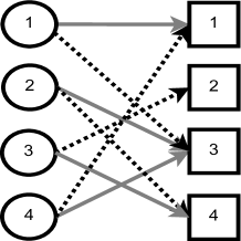
Figure 2: A toy example for a user-resource bipartite graph with $N=K=4$.

IV The Naive Frequency-Selective Interference Game Can Lead to Very Poor Performance

Our performance metric is the (weighted) sum of achievable rates. Hence, a natural choice for the utility of each user is his own term in the sum - his achievable rate. In a strategic or economical environment, this choice can be interpreted as the selfishness of the users. But we deal with devices that implement a protocol, that like any other, is wired in their circuits. This is a distributed protocol where each device maximizes the utility function we chose as designers. Choosing the achievable rate as the utility ignores the degree of freedom we have in designing the protocol by designing the utility. Therefore we name the resulting game the “naive game”. We show in this section that this naive choice for the utility can lead to poor global performance. This motivates a more careful choice for the utility.

Definition IV.1.

The Naive Frequency-Selective Interference Game (Naive-FSIG) is a normal-form game with $N$ users as players, where each has the set $A_{n}=\left\{1,2,...,K\right\}$ as a strategy space. The utility function for user $n$ is

$$u_{n}\left(\mathbf{a}\right)=R_{n}\left(\mathbf{a}\right)=\log_{2}\left(1+\frac{P_{n}|h_{n,n,a_{n}}|^{2}}{N_{0}+I_{a_{n}}\left(\mathbf{a}_{-n}\right)}\right).$$ (6)

We show in this section that with strong enough interference, the PPoA of the Naive-FSIG approach infinity (see Definition III.3). Strong interference is formally defined as follows

Definition IV.2.

The strong interference condition on the channel gains requires that for each $m$ and $l$

$$\frac{P_{m}}{N_{0}}\geq\underset{n,k}{\max}\frac{1}{\left|h_{m,n,l}\right|^{2}}\left(\frac{\left|h_{n,n,l}\right|^{2}}{\left|h_{n,n,k}\right|^{2}}-1\right).$$ (7)

Next we formalize the main theorem of this section. It shows that the Naive-FSIG is a bad choice for a game formulation aimed to provide a distributed solution for the channel allocation problem.

Theorem IV.3 (Naive-FSIG Main Theorem).

Let $\left\{h_{n_{1},n_{2},k}\right\}$ form an independent frequency-selective channel such that $\left|h_{n,n,1}\right|,\,...,\,\left|h_{n,n,k}\right|$ have a continuous distribution $F_{n}\left(x\right)$, with $F_{n}\left(x\right)>0$ for all $x>0$. If the strong interference condition (7) holds, then for all $\mu<1$ there are at least $\left(N^{\mu}\right)!$ PNE $\mathbf{a^{*}}$ such that

$$\operatorname*{plim}_{N\to\infty}\frac{1}{N}\sum_{n}w_{n}R_{n}\left(\mathbf{a^{*}}\right)=0$$ (8)

for any bounded weights $\left\{w_{n}\right\}$. Specifically, the PPoA of the Naive-FSIG approaches infinity in probability as $N\rightarrow\infty$.

The proof of the above theorem follows by analyzing the PNE of the Naive-FSIG for strong interference and evaluate the PPoA. The idea of this analysis, which is the proof strategy of Theorem IV.3, is explained here.

Trivially, a user who got his best RE without interference cannot improve his utility. On the other hand, a user who is not in his best RE (with the best channel gain) cannot necessarily improve his utility if there are users in his more preferable REs. The influence of other users in the RE of user $n$ on his utility is caused by the interference. Consequently, the strength of the interference has a crucial effect on the identity of the NE.

If the interference is strong enough, users in the same RE achieve a negligible utility and the interference game becomes a “collision game”. In such a collision game, every permutation between users and REs is a PNE, and every PNE is a permutation between users and REs. We formalize this idea in Lemma IV.4.

The strong interference condition (7) can also be written as

$$\frac{P_{m}}{N_{0}}\left|h_{m,m,l}\right|^{2}\geq\underset{n,k}{\max}\frac{\left|h_{m,m,l}\right|^{2}}{\left|h_{m,n,l}\right|^{2}}\left(\frac{\left|h_{n,n,l}\right|^{2}}{\left|h_{n,n,k}\right|^{2}}-1\right)$$ (9)

for each $m,l$. For large $N$, we expect $\frac{\left|h_{n,n,l}\right|^{2}}{\left|h_{n,n,k}\right|^{2}}$ to be large due to the order statistics that stem from maximizing over $n,k$. The rate of growth of the expectation due to order statistics is bounded from above by $O\left(\sqrt{N}\right)$ (it is usually much slower, e.g., $O\left(\ln N\right)$, see [57]). Hence, the strong interference condition is likely to hold when the expectation of the ratio $\frac{\left|h_{m,m,l}\right|^{2}}{\left|h_{m,n,l}\right|^{2}}$ decreases with $N$. This is naturally possible if the area where the users are located scales linearly with $N$ (constant user density). In particular, $\frac{\left|h_{m,m,l}\right|^{2}}{\left|h_{m,n,l}\right|^{2}}$ can decrease linearly with $N$ if transmitter $m$ is close to receiver $n$ and far from receiver $m$. In this case, a transmission power that grows at least like $O\left(\sqrt{N}\right)$ is necessary to obtain a reasonable SNR at the receiver, if the receiver is far away from the transmitter. Alternatively, if $P_{m}$ is high enough then (9) also holds. Hence, we conclude that the strong enough interference condition may hold due to geometrical considerations or working in the high-SNR regime.

Now we need to analyze the performance of the worst perfect matching. In Proposition IV.5 we show that a bad RE for a user can be asymptotically worthless, i.e., results in an achievable rate that goes to zero. This Proposition defines a bad RE as one of the worst $M_{N}$ such that $\underset{N\rightarrow\infty}{\lim}\frac{M_{N}}{N}=0$. Next we answer the question of how many users can get such a bad RE in a perfect matching. Unfortunately, all of them can. This is proved in Theorem IV.6 which is based on the theory of random bipartite graphs of users and REs introduced in Subsection III-C. This theory also allows us to show that there are many such bad perfect matchings (Theorem IV.7). In summary, we show that for strong enough interference there are many PNE (perfect matchings) which have a vanishing average achievable rate per user. Thus, the PPoA of the Naive-FSIG approaches infinity in the strong interference regime.

The following lemma shows that the set of PNE is the set of permutations between users and REs.

Lemma IV.4.

If the strong interference condition (7) holds, then the set of PNE of the Naive-FSIG is the set of perfect matchings between users and REs, with cardinality $N!$.

Proof:

Rearranging the inequality condition we get $\frac{1}{N_{0}}\underset{k}{\min}\left|h_{n,n,k}\right|^{2}>\underset{l}{\max}\frac{\left|h_{n,n,l}\right|^{2}}{N_{0}+\underset{m}{\min}\left(\left|h_{m,n,l}\right|^{2}P_{m}\right)}$ for each $n$. This directly means that for every strategy profile that is a permutation of users to REs, a user who deviates gets a lower utility. The interpretation of these inequalities is that the interference in the whole network is strong enough such that switching to an occupied RE is always worse than staying with an interference-free RE. Consequently, every permutation is an equilibrium. Conversely, every equilibrium must be a permutation because all users prefer an empty RE over a shared one (i.e. with positive interference). ∎

The lemma above implies that with strong enough interference, a PNE of the Naive-FSIG may assign some users a bad RE. The next proposition formulates this idea and shows that a bad RE can be asymptotically worthless.

Proposition IV.5.

Assume that $\left|h_{n,n,1}\right|,\,...,\,\left|h_{n,n,k}\right|$ are i.i.d. for each $n$, with a continuous distribution $F_{n}\left(x\right)$, such that $F_{n}\left(x\right)>0$ for all $x>0$. Let $M_{N}$ be a sequence such that $\underset{N\rightarrow\infty}{\lim}\frac{M_{N}}{N}=0$. If $m\leq M_{N}$ then $\underset{n}{\max}\left|h_{n,n,(m)}\right|\rightarrow 0$ in probability as $N\rightarrow\infty$.

Proof:

See Appendix A. ∎

Since $\frac{1}{N}\sum_{n}w_{n}R_{n}\left(\mathbf{a}\right)\leq w_{max}\underset{n}{\max\,}u_{n}$, it follows from the lemma above that the users that are assigned one of their $M_{N}$ worst channel gains have an average achievable rate that converges to zero in probability. To evaluate the performance of the worst PNE of the Naive-FSIG, we need to know how many users can be assigned such a bad RE. Unfortunately, there is an $M_{N}$ such that $\underset{N\rightarrow\infty}{\lim}\frac{M_{N}}{N}=0$, for which there exists a permutation between users and REs such that each user gets one of his $M_{N}$ worst channel gains. Even worse, there are actually many such permutations. This is shown by the following theorem.

Theorem IV.6.

Let $B_{M_{N}}$ be the bipartite user-resource graph of Definition III.5, where users are connected to their $M_{N}$-worst REs. Let $\left\{h_{n_{1},n_{2},k}\right\}$ form an independent frequency-selective channel. If $M_{N}\geq(e+\varepsilon)\ln(N)$ for some $\varepsilon>0$, then the probability that a perfect matching exists in $B_{M_{N}}$ approaches 1 as $N\rightarrow\infty$.

Proof:

See Appendix E. ∎

The condition $M_{N}\geq(e+\varepsilon)\ln(N)$ was necessary to ensure that with high probability, a perfect matching of users to bad REs exist. This large users’ node degree has its own major effect on the number of equilibria as well.

Theorem IV.7 (Marshall Hall Jr [58, Theorem 2]).

Suppose that $A_{1},A_{2},...,A_{N}$ are the finite sets of desirable resources, i.e. user $n$ desires resource $a$ if and only if $a\in A_{n}$. If there exists a perfect matching between users and resources and $\left|A_{n}\right|\geq M$ for $n=1\,,...,\,N$ where $M<N$, then the number of perfect matchings is at least $M!$.

The main theorem of this section (Theorem IV.3) readily follows by joining together Theorem IV.7, Lemma IV.4, Proposition IV.5 and Theorem IV.6 (choosing $M_{N}=N^{\mu}$ for some $\mu<1$).

V The M-Frequency Selective Interference Game is Asymptotically Optimal

The naive game introduced in the previous section has many bad equilibria for strong enough interference. Hence, using its utility as a distributed MAC protocol is a bad design choice. Our aim is to design an alternative artificial utility function that obtains good global performance (see Definition II.5). The restriction on this utility function is that it can be computed and maximized by each user independently such that no communication between users is required. This ensures that the resulting channel allocation protocol described in Algorithm 1 is fully distributed.

In general, it is intractable to find the optimal utility function (in terms of Definition II.5) without defining a manageable domain of search (such as in pricing mechanisms). Fortunately, in the channel allocation problem the optimal utility (asymptotically in the number of users) happens to be a slight modification of the naive selfish utility. In this new utility function defined below, we choose the utility of each user to be greater than zero only for his $M$ best REs, and be equal for them. We prove in this section that this subtle change of the utility in Definition IV.1 turns the tide for the performance of the PNE of the game. Instead of many asymptotically worthless equilibria for strong enough interference, we get that all equilibria are asymptotically optimal for any interference regime. For this reason, in this game, the convergence to some PNE is sufficient to provide asymptotically optimal global performance.

Definition V.1.

The M-Frequency-Selective Interference Game (M-FSIG) is a normal-form game with parameter $M>0$ and $N$ users as players, where each has the set $A_{n}=\left\{1,2,...,K\right\}$ as a strategy space. The utility function for user $n$ is

$$u_{n}\left(\mathbf{a}\right)=\left\{\begin{array}[]{cc}\log_{2}\left(1+\frac{P_{n}|h_{n,n,(K-M+1)}|^{2}}{N_{0}+I_{a_{n}}\left(\mathbf{a}_{-n}\right)}\right)&\frac{\left|h_{n,n,a_{n}}\right|}{\left|h_{n,n,(K-M+1)}\right|}\geq 1\\ 0&else\end{array}\right..$$ (10)

Define the set of indices of the $M$ best channel gains of user $n$ by $\mathcal{M}_{n}=\left\{k\,|\,\frac{\left|h_{n,n,k}\right|}{\left|h_{n,n,(K-M+1)}\right|}\geq 1\right\}.$ Note that because $\frac{P_{n}|h_{n,n,(K-M+1)}|^{2}}{N_{0}+I_{a_{n}}\left(\mathbf{a}_{-n}\right)}>0$ for each $n\in\mathcal{N}$ with probability 1, user $n$ will never choose a RE outside $\mathcal{M}_{n}$. This means that this utility causes users to practically limit their chosen strategies to the smaller set of their $M$-best REs.

Also note that due to the replacement of $h_{n,n,a_{n}}$ by $h_{n,n,(K-M+1)}$ in the utility, we obtain that

$$\arg\underset{a_{n}}{\max\,}u_{n}\left(\mathbf{a}\right)=\arg\underset{a_{n}\in\mathcal{M}_{n}}{\min}I_{a_{n}}\left(\mathbf{a}_{-n}\right).$$ (11)

Hence in the M-FSIG each user $n\in\mathcal{N}$ only accesses REs in $\mathcal{M}_{n}$ and prefers those with smaller interference.

We refer to this designed utility as a slight modification of the utility of the Naive-FSIG (given in Definition IV.1) since for each one of the $M$-best REs, the ratio of (6) and (10) approaches one as $N$ approaches infinity. This is due to $\frac{\left|h_{n,n,(K-M+1)}\right|}{\left|h_{n,n,(K)}\right|}\rightarrow 1$ as $N\rightarrow\infty$ for a broad class of fading distributions, as we prove in this section. Somewhat ironically, although in this game each user is not exactly maximizing his own achievable rate, his achievable right in equilibrium is going to be better maximized than in the Naive-FSIG.

The above designed utility requires less information than a utility that considers only REs that are better than some threshold (as in [39]). A threshold that avoids asymptotic performance loss has to depend on $K$, where the dependence is determined by the fading distribution. However, the fading distribution is not likely to be known to the users. Furthermore, the above utility only requires each user to track a small number of REs ($O\left(\ln K\right)$ instead of $K$).

Naturally, the asymptotic optimality of the M-FSIG depends on the distribution of the channel gains. In order to capture the general nature of fading distributions, we define the following class. The properties of these distributions that are useful for this section’s results are analyzed in Appendix B.

Definition V.2 (Exponentially-Dominated Tail Distribution).

Let $X$ be a random variable with a continuous CDF $F_{X}$. We say that $X$ has an exponentially-dominated tail distribution if there exist $\alpha>0,\beta\in\mathbb{R\text{ }},\lambda>0,\gamma>0$ such that

$$\underset{x\rightarrow\infty}{\lim}\frac{1-F_{X}\left(x\right)}{\alpha x^{\beta}e^{-\lambda x^{\gamma}}}=1.$$ (12)

The main theorem of this section shows that the pure price of anarchy of the M-FSIG is asymptotically optimal for fading coefficients with an exponentially-dominated tail, under the right choice of the parameter $M$, defined as follows.

Theorem V.3 (M-FSIG Main Theorem).

Let $\left\{h_{n_{1},n_{2},k}\right\}$ form an $m$-dependent frequency-selective channel. If, for each $k$, $\left|h_{n,n,k}\right|$ has an exponentially-dominated tail and $M=\left(m+1\right)(e+\varepsilon)\ln K$ for some $\varepsilon>0$ then

$$\operatorname*{plim}_{N\to\infty}\frac{\underset{\mathbf{a}\in A_{1}\times...\times A_{N}}{\max}W(\mathbf{a})}{\underset{\mathbf{a}\in\mathcal{P}_{e}}{\min}W(\mathbf{a})}=1$$

where $\mathcal{P}_{e}$ is the set of pure NE of the M-FSIG and $W(\mathbf{a})=\sum_{n}w_{n}R_{n}\left(\mathbf{a}\right)$ is the weighted sum of achievable rates with bounded weights (see Definition II.5).

Proof:

From Corollary V.4 we know that for $M=\left(m+1\right)\left(e+\varepsilon\right)\ln K$, there asymptotically exist many PNE in the M-FSIG, with high probability. Denote by $\mathcal{S_{\tilde{\mathbf{a}}}}$ the set of sharing users in $\tilde{\mathbf{a}}=\arg\underset{\mathbf{a}\in\mathcal{P}_{e}}{\min}W(\mathbf{a})$. From Proposition V.7 we know that for every $\mathbf{a}^{*}\in\mathcal{P}_{e}$

$$\frac{W(\mathbf{\mathbf{a}^{*}})}{\underset{\mathbf{a}\in A_{1}\times...\times A_{N}}{\max}W(\mathbf{a})}\geq\frac{\sum_{n\in\mathcal{\mathcal{N}\setminus\mathcal{S_{\tilde{\mathbf{a}}}}}}w_{n}\log_{2}\left(1+\frac{P_{n}}{N_{0}}\left|h_{n,n,(K-M+1)}\right|^{2}\right)}{\sum_{n\in\mathcal{\mathcal{N}}}w_{n}\log_{2}\left(1+\frac{P_{n}}{N_{0}}\left|h_{n,n,(K)}\right|^{2}\right)}\geq\\ \frac{\sum_{n\in\mathcal{\mathcal{N}\setminus\mathcal{S_{\tilde{\mathbf{a}}}}}}w_{n}\underset{m}{\min}\log_{2}\left(1+\frac{P_{m}}{N_{0}}\left|h_{m,m,(K-M+1)}\right|^{2}\right)}{\sum_{n\in\mathcal{\mathcal{N}}}w_{n}\underset{m}{\max}\log_{2}\left(1+\frac{P_{m}}{N_{0}}\left|h_{m,m,(K)}\right|^{2}\right)}=\underbrace{\frac{\sum_{n\in\mathcal{\mathcal{N}\setminus\mathcal{S_{\tilde{\mathbf{a}}}}}}w_{n}}{\sum_{n\in\mathcal{\mathcal{N}}}w_{n}}}_{A}\underbrace{\frac{\underset{m}{\min}\log_{2}\left(1+\frac{P_{m}}{N_{0}}\left|h_{m,m,(K-M+1)}\right|^{2}\right)}{\underset{m}{\max}\log_{2}\left(1+\frac{P_{m}}{N_{0}}\left|h_{m,m,(K)}\right|^{2}\right)}}_{B}\underset{\begin{array}[]{c}N\rightarrow\infty\\ (a)\end{array}}{\rightarrow}1$$ (13)

where (a) follows since for $M=\left(m+1\right)\left(e+\varepsilon\right)\ln K$:

• In Theorem V.6 (Section V.I) we prove that for every PNE of the M-FSIG , and specifically the worst one, $\frac{\left|\mathcal{\mathcal{S_{\tilde{\mathbf{a}}}}}\right|}{N}\rightarrow 0$ as $N\rightarrow\infty$. Hence $A\rightarrow 1$ as $N\rightarrow\infty$, due to

  $$1\geq\frac{\sum_{n\in\mathcal{\mathcal{N}\setminus\mathcal{S_{\tilde{\mathbf{a}}}}}}w_{n}}{\sum_{n\in\mathcal{\mathcal{N}}}w_{n}}=A=1-\frac{\sum_{n\in\mathcal{\mathcal{S_{\tilde{\mathbf{a}}}}}}w_{n}}{\sum_{n\in\mathcal{\mathcal{N}}}w_{n}}\geq 1-\frac{\left|\mathcal{\mathcal{S_{\tilde{\mathbf{a}}}}}\right|}{N}\frac{w_{\max}}{w_{\min}}\underset{\begin{array}[]{c}N\rightarrow\infty\end{array}}{\rightarrow}1.$$ (14)

• In Theorem V.11 (Section V.II) we prove that $B\rightarrow 1$ as $N\rightarrow\infty$.

∎

In the following two subsections we prove Theorem V.6 and Theorem V.11 that are necessary for our main Theorem above. The first subsection is about the structure of the PNE of the M-FSIG. We show in Theorem V.6 that all of the PNE of the M-FSIG are almost a perfect matching in between users and $M$-best REs, so almost all users obtain an interference-free RE. The second subsection is about the weighted sum-rate performance of the PNE of the M-FSIG. We show in Theorem V.11 that for exponentially-dominated tail distributions and $m$-dependent REs, in all PNE of the M-FSIG, even the minimal rate of a user is asymptotically optimal, provided that this user is in an interference-free RE.

V-A Asymptotic Existence and Structure of the Equilibria

In this subsection we argue about the structure of the PNE of the M-FSIG using two complementary results. The first shows that there are many PNE which are perfect matchings between users and $M$-best REs. The second shows that a PNE that is far from a perfect matching cannot asymptotically exist. Together we conclude that all PNE are almost "at least" a perfect matching.

Using the existence Theorem for a perfect matching in Appendix E together with Theorem IV.7 we get the following corollary.

Corollary V.4.

Let $B_{M}$ be the bipartite user-resource graph of Definition III.5, where users are connected to their $M$-best REs. Let $\left\{h_{n_{1},n_{2},k}\right\}$ form an $m$-dependent frequency-selective channel. If the M-FSIG parameter is chosen such that $M\geq\left(e+\varepsilon\right)\left(m+1\right)\ln(N)$ for some $\varepsilon>0$, then the probability that there are at least $M!$ perfect matchings in $B_{M}$ approaches 1 as $N\rightarrow\infty$.

It turns out that the asymptotically optimal PNE are typical equilibria for this game; in other words all other equilibria have almost the same asymptotic structure, which is a perfect matching. This property eases the requirements for the dynamics and allows simpler convergence with good performance.

Definition V.5.

Define a shared RE as a RE that is chosen by more than one user. Define a sharing user as a user that chose a shared RE.

Theorem V.6.

Let $\left\{h_{n_{1},n_{2},k}\right\}$ form an $m$-dependent frequency-selective channel. Suppose that $M\geq\left(e+\varepsilon\right)\left(m+1\right)\ln(N)$ for some $\varepsilon>0$. If $\mathbf{a^{*}}$ is a PNE of the M-FSIG with $N_{c}$ sharing users, then $\frac{N_{c}}{N}\rightarrow 0$ in probability as $N\rightarrow\infty$. Furthermore, $\underset{\mathbf{a^{*}}\in\mathcal{P}_{e}}{\max}\frac{N_{c}\left(\mathbf{a^{*}}\right)}{N}\rightarrow 0$ in probability as $N\rightarrow\infty$, where $\mathcal{P}_{e}$ is the set of pure NE.

Proof:

See Appendix C. ∎

By the definition of the M-FSIG, the achievable rate of a non-sharing user is close to optimal (attained in the best REs for zero interference). According to Theorem V.6 above, almost all of the users are non-sharing users. Consequently, almost all users have almost optimal performance. On the other hand, the sharing users do not necessarily suffer from poor performance: their chosen RE, although shared, has the minimal interference among the $M$ available REs. If $M$ is increasing with $N$, this minimal interference might not be large at all.

V-B Asymptotic Optimality of the Equilibria - Order Statistics of Fading Channels

In the last subsection we proved that all the PNE of the M-FSIG have the same structure asymptotically, which is “almost a perfect matching” between users and REs, such that each user gets one of his $M$-best REs. In this subsection we want to evaluate the global performance (see Definition II.5) of such an “almost perfect matching”. Since we measure the merits of the equilibria via the pure price of anarchy, we are interested in where does $\frac{\underset{\mathbf{a}\in\mathcal{P}_{e}}{\min}W(\mathbf{a})}{\underset{\mathbf{a}\in A_{1}\times...\times A_{N}}{\max}W(\mathbf{a})}\rightarrow 1$ as $N\rightarrow\infty$ for bounded weights (see Definition II.4).

At first glance it may seem that such analysis would involve the identity of the PNE and the optimal value of the global performance function $W(\mathbf{a})$, and thus could be quite tiresome. Fortunately, the definition of the M-FSIG and the “almost perfect matching” structure of its PNE allow for a simpler approach.

Proposition V.7.

Denote by $\mathcal{S_{\tilde{\mathbf{a}}}}$ the set of sharing users in $\tilde{\mathbf{a}}=\arg\underset{\mathbf{a}\in\mathcal{P}_{e}}{\min}W(\mathbf{a})$. The PPoA of the M-FSIG satisfies

$$\frac{1}{PPoA}=\frac{\underset{\mathbf{a}\in\mathcal{P}_{e}}{\min}W(\mathbf{a})}{\underset{\mathbf{a}\in A_{1}\times...\times A_{N}}{\max}W(\mathbf{a})}\geq\frac{\sum_{n\in\mathcal{\mathcal{N}\setminus\mathcal{S_{\tilde{\mathbf{a}}}}}}w_{n}\log_{2}\left(1+\frac{P_{n}}{N_{0}}\left|h_{n,n,(K-M+1)}\right|^{2}\right)}{\sum_{n\in\mathcal{\mathcal{N}}}w_{n}\log_{2}\left(1+\frac{P_{n}}{N_{0}}\left|h_{n,n,(K)}\right|^{2}\right)}.$$ (15)

Proof:

By definition of the M-FSIG, for each PNE $\mathbf{a^{*}}$ the inequality $W(\mathbf{a^{*}})\geq\sum_{n\in\mathcal{\mathcal{N}\setminus S_{\mathbf{a^{*}}}}}w_{n}\log_{2}\left(1+\frac{P_{n}}{N_{0}}\left|h_{n,n,(K-M+1)}\right|^{2}\right)$ holds (note that $\mathcal{\mathcal{N}\setminus S_{\mathbf{a^{*}}}}$ is the set of non-sharing users in $\mathbf{a^{*}}$). By the definition of the channel allocation problem $W(\mathbf{a})\leq\sum_{n\in\mathcal{N}}w_{n}\log_{2}\left(1+\frac{P_{n}}{N_{0}}\left|h_{n,n,(K)}\right|^{2}\right)$ holds for each $\mathbf{a}\in A_{1}\times...\times A_{N}$. By choosing $\tilde{\mathbf{a}}=\arg\underset{\mathbf{a}\in\mathcal{P}_{e}}{\min}W(\mathbf{a})$ in the first inequality and $\mathbf{a_{opt}}=\arg\underset{\mathbf{a}\in A_{1}\times...\times A_{N}}{\max}W(\mathbf{a})$ in the second we reach our conclusion. ∎

The proposition above suggests that if $\left|h_{n,n,(K-M+1)}\right|$ is asymptotically close, in some sense, to $\left|h_{n,n,(K)}\right|$, and $\sum_{n\in\mathcal{S_{\tilde{\mathbf{a}}}}}\left|h_{n,n,(K)}\right|$ is asymptotically negligible compared to $\sum_{n\in\mathcal{N}\setminus\mathcal{S_{\tilde{\mathbf{a}}}}}\left|h_{n,n,(K)}\right|$, then the PPoA of the M-FSIG converges to 1 in probability as $K\rightarrow\infty$. This leads us to explore the asymptotic statistical behavior of $|h_{n,n,(K-M+1)}|$ and $|h_{n,n,(K)}|$. Therefore a statistical equilibrium analysis is replaced by an order statistics analysis of the channel gains, which is much simpler.

For each $n\in\mathcal{N}$, Let $X_{n,1},X_{n,2},...,X_{n,K}$ be a sequence of random variables. We denote by $X_{n,(i)}$ the $i$-th variable in the sorted list of $X_{n,1},X_{n,2},...,X_{n,K}$, with increasing order, i.e. $X_{n,(1)}\leq X{}_{n,(2)}\leq...\leq X{}_{n,(K)}$. The statistics of $X_{n,(i)}$ are called the order statistics. We are interested in the statistics of $X_{n,(K-M_{K}+1)}$ for a sequence $M_{K}$ such that $\underset{K\rightarrow\infty}{\lim}\frac{M_{K}}{K}=0$ and $\underset{K\rightarrow\infty}{\lim}M_{K}=\infty$. (i.e. intermediate statistics) versus those of $X_{n,(K)}$ (i.e. extreme statistics). We assume for simplicity that $\left\{X_{n,k}\right\}$ are identically distributed; hence, we choose them as normalized channel gains.

Now we turn to characterize the distributions that we are interested in. The first distinction we have to make is between bounded and unbounded random variables.

Remark V.8 (Bounded Random Variables).

If $F_{X}^{-1}(1)<\infty$ then $X$ is a bounded random variable. In that case the behavior of $X_{n,(K-M_{K}+1)}$ compared to that of $X_{n,(K)}$ for a sequence $M_{K}$ such that $\underset{K\rightarrow\infty}{\lim}\frac{M_{K}}{K}=0$ and $\underset{K\rightarrow\infty}{\lim}M_{K}=\infty$ is much simpler to analyze. By substituting $\left|h_{n,n,k}\right|=F_{X}^{-1}(1)-X_{n,k}$ in Proposition IV.5, (assuming independent variables and a continuous distribution) we obtain $\underset{n}{\max}\left(F_{X}^{-1}(1)-X_{n,(K-M_{K}+1)}\right)\rightarrow 0$ as $K\rightarrow\infty$, hence $X_{n,(K-M_{K}+1)}-X_{n,(K)}\rightarrow 0$ for all $n$ in probability as $K\rightarrow\infty$. This immediately validates all the results of this section for bounded random variables.

Keeping the above remark in mind, we formulate our results assuming unbounded variables. Note that all the classical fading distributions are indeed unbounded. We are interested in proving our results for a large class of fading distributions, which evidently tend to belong to the family of exponentially-dominated tail distributions (see Definition V.2). Appendix B provides the necessary properties of exponentially-dominated distributions that we use for our following results. Note that the following results are true for $m$-dependent REs, that includes i.i.d. REs as a special case.

We start by proving that, for exponentially-dominated tail distributions, the ratio of the intermediate statistics to the extreme statistics approaches one as the number of REs approaches infinity. It shows that for a slow enough increasing $M_{K}$, the interference-free $M_{K}$ best RE of a user is asymptotically optimal in ratio.

Theorem V.9.

Let $X_{1},X_{2},...,X_{K}$ be unbounded $m$-dependent random variables with an exponentially-dominated tail. Let $M_{K}$ be a sequence such that $\underset{K\rightarrow\infty}{\lim}M_{K}=\infty$. If $\underset{K\rightarrow\infty}{\lim}\frac{M_{K}}{\ln^{\mu}K}=0$ for some $\mu<1$ then $\frac{X_{(K-M_{K}+1)}}{X_{(K)}}\rightarrow 1$ in probability as $K\rightarrow\infty$.

Proof:

See Appendix C. ∎

The following simple proposition shows that under the conditions of Theorem V.9, the achievable rate of the interference-free $M_{K}$ best RE is also asymptotically optimal in ratio.

Proposition V.10.

If $\frac{X_{(K-M_{K}+1)}}{X_{(K)}}\rightarrow 1$ in probability as $K\rightarrow\infty$ then for each $a>0$, $\frac{\log_{2}\left(1+\frac{P}{N_{0}}aX_{(K-M_{K}+1)}\right)}{\log_{2}\left(1+\frac{P}{N_{0}}aX_{(K)}\right)}\rightarrow 1$ in probability as $K\rightarrow\infty$.

Proof:

From the monotonicity of $\frac{\log_{2}\left(1+x\right)}{x}$ for $x>0$ it follows that $\frac{X_{(K-M_{K}+1)}}{X_{(K)}}\leq\frac{\log_{2}\left(1+\frac{P}{N_{0}}aX_{(K-M_{K}+1)}\right)}{\log_{2}\left(1+\frac{P}{N_{0}}aX_{(K)}\right)}$. ∎

Theorem V.9 implies that for almost all users $\frac{X_{n,(K-M_{K}+1)}}{X_{n,(K)}}\rightarrow 1$ as $K\rightarrow\infty$. In fact, because our global performance measure is logarithmic with respect to the channel gain power, a stronger result holds. The next theorem suggests that every non-sharing user enjoys asymptotically similar conditions. More formally, the minimal rate achieved by the non-sharing users is asymptotically optimal (maximized), which is known also as Max-min fairness between these non-sharing users. This shows that the perfect matching equilibria of the M-FSIG has Max-min fairness between all users. Note that the fact there is a perfect matching with performance that approaches the optimal solution for $W(\mathbf{a})$ means that a perfect matching can achieve the maximal multi-user diversity.

Theorem V.11 (Max-Min Fairness for non-sharing users).

Let $\left\{X_{n,k}\right\}$ be identically distributed unbounded random variables with an exponentially-dominated tail. Assume that $\left\{X_{n,k}\right\}_{k}$ are $m$-dependent for each $n$. Let $M_{K}$ be a sequence such that $\underset{K\rightarrow\infty}{\lim}M_{K}=\infty$. Let $a_{n}$ be a positive sequence. If $\underset{K\rightarrow\infty}{\lim}\frac{M_{K}}{K^{\mu}}=0$ for some $\mu<1$ then

$$\operatorname*{plim}_{K\to\infty}\frac{\underset{n}{\min}\log_{2}\left(1+\frac{P_{n}}{N_{0}}a_{n}X_{n,(K-M_{K}+1)}\right)}{\underset{n}{\max}\log_{2}\left(1+\frac{P_{n}}{N_{0}}a_{n}X_{n,(K)}\right)}=1.$$

Proof:

See Appendix C. ∎

The role of the sequence $a_{n}$ is to allow for $a_{n}X_{n,k}$ to have non identical parameters for different users, by choosing $X_{n,k}=\frac{\left|h_{n,n,k}\right|^{2}}{a_{n}}$.

VI Simulation Results

Our NE analysis in this paper is probabilistic and asymptotic with the number of users $N$. It provides bounds in terms of $N$ on the probability that all NE are asymptotically optimal. Simulations provide another assessment about of which $N$ values are enough for the asymptotic effects to hold. Since some of our bounds are not tight, simulations suggest that even smaller values of $N$ are enough.

In our simulations we used a Rayleigh fading network; i.e. $\left\{\left|h_{m,n,k}\right|\right\}$ are independent Rayleigh random variables. Hence $\left\{\left|h_{m,n,k}\right|^{2}\right\}$ are independent exponential random variables. The parameters $\left\{\lambda_{m,n}\right\}$ for the exponential variables were chosen according to the users’ random positions such that $\lambda_{m,n}=\frac{G}{r_{m.n}^{\gamma}}$, where $r_{m,n}$ is the distance between transmitter $m$ and receiver $n$, $\gamma$ is the path-loss exponent (which is chosen to be $\gamma=3$), and $G=\left(\frac{\lambda_{wave}}{4\pi}\right)^{\gamma}$ where $\lambda_{wave}$ is the wavelength (chosen to be $\lambda_{wave}=\frac{3\cdot 10^{8}}{2.4\cdot 10^{9}}$). The users’ receiver positions are chosen uniformly at random on a disk with radius $R=1000[m]$, and each transmitter position is at distance $R_{link}\sim N\left(50,25\right)$ (normally distributed) and angle $\theta\sim U\left([0,2\pi]\right)$ from its intended receiver. The transmission powers were chosen such that the mean SNR for each link, in the absence of interference, is 15[dB]. Users play according to the Modified FP algorithm (Algorithm 1) including Step d with $\tau=60$ and $\alpha=0.5$. The parameters for the simulations are summarized in Table II.

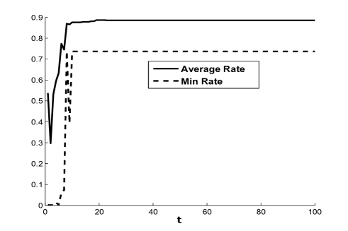
Figure 3: Sum-rate and min-rate compared to the optimal permutation allocation for a single realization in the uncorrelated case.

In Fig. 3 we present a typical convergence of the Modified FP for a single game realization with $N=50$ and $M=8$. Clearly convergence is very fast and occurs within 20 iterations. The ratio of the sum of achievable rates to that of an optimal allocation is close to 1, and the ratio of the minimal achievable rate is not far behind. This corresponds to a convergence to a PNE with two sharing users. These users do not decrease the minimal rate significantly, as they are the best choice among $M=8$ for each other. The geometry of the scenario allows for the minimal interferer to be far away.

In Fig. 4 we present again a typical convergence for a single game realization, but this time where users act asynchronously. In each turn a user is chosen at random among all the $N$ users to perform the Modified FP. In time $t$, the non-acting users keep their variables, described in Algorithm 1, fixed. The algorithm converges to a PNE with a similar performance and convergence rate to the synchronous case. Convergence time is approximately 50 times larger simply because now only a single user acts each turn instead of $N=50$ users. This figure demonstrates that synchronization is not an issue for our channel allocation algorithm.

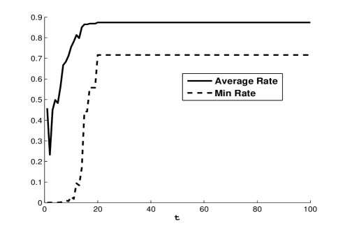
Figure 5: Modified FP convergence in a single realization in the $m$-dependent case.

Fig. 5 shows the convergence in a single network realization, for $N=50$ and $M=12$, for the case of the $m$-dependent frequency-selective channel. The direct channel gains of each user were generated using the Extended Pedestrian A model (EPA, see [59]) for the excess tap delay and the relative power of each tap. The parameter $m$ of their dependency is roughly given by $m\geq\frac{T_{s}N}{50\sigma_{\tau}}$ where $T_{s}$ is the duration of a symbol and $\sigma_{\tau}$ is the delay spread of the channel, which is $143[nsec]$. We chose $T_{s}=0.44[\mu sec]$ so $m=3$. As expected, the behavior is very similar to the uncorrelated case. The convergence time was unaffected and the sum and min rate were only slightly reduced. Note that the resulting pure NE is a perfect matching, (i.e., has no sharing users).

In Fig. 6 we show the effect of the number of users on the rates, with $M=\left\lceil 3\ln N\right\rceil$, averaged over 100 realizations. Only for $N=10$ we chose $M=5$. We present the average and minimal achievable rates, compared to the sum-rate optimal permutation allocation and random permutation allocation mean achievable rates. The benefit over a random permutation is significant, especially in terms of the minimal rate. The rate increase is due to the growing expected value of the best channel gain for each user. This phenomenon (multi-user diversity) of course does not take place for a random permutation. In a random permutation the average user gets his median channel gain, and the minimal allocated channel gain has a decreasing expectation. The random permutation may be interpreted as a result of a channel allocation scheme that ignores the selectivity of the channel, or as a random PNE of the Naive-FSIG for strong enough interference. The standard deviations of the mean rates are small as expected from the similarity of all NE, and the standard deviations of the minimal rate are higher due to the changing number of sharing users between different realizations.

In Fig. 7 we present the empirical cumulative distribution functions of the modified FP convergence time, that were derived from 100 realizations. Five different functions are depicted, for $N=10,100,200,300,400$, and $K=N$. We see that about 90% of the dynamics converge in less than 40 iterations. We can also see that the convergence time is very weakly affected by the number of users, which means the modified FP has excellent scalability properties.

Interestingly, the two last figures suggest that the asymptotic effects are starting to become valid already for small values of $N$. For $N=10$, ~85% of the realizations lead to convergence within 20 iterations, which is typical for larger $N$ values. The rest ~15% of realizations lead to convergence within 140 iterations. This “anomaly” shrinks significantly for larger $N$ values. The sum-rate was ~80% of the optimal, where multi-user diversity is still not significant for $N=10$. All the resulting PNE consist of zero or two sharing users, which coincides with the fact that all PNE are almost perfect matchings in the associated bipartite graph.

Finally, we compare the performance of Algorithm 1 to the distributed auction algorithm of [40] and the stable matching algorithm of [42]. In Fig. 9 we present the mean and minimal rates of these algorithms as a function of $N$, averaged over 100 realizations and for $N=25,50,75,100,125,150$. In Fig. 8 we present the empirical CDF of the convergence times for the experiment with $N=125$. The distributed auction algorithm is $\varepsilon$-optimal and we chose $\varepsilon=\frac{1}{N}$, so it naturally achieves the same rates (sum-rate and minimal) as the Hungarian algorithm in previous simulations. However, its convergence rate is more than one hundred times slower than that of Algorithm 1. Since a distributed channel allocation algorithm has to coverage within the coherence time of the channel, this slow convergence time is very restricting in practice. The stable matching algorithm always converges within a single contention window, assuming synchronized users. Our convergence time is naturally slower, but still very fast and does not require synchronized users (as demonstrated in Fig. 4). Our sum-rate is very similar to that of the stable matching algorithm, but the minimal rate is more than three times better. The stable matching algorithm has no fairness guarantees, and as indicated by the large error bars, results in a very different minimal rate in different networks. In fact, it may even choose not to assign any REs to some users, making the minimal rate zero. Nevertheless, these appealing performance improvements are not the main advantage of our algorithm over the existing ones. Both the distributed auction algorithm and the stable matching require that all users can hear all other users (fully connected network) so they can listen before transmission in a CSMA manner. This significantly limits the distributed nature of the network. In Algorithm 1, every user transmits in the RE that suits his utility best without considering any other user or avoiding a collision. Still, the overall performance is not only not worse but significantly better. This strengthens our claim that using utility design tools for distributed optimization can lead to much better distributed algorithms.

Table II: Simulation network parameters.

$\gamma$	Path-loss exponent	3
$\lambda_{wave}$	Wavelength (in meters)	$\frac{1}{2.4}10^{-9}$
SNR	(in the absence of interference)	15[dB]
$R$	Radius of the disk region (in meters)	$1000$
$R_{link}$	Distance between a transmitter and receiver pair	$\sim N\left(50,25\right)$
$\tau$	Modified FP NE check time	60
$\alpha$	Modified FP step size	0.5

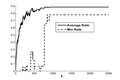
Figure 4: Asynchronized modified FP convergence in a single realization.

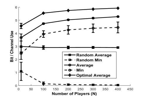
Figure 6: Rates as a function of $N$ averaged over 100 realizations.

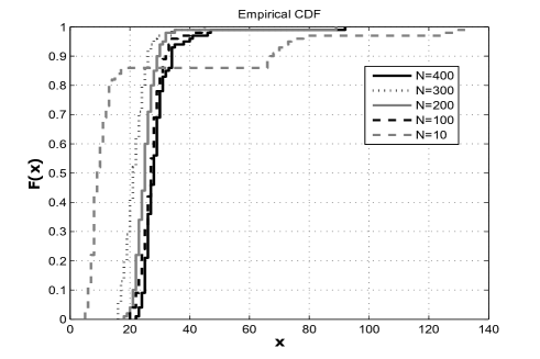
Figure 7: Empirical cumulative distribution functions of the convergence time for different $N$ values, over 100 realizations.

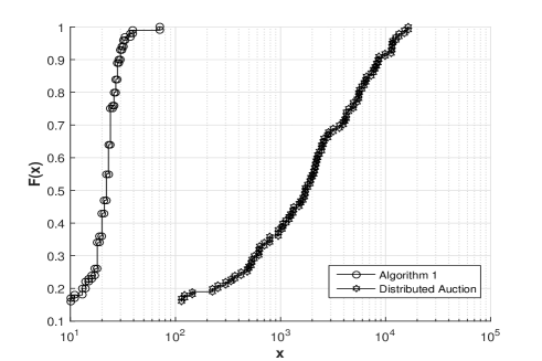
Figure 8: Empirical cumulative distribution functions of the convergence time for $N=125$ over 100 realizations, compared to state of the art.

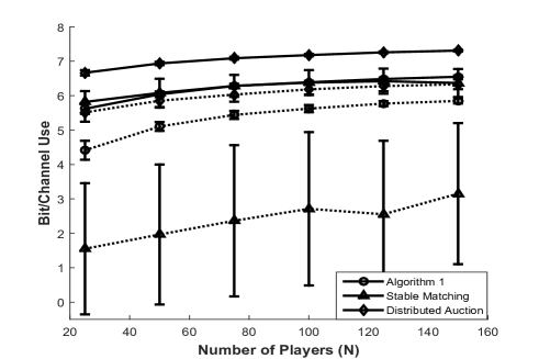
Figure 9: Rates as a function of $N$ averaged over 100 realizations, compared to state of the art algorithms.

VII Conclusion

We used a utility design approach and constructed a non-cooperative game such that all its pure NE have an asymptotically optimal weighted sum-rate. By modifying the fictitious play algorithm for the wireless environment, whose stable points are the pure NE of the designed game, we designed a fully distributed channel allocation algorithm that requires no communication between users. This means we have used game theory as a distributed optimization tool.

Analyzing the performance of the designed game involved a novel probabilistic analysis of the random pure NE of a random interference game in a large network. We defined a bipartite graph of users and resources that represents the $M$ best (or worst) REs of each user. We observed that the random structure of our random NE is an “almost” perfect matching in this random bipartite graph. By taking the number of users ($N$) to infinity, we were able to provide concentration results on the existence (or non-existence) of pure NE in our random game. This novel approach can be applied in other problems, by first identifying the structure of the random NE.

The first game we analyzed is the naive non-cooperative game (Naive-FSIG), where the utility function of each user is simply his achievable rate. We showed that with strong enough interference it has $\varOmega\left(\left(N^{\mu}\right)!\right)$ (for all $\mu<1$) bad pure NE, where $N$ is the number of users.

Then we proposed a designed non-cooperative game formulation (M-FSIG) whose utility is a slight modification of former, such that it is greater than zero only for their $M$ best REs, with the same value for those REs. We proved that asymptotically in $N$, all of its PNE are almost a a perfect matching between users and $M$-best REs (or an exact one) in our bipartite graph. This means that almost all users get one of their $M$ best REs, interference-free.

In order to answer the question of how good is the $M$ best RE, we analyzed the order statistics of the fading distribution. We defined the family of exponentially-dominated tail distributions, that includes many fading distributions (like Rayleigh fading), and showed that for any such distribution the M-FSIG has a pure price of anarchy that converges in probability to 1 as $N\rightarrow\infty$, in any interference regime. Moreover, the M-FSIG exhibits $\varOmega\left(\left(N^{\mu}\right)!\right)$ (for all $\mu<1$) perfect matching pure NE that maintain max-min fairness among the users.

We also proved that the asymptotic optimality of the M-FSIG holds beyond the case of i.i.d. REs. All of our results on the M-FSIG hold for $m$-dependent REs for each user, as appears in practice in OFDMA systems.

For some fixed $N$ the introduced parameter $M$ can be chosen to compromise between sum-rate and fairness. Due to the almost completely orthogonal transmissions in equilibria, our allocation algorithm is more suitable for the medium-strong interference regime.

We showed through simulations that our algorithm converges very fast to the proven pure NE. The fast convergence enables frequent runs of the algorithm in the network, which results in maintaining multi-user diversity in a dynamic fading environment.

Appendix A Proofs for the Naive-FSIG

In this section we provide the proofs of the results in Section IV.

Proof:

Let $\varepsilon>0$. Due to the i.i.d. assumption, the number $N_{\varepsilon,n}$ of r.v. from $\left|h_{n,n,1}\right|,\,...,\,\left|h_{n,n,N}\right|$ that are smaller than $\varepsilon$ has a binomial distribution with $p_{n}=\Pr\left(\left|h_{n,n,1}\right|<\varepsilon\right)>0$. We use the Chernoff-Hoeffding Theorem [60] as a tail bound for $\frac{M_{N}}{N}<p_{n}$. By the assumption on $M_{N}$, $\frac{M_{N}}{N}<p_{n}$ holds for all $N>N_{1}$ for some large enough $N_{1}$, and so

$$\Pr\left(N_{\varepsilon,n}\leq M_{N}\right)\leq\exp\left(-ND\left(\frac{M_{N}}{N}\|p_{n}\right)\right)$$ (16)

where $D(q\|p)=q\ln\frac{q}{p}+\left(1-q\right)\ln\frac{1-q}{1-p}$ , and in our case

$$D\left(\frac{M_{N}}{N}\|p_{n}\right)=\frac{M_{N}}{N}\ln\frac{M_{N}}{Np_{n}}+\left(1-\frac{M_{N}}{N}\right)\ln\frac{1-\frac{M_{N}}{N}}{1-p_{n}}$$ (17)

for which we get by using $\underset{N\rightarrow\infty}{\lim}\frac{M_{N}}{N}=0$ that

$$\underset{N\rightarrow\infty}{\lim}D\left(\frac{M_{N}}{N}\|p_{n}\right)=-\underset{N\rightarrow\infty}{\lim}\frac{\ln\frac{N}{M_{N}}}{\frac{N}{M_{N}}}-\ln p_{n}\underset{N\rightarrow\infty}{\lim}\frac{M_{N}}{N}+\ln\left(\frac{1}{1-p_{n}}\right)\underset{N\rightarrow\infty}{\lim}\left(1-\frac{M_{N}}{N}\right)+\\ \underset{N\rightarrow\infty}{\lim}\left(1-\frac{M_{N}}{N}\right)\ln\left(1-\frac{M_{N}}{N}\right)=\ln\left(\frac{1}{1-p_{n}}\right).$$ (18)

So for large enough $N$ the inequality $D\left(\frac{M_{N}}{N}\|p_{n}\right)\geq\ln\left(\frac{1}{1-p_{n}}\right)-\ln\left(\frac{1}{1-p_{n}^{2}}\right)$ holds; hence we get the following upper bound

$$\Pr\left(N_{\varepsilon,n}\leq M_{N}\right)\leq\exp\left(-ND\left(\frac{M_{N}}{N}\|p_{n}\right)\right)\leq\left(1-p_{n}\right)^{N}\left(\frac{1}{1-p_{n}^{2}}\right)^{N}=\left(\frac{1}{1+p_{n}}\right)^{N}\rightarrow 0.$$ (19)

Clearly, if there are at least $M_{N}$ successes then the $M_{N}$ smallest variables among $\left|h_{n,n,1}\right|,\,...,\,\left|h_{n,n,N}\right|$ are smaller than $\varepsilon$. Consequently, using the union bound we get

$$\underset{N\rightarrow\infty}{\lim}\Pr\left(\underset{n}{\max\,}\left|h_{n,n,(m)}\right|>\varepsilon\right)=\underset{N\rightarrow\infty}{\lim}\Pr\left(\bigcup_{n=1}^{N}\left\{\left|h_{n,n,(m)}\right|>\varepsilon\right\}\right)\leq\underset{N\rightarrow\infty}{\lim}\sum_{n=1}^{N}\frac{1}{\left(1+p_{n}\right)^{N}}=0$$ (20)

for each $m\leq M_{N}$ and each $\varepsilon>0$, and we reach our conclusion. ∎

Appendix B Exponentially-Dominated Tail Distributions

Our order statistics analysis provided in Appendix C is valid for a broad family of fading distributions, named exponentially-dominated tail distributions (see Definition V.2). In this appendix we develop the properties of these distributions that are essential for our results.

The Rayleigh, Rician, m-Nakagami and Normal distributions all have an exponentially-dominated tail. To ease the verification that a certain distribution has an exponentially-dominated tail, we provide the following lemma. The conditions of this lemma are easier to check than Definition V.2 where the PDF has a more convenient form than the CDF, or when a certain power of the original random variable has a more convenient distribution.

Lemma B.1.

Let $X$ be a positive random variable with a CDF $F_{X}$ and a PDF $f_{X}$.

1. If for some $\alpha,\gamma,\lambda>0$ and $\beta\in\mathbb{R}$, $\underset{x\rightarrow\infty}{\lim}\frac{f_{X}\left(x\right)}{\alpha\gamma\lambda x^{\beta+\gamma-1}e^{-\lambda x^{\gamma}}}=1$ holds then $X$ has an exponentially-dominated tail distribution.

2. For any $d>0$, if $X$ has an exponentially-dominated tail distribution then so does $X^{d}$.

Proof:

The first part follows from l’H pital’s rule

$$\underset{x\rightarrow\infty}{\lim}\frac{1-F_{X}\left(x\right)}{\alpha x^{\beta}e^{-\lambda x^{\gamma}}}=\underset{x\rightarrow\infty}{\lim}\frac{-f_{X}\left(x\right)}{-\alpha\gamma\lambda x^{\beta+\gamma-1}e^{-\lambda x^{\gamma}}+\alpha\beta x^{\beta-1}e^{-\lambda x^{\gamma}}}=\underset{x\rightarrow\infty}{\lim}\frac{\frac{f_{X}\left(x\right)}{\alpha\gamma\lambda x^{\beta+\gamma-1}e^{-\lambda x^{\gamma}}}}{1-\frac{\beta}{\gamma\lambda x^{\gamma}}}=1.$$ (21)

For the second part, note that if $Y=X^{d}$ then $F_{Y}\left(y\right)=F_{X}\left(y^{1/d}\right)$; hence $\underset{y\rightarrow\infty}{\lim}\frac{1-F_{Y}\left(y\right)}{\alpha y^{\frac{\beta}{d}}e^{-\lambda y^{\frac{\gamma}{d}}}}=\underset{y\rightarrow\infty}{\lim}\frac{1-F_{X}\left(y^{1/d}\right)}{\alpha\left(y^{1/d}\right)^{\beta}e^{-\lambda\left(y^{1/d}\right)^{\gamma}}}=1$. ∎

Note that the second part of the above lemma allows us to choose our $X_{n,k}$ variable in Section V.I as either $\frac{1}{a_{n}}|h_{n,n,k}|^{2}$ or $\frac{1}{\sqrt{a_{n}}}$$|h_{n,n,k}|$, where $a_{n}=E\left\{|h_{n,n,k}|^{2}\right\}$ for all $k$.

Due to our interest in the intermediate statistics compared to the extreme statistics, the desired properties of exponentially-dominated tail distributions will be expressed by the quantile function. The following definition will simplify notations.

Definition B.2.

Define the tail quantile function as $\bar{q}_{X}\left(p\right)=F_{X}^{-1}\left(1-p\right)=\min\left\{x\,|\,F_{X}\left(x\right)\geq 1-p\right\}$.

The next proposition lists important properties of exponentially-dominated tail distributions we will need for our proofs. These properties are regrading the quantile function of an exponentially-dominated tail distribution, and its intermediate to extreme statistics ratio.

Proposition B.3.

Let $X$ be a random variable with a tail quantile function $\bar{q}_{X}\left(p\right)$ . If $X$ has an exponentially-dominated tail distribution with parameters $\alpha,\gamma,\lambda>0$ and $\beta\in\mathbb{R}$, then

1. $\underset{p\rightarrow 0}{\lim}\frac{\bar{q}_{X}\left(p\right)}{\left[\frac{1}{\lambda}\ln\left(\alpha\frac{1}{p}\right)\right]^{1/\gamma}}=1$.

2. If $\underset{K\rightarrow\infty}{\lim}\frac{M_{K}}{\ln^{\mu}K}=0$ for some $\mu>0$ then $\underset{K\rightarrow\infty}{\lim}\frac{\bar{q}_{X}\left(\frac{M_{K}}{K}\right)}{\bar{q}_{X}\left(\frac{1}{K}\right)}=1$.

3. If $\underset{K\rightarrow\infty}{\lim}\frac{M_{K}}{K^{\mu}}=0$ for some $\mu<1$ then $\underset{K\rightarrow\infty}{\lim}\frac{\bar{q}_{X}\left(\frac{M_{K}}{K}\right)}{\bar{q}_{X}\left(\frac{1}{K^{2}}\right)}>0$.

Proof:

Define $g_{1}\left(x\right)=\alpha e^{-\lambda\left(x^{\gamma}+2x^{\gamma/2}\right)}$, $g_{2}\left(x\right)=\alpha e^{-\lambda\left(x^{\gamma}-2x^{\gamma/2}\right)}$. Let $\varepsilon>0$. For some large enough $x_{1}>0$, the inequality

$$\frac{1}{1-\varepsilon}\alpha e^{-\lambda\left(x^{\gamma}+2x^{\gamma/2}\right)}\leq\alpha x^{\beta}e^{-\lambda x^{\gamma}}\leq\frac{1}{1+\varepsilon}\alpha e^{-\lambda\left(x^{\gamma}-2x^{\gamma/2}\right)}$$ (22)

holds for all $x>x_{1}$. Due to the exponentially-dominated tail, for some large enough $x_{2}>0$, the inequality

$$\left(1-\varepsilon\right)\alpha x^{\beta}e^{-\lambda x^{\gamma}}\leq 1-F_{X}\left(x\right)\leq\left(1+\varepsilon\right)\alpha x^{\beta}e^{-\lambda x^{\gamma}}$$ (23)

holds for all $x>x_{2}$. Combining (22) and (23) we conclude that for all $x>\max\left\{x_{1},x_{2}\right\}$ the following inequality holds

$$g_{1}\left(x\right)=\alpha e^{-\lambda\left(x^{\gamma}+2x^{\gamma/2}\right)}\leq 1-F_{X}\left(x\right)\leq\alpha e^{-\lambda\left(x^{\gamma}-2x^{\gamma/2}\right)}=g_{2}\left(x\right).$$ (24)

For small enough $p$, the tail quantile function $\bar{q}_{X}\left(p\right)$ is large enough, i.e., $\bar{q}_{X}\left(p\right)>\max\left\{x_{1},x_{2}\right\}$ and from (24) we get

$$\begin{array}[]{c}g_{1}\left(\bar{q}_{X}\left(p\right)\right)\leq p=1-F_{X}\left(\bar{q}_{X}\left(p\right)\right)\leq g_{2}\left(\bar{q}_{X}\left(p\right)\right)\end{array}.$$ (25)

It is easy to verify that for $p\leq\alpha$, such that $\ln\left(\frac{\alpha}{p}\right)\geq 0$, we have

$$\begin{array}[]{c}g_{1}^{-1}\left(p\right)=\left[\sqrt{\frac{1}{\lambda}\ln\left(\frac{\alpha}{p}\right)+1}-1\right]^{2/\gamma}\\ \\ g_{2}^{-1}\left(p\right)=\left[\sqrt{\frac{1}{\lambda}\ln\left(\frac{\alpha}{p}\right)+1}+1\right]^{2/\gamma}\end{array}.$$ (26)

Hence by invoking $g_{1}^{-1}\left(p\right),g_{2}^{-1}\left(p\right)$, which are monotonically decreasing, on the first and second inequalities in (25) respectively, we get that for small enough $p$ the following holds

$$\left[\sqrt{\frac{1}{\lambda}\ln\left(\frac{\alpha}{p}\right)+1}-1\right]^{2/\gamma}\leq\bar{q}_{X}\left(p\right)\leq\left[\sqrt{\frac{1}{\lambda}\ln\left(\frac{\alpha}{p}\right)+1}+1\right]^{2/\gamma}$$ (27)

which leads to

$$\underset{p\rightarrow 0}{\lim}\frac{\bar{q}_{X}\left(p\right)}{\left[\frac{1}{\lambda}\ln\left(\frac{\alpha}{p}\right)\right]^{1/\gamma}}\geq\underset{p\rightarrow 0}{\lim}\frac{\left[\sqrt{\frac{1}{\lambda}\ln\left(\frac{\alpha}{p}\right)+1}-1\right]^{2/\gamma}}{\left[\frac{1}{\lambda}\ln\left(\frac{\alpha}{p}\right)\right]^{1/\gamma}}=1$$ (28)

and

$$\underset{p\rightarrow 0}{\lim}\frac{\bar{q}_{X}\left(p\right)}{\left[\frac{1}{\lambda}\ln\left(\frac{\alpha}{p}\right)\right]^{1/\gamma}}\leq\underset{p\rightarrow 0}{\lim}\frac{\left[\sqrt{\frac{1}{\lambda}\ln\left(\frac{\alpha}{p}\right)+1}+1\right]^{2/\gamma}}{\left[\frac{1}{\lambda}\ln\left(\frac{\alpha}{p}\right)\right]^{1/\gamma}}=1$$ (29)

where both limits stem from $\left[\frac{1}{\lambda}\ln\left(\frac{\alpha}{p}\right)\right]^{1/\gamma}$ being the dominant term in $\left[\sqrt{\frac{1}{\lambda}\ln\left(\frac{\alpha}{p}\right)+1}\pm 1\right]^{2/\gamma}$. Together (28) and (29) yield $\underset{p\rightarrow 0}{\lim}\frac{\bar{q}_{X}\left(p\right)}{\left[\frac{1}{\lambda}\ln\left(\frac{\alpha}{p}\right)\right]^{1/\gamma}}=1$. Now let $M_{K}$ be a sequence such that $\underset{K\rightarrow\infty}{\lim}\frac{M_{K}}{\ln^{\mu}K}=0$ for some $\mu>0$ and obtain

$$\underset{K\rightarrow\infty}{\lim}\frac{\bar{q}_{X}\left(\frac{M_{K}}{K}\right)}{\bar{q}_{X}\left(\frac{1}{K}\right)}\underset{(a)}{=}\underset{K\rightarrow\infty}{\lim}\frac{\bar{q}_{X}\left(\frac{M_{K}}{K}\right)}{\left[\frac{1}{\lambda}\ln\left(\alpha\frac{K}{M_{K}}\right)\right]^{1/\gamma}}\underset{K\rightarrow\infty}{\lim}\frac{\left[\frac{1}{\lambda}\ln\left(\alpha K\right)\right]^{1/\gamma}}{\bar{q}_{X}\left(\frac{1}{K}\right)}\underset{(b)}{=}1$$ (30)

where (a) follows from $\underset{K\rightarrow\infty}{\lim}\frac{\left[\frac{1}{\lambda}\ln\left(\alpha K\right)\right]^{1/\gamma}}{\left[\frac{1}{\lambda}\ln\left(\alpha\frac{K}{M_{K}}\right)\right]^{1/\gamma}}=1$, which is true due to $\underset{K\rightarrow\infty}{\lim}\frac{M_{K}}{\ln^{\mu}K}=0$ for some $\mu>0$, and (b) from Part 1. Now let $M_{K}$ be a sequence such that $\underset{K\rightarrow\infty}{\lim}\frac{M_{K}}{K^{\mu}}=0$ for some $\mu<1$ and obtain

$$\underset{K\rightarrow\infty}{\lim}\frac{\bar{q}_{X}\left(\frac{M_{K}}{K}\right)}{\bar{q}_{X}\left(\frac{1}{K^{2}}\right)}\underset{(a)}{=}\underset{K\rightarrow\infty}{\lim}\frac{\left[\frac{1}{\lambda}\ln\left(\alpha\frac{K}{M_{K}}\right)\right]^{1/\gamma}}{\left[\frac{1}{\lambda}\ln\left(\alpha K^{2}\right)\right]^{1/\gamma}}=\left(\frac{1}{2}\right)^{1/\gamma}\underset{K\rightarrow\infty}{\lim}\left(\frac{\ln\left(\alpha\frac{K}{M_{K}}\right)}{\ln\left(\sqrt{\alpha}K\right)}\right)^{1/\gamma}\underset{(b)}{>}0$$ (31)

where (a) follows from $\underset{K\rightarrow\infty}{\lim}\frac{\bar{q}_{X}\left(\frac{M_{K}}{K}\right)}{\left[\frac{1}{\lambda}\ln\left(\alpha\frac{K}{M_{K}}\right)\right]^{1/\gamma}}=1$ and $\underset{K\rightarrow\infty}{\lim}\frac{\bar{q}_{X}\left(\frac{1}{K^{2}}\right)}{\left[\frac{1}{\lambda}\ln\left(\alpha K^{2}\right)\right]^{1/\gamma}}=1$, which we proved in Part 1, and (b) from the assumption that $\underset{K\rightarrow\infty}{\lim}\frac{M_{K}}{K^{\mu}}=0$ for some $\mu<1$. ∎

It should be emphasized that, technically speaking, the only result in this paper that actually requires the exponentially-dominated tail assumption is Proposition B.3 above. Also note that Parts 2 and 3 of this Proposition follow from Part 1 directly. Therefore, all our order statistics analysis automatically applies to any distribution $F_{X}\left(x\right)$ with a tail quantile function $\bar{q}_{X}\left(p\right)$ such that $\underset{p\rightarrow 0}{\lim}\frac{\bar{q}_{X}\left(p\right)}{\left[\frac{1}{\lambda}\ln\left(\alpha\frac{1}{p}\right)\right]^{1/\gamma}}=1$. The question of how broader this class than the family of exponentially-dominated tail distributions remains open.

Appendix C Proofs for the M-FSIG

In this section we provide the proofs of the results in Section V.

C-A Proof of Theorem V.6

Proof:

Denote the number of shared REs by $K_{c}$. Denote the number of sharing users by $N_{c}$. In each shared RE, every user except one contributes one empty RE to the total number of empty REs $E$, so $E=N_{c}-K_{c}$. Every shared RE must contain at least two users; hence $\frac{N_{c}}{2}\leq E\leq N_{c}$. In a PNE for the M-FSIG, no empty RE can be one of the $M$- best REs of one of the sharing users.

Let $\mathcal{E}$ be a set of empty REs with cardinality $E$ and $\mathcal{S}$ be a set of sharing users with cardinality $N_{c}$. We want to upper bound the probability that user $n$ will not have any of the $E$ empty REs in $\mathcal{E}$ in his $M$-best RE list. For i.i.d. channel gains this can be done as follows

$$\Pr\left(\mathcal{M}_{n}\cap\mathcal{E}=\emptyset\right)\underset{(a)}{=}\frac{\left(\begin{array}[]{c}K-E\\ M\end{array}\right)}{\left(\begin{array}[]{c}K\\ M\end{array}\right)}=\frac{(K-E)!(K-M)!}{K!(K-E-M)!}=\prod_{i=1}^{E}\frac{K-E-M+i}{K-E+i}=\\ \prod_{i=1}^{E}\left(1-\frac{M}{K-E+i}\right)\underset{(b)}{\leq}\left(1-\frac{M}{K}\right)^{E}\underset{(c)}{\leq}e^{-M\frac{E}{K}}\underset{(d)}{\leq}e^{-M\frac{N_{c}}{2K}}$$ (32)

where (a) follows from $h_{n,n,1},\,...,\,h_{n,n,k}$ being i.i.d., (b) follows from $1-\frac{M}{K-E+i}\leq 1-\frac{M}{K}$ for $i=1,...,E$, (c) from $\left(1-\frac{M}{K}\right)^{K}\leq e^{-M}$ and (d) from $E\geq\frac{N_{c}}{2}$. For the $m$-dependent case we have instead, from Lemma D.1 that

$$\Pr\left(\mathcal{M}_{n}\cap\mathcal{E}=\emptyset\right)\leq\left(m+1\right)e^{-\frac{M}{e\left(m+1\right)}\frac{N-m-1}{N+m+1}}+\left(1-\frac{M}{e\left(N+m+1\right)}\right)^{\frac{E}{m+1}}\underset{(a)}{\leq}\\ \left(m+1\right)e^{-\frac{M}{e\left(m+1\right)}\frac{N-m-1}{N+m+1}}+e^{-\frac{M}{e\left(m+1\right)}\frac{E}{N+m+1}}\underset{(b)}{\leq}\left(m+2\right)e^{-\frac{M}{e\left(m+1\right)}\frac{E}{N+m+1}}$$ (33)

where (a) is from $\left(1-\frac{x}{L}\right)^{L}\leq e^{-x}$ which is true for each $x<L$ where $L$ is a positive integer, and (b) by comparing the exponents for $E\leq N-m-1$. Denote by $\mathcal{E_{\mathbf{a}}}$ and $\mathcal{S_{\mathbf{a}}}$ the set of empty REs and the set of sharing users, respectively, of the strategy profile $\mathbf{a}$. We get, using (33), that

$$\Pr\left(\left\{\mathbf{a}\,|\,\mathcal{\mathcal{E}\,\subseteq E_{\mathbf{a}}},\,\mathcal{S\subseteq S_{\mathbf{a}}}\right\}\cap\mathcal{P}_{e}\neq\emptyset\right)\underset{(a)}{\leq}\\ \Pr\left(\bigcap_{n\in\mathcal{S}}\left\{\mathcal{M}_{n}\cap\mathcal{E}=\emptyset\right\}\right)\underset{(b)}{=}\bigcap_{n\in\mathcal{S}}\Pr\left(\mathcal{M}_{n}\cap\mathcal{E}=\emptyset\right)\underset{(c)}{\leq}\left(m+2\right)^{N_{c}}e^{-\frac{M}{2e\left(m+1\right)}\frac{N_{c}^{2}}{N+m+1}}$$ (34)

where (a) is because $\left\{\mathbf{a}\,|\,\mathcal{\mathcal{E}\,\subseteq E_{\mathbf{a}}},\,\mathcal{S\subseteq S_{\mathbf{a}}}\right\}\cap\mathcal{P}_{e}\neq\emptyset$ implies $\bigcap_{n\in\mathcal{S}}\left\{\mathcal{M}_{n}\cap\mathcal{E}=\emptyset\right\}$, (b) is due to the independence of users’ preferences, and (c) from (33). This means that the set of all the strategy profiles with empty REs and sharing users sets that contain $\mathcal{E}$ and $\mathcal{S}$, respectively, have a vanishing probability to contain a PNE, if $N_{c}=rN$ for some $0<r<1$. Now we want to show that even$\underset{\mathbf{a^{*}}\in\mathcal{P}_{e}}{\max}\frac{N_{c}\left(\mathbf{a^{*}}\right)}{N}\rightarrow 0$ as $N\rightarrow\infty$. We want to find a probabilistic upper bound $\tilde{N_{c}}$ for the number of sharing users that a PNE may contain. We use the union bound over all the choices of $\tilde{N_{c}}$ sharing users and the set of $\tilde{E}=\frac{\tilde{N_{c}}}{2}$ necessarily existing empty REs, to get from (34) that

$$\Pr\left(\underset{\mathbf{a^{*}}\in\mathcal{P}_{e}}{\max}N_{c}\left(\mathbf{a^{*}}\right)\geq\tilde{N_{c}}\right)\underset{(a)}{=}\Pr\left(\left\{\mathbf{a}\,|\,\left|\mathcal{S_{\mathbf{a}}}\right|\geq\tilde{N_{c}}\,,\,\left|\mathcal{E_{\mathbf{a}}}\right|\geq\tilde{E}\right\}\cap\mathcal{P}_{e}\neq\emptyset\right)\underset{(b)}{=}\\ \Pr\left(\bigcup_{\mathcal{\mathit{\mathcal{S},\mathcal{E}\in\Lambda}}}\biggl{\{}\left\{\mathbf{a}\,|\,\mathcal{\mathcal{E}\,\subseteq E_{\mathbf{a}}},\,\mathcal{S\subseteq S_{\mathbf{a}}}\right\}\cap\mathcal{P}_{e}\neq\emptyset\biggr{\}}\right)\underset{(c)}{\leq}\left(\begin{array}[]{c}N\\ \tilde{N_{c}}\end{array}\right)\left(\begin{array}[]{c}K\\ \tilde{E}\end{array}\right)\left(m+2\right)^{\tilde{N_{c}}}e^{-\frac{M}{2e\left(m+1\right)}\frac{\tilde{N_{c}}^{2}}{N+m+1}}.$$ (35)

The event $\underset{\mathbf{a^{*}}\in\mathcal{P}_{e}}{\max}N_{c}\left(\mathbf{a^{*}}\right)\geq\tilde{N_{c}}$ occurs if and only if some PNE has at least $\tilde{N_{c}}$ sharing users. This is used in (a). Equality (b) follows from going over all the options in $\Lambda=\left\{\mathcal{S},\mathcal{E}\,|\,\left|\mathcal{S}\right|=\tilde{N_{c}},\left|\mathcal{E}\right|=\tilde{E}\right\}$, and (c) is the union bound. The inequality in (35) bounds the probability that there exists a PNE with at least $\tilde{N_{c}}$ sharing users. Now choose $\tilde{N_{c}}=rN$ for some $0<r\leq\frac{1}{2}$ , so $\left(\begin{array}[]{c}K\\ \tilde{E}\end{array}\right)\leq\left(\begin{array}[]{c}N\\ \tilde{N_{c}}\end{array}\right)$. We can use the bound $\left(\begin{array}[]{c}N\\ rN\end{array}\right)\leq\sqrt{\frac{1}{2\pi r\left(1-r\right)N}}2^{Nh_{2}\left(r\right)}$ [61] where $h_{2}(r)$ is the binary entropy of $r$ and obtain from (35) that

$$\Pr\left(\underset{\mathbf{a^{*}}\in\mathcal{P}_{e}}{\max}N_{c}\left(\mathbf{a^{*}}\right)\geq rN\right)\leq\frac{\left(m+2\right)^{rN}}{2\pi r\left(1-r\right)N}4^{Nh_{2}(r)}e^{-\frac{M}{2e\left(m+1\right)}\frac{N}{N+m+1}r^{2}N}\underset{(a)}{\leq}\\ \frac{1}{2\pi r\left(1-r\right)N}\left(\frac{\left(m+2\right)^{r}4^{h_{2}(r)}}{e^{\frac{r^{2}}{6\left(m+1\right)}M}}\right)^{N}\underset{(b)}{\leq}\frac{1}{2\pi r\left(1-r\right)N}\left(\frac{\left(m+2\right)^{r}4^{h_{2}(r)}}{N^{r^{2}\frac{\varepsilon+e}{6}}}\right)^{N}$$ (36)

where (a) is due to $\frac{N}{N+m+1}\geq\frac{2e}{6}$ for large enough $N$ and (b) follows from $M\geq\left(e+\varepsilon\right)\left(m+1\right)\ln(N)$. In conclusion we get that $\underset{N\rightarrow\infty}{\lim}\Pr\left(\underset{\mathbf{a^{*}}\in\mathcal{P}_{e}}{\max}\frac{N_{c}\left(\mathbf{a^{*}}\right)}{N}<r\right)=1$ for all $r>0$ and hence $\underset{\mathbf{a^{*}}\in\mathcal{P}_{e}}{\max}\frac{N_{c}\left(\mathbf{a^{*}}\right)}{N}\rightarrow 0$ in probability as $N\rightarrow\infty$.

Note that substituting $m=0$ in (36) yields a slightly looser bound than we can get with a direct analysis of i.i.d. channel gains. With i.i.d. channel gains, the factor $\left(m+2\right)^{r}$ disappears and $N^{r^{2}\frac{\varepsilon+e}{6}}$ is replaced by $N^{r^{2}\frac{\varepsilon+e}{2}}$. This is easily verified using (32) instead of (33). ∎

C-B Proofs of Theorem V.9 and Theorem V.11

In order to prove Theorem V.9, we need the following two lemmas that provide probabilistic bounds on the relevant random variables.

The first is a probabilistic upper bound for the extreme statistics of an exponentially-dominated tail distribution. Note that this lemma assumes nothing regrading the independence of the series of random variables.

Lemma C.1.

Let $\left\{X_{n,k}\right\}$ be identically distributed unbounded random variables with exponentially-dominated tail distribution $F_{X}$ with parameters $\alpha,\gamma,\lambda>0$ and $\beta\in\mathbb{R}$. If $U_{K}=\left(\frac{\ln\left(K\right)+\sqrt{\ln\left(K\right)}}{\lambda}\right)^{1/\gamma}$ then

1. $\underset{K\rightarrow\infty}{\lim}\Pr\left(X_{n,(K)}\leq U_{K}\right)=1$ for each $n\in\mathcal{N}$.

2. $\underset{N\rightarrow\infty}{\lim}\Pr\left(\underset{n}{\max\,}X_{n,(K)}\leq U_{N^{2}}\right)=1$.

Proof:

From the union bound and the identical distributions of $X_{n,1},...,X_{n,K}$ we obtain

$$\Pr\left(X_{n,(K)}\geq U_{K}\right)=\Pr\left(\bigcup_{k=1}^{K}\left\{X_{n,k}\geq U_{K}\right\}\right)\leq K\Pr\left(X_{n,1}\geq U_{K}\right).$$ (37)

We get that for $U_{K}=\left(\frac{\ln\left(K\right)+\sqrt{\ln\left(K\right)}}{\lambda}\right)^{1/\gamma}$

$$\underset{K\rightarrow\infty}{\lim}K\Pr\left(X_{n,1}\geq U_{K}\right)=\underset{K\rightarrow\infty}{\lim}\frac{\Pr\left(X_{n,1}\geq U_{K}\right)}{\alpha U_{K}^{\beta}e^{-\lambda U_{K}^{\gamma}}}\underset{K\rightarrow\infty}{\lim}\frac{\alpha U_{K}^{\beta}K}{\exp\left(\ln\left(K\right)+\sqrt{\ln\left(K\right)}\right)}\underset{(a)}{=}\\ \frac{\alpha}{\lambda^{\beta/\gamma}}\underset{K\rightarrow\infty}{\lim}\left(\ln\left(K\right)+\sqrt{\ln\left(K\right)}\right)^{\beta/\gamma}\exp\left(-\sqrt{\ln\left(K\right)}\right)=0$$ (38)

where (a) is from the definition of an exponentially-dominated tail. This proves the first part of the lemma. For the second part consider all the variables $\left\{X_{n,k}\right\}$, as $NK=N^{2}$ identically distributed samples from the parent distribution $F_{X}\left(x\right)$, and define $X_{(N^{2})}=\underset{n}{\max\,}X_{n,(K)}$. By substituting $K=N^{2}$ in the derivation above the result readily follows. ∎

Next we prove the probabilistic lower bound for the intermediate statistics of an exponentially-dominated tail distribution. Note that the next lemma holds for m-dependent sequences of random variables.

Lemma C.2.

Let $\left\{X_{n,k}\right\}$ be identically distributed unbounded random variables with an exponentially-dominated tail distribution $F_{X}$. Assume that $\left\{X_{n,k}\right\}_{k}$ is $m$-dependent for each $n$. Let $M_{K}$ be a sequence such that $\underset{K\rightarrow\infty}{\lim}\frac{M_{K}}{K}=0$ and $\underset{K\rightarrow\infty}{\lim}M_{K}=\infty$ and define $L_{K}=F_{X}^{-1}\left(1-\frac{e^{2}M_{K}}{K}\right)$. If $M_{K}\geq\left(m+1\right)(1+\varepsilon)\ln K$ for some $\varepsilon>0$ then

1. For large enough $K$ we have $\Pr\left(X_{n,(K-M_{K}+1)}\geq L_{K}\right)\geq 1-\frac{2\left(m+1\right)}{K^{4(1+\varepsilon)}}$ for each $n\in\mathcal{N}$.

2. $\underset{K\rightarrow\infty}{\lim}\Pr\left(\underset{n}{\min}\,X_{n,(K-M_{K}+1)}\geq L_{K}\right)=1$.

Proof:

Let $L_{K}=\bar{q}_{X}\left(\frac{e^{2}M_{K}}{K}\right)$. By invoking $F_{K}\left(x\right)=\sum_{k=1}^{K}I\left(X_{n,k}\leq x\right)$ on both sides of $X_{n,(K-M_{K}+1)}\leq L_{K}$ we get

$$\Pr\left(X_{n,(K-M_{K}+1)}\leq L_{K}\right)=\Pr\left(K-M_{K}+1\leq\sum_{k=1}^{K}I\left(X_{n,k}\leq L_{K}\right)\right)\underset{(a)}{=}\Pr\left(\sum_{k=1}^{K}I\left(X_{n,k}>L_{K}\right)<M_{K}\right)$$ (39)

where (a) follows by $K-\sum_{k=1}^{K}I\left(X_{n,k}\leq L_{K}\right)=\sum_{k=1}^{K}I\left(X_{n,k}>L_{K}\right)$. Now we divide $X_{n,1},...,X_{n,K}$ into $m+1$ disjoint sets $\left\{X_{n,1},X_{n,2+m},...\right\},...,\left\{X_{n,m+1},X_{n,2+2m},...\right\}$ and define $Y_{n,i,j}=X_{n,j+\left(m+1\right)i}$ for $j=1,..,m+1$ and all $i$ such that $1\leq j+\left(m+1\right)i\leq K$ for some $j$. Note that there are $\left\lfloor\frac{K}{m+1}\right\rfloor+1$ or $\left\lfloor\frac{K}{m+1}\right\rfloor$ elements in each of these sets. By omitting the last element in the larger sets we obtain

$$\sum_{k=1}^{K}I\left(X_{n,k}>L_{K}\right)\geq\sum_{j=1}^{m+1}\sum_{i=0}^{\left\lfloor\frac{K}{m+1}\right\rfloor-1}I\left(X_{n,j+\left(m+1\right)i}>L_{K}\right)=\sum_{j=1}^{m+1}\sum_{i=0}^{\left\lfloor\frac{K}{m+1}\right\rfloor-1}I\left(Y_{n,i,j}>L_{K}\right).$$ (40)

Because $X_{n,1},...,X_{n,K}$, are $m$-dependent, $Y_{n,0,j},...,Y_{n,\left\lfloor\frac{K}{m+1}\right\rfloor-1,j}$ are independent random variables for each $j$. For large enough $K$, $\frac{\left(m+1\right)M_{K}}{K}<1$ and so

$$\Pr\left(\sum_{k=1}^{K}I\left(X_{n,k}>L_{K}\right)<M_{K}\right)=\Pr\left(\sum_{k=1}^{K}I\left(X_{n,k}>L_{K}\right)<M_{K}-\frac{\left(m+1\right)M_{K}}{K}\right)$$ (41)

since $\sum_{k=1}^{K}I\left(X_{n,k}>L_{K}\right)$ is an integer. Denote $t=\left(m+1\right)\frac{M_{K}}{K}\left\lfloor\frac{K}{m+1}\right\rfloor$ and note that $M_{K}-\frac{\left(m+1\right)M_{K}}{K}\leq t\leq M_{K}$. By the union bound and the identical distributions of $\left\{X_{n,k}\right\}$ we get, for large enough $K$, that

$$\Pr\left(\sum_{k=1}^{K}I\left(X_{n,k}>L_{K}\right)<M_{K}\right)\underset{(a)}{=}\Pr\left(\sum_{k=1}^{K}I\left(X_{n,k}>L_{K}\right)<t\right)\underset{(b)}{\leq}\Pr\left(\sum_{j=1}^{m+1}\sum_{i=0}^{\left\lfloor\frac{K}{m+1}\right\rfloor-1}I\left(Y_{n,i,j}>L_{K}\right)<t\right)\underset{(c)}{\leq}\\ \Pr\left(\bigcup_{j=1}^{m+1}\left\{\sum_{i=0}^{\left\lfloor\frac{K}{m+1}\right\rfloor-1}I\left(Y_{n,i,j}\geq L_{K}\right)<\frac{t}{m+1}\right\}\right)\underset{(d)}{\leq}\left(m+1\right)\Pr\left(\sum_{i=0}^{\left\lfloor\frac{K}{m+1}\right\rfloor-1}I\left(Y_{n,i,1}>L_{K}\right)<\frac{t}{m+1}\right)$$ (42)

where (a) follows from (41), (b) from (40), (c) because some inner sum must be smaller than $\frac{t}{m+1}$ for the total sum to be smaller than $t$ and (d) from the union bound. Define the random variables $Z_{i}=I\left(Y_{n,i,1}\geq L_{K}\right)$ for $i=0,..,\left\lfloor\frac{K}{m+1}\right\rfloor-1$. Due to the independence of $Y_{n,0,j},...,Y_{n,\left\lfloor\frac{K}{m+1}\right\rfloor-1,j}$, these variables form a Bernoulli process with success probability $p=1-F_{X}\left(L_{K}\right)=\frac{e^{2}M_{K}}{K}$. Now we can apply a concentration upper bound on the last term using a Chernoff bound for a Binomially distributed variable. Because $p>\frac{M_{K}}{K}$ we obtain, after substituting $t=\left(m+1\right)\frac{M_{K}}{K}\left\lfloor\frac{K}{m+1}\right\rfloor$, that

$$\Pr\left(\sum_{i=0}^{\left\lfloor\frac{K}{m+1}\right\rfloor-1}I\left(Y_{n,i,1}>L_{K}\right)<\frac{\left(m+1\right)\frac{M_{K}}{K}\left\lfloor\frac{K}{m+1}\right\rfloor}{m+1}\right)\leq\\ \exp\left(-\left\lfloor\frac{K}{m+1}\right\rfloor D\left(\frac{M_{K}}{K}||p\right)\right)$$ (43)

and for large enough $K$

$$D\left(\frac{M_{K}}{K}||\frac{e^{2}M_{K}}{K}\right)=-\frac{M_{K}}{K}\ln\left(e^{2}\right)+\left(1-\frac{M_{K}}{K}\right)\ln\left(1+\frac{\left(e^{2}-1\right)\frac{M_{K}}{K}}{1-\frac{e^{2}M_{K}}{K}}\right)\underset{(a)}{\geq}-\frac{2M_{K}}{K}+\frac{1-\frac{M_{K}}{K}}{1-\frac{e^{2}M_{K}}{K}}\frac{6M_{K}}{K}\underset{(b)}{\geq}\frac{4M_{K}}{K}$$ (44)

where (a) follows from $\ln\left(1+x\right)\geq\frac{6}{e^{2}-1}x$ for all $x\leq\frac{1}{100}$ together with $\underset{K\rightarrow\infty}{\lim}\frac{M_{K}}{K}=0$ and (b) follows from $\frac{1-\frac{M_{K}}{K}}{1-\frac{e^{2}M_{K}}{K}}\geq 1$. So for large enough $K$ the inequality $D\left(\frac{M_{K}}{K}||\frac{e^{2}M_{K}}{K}\right)\geq\frac{4M_{K}}{K}$ holds. If $M_{K}\geq\left(m+1\right)(1+\varepsilon)\ln\left(K\right)$ for some $\varepsilon>0$ then, we conclude from (39), (42), (43) and (44) that for large enough $K$

$$\Pr\left(X_{n,(K-M_{K}+1)}\leq L_{K}\right)\leq\left(m+1\right)\exp\left(-\left\lfloor\frac{K}{m+1}\right\rfloor D\left(\frac{M_{K}}{K}||\frac{e^{2}M_{K}}{K}\right)\right)\leq\\ \left(m+1\right)\exp\left(-4\left(\frac{M_{K}}{m+1}-\frac{M_{K}}{K}\right)\right)\leq\frac{2\left(m+1\right)}{K^{4(1+\varepsilon)}}$$ (45)

which proves part one, and readily follows to part two by

$$\Pr\left(\underset{n}{\min}\,X_{n,(K-M_{K}+1)}\geq L_{K}\right)=\Pr\left(\bigcap_{n}\left\{X_{n,(K-M_{K}+1)}\geq L_{K}\right\}\right)\underset{(a)}{\geq}\\ N\left(1-\frac{2\left(m+1\right)}{K^{4(1+\varepsilon)}}\right)-(N-1)\underset{(b)}{=}1-\frac{2\left(m+1\right)}{K^{3+4\varepsilon}}\underset{K\rightarrow\infty}{\rightarrow}1$$ (46)

where (a) is from Fr chet inequality and (45) and (b) due to $N=K$. ∎

Using the above lemmas, we can now prove both Theorem V.9 and Theorem V.11.

Proof:

Define $U_{K}=\left(\frac{\ln\left(K\right)+\sqrt{\ln\left(K\right)}}{\lambda}\right)^{1/\gamma}$ and $L_{K}=\overline{q}_{X}\left(\frac{e^{2}M_{K}}{K}\right)$ (see Definition B.2). We get the following inequality

$$\Pr\left(\frac{X_{(K-M_{K}+1)}}{X_{(K)}}\geq\frac{L_{K}}{U_{K}}\right)\underset{(a)}{\geq}\Pr\left(X_{(K-M_{K}+1)}\geq L_{K}\,,\,X_{(K)}\leq U_{K}\right)\underset{(b)}{\geq}\\ 1-\Pr\left(X_{(K-M_{K}+1)}\leq L_{K}\right)-\Pr\left(X_{(K)}\geq U_{K}\right)$$ (47)

where (a) is due to $\left\{X_{(K-M_{K}+1)}\geq L_{K},X_{(K)}\leq U_{K}\right\}\subseteq\left\{\frac{X_{(K-M_{K}+1)}}{X_{(K)}}\geq\frac{L_{K}}{U_{K}}\right\}$ and (b) is the union bound. From Lemma C.1 Part 1 and Lemma C.2 Part 1 we get $\underset{K\rightarrow\infty}{\lim}\Pr\left(\frac{X_{(K-M_{K}+1)}}{X_{(K)}}\geq\frac{L_{K}}{U_{K}}\right)=1$. From Proposition B.3 (Parts 1 and 2)

$$\underset{K\rightarrow\infty}{\lim}\frac{L_{K}}{U_{K}}=\underset{K\rightarrow\infty}{\lim}\frac{\overline{q}_{X}\left(\frac{e^{2}M_{K}}{K}\right)}{\left(\frac{\ln\left(K\right)+\sqrt{\ln\left(K\right)}}{\lambda}\right)^{1/\gamma}}=\underset{K\rightarrow\infty}{\lim}\frac{\overline{q}_{X}\left(\frac{e^{2}M_{K}}{K}\right)}{\overline{q}_{X}\left(\frac{1}{K}\right)}\underset{K\rightarrow\infty}{\lim}\frac{\overline{q}_{X}\left(\frac{1}{K}\right)}{\left(\frac{\ln\left(K\right)+\sqrt{\ln\left(K\right)}}{\lambda}\right)^{1/\gamma}}=1.$$ (48)

Finally, because by definition $\frac{X_{(K-M_{K}+1)}}{X_{(K)}}\leq 1$ , the limits$\underset{K\rightarrow\infty}{\lim}\frac{L_{K}}{U_{K}}=1$ and $\underset{K\rightarrow\infty}{\lim}\Pr\left(\frac{X_{(K-M_{K}+1)}}{X_{(K)}}\geq\frac{L_{K}}{U_{K}}\right)=1$ suggest that for each $\delta>0$ the limit $\underset{K\rightarrow\infty}{\lim}\Pr\left(1-\frac{X_{(K-M_{K}+1)}}{X_{(K)}}\geq\delta\right)=0$ holds. ∎

Next we prove that the non-sharing users, which are almost all of the users, maintain max-min fairness between them.

Proof:

Denote $\underline{n}=\arg\underset{n}{\min}P_{n}a_{n}X_{n,(K-M_{K}+1)}$ and $\overline{n}=\arg\underset{n}{\max}P_{n}a_{n}X_{n,(K)}$. By combining Lemma C.1 Part 2 and Lemma C.2 Part 2 we obtain, for $L_{K}=\bar{q}_{X}\left(\frac{e^{2}M_{K}}{K}\right)$ (see Definition B.2) and $U_{K}=\left(\frac{\ln\left(K\right)+\sqrt{\ln\left(K\right)}}{\lambda}\right)^{1/\gamma}$, that

$$\Pr\Biggl{(}\frac{\underset{n}{\min}\log_{2}\left(1+\frac{P_{n}}{N_{0}}a_{n}X_{n,(K-M_{K}+1)}\right)}{\underset{n}{\max}\log_{2}\left(1+\frac{P_{n}}{N_{0}}a_{n}X_{n,(K)}\right)}\geq\frac{\log_{2}\left(1+\frac{P_{\underline{n}}}{N_{0}}a_{\underline{n}}L_{K}\right)}{\log_{2}\left(1+\frac{P_{\overline{n}}}{N_{0}}a_{\overline{n}}U_{N^{2}}\right)}\Biggr{)}\underset{(a)}{\geq}\\ \Pr\left(\underset{n}{\min}X_{n,(K-M_{K}+1)}\geq L_{K}\,,\,\underset{n}{\max}X_{n,(K)}\leq U_{N^{2}}\right)\underset{(b)}{\geq}\\ 1-\Pr\left(\underset{n}{\min\,}X_{n,(K-M_{K}+1)}\leq L_{K}\right)-\Pr\left(\underset{n}{\max\,}X_{n,(K)}\geq U_{N^{2}}\right)\underset{K\rightarrow\infty}{\rightarrow}1$$ (49)

where (a) follows because $\underset{n}{\min}X_{n,(K-M_{K}+1)}\geq L_{K}$ and $\underset{n}{\max}X_{n,(K)}\leq U_{N^{2}}$ imply this inequality, and also due to the definitions of $\underline{n},\overline{n}$. Inequality (b) is from Fr chet inequality. By applying Proposition B.3 we obtain

$$\underset{N\rightarrow\infty}{\lim}\frac{L_{N}}{U_{N^{2}}}=\underset{N\rightarrow\infty}{\lim}\frac{\bar{q}_{X}\left(\frac{e^{2}M_{N}}{N}\right)}{\left[\frac{\ln\left(N^{2}\right)+\sqrt{\ln\left(N^{2}\right)}}{\lambda}\right]^{1/\gamma}}\underset{(a)}{=}\underset{N\rightarrow\infty}{\lim}\frac{\left[\frac{1}{\lambda}\ln\left(N^{2}\right)\right]^{1/\gamma}}{\left[\frac{\ln\left(N^{2}\right)+\sqrt{\ln\left(N^{2}\right)}}{\lambda}\right]^{1/\gamma}}\underset{N\rightarrow\infty}{\lim}\frac{\bar{q}_{X}\left(\frac{e^{2}M_{N}}{N}\right)}{\bar{q}_{X}\left(\frac{1}{N^{2}}\right)}\underset{(b)}{>}0$$ (50)

where (a) follows from $\underset{N\rightarrow\infty}{\lim}\frac{\bar{q}_{X}\left(\frac{1}{N^{2}}\right)}{\left[\frac{1}{\lambda}\ln\left(N^{2}\right)\right]^{1/\gamma}}=1$ (Part 1 of Proposition B.3). Inequality (b) follows from $\left[\frac{1}{\lambda}\ln\left(N^{2}\right)\right]^{1/\gamma}$ being the dominant term in $\left[\frac{\ln\left(N^{2}\right)+\sqrt{\ln\left(N^{2}\right)}}{\lambda}\right]^{1/\gamma}$and from part 3 of Proposition B.3. Denote $\xi=\min\left\{1,\frac{P_{\underline{n}}a_{\underline{n}}}{P_{\overline{n}}a_{\overline{n}}}\right\}$. We conclude that

$$\underset{N\rightarrow\infty}{\lim}\frac{\log_{2}\left(1+\frac{P_{\underline{n}}}{N_{0}}a_{\underline{n}}L_{N}\right)}{\log_{2}\left(1+\frac{P_{\overline{n}}}{N_{0}}a_{\overline{n}}U_{N^{2}}\right)}\underset{(a)}{\geq}\underset{N\rightarrow\infty}{\lim}\frac{\log_{2}\left(\left(1+\frac{P_{\overline{n}}}{N_{0}}a_{\overline{n}}U_{N^{2}}\right)\xi\frac{L_{N}}{U_{N^{2}}}\right)}{\log_{2}\left(1+\frac{P_{\overline{n}}}{N_{0}}a_{\overline{n}}U_{N^{2}}\right)}=\underset{N\rightarrow\infty}{\lim}\frac{\log_{2}\left(\xi\right)+\log_{2}\left(\frac{L_{N}}{U_{N^{2}}}\right)}{\log_{2}\left(1+\frac{P_{\overline{n}}}{N_{0}}a_{\overline{n}}U_{N^{2}}\right)}+1\underset{(b)}{=}1$$ (51)

where (a) is from $\xi\frac{L_{N}}{U_{N^{2}}}\leq 1$, since either $P_{\underline{n}}a_{\underline{n}}\geq P_{\overline{n}}a_{\overline{n}}$ and $\xi=1$ or $\xi<1$. Equality (b) is from (50) since $U_{N}$ is monotonically increasing. ∎

Appendix D $m$-Dependent Auxiliary Lemma

Lemma D.1.

Let $\left\{X_{k}\right\}$ be a random process of identically distributed and unbounded random variables. Assume that $\left\{X_{k}\right\}$ are $m$-dependent. Let $M_{K}$ be a sequence such that $\underset{K\rightarrow\infty}{\lim}\frac{M_{K}}{K}=0$. Define $\mathcal{M}_{K}=\left\{k\,|\,X_{k}\geq X_{(K-M_{K}+1)}\right\}$ and $\mathcal{E}\subseteq\left\{1,...,K\right\}$ with $E=\left|\mathcal{E}\right|.$ If $M_{K}\geq\left(m+1\right)(e+\varepsilon)\ln\left(K\right)$ for some $\varepsilon>0$ then there exists an $K_{0}$ such that for each $K>K_{0}$ we have

$$\Pr\left(X_{(K-M_{K}+1)}>\bar{q}_{X}\left(\frac{M_{K}}{e\left(K+m+1\right)}\right)\right)\leq\frac{m+1}{K^{1+\frac{\varepsilon}{3}}}$$ (52)

and

$$\Pr\left(\mathcal{M}_{K}\cap\mathcal{E}=\emptyset\right)\leq\left(m+1\right)e^{-\frac{M_{K}}{e\left(m+1\right)}\frac{1-\frac{m+1}{K}}{1+\frac{m+1}{K}}}+\left(1-\frac{M_{K}}{e\left(K+m+1\right)}\right)^{\frac{E}{m+1}}.$$ (53)

Proof:

Denote $\delta=\bar{q}_{X}\left(\frac{M_{K}}{e\left(K+m+1\right)}\right)$ and recall that $\bar{q}_{X}\left(p\right)=F_{X}^{-1}\left(1-p\right)=\min\left\{x\,|\,F_{X}\left(x\right)\geq 1-p\right\}.$ We use Fr chet inequality to obtain

$$\Pr\left(k\in\mathcal{M}_{K}\right)\underset{(a)}{\geq}\Pr\Biggl{(}X_{(K-M_{K}+1)}\leq\delta,X_{k}>\delta\Biggr{)}\geq\Pr\left(X_{(K-M_{K}+1)}\leq\delta\right)+\Pr\left(X_{k}>\delta\right)-1$$ (54)

where (a) follows because if $X_{k}\geq\delta$ and $X_{(K-M_{K}+1)}\leq\delta$ then $k\in\mathcal{M}_{K}$. We want to find a lower bound for the first probability in (54). This is similar to the proof of Lemma C.2 with reversed inequalities. First invoke $F_{K}\left(x\right)=\sum_{k=1}^{K}I\left(X_{k}\leq x\right)$ to obtain

$$\Pr\left(X_{(K-M_{K}+1)}>\delta\right)=\Pr\left(\sum_{k=1}^{K}I\left(X_{k}>\delta\right)\geq M_{K}\right).$$ (55)

We obtain

$$\Pr\left(\sum_{k=1}^{K}I\left(X_{k}>\delta\right)\geq M_{K}\right)\underset{(a)}{\leq}\Pr\left(\bigcup_{j=1}^{m+1}\left\{\sum_{i=0}^{s_{j}}I\left(X_{j+\left(m+1\right)i}>\delta\right)\geq\frac{M_{K}}{m+1}\right\}\right)\underset{(b)}{\leq}\\ \left(m+1\right)\Pr\left(\sum_{i=0}^{\underset{j}{\max}s_{j}}I\left(X_{1+\left(m+1\right)i}>\delta\right)\geq\frac{M_{K}}{m+1}\right)$$ (56)

where

$$s_{j}=\left\{\begin{array}[]{cc}\left\lfloor\frac{K}{m+1}\right\rfloor-1&j>K-\left\lfloor\frac{K}{m+1}\right\rfloor\left(m+1\right)\\ \left\lfloor\frac{K}{m+1}\right\rfloor&else\end{array}\right.$$

and (a) follows because some inner sum must be at least $\frac{M_{K}}{m+1}$ in order for the total sum to be at least $M_{K}$, and (b) from the union bound. We can apply a concentration upper bound on the last term, denoting the success probability of the corresponding Bernoulli process $Z_{i}=I\left(X_{1+\left(m+1\right)i}>\delta\right)$ by $p=1-F_{X}\left(\delta\right)=\frac{M_{K}}{e\left(K+m+1\right)}<\frac{M_{K}}{K}$. Denote $S=\underset{j}{\max}s_{j}+1$. According to Theorem A.1.12 in [62], for all $N>0$ and $\beta>1$

$$\Pr\left(\sum_{i=0}^{\underset{j}{\max}s_{j}}Z_{i}\geq\beta pS\right)\leq\left(e^{\beta-1}\beta^{-\beta}\right)^{pS}$$ (57)

where here

$$\beta=\frac{\frac{M_{K}}{m+1}}{\frac{M_{K}S}{e\left(K+m+1\right)}}\underset{(a)}{\geq}\frac{\frac{M_{K}}{m+1}}{\frac{M_{K}\left(\frac{K}{m+1}+1\right)}{e\left(K+m+1\right)}}=e$$ (58)

where (a) is due $S=\underset{j}{\max}s_{j}+1\leq\frac{K}{m+1}+1$. We obtain

$$\Pr\left(\sum_{i=0}^{\underset{j}{\max}s_{j}}Z_{i}\geq\frac{M_{K}}{m+1}\right)\underset{(a)}{\leq}e^{-S\frac{M_{K}}{e(K+m+1)}}\underset{(b)}{\leq}e^{-\frac{M_{K}}{e\left(m+1\right)}\frac{1-\frac{m+1}{K}}{1+\frac{m+1}{K}}}$$ (59)

where (a) is due to (57) and (58) and (b) due to $S=\underset{j}{\max}s_{j}+1\geq\frac{K}{m+1}-1$. If $M_{K}\geq\left(m+1\right)(e+\varepsilon)\ln\left(K\right)$ for some $\varepsilon>0$ then by (55),(56) and (59) we conclude that for large enough $K$

$$\Pr\left(X_{(K-M_{K}+1)}>\delta\right)\leq\left(m+1\right)e^{-\frac{M_{K}}{e\left(m+1\right)}\frac{1-\frac{m+1}{K}}{1+\frac{m+1}{K}}}\leq\left(m+1\right)\left(\frac{1}{K^{1+\frac{\varepsilon}{e}}}\right)^{\frac{1-\frac{m+1}{K}}{1+\frac{m+1}{K}}}\underset{(a)}{\leq}\frac{m+1}{K^{1+\frac{\varepsilon}{3}}}$$ (60)

where (a) holds for large enough $K$. Using the above bound on (54) we conclude that for large enough $K$

$$\Pr\left(k\in\mathcal{M}_{K}\right)\underset{\left(a\right)}{\geq}\frac{M_{K}}{e\left(K+m+1\right)}-\frac{m+1}{K^{1+\frac{\varepsilon}{3}}}\geq\frac{M_{K}}{3K}$$ (61)

where (a) uses $\Pr\left(X_{k}>\delta\right)=\frac{M_{K}}{e\left(K+m+1\right)}$ and (60). Now observe that at least $\frac{E}{m+1}$ REs in $\mathcal{E}$ are independent. Denote their set of indices by $\mathcal{I}$. Hence

$$\Pr\left(\bigcup_{k\in E}\left\{X_{k}>\delta\right\}\right)\geq\Pr\left(\bigcup_{k\in\mathcal{I}}\left\{X_{k}>\delta\right\}\right)\underset{(a)}{\geq}1-\left(1-\frac{M_{K}}{e\left(K+m+1\right)}\right)^{\frac{E}{m+1}}$$ (62)

where (a) is due to $\delta=\bar{q}_{X}\left(\frac{M_{K}}{e\left(K+m+1\right)}\right)$. We conclude that for large enough $K$

$$\Pr\left(\mathcal{M}_{K}\cap\mathcal{E}\neq\emptyset\right)\underset{(a)}{\geq}\Pr\Biggl{(}X_{(K-M_{K}+1)}\leq\delta,\bigcup_{k\in E}\left\{X_{k}>\delta\right\}\Biggr{)}\underset{(b)}{\geq}\\ \Pr\left(X_{(K-M_{K}+1)}\leq\delta\right)+\Pr\left(\bigcup_{k\in E}\left\{X_{k}>\delta\right\}\right)-1\underset{(c)}{\geq}1-\left(m+1\right)e^{-\frac{M_{K}}{e\left(m+1\right)}\frac{1-\frac{m+1}{K}}{1+\frac{m+1}{K}}}-\left(1-\frac{M_{K}}{e\left(K+m+1\right)}\right)^{\frac{E}{m+1}}$$ (63)

where (a) follows because if $X_{k}>\delta$ and $X_{(K-M_{K}+1)}\leq\delta$, then $k\in\mathcal{M}_{K}$. Inequality (b) is the Fr chet inequality. Inequality (c) follows from the bounds in (60) and (62). This means that for large enough $K$, $\Pr\left(\mathcal{M}_{K}\cap\mathcal{E}=\emptyset\right)\leq\left(m+1\right)e^{-\frac{M_{K}}{e\left(m+1\right)}\frac{1-\frac{m+1}{K}}{1+\frac{m+1}{K}}}+\left(1-\frac{M_{K}}{e\left(K+m+1\right)}\right)^{\frac{E}{m+1}}$. ∎

Appendix E Proof for Existence of Perfect Matchings in the User-Resource graph

In this appendix we prove the existence of a perfect matching between users and $M$-best REs in the general case of the $m$-dependent frequency-selective channel. This existence theorem is used both for the Naive-FSIG and the M-FSIG.

Our proof is based on the following famous theorem by Erdős and R nyi [63, 64, Theorem 6.1, Page 83].

Theorem E.1.

Let $G_{p}$ be a balanced bipartite graph with $N$ vertices at each side. We generate the edges of $G_{p}$ by selecting each edge, independently, as a random Bernoulli variable with parameter $p$. Denote the event in which $G_{p}$ has a perfect matching by $A_{G_{p}}$. If $p=\frac{\ln N+c_{N}}{N}$ then

$$\underset{N\rightarrow\infty}{\lim}\Pr\left(A_{G_{p}}\right)=e^{-2e^{-c_{N}}}.$$ (64)

Our proof strategy is as follows. We define $m+1$ Erdős–R nyi disjoint graphs that are induced by our channel gains. We prove that with a probability that goes to one as $N\rightarrow\infty$, the union of all these Erdős–R nyi graph is a subgraph of our user-resource bipartite graph (see Subsection III-C) with parameter $M$. Using the theorem above for each Erdős–R nyi graph separately, we know that the probability for a perfect matching goes to 1 as $N\rightarrow\infty$ and therefore also their union has a perfect matching. Together we conclude that the probability our user-resource graph has a perfect matching goes to 1 as $N\rightarrow\infty$.

Definition E.2.

Define for each $i=0,...,m$ the indices $\mathcal{I}_{i}=\left\{j\,|\,\left(j-i-1\right)\mod\left(m+1\right)=0,\,1\leq j\leq N\right\}$ (from $1+i$ to $N$ in jumps with size $m+1$). The $i$-th user-resource core graph, denoted $G_{m,i}$, is a bipartite graph with $\left|\mathcal{I}_{i}\right|$ edges in each side ($\left\lfloor\frac{N}{m+1}\right\rfloor$ or $\left\lfloor\frac{N}{m+1}\right\rfloor+1$). At the left side the vertices are the users with indices $\mathcal{I}_{i}$. At the right side the vertices are the REs with indices $\mathcal{I}_{i}$. An edge between user $n$ and RE $k$ exists if and only if $X_{n,k}>\bar{q}_{X}\left(\frac{M}{e\left(K+m+1\right)}\right)$, where $\bar{q}_{X}$ is the tail quantile function of $X_{n,k}$ (see Definition B.2). The variable $X_{n,k}$ can be chosen as either $X_{n,k}=\left|h_{n,n,k}\right|$ or $X_{n,k}=-\left|h_{n,n,k}\right|$ (for obtaining the worst REs instead). Denote by $G_{m}=\bigcup_{i}G_{m,i}$ the union of all the user-resource core graphs, which has $N$ vertices on each side.

Lemma E.3.

If $M\geq\left(m+1\right)\left(e+\varepsilon\right)\ln\left(N\right)$ , then the probability that $G_{m}$ has a perfect matching approaches one as $N\rightarrow\infty$.

Proof:

Denote $X_{n,k}=\left|h_{n,n,k}\right|$. For the case of the $M$ worst REs of each user, we can use $X_{n,k}=-\left|h_{n,n,k}\right|$ instead. Since $M\geq\left(m+1\right)\left(e+\varepsilon\right)\ln\left(N\right)$, we have for each $i$

$$p=\Pr\left(X_{n,k}>\bar{q}_{X}\left(\frac{M}{e\left(N+m+1\right)}\right)\right)=\frac{M}{e\left(N+m+1\right)}\geq\frac{\left(m+1\right)\left(1+\frac{\varepsilon}{e}\right)\ln N}{N+m+1}\underset{(a)}{\geq}\\ \frac{\left(1+\frac{\varepsilon}{e}\right)\left(m+1\right)\ln\left(\frac{N}{m+1}\right)}{N-m-1}\geq\frac{\left(1+\frac{\varepsilon}{e}\right)\ln\left(\left\lfloor\frac{N}{m+1}\right\rfloor\right)}{\left\lfloor\frac{N}{m+1}\right\rfloor}$$ (65)

where (a) follows since $\frac{\ln N}{N+m+1}\geq\frac{\ln N-\ln\left(m+1\right)}{N-m-1}$, which is equivalent to $\left(1+\frac{2m+2}{N-m-1}\right)\left(1-\frac{\ln\left(m+1\right)}{\ln N}\right)\leq 1$, holds for large enough $N$. Note that the larger core graphs with $\left\lfloor\frac{N}{m+1}\right\rfloor+1$ edges require a less restrictive inequality than in (65). Therefore, by substituting $c_{N}=\frac{\varepsilon}{e}\ln\left(\left\lfloor\frac{N}{m+1}\right\rfloor\right)$ in Theorem E.1, we have $\underset{N\rightarrow\infty}{\lim}\Pr\left(A_{G_{m,i}}\right)=1$ for each $i$. By the Fr chet inequality and the fact that $m$ is a constant with respect to $N$ we conclude that also$\underset{N\rightarrow\infty}{\lim}\Pr\left(\bigcap_{i}A_{G_{m,i}}\right)=1$. A union of bipartite graphs must have a perfect matching if its disjoint subgraphs (with $N$ vertices in total) all have a perfect matching. Hence $\underset{N\rightarrow\infty}{\lim}\Pr\left(A_{G_{m}}\right)=1.$ ∎

Lemma E.4.

Let $B_{M}$ be the bipartite user-resource graph of Definition III.5, where users are connected to their $M$-best (or worst) REs. If $M\geq\left(m+1\right)\left(e+\varepsilon\right)\ln\left(N\right)$ then the probability that $G_{m}\subseteq B_{M}$ approaches one as $N\rightarrow\infty$.

Proof:

Denote $X_{n,k}=\left|h_{n,n,k}\right|$ and $\delta=\bar{q}_{X}\left(\frac{M}{e\left(K+m+1\right)}\right)$ (for the case of the $M$ worst REs of each user, we use $X_{n,k}=-\left|h_{n,n,k}\right|$ instead). If $X_{n,(K-M+1)}\leq\delta$ then $X_{n,k}>\delta$ implies that $X_{n,k}>X_{n,(K-M+1)}$ so by definition $k\in\mathcal{M}_{n}$ (user $n$ is connected to RE $k$). Hence, all the edges in $G_{m}$ must appear also in $B_{M}$ provided that $X_{n,(K-M+1)}\leq\delta$ for all $n$. From Lemma D.1 we know that

$$\Pr\left(X_{n,(K-M+1)}>\delta\right)\leq\frac{m+1}{N^{1+\frac{\varepsilon}{3}}}.$$ (66)

So by the union bound we obtain

$$\Pr\left(\underset{n}{\max}X_{n,(K-M+1)}>\delta\right)\leq\frac{m+1}{N^{\frac{\varepsilon}{3}}}$$ (67)

which concludes the proof. ∎

We conclude this appendix by proving the existence of a perfect matching in our user-resource graph $B_{M}$.

Theorem E.5.

Let $B_{M}$ be the bipartite user-resource graph of Definition III.5, where users are connected to their $M$-best (or worst) REs. If $M\geq\left(m+1\right)\left(e+\varepsilon\right)\ln\left(N\right)$ then the probability that $B_{M}$ has a perfect matching approaches one as $N\rightarrow\infty$.

Proof:

Denote the event in which $B_{M}$ has a perfect matching by $A_{M}$. If $M\geq\left(m+1\right)\left(e+\varepsilon\right)\ln\left(N\right)$ then according to Lemma E.4 and Lemma E.3 we have, from Fr chet inequality, that

$$\Pr\left(A_{M}\right)\geq\Pr\left(\underset{n}{\max}X_{n,(K-M+1)}\leq\delta\,,\,A_{G_{m}}\right)\geq\Pr\left(\underset{n}{\max}X_{n,(K-M+1)}\leq\delta\right)+\Pr\left(A_{G_{m}}\right)-1$$ (68)

so $\Pr\left(A_{M}\right)\rightarrow 1$ as $N\rightarrow\infty$. ∎

References

- [1] I. Bistritz and A. Leshem, “Asymptotically optimal distributed channel allocation: a competitive game-theoretic approach,” in Communication, Control, and Computing (Allerton), 2015 53nd Annual Allerton Conference on, 2015.
- [2] ——, “Game theoretic resource allocation for m-dependent channel with application to OFDMA,” in The 42nd IEEE International Conference on Acoustics, Speech and Signal Processing, 2017.
- [3] H. Te Sun and K. Kobayashi, “A new achievable rate region for the interference channel,” IEEE Transactions on Information Theory, vol. 27, no. 1, pp. 49–60, 1981.
- [4] R. H. Etkin, D. N. Tse, and H. Wang, “Gaussian interference channel capacity to within one bit,” IEEE Transactions on Information Theory, vol. 54, no. 12, pp. 5534–5562, 2008.
- [5] V. R. Cadambe and S. A. Jafar, “Interference alignment and degrees of freedom of the-user interference channel,” IEEE Transactions on Information Theory, vol. 54, no. 8, pp. 3425–3441., 2008.
- [6] O. El Ayach, S. W. Peters, and R. Heath, “The practical challenges of interference alignment,” IEEE Wireless Communications, vol. 20, no. 1, pp. 35–42, 2013.
- [7] A. Leshem and E. Zehavi, “Bargaining over the interference channel,” in Information Theory, 2006 IEEE International Symposium on, 2006.
- [8] ——, “Cooperative game theory and the Gaussian interference channel,” Selected Areas in Communications, IEEE Journal on, vol. 26, no. 7, pp. 1078–1088., 2008.
- [9] A. Laufer and A. Leshem, “Distributed coordination of spectrum and the prisoner s dilemma,” in New Frontiers in Dynamic Spectrum Access Networks, 2005. DySPAN 2005. 2005 First IEEE International Symposium on, 2005.
- [10] J.-S. Pang, G. Scutari, F. Facchinei, and C. Wang, “Distributed power allocation with rate constraints in gaussian parallel interference channels,” IEEE Transactions on Information Theory, vol. 54, no. 8, pp. 3471–3489, 2008.
- [11] R. Berry, D. N. Tse et al., “Shannon meets Nash on the interference channel,” IEEE Transactions on Information Theory, vol. 57, no. 5, pp. 2821–2836, 2011.
- [12] Y. Noam and A. Leshem, “Iterative power pricing for distributed spectrum coordination in DSL,” IEEE Transactions on Communications, vol. 57, no. 4, pp. 948–953, 2009.
- [13] E. Jorswieck and R. Mochaourab, “Shannon meets Walras on interference networks,” in Information Theory and Applications Workshop (ITA), 2013, 2013.
- [14] T. Alpcan, L. Pavel, and N. Stefanovic, “A control theoretic approach to noncooperative game design,” in Decision and Control, 2009 held jointly with the 2009 28th Chinese Control Conference. CDC/CCC 2009. Proceedings of the 48th IEEE Conference on, 2009.
- [15] L. Gao, G. Iosifidis, J. Huang, and L. Tassiulas, “Hybrid data pricing for network-assisted user-provided connectivity,” in INFOCOM, 2014 Proceedings IEEE, 2014, pp. 682–690.
- [16] E. Koutsoupias and C. Papadimitriou, “Worst-case equilibria,” in STACS 99. Springer, 1999, pp. 404–413.
- [17] C. U. Saraydar, N. B. Mandayam, and D. J. Goodman, “Efficient power control via pricing in wireless data networks,” IEEE Transactions on Communications, vol. 50, no. 2, pp. 291–303, 2002.
- [18] T. Alpcan and L. Pavel, “Nash equilibrium design and optimization,” in Game Theory for Networks, 2009. GameNets’ 09. International Conference on, 2009.
- [19] J. R. Marden and A. Wierman, “Distributed welfare games,” Operations Research, vol. 61, no. 1, pp. 155–168, 2013.
- [20] R. Gopalakrishnan, J. R. Marden, and A. Wierman, “An architectural view of game theoretic control,” ACM SIGMETRICS Performance Evaluation Review, vol. 38, no. 3, pp. 31–36, 2011.
- [21] E. G. Larsson, E. Jorswieck, J. Lindblom, R. Mochaourab et al., “Game theory and the flat-fading Gaussian interference channel,” IEEE Signal Processing Magazine, vol. 26, no. 5, pp. 18–27, 2009.
- [22] G. Scutari, D. P. Palomar, and S. Barbarossa, “Competitive design of multiuser MIMO systems based on game theory: A unified view,” Selected Areas in Communications, IEEE Journal on, vol. 26, no. 7, pp. 1089–1103., 2008.
- [23] A. Leshem and E. Zehavi., “Game theory and the frequency selective interference channel,” Signal Processing Magazine, IEEE, vol. 26, no. 5, pp. 28–40, 2009.
- [24] E. E. Tsiropoulou, A. Kapoukakis, and S. Papavassiliou, “Uplink resource allocation in SC-FDMA wireless networks: A survey and taxonomy,” Computer Networks, vol. 96, pp. 1–28, 2016.
- [25] W. Yu, G. Ginis, and J. M. Cioffi, “Distributed multiuser power control for digital subscriber lines,” Selected Areas in Communications, IEEE Journal on, vol. 20, no. 5, pp. 1105–1115., 2002.
- [26] G. Scutari, D. P. Palomar, and S. Barbarossa, “Asynchronous iterative water-filling for Gaussian frequency-selective interference channels,” IEEE Transactions on Information Theory, vol. 54, no. 7, pp. 2868–2878, 2008.
- [27] ——, “The MIMO iterative waterfilling algorithm,” IEEE Transactions on Signal Processing, vol. 57, no. 5, pp. 1917–1935, 2009.
- [28] C. Zhang, S. Lasaulce, and E. V. Belmega, “Using more channels can be detrimental to the global performance in interference networks,” in 2015 IEEE International Conference on Communication Workshop (ICCW), 2015.
- [29] R. Knopp and P. A. Humblet, “Information capacity and power control in single-cell multiuser communications,” in Communications, 1995. ICC’95 Seattle,’Gateway to Globalization’, 1995 IEEE International Conference on, 1995.
- [30] Z. Han, D. Niyato, W. Saad, T. Başar, and A. Hjørungnes, Game theory in wireless and communication networks. Cambridge University Press, 2011.
- [31] I. Bárány, S. Vempala, and A. Vetta, “Nash equilibria in random games,” Random Structures & Algorithms, vol. 31, no. 4, pp. 391–405, 2007.
- [32] Y. Rinott and M. Scarsini, “On the number of pure strategy Nash equilibria in random games,” Games and Economic Behavior, vol. 33, no. 2, pp. 274–293, 2000.
- [33] J. E. Cohen, “Cooperation and self-interest: Pareto-inefficiency of Nash equilibria in finite random games,” Proceedings of the National Academy of Sciences, vol. 95, no. 17, pp. 9724–9731, 1998.
- [34] C. Daskalakis, A. G. Dimakis, E. Mossel et al., “Connectivity and equilibrium in random games,” The Annals of Applied Probability, vol. 21, no. 3, pp. 987–1016, 2011.
- [35] S. M. Perlaza, S. Lasaulce, and M. Debbah, “Equilibria of channel selection games in parallel multiple access channels,” EURASIP Journal on Wireless Communications and Networking, vol. 2013, no. 1, pp. 1–23, 2013.
- [36] L. Rose, S. M. Perlaza, and M. Debbah, “On the Nash equilibria in decentralized parallel interference channels,” in 2011 IEEE International Conference on Communications Workshops (ICC), 2001.
- [37] F. P. Kelly, A. K. Maulloo, and D. K. Tan, “Rate control for communication networks: shadow prices, proportional fairness and stability,” Journal of the Operational Research society, vol. 49, no. 3, pp. 237–252, 1998.
- [38] D. P. Palomar and M. Chiang, “A tutorial on decomposition methods for network utility maximization,” IEEE Journal on Selected Areas in Communications, vol. 24, no. 8, pp. 1439–1451, 2006.
- [39] O. Naparstek and A. Leshem, “A fast matching algorithm for asymptotically optimal distributed channel assignment,” in Digital Signal Processing (DSP), 2013 18th International Conference on, 2013.
- [40] ——, “Fully distributed optimal channel assignment for open spectrum access,” IEEE Transactions on Signal Processing, vol. 62, no. 2, pp. 283–294., 2014.
- [41] ——, “Expected time complexity of the auction algorithm and the push relabel algorithm for maximum bipartite matching on random graphs,” in Random Structures & Algorithms. Wiley Online Library, 2014.
- [42] A. Leshem, E. Zehavi, and Y. Yaffe, “Multichannel opportunistic carrier sensing for stable channel access control in cognitive radio systems,” IEEE Journal on Selected Areas in Communications, vol. 30, no. 1, pp. 82–95, January 2012.
- [43] A. L. Cohen, Kobi and E. Zehavi, “Game theoretic aspects of the multi-channel ALOHA protocol in cognitive radio networks,” Selected Areas in Communications, IEEE Journal on, vol. 31, no. 11, pp. 2276–2288., 2013.
- [44] E. conserving routing in wireless ad-hoc networks, “Chang, jae-hwan and tassiulas, leandros,” in INFOCOM 2000. Nineteenth Annual Joint Conference of the IEEE Computer and Communications Societies. Proceedings. IEEE, 2000, pp. 22–31.
- [45] J.-H. Chang and L. Tassiulas, “Maximum lifetime routing in wireless sensor networks,” IEEE/ACM Transactions on networking, vol. 12, no. 4, pp. 609–619, 2004.
- [46] G. Owen, Game Theory. Academic Press, 1995.
- [47] Y. Babichenko, “Completely uncoupled dynamics and Nash equilibria,” Games and Economic Behavior, vol. 76, no. 1, pp. 1–14, 2012.
- [48] B. S. Pradelski and H. P. Young, “Learning efficient Nash equilibria in distributed systems,” Games and Economic behavior, vol. 75, no. 2, pp. 882–897, 2012.
- [49] J. S. Shamma and G. Arslan, “Dynamic fictitious play, dynamic gradient play, and distributed convergence to Nash equilibria,” IEEE Transactions on Automatic Control, vol. 50, no. 3, pp. 312–327, 2005.
- [50] L. Rose, S. Lasaulce, S. M. Perlaza, and M. Debbah, “Learning equilibria with partial information in decentralized wireless networks,” IEEE communications Magazine, vol. 49, no. 8, pp. 136–142, 2011.
- [51] G. W. Brown, “Iterative solution of games by fictitious play,” Activity analysis of production and allocation, vol. 13, no. 1, pp. 374–376, 1951.
- [52] J. Levin, “Learning in games,” http://web.stanford.edu/~jdlevin/Econ%20286/Learning.pdf.
- [53] S. M. Perlaza, V. Quintero-Florez, H. Tembine, and S. Lasaulce, “On the convergence of fictitious play in channel selection games,” IEEE Latin America Transactions, vol. 9, no. 4, pp. 470–476, 2011.
- [54] I. Bistritz and A. Leshem, “Convergence of approximate best-response dynamics in interference games,” in Decision and Control (CDC), 2016 IEEE 55th Conference on, 2016, pp. 4433–4438.
- [55] ——, “Approximate best-response dynamics in random interference games,” IEEE Transactions on Automatic Control, vol. 63, no. 6, pp. 1547 – 1548, 2018.
- [56] I. F. Akyildiz, W. Su, Y. Sankarasubramaniam, and E. Cayirci, “Wireless sensor networks: a survey,” Computer networks, vol. 38, no. 4, pp. 393–422, 2002.
- [57] H. A. David and H. N. Nagaraja, Order statistics. John Wiley & Sons, Inc., 1970.
- [58] M. Hall Jr, “Distinct representatives of subsets,” Bulletin of the American Mathematical Society, vol. 54, no. 10, pp. 922–926, 1948.
- [59] E. LTE, “Evolved universal terrestrial radio access (E-UTRA); base station (BS) radio transmission and reception,” ETSI TS, vol. 136, no. 104, p. V8, 2009.
- [60] W. Hoeffding, “Probability inequalities for sums of bounded random variables,” Journal of the American statistical association, vol. 58, no. 301, pp. 13–30, 1963.
- [61] T. M. Cover and J. A. Thomas, Elements of information theory. John Wiley & Sons, 2012.
- [62] N. Alon and J. H. Spencer, The probabilistic method. John Wiley & Sons, 2015.
- [63] P. Erdos and A. Renyi, “On random matrices,” Magyar Tud. Akad. Mat. Kutató Int. Közl, vol. 8, no. 455-461, p. 1964, 1964.
- [64] A. Frieze and M. Karoński, Introduction to random graphs. Cambridge University Press, 2015.