A branch-and-price approach with MILP formulation to modularity density maximization on graphs

Abstract.

For clustering of an undirected graph, this paper presents an exact algorithm for the maximization of modularity density, a more complicated criterion to overcome drawbacks of the well-known modularity. The problem can be interpreted as the set-partitioning problem, which reminds us of its integer linear programming (ILP) formulation. We provide a branch-and-price framework for solving this ILP, or column generation combined with branch-and-bound. Above all, we formulate the column generation subproblem to be solved repeatedly as a simpler mixed integer linear programming (MILP) problem. Acceleration techniques called the set-packing relaxation and the multiple-cutting-planes-at-a-time combined with the MILP formulation enable us to optimize the modularity density for famous test instances including ones with over 100 vertices in around four minutes by a PC. Our solution method is deterministic and the computation time is not affected by any stochastic behavior. For one of them, column generation at the root node of the branch-and-bound tree provides a fractional upper bound solution and our algorithm finds an integral optimal solution after branching.

1. Introduction

Identifying communities in graphs is a very important task in data analysis, and has a wide range of applications in diverse fields such as social networks, the Web, biology and bioinformatics. Roughly speaking, a community is a subset of a graph which are tightly connected internally while loosely connected externally. Numerous approaches to community detection have been proposed so far, most of which aim to optimize a certain objective function defined on a graph.

Triggered by the seminal work by Newman and Girvan (2004) in the literature of the community detection, maximizing the modularity function has extensively been studied. Let $G:=(V,E)$ be an undirected graph with the set $V$ of $n$ vertices where $n\geq 2$ and the set $E$ of $m$ edges. The degree of vertex $i\in V$ is denoted by $d_{i}$. We say that $\Pi:=\{C_{1},\ldots,C_{k}\}$ for some positive integer $k$ is a partition of $V$ if $V=\cup_{p=1}^{k}C_{p}$, $C_{p}\not=\varnothing$ for any $p$ and $C_{p}\cap C_{p^{\prime}}=\varnothing$ for any distinct pair $p$ and $p^{\prime}$ hold. Each member $C_{p}$ of a partition is called a community. The set of edges that have one end-vertex in community $C$ and the other end-vertex in community $C^{\prime}$ is denoted by $E(C,C^{\prime})$. When $C=C^{\prime}$, we abbreviate $E(C,C^{\prime})$ to $E(C)$ for the sake of simplicity. Then the modularity, denoted by $Q(\Pi)$ for partition $\Pi$ of $V$, is defined as

$$Q(\Pi):=\sum_{C\in\Pi}\left(\frac{|E(C)|}{m}-\left(\frac{\sum_{i\in C}d_{i}}{2m}\right)^{2}\right)$$

where $|\cdot|$ is the cardinality of the corresponding set.

The modularity maximization is now one of the central subjects in this field, while it receives serious criticism from mainly two viewpoints: degeneracy (Good et al. (2010)) and resolution limit (Fortunato and Barthélemy (2007)). Degeneracy means presence of several partitions with high modularity which makes it difficult to find a global optimal partition. Resolution limit refers to sensitivity of modularity to the total number of edges in a graph, which leaves small communities not identified and hidden inside larger ones. Even in a schematic case where a graph consists of multiple replicas of an identical clique which are connected by a single edge, Fortunato and Barthélemy (2007) showed that maximizing the criterion results in regarding two or more cliques connected as a community when the number of cliques in the graph is larger than the square root of the number of edges. This narrows an application area of the modularity maximization since most of real networks may contain tightly connected groups with different scales.

To avoid the resolution limit issue, Li et al. (2008)  proposed a new function, called modularity density, and their theoretical analysis with respect to maximizing the function leads to detecting communities with different scales. The modularity density, denoted by $D(\Pi)$ for partition $\Pi$, is defined as

$$D(\Pi):=\sum_{C\in\Pi}\left(\frac{2|E(C)|-\sum_{C^{\prime}\in\Pi\setminus\{C\}}|E(C,C^{\prime})|}{|C|}\right).$$

We refer to each term of the outer summation in $Q(\Pi)$ or $D(\Pi)$ as the contribution of the community to the modularity or the modularity density.

Since this function takes account of the number of vertices in each community, the modularity density maximization is straightforwardly formulated as a binary nonlinear fractional programming problem. This feature indicates that development of any exact solution method for the modularity density maximization seems to be more challenging than that for the modularity maximization, which has promoted development of heuristic algorithms. In fact, Li et al. (2008) fixed the number of communities and solved the continuous relaxation problem. Although Karimi-Majd et al. (2015) presented an improved formulation that does not require the number of communities to be known, it is still a binary nonlinear fractional programming problem. To date, several metaheuristic approaches have been developed: ones based on a genetic algorithm by Liu and Zeng (2010), a memetic algorithm with simulated annealing in its local search phase by Gong et al. (2012) and biological operations by Karimi-Majd et al. (2015). Costa et al. (2016) proposed hierarchical divisive heuristics based on repetitive resolutions of an integer linear programming (ILP) problem or a mixed integer linear programming (MILP) problem to split a community into two. Santiago and Lamb (2017) presented seven scalable heuristic methods, and compared them with the metaheuristic algorithms mentioned above as well as the heuristics by Costa et al. (2016). Izunaga et al. (2016) formulated the problem as a variant of a semidefinite programming problem called 0-1SDP. Their reformulation has the advantage that it does not require the number of communities in advance, while any method to exactly optimize 0-1SDP has yet been unavailable. Instead, they solved an ordinary semidefinite programming relaxation problem to obtain an upper bound solution and created a feasible solution from it by dynamic programming.

On the other hand, there are a few approaches to exactly maximize the modularity density. The exact formulation proposed by Li et al. (2008), Karimi-Majd et al. (2015) or Izunaga et al. (2016) has not yet been solved to optimality due to its nonlinearity. Costa (2015) presented several MILP reformulations, which enables us an application of general-purpose optimization solvers to the problem. In the reformulations, however, the number of communities must be fixed in advance. They reported a result that their best MILP formulation gave optimal solutions of instances with at most 40 vertices. The models require the upper bound value of the contribution of a community as input, which was calculated by solving a binary nonlinear fractional programming problem in the paper. Costa et al. (in press) discussed MILP reformulations of the upper bound calculation, providing the whole modularity density maximization process completely expressed as MILP problems. Izunaga et al. (2016) calculated the upper bound in their numerical experiments for comparison by the parametric algorithm by Dinkelbach (1967) in which a series of ILPs was solved.

Very recently, and independently of our work, de Santiago and Lamb (in press) have considered the clustering problem as the set-partitioning problem and have presented its ILP formulation (refer, for instance, to Nemhauser and Wolsey (1999) on the set-partitioning and related problems as well as their ILP formulations). They have solved the problem by column generation (refer, for instance, to Desrosiers and Lübbecke (2005) on column generation), in which framework an initial set of columns is given by heuristics that has stochastic behavior. The column generation subproblem is also solved by different stochastic heuristics. When no column is found by the latter heuristics, the subproblem is formulated as an integer quadratic programming (IQP) problem and is solved to optimality to decide whether the linear programming (LP) relaxation of the set-partitioning problem is optimal or not even though the LP has a limited set of columns. Although they have reported optimal solutions for instances having 62 and 105 vertices, the computation time has varied considerably for each trial due to the stochastic nature of the two heuristics. For several trials, these instances have not been solved in ten hours. Another remark should be made that they have only solved instances whose LP optimal solution is integral and have not presented a detailed procedure for a case where the LP optimal solution is fractional. Hence, their approach may not provide an optimal solution for a particular unsolved instance.

In this paper, independently of the work by de Santiago and Lamb (in press), we regard the modularity density maximization as the set-partitioning problem and present its ILP formulation, which enables us to devise an efficient algorithm to provide an optimal solution for the modularity density maximization. To be specific, we develop an algorithm based on a branch-and-price framework, i.e., column generation in a branch-and-bound framework, to truly, exactly optimize the modularity density function value (refer to Barnhart et al. (1998) as well as Desrosiers and Lübbecke (2005) on branch-and-price). We also incorporate two existing techniques into the algorithm: the set-packing relaxation proposed by Sato and Fukumura (2012) , which was originally applied to a set-partitioning-based scheduling problem, and the multiple-cutting-planes-at-a-time by Izunaga and Yamamoto (2017), which was originally done to the modularity maximization, to accelerate the column generation process within the algorithm. The former substitutes the set-partitioning constraint of the LP relaxation problem with the set-packing constraint for all the vertices, and dynamically restoring it for a necessary subset of the vertices in the column generation process. We expect that the contribution of the majority of communities detected as an optimal solution will take a positive value, and therefore that the set-packing constraint will suffice for a large part of the vertices. The latter can provide us with two or more columns that have no common element in each column generation phase, and therefore we expect that these columns will coexist in a good feasible solution of the original or the LP relaxation of the set-partitioning/set-packing problem.

Our contributions in this paper can be summarized as follows:

1. We give a branch-and-price framework for the exact modularity density maximization problem expressed as the ILP formulation of the set-partitioning problem. For Protein p53 test instance having 104 vertices, we show that column generation at the root node of the branch-and-bound tree provides a fractional upper bound solution and that our algorithm finds an integral optimal solution after branching.

2. We formulate the column generation subproblem to be solved repeatedly as a simpler MILP problem than the quite recently proposed IQP problem. This formulation lets us provide another complete MILP framework for the whole modularity density maximization process.

3. The set-packing relaxation and the multiple-cutting-planes-at-a-time acceleration techniques combined with the MILP formulation of the column generation subproblem enable us to optimize the modularity density for famous test instances including Graph, Dolphins, Les Misérables and A00 main in addition to Protein p53, which have not yet been solved. Instances with over 100 vertices are solved with a proof of optimality in around four minutes by a PC. Our solution method is deterministic and the computation time is not affected by any stochastic behavior.

The rest of the paper is organized as follows: in Section 2, we present the set-partitioning formulation of the modularity density maximization and column generation for that, referring to the recently proposed IQP formulation of the column generation subproblem by de Santiago and Lamb (in press). In Section 3, we propose a solution framework based on branch-and-price. It includes a MILP formulation of the column generation subproblem as well as the set-covering relaxation and the multiple-cutting-planes-at-a-time acceleration techniques. In Section 4, we report numerical experiments on the proposed framework. Finally, conclusions and future work are presented in Section 5.

2. Set-partitioning and column generation at root node

2.1. Set-partitioning ILP formulation

Any feasible solution to the modularity density maximization as well as the modularity maximization is a partition of the vertex set. Hence, as it was done to the modularity maximization by Aloise et al. (2010), we can regard the modularity density maximization as the set-partitioning problem. The problem is widely formulated as an ILP problem.

The set of all possible communities is $2^{V}\setminus\{\varnothing\}$, and we let it be $\mathcal{C}$. Any possible community $C\in\mathcal{C}$ satisfies $\varnothing\subsetneq C\subseteq V$, i.e., $C$ consists of some members of $V$. Given $C\in\mathcal{C}$, its contribution $f_{C}$ to the modularity density is calculated by

$$f_{C}=\frac{4|E(C)|-\sum_{i\in C}d_{i}}{|C|}.$$

Let constant $a_{iC}$ be one if vertex $i\in V$ is in possible community $C\in\mathcal{C}$ and be zero otherwise. Also, we let $u_{C}$ be a binary variable indicating whether $C\in\mathcal{C}$ is selected for a community or not. Then the set partitioning formulation $($Set-partitioning ILP formulation$)$ of the modularity density maximization is as follows:

$($P$)$ $\left|\hfill\@mathmargin\begin{minipage}{372.91345pt}\vspace{-1.0\baselineskip} \@@amsalign&\text{max.}&\quad\sum_{C\in\mathcal{C}}f_{C}u_{C}&&\quad&\\ &\text{s.t.}&\quad\sum_{C\in\mathcal{C}}a_{iC}u_{C}&=1&\quad&\forall i\in V\\ &&\quad u_{C}&\in\{0,1\}&\quad&\forall C\in\mathcal{C}. \end{minipage}\right.$

The main advantage of this approach is that we do not need to give the optimal number of communities in advance.

2.2. Subproblem as IQP in column generation at root node

It is natural to rely on column generation to solve $($Set-partitioning ILP formulation$)$ since $|\mathcal{C}|$, which is equivalent to the number of variables, becomes extremely large as the number of vertices $n$ gets larger. This makes the problem intractable. Here let us introduce what we call column generation “at the root node,” which has also been presented by de Santiago and Lamb (in press) quite recently. In the column generation process, $($Set-partitioning ILP formulation$)$ is called the master problem, and a restricted master problem of $($Set-partitioning ILP formulation$)$ is commonly given by substituting subset of $\mathcal{C}$ and continuously relaxed $u_{\mathcal{C}}$. Let $\ell\in\{1,2,\ldots,\}$ be an iteration counter of the column generation, and the restricted master problem at the root node $($Subproblem as IQP in column generation at root node$)$ is given by

$($RP_(ℓ)$)$ $\left|\hfill\@mathmargin\begin{minipage}{372.91345pt}\vspace{-1.0\baselineskip} \@@amsalign&\text{max.}&\quad\sum_{C\in\mathcal{C}_{(\ell)}}f_{C}u_{C}&&\quad&\\ &\text{s.t.}&\quad\sum_{C\in\mathcal{C}_{(\ell)}}a_{iC}u_{C}&=1&\quad&\forall i\in V\\ &&\quad u_{C}&\geq 0&\quad&\forall C\in\mathcal{C}_{(\ell)} \end{minipage}\right.$

where $\mathcal{C}_{(\ell)}\subseteq\mathcal{C}$ for each $\ell$. Possible community $C\in\mathcal{C}$ is called a column in this context. Let $($Subproblem as IQP in column generation at root node$)$ be the dual of $($Subproblem as IQP in column generation at root node$)$ and $\lambda_{i}$ for vertex $i\in V$ be the dual variable. Then the problem is written as

$($RD_(ℓ)$)$ $\left|\hfill\@mathmargin\begin{minipage}{372.91345pt}\vspace{-1.0\baselineskip} \@@amsalign&\text{min.}&\quad\sum_{i\in V}\lambda_{i}&&\quad&\\ &\text{s.t.}&\quad\sum_{i\in V}a_{iC}\lambda_{i}&\geq f_{C}&\quad&\forall C\in\mathcal{C}_{(\ell)}\\ &&\quad\lambda_{i}&\in\mathbb{R}&\quad&\forall i\in V. \end{minipage}\right.$

Note that de Santiago and Lamb (in press) have generated 30 columns to form the initial column set $\mathcal{C}_{(1)}$ by heuristics that has stochastic behavior.

In the column generation process, we solve $($Subproblem as IQP in column generation at root node$)$ or $($Subproblem as IQP in column generation at root node$)$ for each $\ell$, and try to generate column $\widehat{C}\in\mathcal{C}\setminus\mathcal{C}_{(\ell)}$ which has the possibility of improving the objective value of $($Subproblem as IQP in column generation at root node$)$ or equivalently cutting the optimal solution to $($Subproblem as IQP in column generation at root node$)$ by adding $\widehat{C}$ to $\mathcal{C}_{(\ell)}$. We define $\lambda^{\ast}_{i,(\ell)}$ for $i\in V$ as the dual price of the constraint for $i$ at an optimal solution to $($Subproblem as IQP in column generation at root node$)$ or as an optimal solution to $($Subproblem as IQP in column generation at root node$)$. Let us focus on the dual problem, and column $\widehat{C}\in\mathcal{C}\setminus\mathcal{C}_{(\ell)}$ to cut the optimal solution must satisfy the following inequality:

$$\sum_{i\in V}a_{i\widehat{C}}\lambda^{\ast}_{i,(\ell)}<f_{\widehat{C}}.$$

Now let us introduce binary variable $x_{i}$ which takes one if $i$ belongs to a column to be added and zero otherwise. The vector of $x_{i}$’s is denoted by $x$. Then the search for such a column called the column generation subproblem at the root node $($Subproblem as IQP in column generation at root node$)$ is given by

$($S_(ℓ)$)$ $\left|\hfill\@mathmargin\begin{minipage}{372.91345pt}\vspace{-1.0\baselineskip} \@@amsalign&\text{find}&\quad&\mbox{\boldmath$x$}\in\{0,1\}^{V}\setminus\{0^{V}\}\\ &\text{such that}&\quad&\frac{4\sum_{\{i,j\}\in E}x_{i}x_{j}-\sum_{i\in V}d_{i}x_{i}}{\sum_{i\in V}x_{i}}-\sum_{i\in V}\lambda^{\ast}_{i,(\ell)}x_{i}>0. \end{minipage}\right.$

To find any solution to this problem, de Santiago and Lamb (in press) have presented different stochastic heuristics. In case of the failure, they have given the following equation:

$$\frac{4\sum_{\{i,j\}\in E}x_{i}x_{j}-\sum_{i\in V}d_{i}x_{i}}{\sum_{i\in V}x_{i}}-\sum_{i\in V}\lambda^{\ast}_{i,(\ell)}x_{i}$$

$$= \frac{4\sum_{\{i,j\}\in E}x_{i}x_{j}-\sum_{i\in V}d_{i}x_{i}-\sum_{i\in V}\sum_{i^{\prime}\in V}\lambda^{\ast}_{i,(\ell)}x_{i}x_{i^{\prime}}}{\sum_{i\in V}x_{i}},$$

and have focused on its numerator. They have introduced variable $w_{ij}$ for each $(i,j)\in E$ which takes one if $x_{i}=x_{j}=1$ and zero otherwise, and have defined the exact formulation of the subproblem at the root node as the following IQP:

$($S${}^{\textsf{IQP}}_{(\ell)}$$)$ $\left|\hfill\@mathmargin\begin{minipage}{372.91345pt}\vspace{-1.0\baselineskip} \@@amsalign&\text{max.}&\quad 4\sum_{\{i,j\}\in E}w_{ij}-\sum_{i\in V}d_{i}x_{i}-\sum_{i\in V}\sum_{i^{\prime}\in V}\lambda^{\ast}_{i,(\ell)}x_{i}x_{i^{\prime}}&&\quad& \@@amsalign&\text{s.t.}\;\;\;&\quad w_{ij}&\leq x_{i}&\quad&\forall\{i,j\}\in E\\ &&\quad w_{ij}&\leq x_{j}&\quad&\forall\{i,j\}\in E\\ &&\quad x_{i}&\in\{0,1\}&\quad&\forall i\in V\\ &&\quad w_{ij}&\in\{0,1\}&\quad&\forall\{i,j\}\in E. \end{minipage}\right.$

They have called the problem (AP-II), and have solved it to optimality. Note that $($Subproblem as IQP in column generation at root node$)$ is a maximization problem and therefore that $w_{ij}=1$ holds when $x_{i}=x_{j}=1$ at an optimal solution. Although its objective function is nonconvex, it can be cast as an equivalent convex programming problem (refer, for instance, to Billionnet and Elloumi (2007)). Several solvers automatically perform the conversion, hence can handle $($Subproblem as IQP in column generation at root node$)$.

If any $x$ is found that satisfies the condition of $($Subproblem as IQP in column generation at root node$)$, set $\widehat{C}:=\{i\in V\mid x_{i}=1\}$ is identified as a new, generated column. It is added to $\mathcal{C}_{(\ell)}$, which forms $\mathcal{C}_{(\ell+1)}$. Then $($Subproblem as IQP in column generation at root node$)$ or $($Subproblem as IQP in column generation at root node$)$ for $\ell+1$ is solved. In the former problem, the variable $u_{\widehat{C}}$ as well as the column vector $[a_{i\widehat{C}}]^{\top}_{i\in V}$ has been generated. In the latter problem, the constraint $\sum_{i\in V}a_{i\widehat{C}}\lambda_{i}\geq f_{\widehat{C}}$, which can be regarded as a cutting plane, has been added. If there is no such $x$, we have an optimal solution to the LP relaxation of $($Set-partitioning ILP formulation$)$. For each of the instances which have been solved by de Santiago and Lamb (in press), the solution is integral, thereby indicating that it is an optimal solution to the modularity density maximization.

3. Branch-and-price with acceleration techniques

3.1. Branch-and-price framework

Let us consider the possibility, for a particular unsolved instance, that the column generation at the root node presented in the previous section provides a fractional solution. Then the solution is of course infeasible in terms of the original ILP problem, or an integral solution obtained by solving the ILP set-partitioning problem given the set of columns which have been generated until then has not been proven to be exactly optimal in general. This possibility necessitates a branch-and-price framework, or column generation combined with branch-and-bound.

We follow the standard “identical restrictions on subsets” branching rule for the set-partitioning problem by Barnhart et al. (1998), which dates back to Ryan and Foster (1981). Let $b\in\{0,1,\ldots,\}$ be a node ID of the branch-and-bound tree where $0$ denotes the root node, $2b^{\prime}+1$ the left branch node of tree node $b^{\prime}$ and $2b^{\prime}+2$ the right branch node. An unvisited node set of the tree during the branch-and-bound process is denoted by $B$. At tree node $b$, we define $\overline{W_{b}}$ as $\overline{W_{b}}\subseteq\{\{i,i^{\prime}\}\mid i,i^{\prime}\in V\}$, i.e., a subset of all unordered pairs of the graph vertices. When $\{i_{1},i_{2}\}\in\overline{W_{b}}$, we impose the left branching rule that $i_{1}$ and $i_{2}$ must belong to an identical possible community. Similarly, we define $\underline{W_{b}}$ and impose the right branching rule for $\{i_{1},i_{2}\}\in\underline{W_{b}}$ that $i_{1}$ and $i_{2}$ must belong to a different possible community.

3.2. Set-packing relaxation of restricted master

Straightforward column generation applied to the set-partitioning problem unfortunately requires much computation time for large instances due to degeneracy (in the LP context), as Lübbecke and Desrosiers (2005) pointed out. For a set-partitioning-based minimization problem in the field of scheduling, Sato and Fukumura (2012) gave the set-covering relaxation to overcome the disadvantage. This technique first replaces the set-partitioning constraint with the set-covering constraint for all elements of the set. When the column generation converges, the technique focuses on the solution to the set-covering-relaxed LP and the set-covering-relaxed constraint set. For each element of the set, the constraint is reset if the value of its left-hand side exceeds that of its right-hand side, and then the column generation process is resumed. It is repeated until the column generation for a combination of the set-partitioning and the set-covering constraints converges and all the elements are exactly covered. Although this approach is much simpler than stabilized column generation proposed by du Merle et al. (1999), it contributed to enough computation time reduction for their scheduling problem instances.

In this study, we apply the set-packing relaxation to the set-partitioning problem $($Set-partitioning ILP formulation$)$ in our branch-and-price framework (since we discuss a maximization problem). We expect that the contribution of the majority of communities detected as an optimal solution will take a positive value, and therefore the set-packing constraint will suffice for a large part of the vertices. Let $(b,\ell)$ be the $\ell$-th iteration at branch-and-bound tree node $b$. We also let $\mathcal{C}_{(b,\ell)}$ and $V^{=}_{(b,\ell)}$ be subsets of $\mathcal{C}$ and $V$, respectively. Then we define the set-packing relaxation $($Set-packing relaxation of restricted master$)$ as follows:

$($RP${}^{\leq}_{(b,\ell)}$$)$ $\left|\hfill\@mathmargin\begin{minipage}{372.91345pt}\vspace{-1.0\baselineskip} \@@amsalign&\text{max.}&\quad\sum_{C\in\mathcal{C}_{(b,\ell)}}f_{C}u_{C}&&\quad&\\ &\text{s.t.}&\quad\sum_{C\in\mathcal{C}_{(b,\ell)}}a_{iC}u_{C}&=1&\quad&\forall i\in V^{=}_{(b,\ell)}\\ &&\quad\sum_{C\in\mathcal{C}_{(b,\ell)}}a_{iC}u_{C}&\leq 1&\quad&\forall i\in V\setminus V^{=}_{(b,\ell)}\\ &&\quad u_{C}&\geq 0&\quad&\forall C\in\mathcal{C}_{(b,\ell)}. \end{minipage}\right.$

We should note here, for every $(b,\ell)$, that $\mathcal{C}_{(b,\ell)}$ must not contain any column which does not satisfy the left and right branching rule given by $\overline{W_{b}}$ and $\underline{W_{b}}$.

Let us recall here the original set-partitioning problem $($Set-partitioning ILP formulation$)$ and consider the following problem $($Set-packing relaxation of restricted master$)$ that substitutes $\mathcal{C}_{(b,\ell)}$ for $\mathcal{C}$:

$($P_(b,ℓ)$)$ $\left|\hfill\@mathmargin\begin{minipage}{372.91345pt}\vspace{-1.0\baselineskip} \@@amsalign&\text{max.}&\quad\sum_{C\in\mathcal{C}_{(b,\ell)}}f_{C}u_{C}&&\quad&\\ &\text{s.t.}&\quad\sum_{C\in\mathcal{C}_{(b,\ell)}}a_{iC}u_{C}&=1&\quad&\forall i\in V\\ &&\quad u_{C}&\in\{0,1\}&\quad&\forall C\in\mathcal{C}_{(b,\ell)}. \end{minipage}\right.$

If the problem is feasible, which is expected to be true for $\mathcal{C}_{(b,\ell)}$ consisting of a sufficient amount and variations of columns, its optimal value is clearly a lower bound of $($Set-partitioning ILP formulation$)$.

3.3. MILP subproblem and multiple cutting planes as columns

Let $($MILP subproblem and multiple cutting planes as columns$)$ be the dual of $($Set-packing relaxation of restricted master$)$ and $\lambda_{i}$ for vertex $i\in V$ be the dual variable. Then the problem is written as

$($RD${}^{\leq}_{(b,\ell)}$$)$ $\left|\hfill\@mathmargin\begin{minipage}{372.91345pt}\vspace{-1.0\baselineskip} \@@amsalign&\text{min.}&\quad\sum_{i\in V}\lambda_{i}&&\quad&\\ &\text{s.t.}&\quad\sum_{i\in V}a_{iC}\lambda_{i}&\geq f_{C}&\quad&\forall C\in\mathcal{C}_{(b,\ell)}\\ &&\quad\lambda_{i}&\in\mathbb{R}&\quad&\forall i\in V^{=}_{(b,\ell)}\\ &&\quad\lambda_{i}&\geq 0&\quad&\forall i\in V\setminus V^{=}_{(b,\ell)}. \end{minipage}\right.$

We can see that the set-packing relaxation restricts the dual variables in sign, and removes the restriction for a subset of $V$ at some $(b,\ell)$. Such techniques are also reviewed in Lübbecke and Desrosiers (2005).

We define $\lambda^{\ast}_{i,(b,\ell)}$ for $i\in V$ as the dual price of the constraint for $i$ at an optimal solution to $($Set-packing relaxation of restricted master$)$ or as an optimal solution to $($MILP subproblem and multiple cutting planes as columns$)$. Then the column generation subproblem $($MILP subproblem and multiple cutting planes as columns$)$ is given by

$($S_(b,ℓ)$)$ $\left|\hfill\@mathmargin\begin{minipage}{372.91345pt}\vspace{-1.0\baselineskip} \@@amsalign&\text{find}&\quad&\mbox{\boldmath$x$}\in\{0,1\}^{V}\setminus\{0^{V}\}\\ &\text{such that}&\quad&\frac{4\sum_{\{i,j\}\in E}x_{i}x_{j}-\sum_{i\in V}d_{i}x_{i}}{\sum_{i\in V}x_{i}}-\sum_{i\in V}\lambda^{\ast}_{i,(b,\ell)}x_{i}>0\\ &&\quad&x_{i_{1}}-x_{i_{2}}=0\quad\forall\{i_{1},i_{2}\}\in\overline{W_{b}}\\ &&\quad&x_{i_{1}}+x_{i_{2}}\leq 1\quad\forall\{i_{1},i_{2}\}\in\underline{W_{b}}. \end{minipage}\right.$

Note that the last two constraints correspond to the branching rule. The former constraint indicates, for a pair of vertices in $\overline{W_{b}}$, that any column to be generated is not allowed to contain exactly either one of them since they must belong to an identical possible community. The latter constraint shows, for a pair in $\underline{W_{b}}$, that any column to be generated is not allowed to contain the both at the same time since they must belong to a different possible community.

Adding not merely one column, or one cutting plane, but multiple ones at $(b,\ell)$ which may complement well each other will more likely contribute to fast convergence of the whole column generation process. Izunaga and Yamamoto (2017) introduced the multiple-cutting-planes-at-a-time technique for its column generation subproblem of the modularity maximization. This technique first solves the original subproblem and obtain a column. It then removes the vertices included in the column from the whole vertex set of the subproblem, and solves the subproblem again. This procedure is repeated until the subproblem does not provide any column which may improve the objective function value of the corresponding restricted master problem or all the vertices are removed. This simple approach dramatically improved computation time of the modularity maximization for large instances solved in their paper.

We solve $($MILP subproblem and multiple cutting planes as columns$)$ by formulating it as a MILP problem, and apply the multiple-cutting-planes-at-a-time technique to the formulation. Let $q\in\{1,2,\ldots,\}$ be an iteration counter of finding a column and $(b,\ell,q)$ be the $q$-th iteration at $(b,\ell)$. We give the column generation optimization subproblem $($MILP subproblem and multiple cutting planes as columns$)$ below:

$($S${}^{\textsf{MILP}}_{(b,\ell,q)}$$)$ $\left|\hfill\@mathmargin\begin{minipage}{372.91345pt}\vspace{-1.0\baselineskip} \@@amsalign&\text{max.}&\quad 4\sum_{\{i,j\}\in E}w_{ij}-\sum_{i\in V}d_{i}y_{i}-\sum_{i\in V}\lambda^{\ast}_{i,(b,\ell)}x_{i}&&\quad& \@@amsalign&\text{s.t.}\;\;\;&\quad\sum_{i\in V}y_{i}&=1&\quad&\\ &&\quad 0\leq s-y_{i}&\leq 1-x_{i}&\quad&\forall i\in V\\ &&\quad y_{i}&\leq x_{i}&\quad&\forall i\in V\\ &&\quad w_{ij}&\leq y_{i}&\quad&\forall\{i,j\}\in E\\ &&\quad w_{ij}&\leq y_{j}&\quad&\forall\{i,j\}\in E\\ &&\quad x_{i_{1}}-x_{i_{2}}&=0&\quad&\forall\{i_{1},i_{2}\}\in\overline{W_{b}}\\ &&\quad x_{i_{1}}+x_{i_{2}}&\leq 1&\quad&\forall\{i_{1},i_{2}\}\in\underline{W_{b}}\\ &&\quad x_{i}&\in\{0,1\}&\quad&\forall i\in V\setminus V^{0}_{(b,\ell,q)}\\ &&\quad x_{i}&=0&\quad&\forall i\in V^{0}_{(b,\ell,q)}\\ &&\quad y_{i}&\geq 0&\quad&\forall i\in V\\ &&\quad w_{ij}&\in\mathbb{R}&\quad&\forall\{i,j\}\in E\\ &&\quad s&\in\mathbb{R}.&\quad& \end{minipage}\right.$

To discuss the relationship between $($MILP subproblem and multiple cutting planes as columns$)$ and $($MILP subproblem and multiple cutting planes as columns$)$, let us consider the case with $q=1$, which means $V^{0}_{(b,\ell,q)}=\varnothing$. The constraints (3), (4), (9), (11) and (13) imply that $y_{i}=sx_{i}$ holds; if $x_{i}=1$ then $s=y_{i}$ and otherwise $0\leq y_{i}\leq x_{i}=0$. This fact along with the constraint (2) implies $s=1/\sum_{i\in V}x_{i}$, and therefore $y_{i}=x_{i}/\sum_{i\in V}x_{i}$ holds. Note that $x_{i}=0$ for all $i\in V$ is not a feasible solution. From the constraints (5), (6) and (12) as well as the objective function to be maximized, $w_{ij}=\min\{y_{i},y_{j}\}$ holds at an optimal solution to the problem or to its linear relaxation problem, which is equivalent to $w_{ij}=x_{i}x_{j}/\sum_{i\in V}x_{i}$. Hence we can say that solving $($MILP subproblem and multiple cutting planes as columns$)$ answers $($MILP subproblem and multiple cutting planes as columns$)$ for $q=1$, and we can find another solution, if it exists, for $q\geq 2$ (which means $V^{0}_{(b,\ell,q)}\not=\varnothing$). If two or more columns are generated by this approach, they have no common vertex. Hence, we expect that these columns will coexist in a good feasible solution of the original or the LP relaxation of the set-partitioning/set-packing problem.

3.4. Overall procedure

Our branch-and-price approach is displayed in Procedure 1. Subroutine 1 is called from the main procedure, and Subroutine 2 is done from the preceding subroutine.

Procedure 1 Branch-and-price-to-density-maximization($G$)

1:$B:=\{0\},(\overline{W_{0}},\underline{W_{0}}):=(\varnothing,\varnothing),V^{=}:=\varnothing,(\Pi,\texttt{LB}):=(\varnothing,-\infty)$

2:$\mathcal{C}_{(0,1)}:=\mbox{initial set of columns}$

3:while $B\not=\varnothing$ do

4:     $b:=\mbox{$B$.{removeone()}}$ according to any branch-and-bound node selection rule

5:     $(\mathcal{C}_{(b,\ell)},\mbox{\boldmath$u^{\texttt{U}_{b}\ast}$},\texttt{UB}_{b},\mbox{\boldmath$u^{\texttt{L}_{b}\ast}$},\texttt{LB}_{b},V^{=}):=$ Set-packing-relaxation($G,b,\overline{W_{b}},\underline{W_{b}},\mathcal{C}_{(b,1)},V^{=}$)

6:     if $\texttt{UB}_{b}<\texttt{LB}$ then $\triangleright$ (bounding)

7:         continue      

8:     if $\texttt{LB}_{b}>\texttt{LB}$ then $\triangleright$ (new incumbent solution)

9:         $(\Pi,\texttt{LB}):=(\{C\in\mathcal{C}_{(b,\ell)}\mid u^{\texttt{L}_{b}\ast}_{C}=1\},\texttt{LB}_{b})$      

10:     if $\texttt{UB}_{b}>\texttt{LB}_{b}$ then $\triangleright$ (branching)

11:         $\{i_{1},i_{2}\}:=$ any $\{i,i^{\prime}\}\in V^{2}$ such that $a_{iC},a_{iC^{\prime}},a_{i^{\prime}C^{\prime}}=1$, $a_{i^{\prime}C}=0$, $0<u^{\texttt{U}_{b}\ast}_{C},u^{\texttt{U}_{b}\ast}_{C^{\prime}}<1$ for some $C,C^{\prime}\in\mathcal{C}_{(b,\ell)}$

12:         $(\overline{W_{2b+1}},\underline{W_{2b+1}}):=(\overline{W_{b}}\cup\{i_{1},i_{2}\},\underline{W_{b}})$

13:         $\mathcal{C}_{(2b+1,1)}:=\{C\in\mathcal{C}_{(b,\ell)}\mid(i_{1}\in C\wedge i_{2}\in C)\vee(i_{1}\not\in C\wedge i_{2}\not\in C))\}$

14:         $(\overline{W_{2b+2}},\underline{W_{2b+2}}):=(\overline{W_{b}},\underline{W_{b}}\cup\{i_{1},i_{2}\})$

15:         $\mathcal{C}_{(2b+2,1)}:=\{C\in\mathcal{C}_{(b,\ell)}\mid i_{1}\not\in C\vee i_{2}\not\in C\}$

16:         $B$.add($2b+2,2b+1$)      

17:return $\Pi$

Operations 1 and 2 of Procedure 1 are initialization. Let $V^{=}$ be a subset of $V$ and also let $i\in V^{=}$ denote that the constraint for $i$ is the set-partitioning one at the beginning of the column generation for each $b$. If we substitute $V^{=}:=V$ for $V^{=}:=\varnothing$, then the restricted master problem has the standard set-partitioning constraints only. Two symbols $\Pi$ and LB indicate an incumbent solution and its objective value, respectively. In our numerical experiments carried out in Section 4, we take $\mathcal{C}_{(0,1)}:=\{\{i\}\mid i\in V\}$ as the initial set of columns. Also, we pick branch-and-bound tree node $b$ according to a depth-first rule at Operation 4. The left node is chosen before the right node is done. At Operation 5, Subroutine 1 returns fully generated column set $\mathcal{C}_{(b,\ell)}$ as well as upper and lower bound information on $($Set-packing relaxation of restricted master$)$. An optimal solution vector to the linear relaxation problem of $($Set-packing relaxation of restricted master$)$ and its objective value are denoted by $u^{\texttt{U}_{b}\ast}$ and $\texttt{UB}_{b}$. Similarly, a lower bound solution vector to $($Set-packing relaxation of restricted master$)$ and its objective value are given by $u^{\texttt{L}_{b}\ast}$ and $\texttt{LB}_{b}$. The set $V^{=}$ is also updated in the subroutine. The vector $u^{\texttt{L}_{b}\ast}$ is integral, whereas $u^{\texttt{U}_{b}\ast}$ is fractional if $\texttt{UB}_{b}>\texttt{LB}_{b}$ holds, i.e., there is a gap between the upper and lower bound. Operation 11 starts the branching scheme described in Subsection 3.1. In our experiments, we simply search the relevant lists from their heads. We first do the vector list $u^{\texttt{U}_{b}\ast}$ from its head, and add the corresponding column to a temporal list for each variable whose value is fractional. Next, for the double loop of the temporal list and for the vertex set list, we check if the currently selected vertex is contained in both of the currently selected column pair or in only one of them. At Operations 13 and 15, we prepare initial column sets $\mathcal{C}_{(2b+1,1)}$ and $\mathcal{C}_{(2b+2,1)}$ for nodes $2b+1$ and $2b+2$, respectively. Only the columns satisfying the “identical restrictions on subsets” branching rule are selected. When the whole procedure terminates, $\Pi$ is output as an optimal solution.

Subroutine 1 Set-packing-relaxation($G,b,\overline{W_{b}},\underline{W_{b}},\mathcal{C}_{(b,1)},V^{=}$)

1:$\ell:=1,V^{=}_{(b,1)}:=V^{=}$

2:loop

3:     Solve $($Set-packing relaxation of restricted master$)$

4:     $(\mbox{\boldmath$u^{\ast}$},\mbox{\boldmath$\lambda^{\ast}_{(b,\ell)}$}):=\mbox{primal and dual optimal solution to $($\nameref{mpprob:RP}$)$}$

5:     $\widehat{\mathcal{C}}:=$ Multiple-cutting-planes($G,b,\overline{W_{b}},\underline{W_{b}},\ell,\mbox{\boldmath$\lambda^{\ast}_{(b,\ell)}$}$)

6:     if $\widehat{\mathcal{C}}\not=\varnothing$ then

7:         $\mathcal{C}_{(b,\ell+1)}:=\mathcal{C}_{(b,\ell)}\cup\widehat{\mathcal{C}}$

8:         $V^{=}_{(b,\ell+1)}:=V^{=}_{(b,\ell)}$

9:         $\ell:=\ell+1$

10:     else

11:         $\widehat{V}:=\{i\in V\setminus V^{=}_{(b,\ell)}\mid\sum_{C\in\mathcal{C}_{(b,\ell)}}a_{iC}u^{\ast}_{C}<1\}$

12:         if $\widehat{V}\not=\varnothing$ then

13:              $V^{=}_{(b,\ell+1)}:=V^{=}_{(b,\ell)}\cup\widehat{V}$

14:              $\ell:=\ell+1$

15:         else

16:              $V^{=}:=V^{=}_{(b,\ell)}$

17:              $(\mbox{\boldmath$u^{\texttt{U}_{b}\ast}$},\texttt{UB}_{b}):=\mbox{objective solution and value of $($\nameref{mpprob:RP}$)$}$

18:              if $u^{\texttt{U}_{b}\ast}_{C}\in\{0,1\}\;\;\forall C\in\mathcal{C}_{(b,\ell)}$ then

19:                  $(\mbox{\boldmath$u^{\texttt{L}_{b}\ast}$},\texttt{LB}_{b}):=(\mbox{\boldmath$u^{\texttt{U}_{b}\ast}$},\texttt{UB}_{b})$

20:              else

21:                  Solve $($Set-packing relaxation of restricted master$)$

22:                  $(\mbox{\boldmath$u^{\texttt{L}_{b}\ast}$},\texttt{LB}_{b}):=\mbox{objective solution and value of $($\nameref{mpprob:Pbl}$)$}$               

23:              return $(\mathcal{C}_{(b,\ell)},\mbox{\boldmath$u^{\texttt{U}_{b}\ast}$},\texttt{UB}_{b},\mbox{\boldmath$u^{\texttt{L}_{b}\ast}$},\texttt{LB}_{b},V^{=})$               

Subroutine 1 corresponds to the content of Subsection 3.2. At Operation 1, we let the set $V^{=}_{(b,1)}$ which appears in the restricted master problem $($Set-packing relaxation of restricted master$)$ be $V^{=}$. After solving the restricted master problem at Operation 3, we let $u^{\ast}$ and $\lambda^{\ast}_{(b,\ell)}$ be its optimal primal and dual solution vectors at Operation 4. We solve $($Set-packing relaxation of restricted master$)$ by an optimization solver in our numerical experiments. Note that an interior point method is applied to this problem according to an indication by Vanderbeck (2005) that fewer iterations are required for column generation to terminate if an analytic center of the optimal face is provided as the solution. At Operation 5, columns are generated by Subroutine 2 and the generated column set is denoted by $\widehat{\mathcal{C}}$. If any column is generated, then we update the column set of $($Set-packing relaxation of restricted master$)$ and solve it again. Otherwise, we define set $\widehat{V}$ and focus on each of the set-packing constraint set as well as the solution value $u^{\ast}$ at Operation 11. If the value of its left-hand side is less than that of its right-hand side, the vertex index which corresponds to such constraint is collected in $\widehat{V}$. We make the set-packing constraint for each of the elements of $\widehat{V}$ the equality one, and go to Operation 3. If $\widehat{V}$ is empty, then it shows that all the vertices are exactly covered. Recall here that $\widehat{\mathcal{C}}$ is also empty at this iteration, i.e., there is no unknown column which may contribute to the improvement of the objective value of $($Set-packing relaxation of restricted master$)$. The two facts indicate the convergence of the column generation at the branch-and-bound tree node $b$, and the upper bound of $($Set-packing relaxation of restricted master$)$ is obtained at Operation 17. If $u^{\texttt{U}_{b}\ast}$ is an integral solution, then we have fortunately found the optimal solution to $($Set-packing relaxation of restricted master$)$ at $b$. There is no gap between the upper and lower bound. Otherwise, we solve $($Set-packing relaxation of restricted master$)$ to find an integral solution at Operation 21. The problem is also solved to optimality by the optimization solver. Finally, the column set at the termination of the column generation, the upper bound solution as well as its objective value and the lower bound solution as well as its objective value at the branch-and-bound tree node are output.

Subroutine 2 Multiple-cutting-planes($G,b,\overline{W_{b}},\underline{W_{b}},\ell,\mbox{\boldmath$\lambda^{\ast}_{(b,\ell)}$)}$

1:$q:=1,V^{0}_{(b,\ell,1)}:=\varnothing,\widehat{\mathcal{C}}:=\varnothing$

2:loop

3:     Find any solution $\widehat{x}$ to $($MILP subproblem and multiple cutting planes as columns$)$ with positive objective value

4:     if $\widehat{x}$ is found then

5:         $\widehat{\mathcal{C}}:=\widehat{\mathcal{C}}\cup\{\{i\in V\setminus V^{0}_{(b,\ell,q)}\mid\widehat{x}_{i}=1\}\}$

6:         $V^{0}_{(b,\ell,q+1)}:=V^{0}_{(b,\ell,q)}\cup\{i\in V\setminus V^{0}_{(b,\ell,q)}\mid\widehat{x}_{i}=1\}$

7:         $q:=q+1$

8:     else

9:         return $\widehat{\mathcal{C}}$      

The content of Subsection 3.3 is coded in Subroutine 2. At Operation 1, let $\widehat{\mathcal{C}}$ be a set to which we add new columns. At Operation 3, the column generation MILP subproblem $($MILP subproblem and multiple cutting planes as columns$)$ is solved by the optimization solver in our numerical experiments. Note that any solution to $($MILP subproblem and multiple cutting planes as columns$)$ with a positive objective value, denoted by $\widehat{x}$, suffices as a new column to be added to $($Set-packing relaxation of restricted master$)$. We add, in our experiments, the first incumbent solution with a positive objective value found in the branch-and-bound process of the MILP. Here it is fair not to rely heavily on heuristics implemented in the solver to find a feasible mixed integer solution, hence we tune its parameters and expect an LP optimal solution satisfying the integral constraint at a branch-and-bound tree node of the MILP. This approach requires less computation time than searching for an optimal solution. On the other hand, it may increase the total number of the column generation iterations $\ell$. This discussion will be meaningless if there exists no solution with a positive objective value; in such case we have to optimize $($MILP subproblem and multiple cutting planes as columns$)$ to prove the nonexistence. After solving $($MILP subproblem and multiple cutting planes as columns$)$ we remove all the element of $\widehat{x}$ from the formulation, and solve the problem again. We get out of the loop if there exists no solution with a positive objective value or all the vertices in $V$ are removed. The set of columns to be added at the next column generation iteration is returned as the output.

4. Numerical Results

4.1. Instances and computational environment

We solve several real graph instances seen in the literature by our exact branch-and-price approach. For comparison, we also solve them by the best MILP formulation called MDB by Costa (2015), and by our branch-and-price algorithm in which the column generation subproblem is $($Subproblem as IQP in column generation at root node$)$ modeled by de Santiago and Lamb (in press) with the branching constraints (7) and (8). We calculate the upper bound value of the contribution of a community required as input of MDB by the parametric algorithm by Dinkelbach (1967), as Izunaga et al. (2016) did.

Table 1 summarizes the instances. They are from Costa (2015) (IDs 01–10), Costa et al. (2016) (IDs 11, 13–15), de Santiago and Lamb (in press) (IDs 12, 16) and Santiago and Lamb (2017) (IDs 17, 18), respectively. For each proven optimal (IDs 01–10, 12, 16) or best-known heuristic (IDs 11, 13–15, 17, 18) solution, its objective value and the number of detected communities are indicated as “Best-known $D(\Pi)$” and “Best-known $|\Pi|$.”

Table 1. Instances.

ID	Name	$n$	$m$	Best-known
				$D(\Pi)$ ,		$|\Pi|$
01	Strike	24	38	8.	86111 ,	4∙
02	Galesburg F	31	63	8.	28571 ,	3∙
03	Galesburg D	31	67	6.	92692 ,	3∙
04	Karate	34	78	7.	8451 ,	3∙
05	Korea 1	35	69	10.	9667 ,	5∙
06	Korea 2	35	84	11.	143 ,	5∙
07	Mexico	35	117	8.	71806 ,	3∙
08	Sawmill	36	62	8.	62338 ,	4∙
09	Dolphins small	40	70	13.	0519 ,	8∙
10	Journal index	40	189	17.	8 ,	4∙
11	Graph	60	114	9.	57875 ,	7
12	Dolphins	62	159	12.	1252 ,	5∙
13	Les Misérables	77	254	24.	5339 ,	9
14	A00 main	83	125	13.	3731 ,	11
15	Protein p53	104	226	12.	9895 ,	8
16	Political books	105	441	21.	9652 ,	7∙
17	Adjnoun	112	425	7.	651 ,	2
18	Football	115	613	44.	340 ,	10
∙: proven optimal solution.

The programs are implemented in Python 3.5.2, calling the Python API of Gurobi Optimizer 7.0.2 (developed by Gurobi Optimization (2017)) to solve the LP, ILP, MILP and IQP problems. The instances are solved on a 64-bit Windows 10 PC having a Core i7-6700 CPU (fore cores, eight threads, 3.4–4.0 GHz) and 32 GB RAM (the actual usage is less than 3 GB). We stop the algorithms after 3,600 seconds (one hour) if the corresponding instance is not solved within the time limit. In a case where our Procedure 1 reaches the limit, we collect all columns generated until then and solve $($Set-packing relaxation of restricted master$)$, giving a lower bound solution.

4.2. Solved instances

Table 2 shows an optimal modularity density value and the corresponding number of communities obtained by our Procedure 1 for each instance. We let ‘#$b$’ in the table be the number of branch-and-bound tree nodes processed.

Table 2. Solutions by our approach.

ID	#$b$	Optimal
		$D(\Pi)$ ,	$|\Pi|$
01	1	8.86111,	4
02	1	8.28571,	3
03	1	6.92692,	3
04	1	7.84510,	3
05	1	10.96667,	5
06	1	11.14301,	5
07	1	8.71806,	3
08	1	8.62338,	4
09	1	13.05195,	8
10	1	17.80000,	4
11	1	9.75238,	7∗
12	1	12.12523,	5
13	1	24.54744,	8∗
14	1	13.48249,	12∗
15	5	13.21433,	9∗
16	1	21.96515,	7
17	–⋄
18	–⋄
∗: newly found solution.
⋄: timeout of 3,600 seconds.

We have found new and optimal solutions for Graph (ID 11), Les Misérables (ID 13), A00 main (ID 14) and Protein p53 (ID 15) instances. Above all, the result for the last instance is remarkable; the column generation at the root node of the branch-and-bound tree has provided a fractional upper bound solution and five branch-and-bound tree nodes have been processed. Figure 1 shows the branch-and-bound tree. This result justifies the necessity of our branch-and-price approach. The instances having up to 105 vertices have been solved. Instances IDs 17 and 18, which consist of 112 and 115 vertices respectively, have been shown to be intractable after 3,600 seconds of the computation.

Figure 1. Branch-and-bound tree of Protein p53 instance (ID 15).

4.3. Computation time

The computation time depending the solution methods is summarized in Table 3. The symbol ‘MDB’ means the best formulation by Costa (2015), ‘BP-$($Subproblem as IQP in column generation at root node$)$’ our branch-and-price approach combined with the column generation subproblem formulation by de Santiago and Lamb (in press) and ‘BP-$($MILP subproblem and multiple cutting planes as columns$)$’ our approach with the MILP subproblem formulation. In the last approach, ‘SRP’/‘No-SRP’ and ‘MCP’/‘No-MCP’ indicate that the set-packing relaxation and the multiple-cutting-planes-at-a-time techniques are enabled/disabled, respectively. The best result for each instance is marked in bold. Note that the computation time of MDB includes that of the upper bound calculation by the parametric algorithm, which has been solved instantly for each of all the instances.

Table 3. Computation time (in seconds).

ID	MDB	BP-$($Subproblem as IQP in column generation at root node$)$	BP-$($MILP subproblem and multiple cutting planes as columns$)$
		SPR	SPR	SPR	No-SPR	No-SPR
		MCP	MCP	No-MCP	MCP	No-MCP
01	0.6	0.9	0.4	0.3	1.0	1.5
02	0.5	3.7	0.7	0.6	3.4	5.0
03	1.1	4.5	1.0	1.0	4.8	7.3
04	0.5	4.3	1.3	1.0	7.9	8.9
05	8.8	11.3	1.0	0.9	6.0	10.8
06	88.1	3.8	1.3	1.2	6.2	10.0
07	9.6	12.5	3.2	3.5	11.9	20.7
08	3.4	7.0	0.8	0.8	3.8	12.2
09	2848.4	15.8	0.8	0.6	5.1	15.4
10	651.0	6.4	4.7	3.1	25.3	44.3
11	–⋄	1194.4	5.4	7.8	46.5	190.4
12	–⋄	–⋄	18.4	18.6	84.2	419.3
13	–⋄	–⋄	71.6	60.7	154.6	335.0
14	–⋄	–⋄	3.8	15.6	82.5	1436.5
15	–⋄	–⋄	223.5	134.4	1227.5	–⋄
16	–⋄	–⋄	242.8	498.2	–⋄	–⋄
17	–⋄	–⋄	–⋄	–⋄	–⋄	–⋄
18	–⋄	–⋄	–⋄	–⋄	–⋄	–⋄
⋄: timeout of 3,600 seconds.

As a whole, column generation to the modularity density maximization has outperformed MDB for the instances having 40 or more vertices (IDs 09–16), and the MILP formulation of the column generation subproblem has been easier to solve than the IQP formulation has been. Note here that our branch-and-price approach as well as MDB is deterministic and the computation time is not affected by any stochastic behavior. The set-packing relaxation has dramatically reduced the computation time for the instances having 60 or more vertices (IDs 11–14) and has enabled us to solve the instances having over 100 instances (IDs 15 and 16) within the time limit. The multiple-cutting-planes-at-a-time technique applied to the standard set-partitioning column generation process has been shown to be quite effective, as it was shown on the modularity maximization by Izunaga and Yamamoto (2017). On the other hand, the positive effect of this techniques when combined with the set-packing relaxation has depended on the instances. We should note, nevertheless, that the largest Political books instance (ID 16) among the successfully solved ones has been optimized in around four minutes by applying the both techniques.

Table 4 shows details of our column generation results with the MILP subproblem formulation. In this table, we let ‘$\sum\ell$’ be the total number of the column generation iterations over all the branch-and-bound tree nodes, ‘$\sum|\mathcal{C}_{(b,\ell)}|$’ the total number of columns generated over all the nodes and ‘${V^{=}}$’ the total number of vertices whose corresponding set-packing constraint has been changed to the set-partitioning constraint in the algorithm, respectively. The best result in terms of less numbers of $\sum\ell$ or $\sum|\mathcal{C}_{(b,\ell)}|$ for each instance is marked in bold.

Table 4. Column generation iteration results.

ID	CG-$($MILP subproblem and multiple cutting planes as columns$)$
	SPR			SPR			No-SPR		No-SPR
	MCP			No-MCP			MCP		No-MCP
	($\sum\ell$, $\sum|\mathcal{C}_{(b,\ell)}|$, $|V^{=}|$)						($\sum\ell$, $\sum|\mathcal{C}_{(b,\ell)}|$)
01	(21,	52,	1)	(34,	56,	1)	( 64,	104)	(120,	143)
02	(25,	72,	1)	(36,	65,	1)	(153,	205)	(331,	361)
03	(36,	76,	1)	(48,	77,	1)	(202,	260)	(432,	462)
04	(40,	83,	1)	(55,	87,	1)	(317,	377)	(481,	514)
05	(35,	84,	3)	(55,	88,	3)	(217,	295)	(562,	596)
06	(31,	84,	1)	(45,	78,	1)	(231,	300)	(499,	533)
07	(46,	89,	2)	(57,	90,	2)	(325,	384)	(635,	669)
08	(25,	87,	0)	(48,	83,	0)	(164,	244)	(688,	723)
09	(21,	90,	0)	(47,	86,	0)	(189,	285)	(850,	889)
10	(35,	84,	1)	(42,	80,	1)	(483,	560)	(1056,	1095)
11	(64,	169,	7)	(134,	192,	7)	(663,	878)	(3222,	3281)
12	(77,	188,	5)	(147,	207,	5)	(953,	1107)	(5140,	5201)
13	(107,	227,	12)	(171,	245,	12)	(809,	960)	(2925,	3001)
14	( 47,	189,	1)	(135,	216,	1)	(907,	1145)	(10234,	10316)
15	(143,	329,	1)	(231,	331,	1)	(2086,	2554)	(14381,	14484)⋄
16	(117,	311,	6)	(327,	430,	6)	(4497,	5372)⋄	(10527,	10631)⋄
17	(112,	223,	0)⋄	(112,	223,	0)⋄	(6284,	6424)⋄	( 8372,	8483)⋄
18	( 60,	191,	0)⋄	( 98,	212,	0)⋄	(4135,	4392)⋄	( 7991,	8105)⋄
⋄: timeout of 3,600 seconds.

The set-packing relaxation or the multiple-cutting-planes-at-a-time technique has dramatically reduced the number of column generation iterations and generated columns. When it comes to the total number of generated columns, the positive effect of the combination of the techniques has depended on the instances. A low percentage of the vertices have required the set-partitioning constraint, which supports the set-packing relaxation. Here let us focus on the unsolved instance ID 17 even though we have applied the set-packing relaxation. With or without the multiple-cutting-planes-at-a-time technique, $($Set-packing relaxation of restricted master$)$ has been solved instantly for every $(b,\ell)$ and $($MILP subproblem and multiple cutting planes as columns$)$ in short time until $(b,\ell)$ has reached $(0,111)$ (and for every $q$ when we have enabled the multiple-cutting-planes-at-a-time). The column generation subproblem for $(b,\ell)=(0,112)$ (and for $q=1$), however, has not been able to find even a solution with a positive objective value in almost one hour. This is caused by the value of $\lambda^{\ast}_{i,(b,\ell)}$, i.e., the dual solution of $($Set-packing relaxation of restricted master$)$, that is obtained by an interior point method. We have also tried a dual simplex method, which in turn has caused an extremely slow improvement of the objective value of $($Set-packing relaxation of restricted master$)$ over $(b,\ell)$. The midpoint of the two dual solution values has not resolved the issue. A similar result has been observed for instance ID 18.

Figure 2 plots, for Les Misérables instance (ID 13), the objective value of $($Set-packing relaxation of restricted master$)$ for each iteration counter value $\ell$ ($b=0$ since the instance has been solved to optimality at the root node). The numbers in parentheses indicates $\widehat{V}$ in Subroutine 1, i.e., the number of vertices whose corresponding constraint has been changed from the set-packing to the set-partitioning one at $\ell+1$.

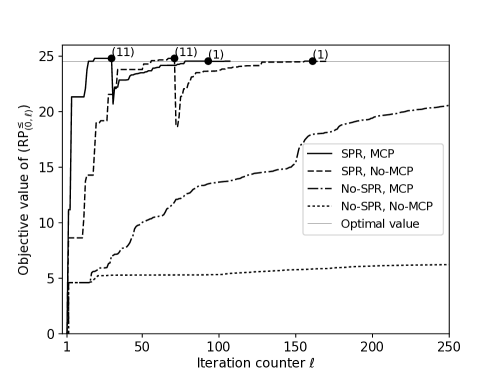
Figure 2. Column generation for Les Misérables instance (ID 13).

This figure clearly indicates the positive effect of the set-packing relaxation. For this case, our algorithm with the set-packing relaxation and without the multiple-cutting-planes-at-a-time has required the least computation time in spite of more iterations than that with the both techniques. That is since $($MILP subproblem and multiple cutting planes as columns$)$ is solved only once for each $\ell$, whereas the multiple-cutting-planes-at-a-time technique has to show that no column to be added is left for some $q^{\prime}$ after removing the vertices found at $q=1\ldots,q^{\prime}-1$ unless no column is found at $q=1$. We have observed a similar result for instance ID 15. For instance ID 13, the set-partitioning constraint set $V^{=}_{(b,\ell)}$ has been updated twice as it is depicted in the figure. We note that $V^{=}_{(b,\ell)}$ has been updated at most once for all the other solved instances.

4.4. Column generation as heuristics

For the unsolved instance IDs 17 and 18 applied to our branch-and-price framework, $($Set-packing relaxation of restricted master$)$ is solved instantly after the timeout. Table 5 shows lower bounds of the objective value obtained in this way. The best result for each instance is marked in bold.

Table 5. Lower bound values calculated after timeout of 3,600 seconds.

ID	CG-$($MILP subproblem and multiple cutting planes as columns$)$
	SPR	SPR	No-SPR	No-SPR
	MCP	No-MCP	MCP	No-MCP
17	$-33.63636$	$-33.63636$	6.63063	6.63063
18	27.05238	13.50693	3.57018	3.57018

These values have not exceeded those obtained by Santiago and Lamb (2017). This fact shows that the column generation is not necessarily a better heuristic method than the state-of-the-art heuristics for instances that cannot be exactly optimized.

5. Concluding Remarks

This paper has presented an exact algorithm for the modularity density maximization to provide a clustering solution of an undirected graph. The problem can be modeled as the ILP formulation of the set-partitioning problem, and we have proposed a branch-and-price framework for that. The acceleration techniques called the set-packing relaxation and the multiple-cutting-planes-at-a-time, combined with the newly introduced simpler MILP formulation of the column generation subproblem which is solved repeatedly, have enabled us to find the new and optimal solutions for the famous test instances: Graph, Les Misérables, A00 main and Protein p53. Political books as well as Protein p53 instances that have over 100 vertices have been optimized in around four minutes by a PC. Our solution method is deterministic and the computation time is not affected by any stochastic behavior. For Protein p53 instance, column generation at the root node of the branch-and-bound tree has provided a fractional upper bound solution and our algorithm have found an integral optimal solution after branching, which justifies the branch-and-price.

Future work would include a combination of heuristics and our formulations with the acceleration techniques to find a column in the column generation phase for unsolved instances that have over 110 vertices. Such heuristic methods may avoid much computation time that is necessary if we try to find a column by solving our MILP or possibly any other optimization-based problems, for a given particular dual solution value of the restricted master problem. Nonetheless we must optimize the column generation subproblem expressed by any form at some iteration when we decide whether we can terminate the column generation or not. It is unclear if the optimization problem at that iteration is easy to solve.

References

- (1)
- Aloise et al. (2010) Aloise, D., Cafieri, S., Caporossi, G., Hansen, P., Perron, S. and Liberti, L. (2010). Column generation algorithms for exact modularity maximization in networks. Physical Review E, vol. 82, no. 4, 046112. doi:10.1103/PhysRevE.82.046112.
- Barnhart et al. (1998) Barnhart, C., Johnson, E. L., Nemhauser, G. L., Savelsbergh, M. W. P. and Vance, P. H. (1998). Branch-and-price: Column generation for solving huge integer programs. Operations Research, vol. 46, no. 3, pp. 316–329. doi:10.1287/opre.46.3.316.
- Billionnet and Elloumi (2007) Billionnet, A. and Elloumi, S. (2007). Using a mixed integer quadratic programming solver for the unconstrained quadratic 0-1 problem. Mathematical Programming, Series A, vol. 109, no. 1, pp. 55–68. doi:10.1007/s10107-005-0637-9.
- Costa (2014) Costa, A. (2014). Some remarks on modularity density. arXiv:1409.4063 [cs.SI].
- Costa (2015) Costa, A. (2015). MILP formulations for the modularity density maximization problem. European Journal of Operational Research, vol. 245, no. 1, pp. 14–21. doi:10.1016/j.ejor.2015.03.012.
- Costa et al. (2016) Costa, A., Kushnarev, S., Liberti, L. and Sun, Z. (2016). Divisive heuristic for modularity density maximization. Computers & Operations Research, vol. 71, pp. 100–109. doi:10.1016/j.cor.2016.01.009.
- Costa et al. (in press) Costa, A., Ng, T. S. and Foo, L. X. (in press). Complete mixed integer linear programming formulations for modularity density based clustering. Discrete Optimization. doi:10.1016/j.disopt.2017.03.002 (corrected proof, available online on April 24, 2017).
- Desrosiers and Lübbecke (2005) Desrosiers, J. and Lübbecke, M. E. (2005). A primer in column generation. In Desaulniers, G., Desrosiers, J. and Solomon, M. M. eds., Column Generation, Springer, New York, the U.S., chap. 1, pp. 1–32. doi:10.1007/0-387-25486-2_1.
- Dinkelbach (1967) Dinkelbach, W. (1967). On nonlinear fractional programming. Management Science, vol. 13, no. 7, pp. 492–498. doi:10.1287/mnsc.13.7.492.
- Fortunato and Barthélemy (2007) Fortunato, S. and Barthélemy, M. (2007). Resolution limit in community detection. Proceedings of the National Academy of Sciences, vol. 104, no. 1, pp. 36–41. doi:10.1073/pnas.0605965104.
- Gong et al. (2012) Gong, M., Cai, Q., Li, Y. and Ma, J. (2012). An improved memetic algorithm for community detection in complex networks. In Proceedings of 2012 IEEE Congress on Evolutionary Computation (CEC), Brisbane, Australia. doi:10.1109/CEC.2012.6252971.
- Good et al. (2010) Good, B. H., de Montjoye, Y.-A. and Clauset, A. (2010). Performance of modularity maximization in practical contexts. Physical Review E, vol. 81, no. 4, 046106. doi:10.1103/PhysRevE.81.046106.
- Gurobi Optimization (2017) Gurobi Optimization (2017). Gurobi Optimizer. Retrieved May 11, 2017, from http://www.gurobi.com/products/gurobi-optimizer.
- Izunaga et al. (2016) Izunaga, Y., Matsui, T. and Yamamoto, Y. (2016). A doubly nonnegative relaxation for modularity density maximization. Technical Report, Optimization Online. Retrieved May 11, 2017, from http://www.optimization-online.org/DB_HTML/2016/03/5368.html.
- Izunaga and Yamamoto (2017) Izunaga, Y. and Yamamoto, Y. (2017). A cutting plane algorithm for modularity maximization problem. Journal of the Operations Research Society of Japan, vol. 60, no. 1, pp. 24–42. doi:10.15807/jorsj.60.24.
- Karimi-Majd et al. (2015) Karimi-Majd, A.-M., Fathian, M. and Amiri, B. (2015). A hybrid artificial immune network for detecting communities in complex networks. Computing, vol. 97, no. 5, pp. 483–507. doi:10.1007/s00607-014-0433-6.
- Li et al. (2008) Li, Z., Zhang, S., Wang, R.-S., Zhang, X.-S. and Chen, L. (2008). Quantitative function for community detection. Physical Review E, vol. 77, no. 3, 036109. doi:10.1103/PhysRevE.77.036109.
- Li et al. (2015) Li, Z., Zhang, S., Wang, R.-S., Zhang, X.-S. and Chen, L. (2015). Erratum: Quantitative function for community detection [Phys. Rev. E 77, 036109 (2008)]. Physical Review E, vol. 91, no. 1, 019901. doi:10.1103/PhysRevE.91.019901.
- Liu and Zeng (2010) Liu, J. and Zeng, J. (2010). Community detection based on modularity density and genetic algorithm. In Proceedings of 2010 International Conference on Computational Aspects of Social Networks (CASoN), Taiyuan, China, pp. 29–32. doi:10.1109/CASoN.2010.14.
- Lübbecke and Desrosiers (2005) Lübbecke, M. E. and Desrosiers, J. (2005). Selected topics in column generation. Operations Research, vol. 53, no. 6, pp. 1007–1023. doi:10.1287/opre.1050.0234.
- du Merle et al. (1999) du Merle, O., Villeneuve, D., Desrosiers, J. and Hansen, P. (1999). Stabilized column generation. Discrete Mathematics, vol. 194, no. 1–3, pp. 229–237. doi:10.1016/S0012-365X(98)00213-1.
- Nemhauser and Wolsey (1999) Nemhauser, G. L. and Wolsey, L. A. (1999). Integer and Combinatorial Optimization. John Wiley & Sons, New York, the U.S.
- Newman and Girvan (2004) Newman, M. E. J. and Girvan, M. (2004). Finding and evaluating community structure in networks. Physical Review E, vol. 69, no. 2, 026113. doi:10.1103/PhysRevE.69.026113.
- Ryan and Foster (1981) Ryan, D. M. and Foster, B. A. (1981). An integer programming approach to scheduling. In Wren, A. ed., Computer Scheduling of Public Transport: Urban Passenger Vehicle and Crew Scheduling, North-Holland, Amsterdam, the Netherlands, pp. 269–280.
- Santiago and Lamb (2017) Santiago, R. and Lamb, L. C. (2017). Efficient modularity density heuristics for large graphs. European Journal of Operational Research, vol. 258, no. 3, pp. 844–865. doi:10.1016/j.ejor.2016.10.033.
- de Santiago and Lamb (in press) de Santiago, R. and Lamb, L. C. (in press). Exact computational solution of modularity density maximization by effective column generation. Computers & Operations Research. doi:10.1016/j.cor.2017.04.013 (accepted manuscript, available online on April 27, 2017).
- Sato and Fukumura (2012) Sato, K. and Fukumura, N. (2012). Real-time freight locomotive rescheduling and uncovered train detection during disruption. European Journal of Operational Research, vol. 221, no. 3, pp. 636–648. doi:10.1016/j.ejor.2012.04.025.
- Vanderbeck (2005) Vanderbeck, F. (2005). Implementing mixed integer column generation. In Desaulniers, G., Desrosiers, J. and Solomon, M. M. eds., Column Generation, Springer, New York, the U.S., chap. 12, pp. 331–358. doi:10.1007/0-387-25486-2_12.