Analysis of the strong vertexes of $\Sigma_{c}^{*}ND$ and $\Sigma_{b}^{*}NB$ in QCD sum rules

Abstract

In this article, we analyze the strong vertexes $\Sigma_{c}^{*}ND$ and $\Sigma_{b}^{*}NB$ using the three-point QCD sum rules under the Dirac structure of $q\!\!\!/p\!\!\!/\gamma_{\mu}$. We perform our analysis by considering the contributions of the perturbative part and the condensate terms of $<\overline{q}q>$ and $<\frac{\alpha_{s}}{\pi}GG>$. After the form factors are calculated, they are then fitted into analytical functions which are used to get the strong coupling constants for these two vertexes. The final results are $g_{\Sigma_{c}^{*}ND}=7.19^{+8.49}_{-3.11}\pm 1.76$ and $g_{\Sigma_{b}^{*}NB}=10.54^{+15.59}_{-5.23}\pm 1.82$.

1 Introduction

The charmed and bottom baryons, which contain at least a heavy quark, serve as a particular laboratory for studying dynamics of the light quarks in the presence of the heavy quark(s), and also as an excellent ground for testing predictions of the quark model and heavy quark symmetry. The properties of these heavy baryon states mainly include the mass spectrum, the magnetic moments, the strong, electromagnetic and weak decay behaviors. Investigation of these properties can give us useful information on the quark structure of these baryons. The strong coupling constants is an important parameter about the strong interactions of the heavy baryons. The accurate determination of the coupling constants can not only help us further understanding the strong decay behaviors of these heavy baryons but also give us the knowledge about its nature and structure.

By this time, many heavy baryon states have been discovered in experiments by BaBar, Belle, CDF and D0 CollaborationsAube06 ; Naka10 ; Lesi ; Rosn07 . These states include the charmed baryons such as $\frac{1}{2}^{+}$ antitriplet states($\Lambda^{+}_{c}$,$\Xi^{+}_{c}$,$\Xi^{0}_{c}$), the $\frac{1}{2}^{+}$ and $\frac{3}{2}^{+}$ sextet states ($\Omega_{c}$,$\Sigma_{c}$,$\Sigma^{\prime}_{c}$) and ($\Omega^{*}_{c}$,$\Sigma^{*}_{c}$,$\Sigma^{*}_{c}$)Naka10 . Besides, CDF and LHCb Collaborations observed several S-wave bottom baryon states, $\Lambda_{b}$,$\Sigma_{b}$,$\Sigma^{*}_{b}$,$\Xi_{b}$ and $\Omega_{b}$Paul ; Klem10 . The SELEX collaboration even reported the observation of the signal for the doubly charmed baryon state $\Xi_{cc}^{+}$Matt ; Oche . Stimulated by these discoveries, theorists studied the nature of these baryons with different theoretical approachesFaes ; Pate ; LiuX ; ChenHX1 ; Chun ; ChenW ; Zhjr ; Karl1 ; Karl2 ; Nava ; Khod ; Alie ; Azi1 ; Azi2 ; Wzg ; KangXW ; Esposito . As mentioned above, the subsequent analysis of the strong decays of these baryons requires knowledge about their strong coupling constants. Thus, people calculated some of the strong coupling constants, $g_{\Omega^{*}_{c}\Omega^{*}_{c}\phi}$,$g_{\Omega^{*}_{c}\Xi^{*}_{c}K^{*}}$, $g_{\Xi^{*}_{c}\Sigma^{*}_{c}K^{*}}$,$g_{\Omega^{*}_{b}\Omega^{*}_{b}\phi}$,$g_{\Xi^{*}_{b}\Sigma^{*}_{b}K^{*}}$,$g_{\Xi^{*}_{b}\Xi_{b}\pi}$,$g_{\Xi^{*}_{c}\Xi_{c}\pi}$, $g_{\Lambda_{b}NB^{*}}$,$g_{\Lambda_{b}N^{*}B^{*}}$,$g_{\Lambda_{c}ND^{*}}$,$g_{\Lambda_{c}N^{*}D^{*}}$,$g_{\Sigma_{c}ND^{*}}$,$g_{\Sigma_{b}N^{*}B^{*}}$, $g_{\Sigma_{b}NB^{*}}$ and $g_{\Sigma_{c}N^{*}D^{*}}$, etcAzi1 ; Azi2 ; Wzg5 ; Navar ; Khodj ; GuoLY2 ; Azizi4 . For these work, QCD sum rules proved to be a most powerful nonperturbative method which has been widely used to analyze the properties of the hadronsBrac1 ; Brac2 ; Alie2 ; Alie3 ; Alie4 ; Doi ; Altm ; Wzg3 ; Cerq ; Rodr ; Yazi ; Khos1 ; Khos2 ; Rein ; Pasc ; Wzg4 ; Guoly .

In the present paper, we calculate the strong coupling constants $g_{\Sigma_{c}^{*}ND}$ and $g_{\Sigma_{b}^{*}NB}$ within the framework of the QCD sum rules. The results of this work are relevant in the bottom and charmed meson cloud description of the nucleon which may be used to explain exotic events observed by different collaborations. Besides, the exact values of these strong coupling constants are essential to determine the modifications on the masses, decay constants and other parameters of the $B$ and $D$ mesons in nuclear mediumWzgH ; Kuma ; Haya . The layout of this paper is as follows. The next section presents the details of the analysis of the vertexes $\Sigma_{c}^{*}ND$ and $\Sigma_{b}^{*}NB$. In Sec.3, we present the numerical results and discussions, and Sec.4 is reserved for our conclusions.

2 QCD sum rules for $\Sigma_{c}^{*}ND$ and $\Sigma_{b}^{*}NB$

We study the strong coupling constants of the vertexes $\Sigma_{c}^{*}ND$ and $\Sigma_{b}^{*}NB$ with the following three-point correlation function,

$$\Pi_{\mu}(p,p^{\prime},q)=i^{2}\int d^{4}x\int d^{4}ye^{-ip.x}e^{ip^{\prime}.y}\Big{\langle}0|\mathcal{T}\Big{(}J_{N}(y)J_{D[B]}(0)\overline{J}_{\mu\Sigma_{c}^{*}[\Sigma_{b}^{*}]}(x)\Big{)}|0\Big{\rangle},$$ (1)

where $\mathcal{T}$ is the time ordered product and $J_{\mu\Sigma_{c}^{*}[\Sigma_{b}^{*}]}$, $J_{N}$ and $J_{D[B]}$ are the interpolating currents of the baryons $\Sigma_{c}^{*}[\Sigma_{b}^{*}]$, $N$ and the meson $D[B]$. Baryon current is a composite operator with the same quantum numbers as a given baryon, which include several possibilitiesIoff1 ; Cola . For simplicity, the interpolating currents used in Equation(1) are written as the following form,

$$J_{\mu\Sigma_{c}^{*}[\sum_{b}^{*}]}(x)=\epsilon_{ijk}\Big{(}u^{iT}(x)C\gamma_{\mu}d^{j}(x)\Big{)}c[b]^{k}(x),$$

$$J_{N}(y)=\epsilon_{ijk}\Big{(}u^{iT}(y)C\gamma_{\mu}u^{j}(y)\Big{)}\gamma_{5}\gamma^{\mu}d^{k}(y),$$

$$J_{D[B]}(0)=\overline{u}(0)\gamma_{5}c[b](0).$$ (2)

The correlation function will be calculated in two different ways, from the hadron degrees of freedom and quark degrees of freedom, which are called the phenomenological side and the operator product expansion(OPE) side separately.

2.1 The phenomenological side

In order to obtain the phenomenological representations, we insert a complete set of intermediate hadronic states with the same quantum numbers as the current operators $J_{\mu\Sigma_{c}^{*}[\Sigma_{b}^{*}]}$, $J_{N}$ and $J_{D[B]}$ into the correlation $\Pi_{\mu}(p,p^{\prime},q)$. Then, after the ground-state contributions are isolated, we get the following function.

$$\Pi^{HAD}_{\mu}(p,p^{\prime},q)= \frac{\Big{\langle}0|J_{N}|N(p^{\prime})\Big{\rangle}\Big{\langle}0|J_{D[B]}|D[B](q)\Big{\rangle}\Big{\langle}\Sigma_{c}^{*}[\Sigma_{b}^{*}](p)|\overline{J}_{\mu\Sigma_{c}^{*}[\Sigma_{b}^{*}]}|0\Big{\rangle}}{(p^{2}-m^{2}_{\Sigma_{c}^{*}[\Sigma_{b}^{*}]})(p^{\prime 2}-m^{2}_{N})(q^{2}-m^{2}_{D[B]})}$$ (3)

$$\Big{\langle}N(p^{\prime})D[B](q)|\Sigma_{c}^{*}[\Sigma_{b}^{*}](p)\Big{\rangle}+\cdots$$

Where $h.r.$ stands for the contributions of the higher resonances and continuum states. After the matrix elements appearing in the above equation are substituted for the following parameterized equations,

$$\langle 0|J_{N}|N(p^{\prime})\rangle=\lambda_{N}u_{N}(p^{\prime},s^{\prime}),$$

$$\langle 0|J_{D[B]}|D[B](q)\rangle=i\frac{m_{D[B]}^{2}f_{D[B]}}{m_{u}+m_{c[b]}},$$

$$\langle\Sigma_{c}^{*}[\Sigma_{b}^{*}](p)|\overline{J}_{\mu\Sigma_{c}^{*}[\Sigma_{b}^{*}]}|0\rangle=\lambda_{\Sigma_{c}^{*}[\Sigma_{b}^{*}]}\overline{u}_{\mu\Sigma_{c}^{*}[\Sigma_{b}^{*}]}(p,s),$$

$$\langle N(p^{\prime})D[B](q)|\Sigma_{c}^{*}[\Sigma_{b}^{*}](p)\rangle=ig_{\Sigma_{c}^{*}ND[\Sigma_{b}^{*}NB]}\overline{u}_{N}(p^{\prime},s^{\prime})u_{\Sigma_{c}^{*}[\Sigma_{b}^{*}]\alpha}(p,s)q^{\alpha},$$ (4)

the correlation function $\Pi_{\mu}(p,p^{\prime},q)$ can be decomposed as

$$\Pi^{HAD}_{\mu}(p,p^{\prime},q)= i^{2}\frac{Cg_{\Sigma_{c}^{*}ND[\Sigma_{b}^{*}NB]}}{(p^{2}-m^{2}_{\Sigma_{c}^{*}[\Sigma_{b}^{*}]})(p^{\prime 2}-m^{2}_{N})(q^{2}-m^{2}_{D[B]})}$$ (5)

$$\times\Big{\{}\Pi_{1}q_{\mu}+\Pi_{2}p\!\!\!/q_{\mu}+\Pi_{3}q\!\!\!/q_{\mu}+\Pi_{4}q\!\!\!/p\!\!\!/q_{\mu}$$

$$+\Pi_{5}p_{\mu}+\Pi_{6}p\!\!\!/p_{\mu}+\Pi_{7}q\!\!\!/p_{\mu}+\Pi_{8}q\!\!\!/p\!\!\!/p_{\mu}$$

$$+\Pi_{9}\gamma_{\mu}+\Pi_{10}p\!\!\!/\gamma_{\mu}+\Pi_{11}q\!\!\!/\gamma_{\mu}+\Pi_{12}q\!\!\!/p\!\!\!/\gamma_{\mu}\Big{\}}$$

$$+\cdots.$$

Where $C=\frac{m_{D[B]}^{2}f_{D[B]}\lambda_{N}\lambda_{\Sigma_{c}^{*}[\Sigma_{b}^{*}]}}{m_{c[b]}+m_{u}}$, and some of the Dirac structure appearing in the above function are written as

$$\Pi_{1}=(m_{\Sigma_{c}^{*}[\Sigma_{b}^{*}]}+m_{N})m_{\Sigma_{c}^{*}[\Sigma_{b}^{*}]},$$

$$\Pi_{2}=(m_{\Sigma_{c}^{*}[\Sigma_{b}^{*}]}+m_{N}),$$

$$\Pi_{i}=\cdots\cdots\cdots\cdots,$$

$$\Pi_{12}=\frac{m_{\Sigma_{c}^{*}[\Sigma_{b}^{*}]}^{2}+2m_{\Sigma_{c}^{*}[\Sigma_{b}^{*}]}m_{N}+m_{N}^{2}-q^{2}}{6m_{\Sigma_{c}^{*}[\Sigma_{b}^{*}]}}.$$ (6)

In our previous analysis about this kind of problem, we found that the Dirac structure $q\!\!\!/p\!\!\!/\gamma_{\mu}$ can not lead to contaminations for $\Sigma_{c}^{*}[\Sigma_{b}^{*}]$WangZG5 . Thus, we choose the Dirac structure $q\!\!\!/p\!\!\!/\gamma_{\mu}$ to carry out our analysis. In this above derivation, we also use the following definitions,

$$\Sigma u_{N}(p^{\prime},s^{\prime})\overline{u}_{N}(p^{\prime},s^{\prime})=p\!\!\!/^{\prime}+m_{N},$$

$$\Sigma u_{\alpha\Sigma_{c}^{*}[\Sigma_{b}^{*}]}(p,s)\overline{u}_{\mu\Sigma_{c}^{*}[\Sigma_{b}^{*}]}(p,s)=-(p\!\!\!/+m_{\Sigma_{c}^{*}[\Sigma_{b}^{*}]})(g_{\alpha\mu}-\frac{\gamma_{\alpha}\gamma_{\mu}}{3m_{\Sigma_{c}^{*}[\Sigma_{b}^{*}]}}-\frac{2p_{\alpha}p_{\mu}}{3m^{2}_{\Sigma_{c}^{*}[\Sigma_{b}^{*}]}}+\frac{p_{\alpha}\gamma_{\mu}-\gamma_{\alpha}p_{\mu}}{3m_{\Sigma_{c}^{*}[\Sigma_{b}^{*}]}})$$ (7)

2.2 The OPE side

We carry out the operator product expansion of the correlation function in deep Euclidean region, where $p^{2}\rightarrow-\infty$ and $p^{\prime 2}\rightarrow-\infty$. Considering all possible contractions of the quark fields with Wick’s theorem, the correlation function Eq.$(1)$ is written as

$$\ \Pi_{\mu}^{OPE}(p,p^{\prime},q)= i^{2}\int d^{4}x\int d^{4}ye^{-ip.x}e^{ip^{\prime}.y}\epsilon_{abc}\epsilon_{ijk}$$ (8)

$$\times\Big{\{}\gamma_{5}\gamma_{\nu}S_{d}^{cj}(y-x)\gamma_{\mu}CS_{u}^{biT}(y-x)C\gamma_{\nu}S_{u}^{ah}(y)\gamma_{5}S_{c[b]}^{hk}(-x)$$

$$-\gamma_{5}\gamma_{\nu}S_{d}^{cj}(y-x)\gamma_{\mu}CS_{u}^{aiT}(y-x)C\gamma_{\nu}S_{u}^{bh}(y)\gamma_{5}S_{c[b]}^{hk}(-x)\Big{\}}$$

Then, we replace the $c[b]$ and $u[d]$ quark propagators with the corresponding full propagatorsPasc ; Wzg4 ; Rein ,

$$S_{c[b]}^{mn}(x)= \frac{i}{(2\pi)^{4}}\int d^{4}ke^{-ik.x}\Big{\{}\frac{\delta_{mn}}{k\!\!\!/-m_{b[c]}}-\frac{g_{s}G_{mn}^{\alpha\beta}}{4}\frac{\sigma_{\alpha\beta}(k\!\!\!/+m_{b[c]})+(k\!\!\!/+m_{b[c]})\sigma_{\alpha\beta}}{(k^{2}-m_{Q}^{2})^{2}}$$ (9)

$$+\frac{\pi^{2}}{3}\Big{\langle}\frac{\alpha_{s}GG}{\pi}\Big{\rangle}\delta_{mn}m_{b[c]}\frac{k^{2}+m_{b[c]}k\!\!\!/}{(k^{2}-m_{b[c]}^{2})^{4}}+\cdots\Big{\}},$$

$$S_{u[d]}^{mn}(x)= i\frac{x\!\!\!/}{2\pi^{2}x^{4}}\delta_{mn}-\frac{m_{u[d]}}{4\pi^{2}x^{2}}\delta_{mn}-\frac{\langle\overline{q}q\rangle}{12}\Big{(}1-i\frac{m_{u[d]}}{4}x\!\!\!/\Big{)}-\frac{x^{2}}{192}m_{0}^{2}\langle\overline{q}q\rangle\Big{(}1-i\frac{m_{u[d]}}{6}x\!\!\!/\Big{)}$$

$$-\frac{ig_{s}\lambda_{A}^{ij}G^{A}_{\theta\eta}}{32\pi^{2}x^{2}}\Big{[}x\!\!\!/\sigma^{\theta\eta}+\sigma^{\theta\eta}x\!\!\!/\Big{]}+\cdots.$$

In order to perform the four-$x$ and four-$y$ integrals, we also use the following Fourier transformations in $D=4+\epsilon$ dimensions with $\epsilon\rightarrow 0$,

$$\frac{1}{[(y-x)^{2}]^{n}}=\int\frac{d^{D}t}{(2\pi)^{D}}e^{-it.(y-x)}i(-1)^{n+1}2^{D-2n}\pi^{D/2}\frac{\Gamma(D/2-n)}{\Gamma(n)}\Big{(}-\frac{1}{t^{2}}\Big{)}^{D/2-n},$$ (11)

$$\frac{1}{[y^{2}]^{n}}=\int\frac{d^{D}t^{\prime}}{(2\pi)^{D}}e^{-it^{\prime}.y}i(-1)^{n+1}2^{D-2n}\pi^{D/2}\frac{\Gamma(D/2-n)}{\Gamma(n)}\Big{(}-\frac{1}{t^{\prime 2}}\Big{)}^{D/2-n},$$ (12)

which is followed by the replacements $x_{\mu}\rightarrow i\frac{\partial}{\partial p_{\mu}}$ and $y_{\mu}\rightarrow-i\frac{\partial}{\partial p^{\prime}_{\mu}}$. After these derivations, these integrals turn into Dirac delta functions which are used to take the four-integrals over $k$ and $t^{\prime}$. Finally, the Feynman parametrization and

$$\ \int\frac{d^{D}t}{(2\pi)^{D}}\frac{1}{[t-M^{2}]^{\alpha}} =\frac{i(-1)^{\alpha}}{(4\pi)^{D/2}}\frac{\Gamma(\alpha-D/2)}{\Gamma(\alpha)}\frac{1}{(M^{2})^{\alpha-D/2}}$$

is used to perform the four-$t$ integral. After a lengthy derivation, we obtain the same Dirac structures as the phenomenological side(see Eq.$(5)$). For each Dirac structure, the correlation function can be divided into two parts,

$$\Pi^{OPE}_{i}=\Pi^{pert}_{i}+\Pi^{non-pert}_{i}$$ (13)

Where $i$ stands for different Dirac structure in Eq.$(5)$. Using dispersion relations, the perturbative term for a given Dirac structure can be written as the following form,

$$\Pi^{pert}_{i}(q^{2})=\int_{s_{1}}^{s_{0}}ds\int_{u_{1}}^{u_{0}}du\frac{\rho_{i}^{pert}(s,u,q^{2})}{(s-p^{2})(u-p^{\prime 2})}$$ (14)

where $\rho_{i}^{pert}(s,u,q^{2})$, appearing in the above equation, is the spectral density which is obtained from the imaginary part of the correlation. After these derivations, we set $s=p^{2}$, $u=p^{\prime 2}$ and $q=p-p^{\prime}$ in the spectral densities. For the Dirac structure of $q\!\!\!/p\!\!\!/\gamma_{\mu}$, its spectral density is written as,

$$\ \rho_{q\!\!\!/p\!\!\!/\gamma_{\mu}}^{pert}(s,u,q^{2}) =\frac{3}{32\pi^{4}}\int^{1}_{0}dx\int^{1-x}_{0}\Big{\{}\frac{x+y}{2(x+y-1)}\Big{[}x(-q^{2}y+m_{c[b]^{2}})-sx(x+y-1)-uy(x+y-1)\Big{]}$$

$$+\frac{1}{6}\Big{[}sx(x+y)+uy(x+y)+q^{2}xy-6m_{d}m_{u}\Big{]}\Big{\}}dy\times\Theta[H_{2}(s,u,q^{2})],$$ (15)

where $\Theta$ stands for the unit-step function, and $H_{2}(s,u,q^{2})$ is defined as $H_{2}[s,u,q^{2}]=x(m_{c[b]}^{2}-q^{2}y)+sx(x+y-1)+uy(x+y-1)$. Considering the limit of the unit-function to the integrals, the integral limmits for parameter $y$ can be explicitly expressed as

$$0\leq y\leq min\Big{\{}1-x,\frac{[(s+u-q^{2})-u]-\sqrt{\Delta}}{-2u}\Big{\}}$$ (16)

where $\Delta=\Big{[}(s+u-q^{2})^{2}-4su\Big{]}x^{2}-2u\Big{[}(s+u-q^{2})+2m_{c[b]}^{2}\Big{]}x+4su+u^{2}$.

From our previous analysis, the non-perturbative contributions comes mainly from the $<\overline{q}q>$. Besides of this condensate term, we also take into account the contribution from $<\frac{\alpha_{s}}{\pi}GG>$ in this work. For these condensate terms, we make the change of variables $p^{2}\rightarrow-P^{2}$, $p^{\prime 2}\rightarrow-P^{\prime 2}$ and $q^{2}\rightarrow-Q^{2}$ and perform a double Borel transform to them, which involves the transformation: $P^{2}\rightarrow M_{1}^{2}$ and $P^{\prime 2}\rightarrow M_{2}^{2}$, where $M_{1}$ and $M_{2}$ are the Borel parameters. Then, the non-perturbative terms can be written as,

$$\ \mathscr{B}\mathscr{B}\Big{[}\Pi_{q\!\!\!/p\!\!\!/\gamma_{\mu}}^{<\overline{q}q>}(Q^{2})\Big{]} =\frac{<\overline{q}q>}{64\pi^{2}}\int^{1}_{0}dx\int^{1-x}_{0}\Big{\{}\frac{4\Big{[}(12m_{d}+3m_{u})(x+y-1)+14m_{d}+5m_{u}\Big{]}}{x+y}$$

$$+(4m_{u}+16m_{d})\Big{[}1+\frac{x(Q^{2}y+m_{c[b]}^{2})}{x(x+y-1)M_{1}^{2}}-\frac{y}{x+y}\frac{Q^{2}}{M_{1}^{2}}\Big{]}\Big{\}}dy$$

$$\times\frac{e^{\frac{Q^{2}y+m_{c[b]}^{2}}{(x+y-1)M_{1}^{2}}}}{M_{1}^{2}+M_{2}^{2}}\delta\Big{\{}k-\frac{M_{2}^{2}}{M_{1}^{2}+M_{2}^{2}}\Big{\}},$$

$$\ \mathscr{B}\mathscr{B}\Big{[}\Pi_{q\!\!\!/p\!\!\!/\gamma_{\mu}}^{<\overline{G}G>}(Q^{2})\Big{]} =\frac{<\frac{\alpha_{s}}{\pi}GG>}{32\pi^{2}\times 48}\int^{1}_{0}dx\int^{1-x}_{0}\Big{\{}\frac{x^{2}}{6(x+y-1)^{3}}\Big{[}8+\frac{2x(Q^{2}y+m_{c[b]}^{2})}{x(x+y-1)M_{1}^{2}}-\frac{y}{x+y}\frac{Q^{2}}{M_{1}^{2}}\Big{]}$$

$$\times\frac{m_{c[b]}^{2}}{M_{1}^{2}}\Big{\}}dy\frac{e^{\frac{Q^{2}y+m_{c[b]}^{2}}{(x+y-1)M_{1}^{2}}}}{M_{1}^{2}+M_{2}^{2}}\delta\Big{\{}k-\frac{M_{2}^{2}}{M_{1}^{2}+M_{2}^{2}}\Big{\}},$$

where $\mathscr{B}\mathscr{B}[$ $]$ stands for the double Borel transform, $\delta$ is the Delta function and $k=\frac{x}{x+y}$.

2.3 The strong coupling constant

3 The results and discussions

We perform a double Borel transform to the phenomenological side as well as the OPE side, after which we equate these two sides, invoking the quark-hadron duality. After these preformation, the form factor can be written as,

$$g_{\Sigma_{c}^{*}ND(\Sigma_{b}^{*}NB)}(Q^{2})$$

$$=\frac{\frac{1}{M_{1}^{2}M^{2}_{2}}\int_{(m_{c[b]}+m_{u}+m_{d})^{2}}^{s_{0}}\int_{(2m_{u}+m_{d})^{2}}^{u_{0}}\rho_{i}^{pert}(s,u,Q^{2})e^{-\frac{s}{M_{1}^{2}}}e^{-\frac{u}{M_{2}^{2}}}dsdu+\mathscr{B}\mathscr{B}\Big{[}\Pi^{non-pert}(Q^{2})\Big{]}}{\frac{C\Pi_{12}}{(Q^{2}+m_{D[B]}^{2})M_{1}^{2}M_{2}^{2}}e^{-\frac{m_{\Sigma_{c}^{*}[\Sigma_{b}^{*}]}^{2}}{M_{1}^{2}}}e^{-\frac{m_{N}^{2}}{M_{2}^{2}}}}$$ (19)

Where $\Pi_{12}$ in the above equation represents the $q\!\!\!/p\!\!\!/\gamma_{\mu}$ term in the phenomenological side in Eq.$(5)$, $s_{0}$ and $u_{0}$ are the continuum threshold parameters which are used to eliminate the $h.r.$ terms. Commonly, the continuum parameters, $s_{0}=(m_{i}+\Delta_{i})^{2}$ and $u_{0}=(m_{o}+\Delta_{o})^{2}$ are employed to include the pole and suppress the $h.r.$ contributions, where $m_{i}$ and $m_{o}$ are the masses of the incoming and out-coming baryons respectively. In general, $\Delta_{i}$ and $\Delta_{o}$ are chosen to be about $0.5GeV^{2}$ for mesons, whose value is some what smaller than that of the baryons.

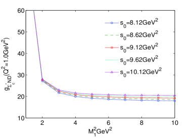
Figure 1: The strong form factor $g_{\Sigma_{c}^{*}ND}$ on Borel parameter $M_{1}^{2}$, in the different values of $s_{0}$.

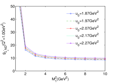
Figure 2: The strong form factor $g_{\Sigma_{c}^{*}ND}$ on Borel parameter $M_{1}^{2}$, in the different values of $u_{0}$.

It can also be seen from Eq.$(19)$ that the form factor $g_{\Sigma_{c}^{*}ND[\Sigma_{b}^{*}NB]}$ is the function of the Borel parameters $M_{1}^{2}$ and $M_{2}^{2}$. We determine the working regions for the Borel parameters according to two considerations which are pole dominance and convergence of the OPE. That is to say, the pole contribution should be as large as possible comparing with the contributions of the higher and continuum states. Meanwhile, we should also find a plateau, which will ensure OPE convergence and the stability of our results. The plateau is often called ”Borel window”.

The form factor, $g_{\Sigma_{c}^{*}ND}$, on Borel parameter $M_{1}^{2}$ in the different values of $s_{0}$ and $u_{0}$ are shown in Figs.1 and 2, where $9.12GeV^{2}\approx(m_{\Sigma_{c}^{*}}+0.5GeV)^{2}$ and $2.07GeV^{2}\approx(m_{D}+0.5GeV)^{2}$ in these figures. It can be seen from Fig.1 that the value of $g_{\Sigma_{c}^{*}ND}$ show more stability with $s_{0}=10.12GeV^{2}$. However, we can see from Fig.2 that the line of $g_{\Sigma_{c}^{*}ND}$ show little change with $u_{0}$ changes from $1.87GeV^{2}$ to $2.27GeV^{2}$. Finally, the continuum threshold parameters are chosen to be $u_{0}=2.07GeV^{2}$ and $s_{0}=10.12GeV^{2}[39.00GeV^{2}]$ for vertex $\Sigma_{c}^{*}ND[\Sigma_{b}^{*}NB]$. In Figs.$3-6$, we show also the relative continuum and pole contribution on Borel parameter. We can see from these figures that the more little values of the Borel parameters lead to larger pole contributions in the results. However, if too little values of the Borel parameters are taken(see Figs.1 and 2), the results decrease monotonously and quickly with the Borel parameters, which means that the convergence of the OPE can not be satisfied. Finally, the Borel windows are chosen to be $3.0GeV^{2}<M_{1}^{2}<5.0GeV^{2}$ and $1.0GeV^{2}<M_{2}^{2}<3.0GeV^{2}$ for the vertex $\Sigma_{c}^{*}ND$, and $9.0GeV^{2}<M_{1}^{2}<11.0GeV^{2}$ and $1.0GeV^{2}<M_{2}^{2}<3.0GeV^{2}$ for the vertex $\Sigma_{b}^{*}NB$. Under these circumstances the criteria of pole dominance and OPE convergence are all satisfied. It can also be seen from Figs.7-9 that our results have weak dependence on the Borel parameters, which indicates the stability of the results.

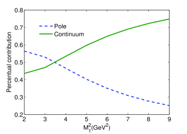
Figure 3: Pole and continuum contributions for vertex $\Sigma_{c}^{*}ND$, on Borel parameter $M_{1}^{2}$.

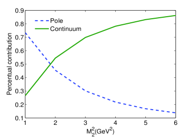
Figure 4: Pole and continuum contributions for vertex $\Sigma_{c}^{*}ND$, on Borel parameter $M_{2}^{2}$.

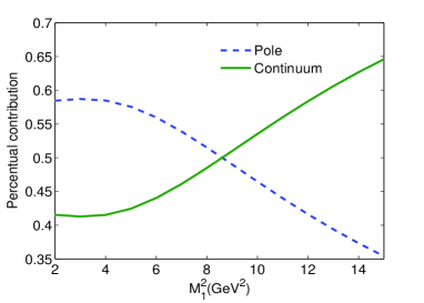
Figure 5: Pole and continuum contributions for vertex $\Sigma_{b}^{*}NB$, on Borel parameter $M_{1}^{2}$.

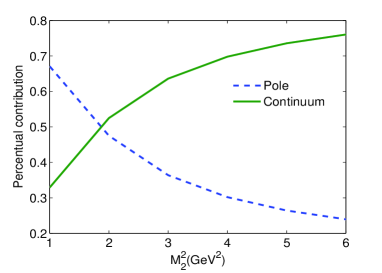
Figure 6: Pole and continuum contributions for vertex $\Sigma_{b}^{*}NB$, on Borel parameter $M_{2}^{2}$

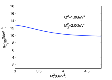
Figure 7: $g_{\Sigma_{c}^{*}ND}$ ($Q^{2}=1.0GeV^{2}$) as a function of the Borel mass $M_{1}^{2}$.

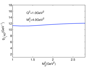
Figure 8: $g_{\Sigma_{c}^{*}ND}$ ($Q^{2}=1.0GeV^{2}$) as a function of the Borel mass $M_{2}^{2}$

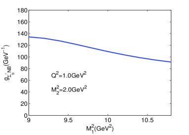
Figure 9: $g_{\Sigma_{b}^{*}NB}$ ($Q^{2}=1.0GeV^{2}$) as a function of the Borel mass $M_{1}^{2}$

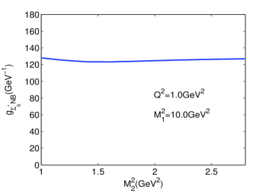
Figure 10: $g_{\Sigma_{b}^{*}NB}$ ($Q^{2}=1.0GeV^{2}$) as a function of the Borel mass $M_{2}^{2}$

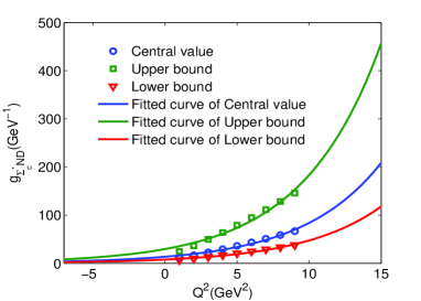
Figure 11: The form factor for the vertex $\Sigma_{c}^{*}ND$, and its fitted results as a function of $Q^{2}$.

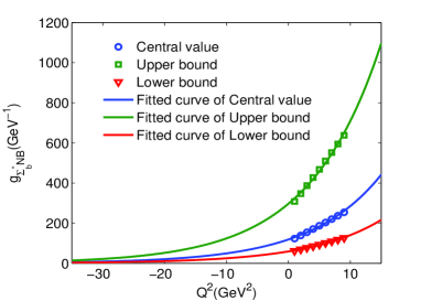
Figure 12: The form factor for the vertex $\Sigma_{b}^{*}NB$, and its fitted results as a function of $Q^{2}$.

Table 1: Input parameters used in this analysis.

Parameters	Values
$m_{\Sigma_{b}^{*}}$	$5835.1\pm 1.9$ $MeV$ Oliv
$m_{\Sigma_{c}^{*}}$	$2517.5\pm 2.3$ $MeV$ Oliv
$m_{N}$	$939.565379\pm 0.000021$ $MeV$ Oliv
$m_{D}$	$1864.86\pm 0.13$ $MeV$ Oliv
$m_{B}$	$5279.58\pm 0.17$ $MeV$ Oliv
$m_{b}$	$4.18\pm 0.03$ $GeV$ Oliv
$m_{c}$	$1.275\pm 0.025$ $GeV$ Oliv
$m_{d}$	$4.8^{+0.5}_{-0.3}$ $MeV$ Oliv
$m_{u}$	$2.3^{+0.7}_{-0.5}$ $MeV$ Oliv
$\langle\overline{u}u\rangle$	$-(0.24\pm 0.01)GeV^{3}$Ioff2
$\langle\overline{d}d\rangle$	$-(0.24\pm 0.01)GeV^{3}$ Ioff2
$\langle\frac{\alpha_{s}G^{2}}{\pi}\rangle$	$(0.012\pm 0.04)$ $GeV^{4}$ Bely
$\lambda_{\Sigma_{b}^{*}}$	$0.0125^{+0.0008}_{-0.0004}GeV^{3}$ WangZG
$\lambda_{\Sigma_{c}^{*}}$	$0.0246^{+0.0022}_{-0.0016}GeV^{3}$ WangZG
$\lambda_{N}^{2}$	$0.0011\pm 0.0005$ $GeV^{6}$ Azi3
$f_{B}$	($248\pm 23_{exp}\pm 25_{Vub}$) $MeV$ Khod4
$f_{D}$	($205.8\pm 8.5\pm 2.5$) $MeV$ Eise

In order to obtain the coupling constants, it is necessary to extrapolate these calculated results of the form factors into the deep time-like regions by fitting these results into analytical functions. The extrapolation to deep time-like regions is highly mode-dependent, thus there is no specific expressions for the dependence of the strong form factors on $Q^{2}$. From our analysis, we observe that this dependence can be well described by the following fit function

$$g_{\Sigma_{c}^{*}ND(\Sigma_{b}^{*}NB)}(Q^{2})=A_{c(b)}exp[{B_{c(b)}Q^{2}}]$$ (20)

The fitted results for $g_{\Sigma_{c}^{*}ND}$ and $g_{\Sigma_{b}^{*}NB}$ are $A_{c}=13.54\pm 3.00$$GeV^{-1}$, $B_{c}=0.1824\pm 0.03$$GeV^{-2}$, and $A_{b}=118.60\pm 5.00$$GeV^{-1}$, $B_{b}=0.08675\pm 0.006$$GeV^{-2}$. In Figs.11 and 12, we show the dependence of the strong coupling form factors on $Q^{2}$ for both the QCD sum rules and fitting results, in which it is marked as Central value and fitted curve of Central value. The values of the strong coupling constants can be obtained from the fit function at $Q^{2}=-m_{B[D]}^{2}$, which are $g_{\Sigma_{c}^{*}ND}=7.19\pm 1.76$ and $g_{\Sigma_{b}^{*}NB}=10.54\pm 1.82$. The errors appearing in these results are coming from the uncertainties of the fitting parameters of $\delta A_{c}$, $\delta B_{c}$, $\delta A_{b}$ and $\delta B_{b}$.

The uncertainties of the results coming from the input parameters can be estimated with the formula $\delta=\sqrt{\Sigma_{i}(\frac{\partial f}{\partial x_{i}})^{2}(x_{i}-\overline{x}_{i})^{2}}$, where the $f$ denotes strong form factors $g_{\Sigma_{c}^{*}ND}$ and $g_{\Sigma_{b}^{*}NB}$, the $x_{i}$ denotes the revelent parameters $m_{\Sigma_{b}^{*}}$,$m_{\Sigma_{c}^{*}}$,$m_{b}$,$m_{c}$,$\lambda_{\Sigma_{b}^{*}}$, $\lambda_{\Sigma_{c}^{*}}$,$\langle\overline{q}q\rangle$,$\cdots$. For simplicity, the value of the upper and lower limits of the strong form factors $g_{\Sigma_{c}^{*}ND}$, $g_{\Sigma_{b}^{*}NB}$ are approximated by taking $f^{upper(lower)}=f(\overline{x}_{i}\pm\Delta x_{i})$, which are marked as Upper bound and Lower bound in Figures 11 and 12. After these approximations, the results are also fitted into the same kind of analytical function with Eq.(20) and are also extrapolated into the physical regions in order to get the uncertainties of the coupling constants. Finally, we get the strong coupling constants for these two vertexes,

$$g_{\Sigma_{c}^{*}ND}(Q^{2}=-m_{D}^{2})=7.19^{+8.49}_{-3.11}\pm 1.76$$ (21)

$$g_{\Sigma_{b}^{*}NB}(Q^{2}=-m_{B}^{2})=10.54^{+15.59}_{-5.23}\pm 1.82$$ (22)

where the first part of the uncertainties in the results comes from the input parameters, $m_{\Sigma_{b}^{*}}$,$m_{\Sigma_{c}^{*}}$,$m_{b}$,$m_{c}$,$\lambda_{\Sigma_{b}^{*}}$, $\lambda_{\Sigma_{c}^{*}}$,$\langle\overline{q}q\rangle$,$\cdots$ and the second part originates from the fitting parameters.

4 Conclusion

In this article, we have calculated the form factors of the strong vertexes $\Sigma_{c}^{*}ND$ and $\Sigma_{b}^{*}NB$ in the space-like regions by three-point QCD sum rules. Then we fit the form factors into analytical functions, extrapolate them into the time-like regions, and obtain the strong coupling constants $g_{\Sigma_{c}^{*}ND}$ and $g_{\Sigma_{b}^{*}NB}$. These results will be helpful in the bottom and charmed meson cloud description of the nucleon, which may be used to explain exotic events observed by different experiments. Besides, the analysis of the results in heavy ion collision experiments may also needs the results in this paper.

Acknowledgment

This work has been supported by the Fundamental Research Funds for the Central Universities, Grant Number $2016MS133$.

References

(1) B. Aubert , Phys. Rev. Lett. 97, 232001 (2006)
(2) K. Nakamura , J. Phys. G 37,075021(2010)
(3) T. Lesiak, hep-ex/0612042.
(4)J. L. Rosner, J. Phys. G 34, S127 (2007) .
(5)M. Paulini, arXiv:0906.0808.
(6)E. Klempt and J. M. Richard, Rev. Mod. Phys. 82, 1095 (2010)
(7) M. Mattson et al, Phys. Rev. Lett. 89, 112001(2002)
(8) A.Ocherashvili , Phys. Lett. B 628, 18 (2005)
(9) A. Faessler, Th. Gutsche, M. A. Ivanov, J. G. Korner, V. E. Lyubovitskij, D. Nicmorus,
and K. Pumsa-ard, Phys. Rev. D 73, 094013 (2006)
(10)B. Patel, A. K. Rai, and P. C. Vinodkumar, J. Phys. G 35, 065001 (2008); J. Phys.
Conf. Ser. 110, 122010 (2008)
(40) B.O. Rodriguesa, M.E. Braccob, M. Chiapparinia, Nucl. Phys. A
929, 143(2014)
(41)E. Yazici , Eur. Phys. J. Plus. 128(10), 113(2013)
(42)R. Khosravi, M. Janbazi, Phys. Rev. D 87, 016003(2013)
(43)R. Khosravi, M. Janbazi, Phys. Rev. D 89, 016001(2014)
(44)P. Pascual, R. Tarrach, Lect. Notes Phys. 194, 1(1984)
(45)Z.G. Wang, Z.Y. Di, Eur. Phys. J. A 50, 143(2014)
(46)L.J. Reinders, H. Rubinstein, S. Yazaki, Phys. Rep. 127, 1
(1985)
(47)Guo-Liang Yu, Zhen Yu Li, Zhi-Gang Wang, Eur. Phys. J. C 75, 243 (2015)
(48)Z.G.Wang, T.Huang,Phys. Rev. C 84, 048201(2011)
(49)A. Kumar, Adv. High Energy Phys., 549726(2014)
(50)A. Hayashigaki, Phys. Lett. B 487, 96(2000)
(51)B.L.Ioffe, Nucl.Phys.B 188, 317(1981)
(52)P.Colangelo, A. Khodjamirian, At the frontier of particle
physics. in Handbook of QCD, vol. 3. (World Scientific, Singapore,
2000), p. 1495. arXiv:hep-ph/0010175)