On Placement of Synthetic Inertia
with Explicit Time-Domain Constraints

Abstract

Rotational inertia is stabilizing the frequency of electric power systems against small and large disturbances, but it is also the cause for oscillations between generators. As more and more conventional generators are replaced by renewable generation with little or no inertia, the dynamics of power systems will change. It has been proposed to add synthetic inertia to the power system to counteract these changes. This paper presents an algorithm to compute the optimal placement of synthetic inertia and damping in the system with respect to explicit time-domain constraints on the rate of change of frequency, the frequency overshoot after a step disturbance, and actuation input. A case study hints that the approach delivers reliable results, and it is scalable and applicable to realistic power system models.

I Introduction

Wind and solar generation have become some of the fasted growing energy sources world-wide — initially for environmental reasons but increasingly also for economic aspects. This switch from conventional, thermal generation to renewables is also a switch from large synchronous generators to inverter-coupled generation. Photo-voltaic generation adds no inertia to power systems, and wind turbines in their most popular design add very little inertia. These developments have a serious effect on system dynamics [1, 2]. Especially smaller interconnections are concerned about larger frequency incursions and Rate of Change of Frequency (RoCoF) after disturbances [3, 4, 5].

Inverters do not only decouple the inertia of wind turbines from the power system, but they can also be controlled to provide synthetic inertia and damping. This is achieved by adding a control loop that reacts to the RoCoF or the more easily-measurable change in active power injection from the inverter [6, 7]. Thus, synthetic inertia is becoming a design parameter of the power system, and some system operators even call for inertia-as-a-service[3, 4]. We are hence faced with the questions of how much inertia we actually need, how to trade-off between virtual inertia and damping, where in the system has it the most beneficial effect, and how we can value the contribution of synthetic inertia?

There are several approaches to answer these questions: Rakhshani et al. analyze the sensitivity of eigenmodes for tuning of virtual inertia and damping [8]. Poola et al. use $\mathcal{H}_{2}$ norms to minimize the energy content in the system frequency after a disturbance [9, 7]. Pirani et al. use a related $\mathcal{H}_{\infty}$ criterion [10]. Mesanovic et al. compare several approaches [11]. While all of these approaches have their strengths and weaknesses, it is to be noted that they all optimize objectives which are mere proxies for time-domain criteria such as RoCoF or frequency deviations. Indeed, protective devices trigger based on the latter. For example, to avoid damage to generators due to vibrations and inadmissible currents, the frequency deviation and RoCoF must stay within limits. If these limits are violated, protection devices disconnect generators, likely starting a cascading failure. Moreover, none of the mentioned approaches can explicitly incorporate actuation constraints: the devices providing synthetic inertia and damping are limited in their power injection restricting their dynamic response.

In this paper we extend our previous work [12] based on iterative eigenspace optimization with explicit time-domain constraints. Our approach considers not only a system-level objective specified in terms of eigenmodes but also explicit actuation constraints (power limits) as well as time-domain criteria on RoCoF or frequency deviations. Our spectral performance criterion, the system damping ratio, and our optimization approach based on eigenspace sensitivities are similar to classic Power System Stabilizer (PSS) tuning for multi-machine systems[13]. Our approach is however more involved for two reasons. First, both the system dynamics as well as the input location are functions of the optimization parameters. Second, we also optimize and enforce time-domain constraints which cannot be analytically found from the dynamic equations. Preliminary results [14] suggest that the inertia distributions from the $\mathcal{H}_{2}$-based approach in [9, 7] are very similar to the results obtained with the approach pursued in this paper, but our approach seems to be more scalable which may be relevant for large systems. Additionally, our approach can be used to optimize time-domain criteria while explicitly enforcing strict actuation constraints.

We illustrate our approach with a low-inertia version of the South-East Australian system adapted from Gibbard and Vowles [15]. This test-case has quite unique characteristics making it susceptible for low-inertia-driven instabilities: five areas are connected in a linear topology with usually large flows from the outer regions to demand in the center of the system. Additionally, the Western and Northern ends are expected to see increase in wind and solar generation, respectively, thereby reducing the inertia in these loosely connected zones. Incidentally, a recent blackout was blamed on lacking fault-ride-through capabilities of wind farms in the western area [16], albeit not on the lack of inertia.

The remainder of the paper is organized as follows: Section II briefly introduces the modeling framework. Section III discusses to what extend a device can provide damping and inertia at the same time, which defines some constraints for our optimization. Section IV analyzes the effect of synthetic inertia and damping on power system dynamics. Section IV describes how we compute the gradients of the non-linear placement problem. This is then used in Section V to formulate an optimal inertia placement algorithm. Section VI gives a test case and showcases some results.

II Modeling

For our design we use a small-signal model of a large power system. A power flow analysis of the system computes the steady state angles, voltages and active and reactive injections for a given load case. The dynamic model is then linearized around this steady state.

II-A System dynamics

The generator dynamics are modeled with six states describing the angle $\delta_{i}^{\mathrm{G}}$ and frequency $\omega_{i}^{\mathrm{G}}$ of the rotor, three fluxes in the machine and the excitation. In addition, each generator is equipped with an AVR, a PSS and a governor. Inputs to the system are the disturbances $\Delta P_{k}$, and outputs are the rotor frequencies $\omega_{i}^{\mathrm{G}}$. Buses are connected via power lines, governed by the algebraic power flow equations.

The model so far only considers generator dynamics. Ignoring load dynamics may be inaccurate especially for grids with low inertia. It also means that there are no states related to load buses. In the spirit of [17], we consider frequency-dependent load models and add motor loads to each bus to account for inertia in the system load. This recovers both the structure of the network interconnection and adds dynamic states for each load bus. Kron reduction [18] is used to remove all remaining algebraic equations, and we arrive at the state-space model

$$\dot{\bm{x}}_{0} =\bm{A_{0}}\bm{x_{0}}+\bm{B_{0}}\bm{\Delta P} \bm{\omega}^{\mathrm{G}} =\bm{C_{0}}\bm{x_{0}}$$ (1a)

$$\bm{x_{0}} =\begin{bmatrix}\bm{\delta}^{\mathrm{G}}&\bm{\omega}^{\mathrm{G}}&\bm{\psi}&\bm{x}^{\mathrm{gen}}&\bm{\delta}^{\mathrm{L}}&\bm{\omega}^{\mathrm{L}}\end{bmatrix}^{\intercal}$$ (1b)

$$\bm{B_{0}} =\begin{bmatrix}\bm{0}&\bm{\frac{1}{M\,S_{\mathrm{B}i}}}&\bm{0}&\bm{0}&\bm{0}&\bm{0}\end{bmatrix}^{\intercal}$$ (1c)

$$\bm{C_{0}} =\begin{bmatrix}\bm{0}&\bm{\omega_{0}}&\bm{0}&\bm{0}&\bm{0}&\bm{0}\end{bmatrix}$$ (1d)

Our specific test case will be described in Section VI.

II-B Synthetic inertia

Synthetic inertia can be provided by devices such as batteries or supercaps [2]. On a system level we model synthetic inertia as a feedback loop of a grid-following converter. Each synthetic inertia block $v\in\mathcal{V}$ has bus frequency $\omega_{v}$ as input, and feeds power $\tilde{P}_{v}$ into the system according to the proportional-derivative (PD) control transfer function

$$\tilde{P}_{v} =\frac{\tilde{M}_{v}s+\tilde{K}_{v}}{(T_{1v}s+1)(T_{2v}s+1)}\omega_{v} v \in\mathcal{V}$$ (2)

We denote $\tilde{M}_{v}$ as synthetic inertia, as it reacts proportional to the derivative of the frequency, and $\tilde{K}_{v}$ synthetic damping, as it is proportional to frequency itself. The transfer function (2) has two poles – one is needed for causality of the PD-control, the other accounts for the time constant of the Phase-Locked Loop (PLL) to measure the frequency $\omega_{v}$ at bus $v$.

A convenient state-pace representation of (2) is

$$\bm{\tilde{A}_{v}} =\begin{bmatrix}-\frac{T_{1v}+T_{2v}}{T_{1v}T_{2v}}&1\\[3.0pt] -\frac{1}{T_{1v}T_{2v}}&0\end{bmatrix} \bm{\tilde{B}_{v}} =\begin{bmatrix}\frac{\tilde{M}_{v}}{T_{1v}T_{2v}}\\[3.0pt] \frac{\tilde{K}_{v}}{T_{1v}T_{2v}}\end{bmatrix}$$ (3a)

$$\dot{\bm{\tilde{x}}}_{v} =\bm{\tilde{A}}_{v}\bm{\tilde{x}}_{v}+\bm{\tilde{B}}_{v}\omega_{v} \tilde{P}_{v} =\begin{bmatrix}1&0\end{bmatrix}\bm{\tilde{x}}_{v}=\bm{\tilde{C}}_{v}\bm{\tilde{x}}_{v}$$ (3b)

The system (3) has two states $\tilde{x}$: the first state is power $\tilde{P}_{v}$ injected by the synthetic inertia device, and the second state is the measured frequency $\tilde{\omega}_{v}$. Connecting synthetic inertia (3) to the power system model (1) gives the full system dynamics with disturbance $\bm{\Delta P}$ and output $\bm{\omega}^{\mathrm{G}}$ as

$$\begin{bmatrix}\dot{\bm{x}}_{0}\\ \dot{\bm{\tilde{x}}}\end{bmatrix} =\underbrace{\begin{bmatrix}\bm{A_{0}}&-\bm{\Pi}\bm{\tilde{C}}\\ \bm{\tilde{B}}\bm{\Pi}^{\intercal}&\bm{\tilde{A}}\end{bmatrix}}_{\displaystyle\bm{A}}\underbrace{\begin{bmatrix}\bm{x_{0}}\\ \bm{\tilde{x}}\end{bmatrix}}_{\displaystyle\bm{x}}+\underbrace{\begin{bmatrix}\bm{B_{0}}\\ \bm{0}\end{bmatrix}}_{\displaystyle\bm{B}}\bm{\Delta P}$$ (4)

$$\bm{\omega}^{\mathrm{G}} =\underbrace{\begin{bmatrix}\bm{C_{0}}&\bm{0}\end{bmatrix}}_{\displaystyle\bm{C}}\bm{x}\quad.$$ (5)

The matrix $\bm{\Pi}$ with zero and unit entries maps the outputs $\tilde{P}_{v}$ and inputs $\omega_{v}$ of the synthetic inertia (3) to system (1).

In the following, we will optimize over $\tilde{M}_{v}$ and $\tilde{K}_{v}$, which we collect in the set of parameters $\alpha\in\{\tilde{M}_{v},\tilde{K}_{v}\}$. The derivative of $\bm{A}$ with respect to these parameters is

$$\mathrm{D}_{\alpha}\bm{A} =\begin{bmatrix}\bm{0}&\bm{0}\\ \mathrm{D}_{\alpha}\bm{\tilde{B}}&\bm{0}\end{bmatrix}$$ (6)

$$\mathrm{D}_{\alpha}\bm{\tilde{B}} =\begin{cases}\begin{bmatrix}\frac{1}{T_{1v}T_{2v}},0\end{bmatrix}^{\intercal}\bm{\Pi}_{v}^{\intercal}&\text{if\leavevmode\nobreak\ }\alpha\in\{\tilde{M}_{v}\}\\[6.0pt] \begin{bmatrix}0,\frac{1}{T_{1v}T_{2v}}\end{bmatrix}^{\intercal}\bm{\Pi}_{v}^{\intercal}&\text{if\leavevmode\nobreak\ }\alpha=\{\tilde{K}_{v}\}\\ \end{cases}\quad.$$ (7)

Observe that $\mathrm{D}_{\alpha}\bm{A}$ is a sparse matrix with a single entry, making many of the following computations quite efficient.

II-C System response to disturbances

The system response to disturbances can be described by two effects: 1) the damping ratio of oscillatory modes; and 2) the step response, e.g., after loss of generation.

1) The damping ratio $\zeta^{(i)}$ is obtained from the complex-conjugate eigenvalues $\lambda^{(i)}=\sigma^{(i)}+\mathrm{i}\,\omega^{(i)}$ of $\bm{A}$ as

$$\zeta^{(i)} =\frac{-\sigma^{(i)}}{\sqrt{(\sigma^{(i)})^{2}+(\omega^{(i)})^{2}}}\quad,$$ (8)

and it is positive for stable and negative for unstable eigenvalues. Geometrically, $\zeta^{(i)}$ is the sine of the angle between the imaginary axis and a line from the origin to the eigenvalue.

2) The step response matrix $\bm{y}(\bm{t})$ can be computed at any $\bm{t}$ without explicit forward integration by

$$\bm{y}(\bm{t}) =\sum\nolimits\nolimits_{i}\frac{\bm{r}^{(i)}}{\lambda^{(i)}}\left(1-\mathrm{e}^{\lambda^{(i)}\bm{t}}\right)\quad.$$ (9)

This comes at the cost of computing the residues $\bm{r}^{(i)}$,

$$\bm{r}^{(i)} =\bm{C}\bm{v}^{(i)}\bm{u}^{(i)\intercal}\bm{B}\quad,$$ (10)

which requires solving the eigenproblem of $\bm{A}$,

$$\bm{u}^{(i)\intercal}\bm{A}\bm{v}^{(i)} =\lambda^{(i)}=\sigma^{(i)}+\mathrm{i}\,\omega^{(i)}$$ (11)

$$\bm{u}^{(i)\intercal}\bm{v}^{(i)} =1\quad,$$ (12)

where $\bm{u}^{(i)}$, $\bm{v}^{(i)}$ are the normalized left and right eigenvectors associated to the eigenvalue $\lambda^{(i)}=\sigma^{(i)}+\mathrm{i}\,\omega^{(i)}$. The matrix $\bm{y}(\bm{t})$ collects the step responses at times $\bm{t}$ from any disturbance $\Delta P$ to any output $\omega^{\mathrm{G}}$. Note that $\bm{t}$ is a collection with the same dimension as $\bm{y}$, as we will later need the step response at different times for each disturbance-output pair.

We define the overshoot $\bm{S}$ as the largest absolute value of the step response and the RoCoF $\bm{R}$ as the largest time derivative, occurring at $\bm{t}_{\mathrm{S}}$ and $\bm{t}_{\mathrm{R}}$ respectively:

$$\bm{S}=\bm{y}(\bm{t}_{\mathrm{S}})=\max\nolimits_{\bm{t}}|\bm{y}|\leavevmode\nobreak\ ,\;\bm{R}=\bm{y}(\bm{t}_{\mathrm{R}})=\max\nolimits_{\bm{t}}|\mathrm{D}_{t}\bm{y}|\leavevmode\nobreak\ .$$ (13)

Finally, the largest overshoot and steepest RoCoF are

$$S_{\infty} :=\max\nolimits_{i,j}\,\bm{S}_{ij}\quad, R_{\infty} :=\max\nolimits_{i,j}\,\bm{R}_{ij}\quad.$$ (14)

III Constraints on synthetic inertia provision

Our placement algorithm considers a certain allowance of synthetic inertia $\tilde{M}$ and damping $\tilde{K}$, which in practice translates to a inverter-connected device, e.g., a battery or a supercap. On the timescales that we are considering, the power rather than the energy capacity of the inverter is limiting. The power injected by the device has to be lower than its power capacity $\bar{P}$, giving rise to the power constraint

$$|\tilde{K}\omega_{k}+\tilde{M}\dot{\omega}_{k}| \leq\bar{P} \forall k\quad.$$ (15)

In the following, we ask how much synthetic inertia and damping one device can actually provide, and whether the provision of inertia restricts provision of damping? We answer these question by resorting to a data-driven approach.

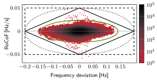
Figure 1: Scatter plot of frequency and RoCoF data (one year of measurements in $1\text{\,}\mathrm{s}$ resolution) in the CE interconnection (courtesy of RTE France). The color of each dot gives the frequency of each observation.

Figure 1 shows measurements from the continental European interconnection, covering one year in $1\text{\,}\mathrm{s}$ resolution. It is evident that the steepest RoCoF and largest frequency deviation do not occur at the same time, and $99.999\text{\,}\mathrm{\char 37\relax}$ of the data are contained in the green solid ellipse. The scaled 1-, 2- and $\infty$-norm balls (black solid, dotted and dashed, respectively) are based on limits considered for normal system operation, namely $200\text{\,}\mathrm{mHz}$ frequency deviation and $10\text{\,}\mathrm{mHz}\text{\,}{\mathrm{s}}^{-1}$ RoCoF, and contain all but seven measurements. The scaled 1- and 2-norm balls contain almost all observations, suggesting that simultaneous provision of $\tilde{M}$ and $\tilde{K}$ does not contradict itself. In the following we will show that the constraint for $\tilde{K}$ and $\tilde{M}$ is the dual of the bounding norm in $(\omega,\dot{\omega})$ space.

We observe that the constraint (15) is tight if $\omega_{k}$, $\dot{\omega}_{k}$ have the same sign. Henceforth, we will drop the absolute value. We express $\tilde{K}$ as a function of $\tilde{M}$, $\omega$ and $\dot{\omega}$:

$$\tilde{K}(\tilde{M},\omega,\dot{\omega})\leq\frac{\bar{P}}{\omega}-\frac{\tilde{M}\dot{\omega}}{\omega}\quad.$$ (16)

Consider a set of observations $(\omega,\dot{\omega})$ contained in a scaled $p$-norm ball of size $c>0$ and with scaling factor $h>0$:

$$\left((h\omega_{k})^{p}+\dot{\omega}^{p}_{k}\right)^{-p} \leq c \forall k\quad.$$ (17)

Assume the constraint (15) is tight for $(\omega,\dot{\omega})$ pairs on the boundary $(h\omega)^{p}+\dot{\omega}^{p}=c^{p}$. Hence, we can write (16) as

$$\tilde{K}(\tilde{M},\omega)\leq\frac{1}{\omega}\left({\overline{P}}-\tilde{M}\left(c^{p}-(h\omega)^{p}\right)^{-p}\right)\quad.$$ (18)

Thus, for each $\omega$ there is a linear upper bound (18) in $(\tilde{M},\tilde{K})$ space, constraining the choice of $\tilde{K}$ depending on $\tilde{M}$. The limiting constraint on $\tilde{K}$ for a given $\tilde{M}$ can be found by minimizing the right-hand side of (18) with respect to $\omega$. Aside from critical points at $|\omega|=\infty$, we obtain the others by setting the derivative of the right-hand side of (18) to zero

$$-{\overline{P}}+(c^{p}-(h\omega)^{p})^{q}c^{p}\tilde{M}=0$$ (19)

with $q=\frac{p}{p-1}$. After solving (19) for $\omega$, substituting the solution in (16), and after some reformulations, we arrive at

$$\left(\frac{\tilde{K}}{h}\right)^{q}+\tilde{M}^{q}=\left(\frac{{\overline{P}}}{c}\right)^{q}\quad.$$ (20)

Hence, $\tilde{K}$ and $\tilde{M}$ are bounded by the dual norm of (17).

Figure 2: Bounding boxes on reserve provision resulting from Figure 1, for a unit with $1\text{\,}\mathrm{p.u.}$

Figure 2 is a map of the $(\omega,\dot{\omega})$ space from Figure 1 into $(\tilde{M},\tilde{K})$ space, and with the limits from Figure 1 $h$ is $\frac{1}{20}$. Each data point in $(\omega,\dot{\omega})$ becomes a constraint in $(\tilde{M},\tilde{K})$ and the scaled $\infty$-, 2- and 1-norms translate to scaled 1-, 2- and $\infty$-norms, respectively. Of the three norms, we choose the scaled 1-norm in $(\omega,\dot{\omega})$-space which gives the best fit (like the other norms, it is only violated by few outliers) and which results in a linear and local box-constraint in $(\tilde{M},\tilde{K})$ space,

$$\begin{bmatrix}\tilde{K}/h\\ \tilde{M}\end{bmatrix} \leq\begin{bmatrix}{\overline{P}}\\ {\overline{P}}\end{bmatrix}\quad,$$ (21)

which is suitable for efficient linear program formulations.

IV Computation of gradient descent directions

Our inertia placement algorithm (presented formally in Section V) searches for parameters $\tilde{K}$, $\tilde{M}$ to optimize damping ratio, overshoot and RoCoF subject to constraints. Hence, we need the gradient or sensitivity of these performance indices with respect to these parameters. The following subsections describe how to compute or approximate these.

IV-A Computation of the sensitivity of the damping ratio

The sensitivity of the damping ratio (8) with respect to $\alpha$ is

$$\mathrm{D}_{\alpha}\zeta^{(i)}=\omega^{(i)}\frac{\left(\sigma^{(i)}\mathrm{D}_{\alpha}\omega^{(i)}-\omega^{(i)}\mathrm{D}_{\alpha}\sigma^{(i)}\right)}{\left((\sigma^{(i)})^{2}+(\omega^{(i)})^{2}\right)^{\frac{3}{2}}}\quad,$$ (22)

where the eigenvalue derivatives are obtained from [19] as

$$\mathrm{D}_{\alpha}\lambda^{(i)} =\bm{u}^{(i)\intercal}(\mathrm{D}_{\alpha}\bm{A})\bm{v}^{(i)}\quad.$$ (23)

IV-B Computation of the overshoot and its sensitivity

To find the overshoot (13), we use the Newton method to search for an extremum of the step response $\bm{y}(\bm{t}_{\mathrm{S}})$

$$\bm{t}_{\mathrm{S}}^{\nu+1} =\bm{t}_{\mathrm{S}}^{\nu}-\left.\left(\mathrm{D}_{t}\bm{y}\oslash\mathrm{D}^{2}_{t}\bm{y}\right)\right|_{\bm{t}=\bm{t}_{\mathrm{S}}^{\nu}}\quad,$$ (24)

with the n-th derivatives of (9) given by

$$\left.\mathrm{D}^{n}_{t}\bm{y}\right|_{\bm{t}} =-\sum\nolimits\nolimits_{i}(\lambda^{(i)})^{(n-1)}\bm{r}^{(i)}\!\odot\mathrm{e}^{\lambda^{(i)}\bm{t}}\quad,$$ (25)

and where $\odot$ and $\oslash$ denote the element-wise (Hadamard) multiplication and division. As $\nu\to\infty$, we obtain the (local) extremum $\bm{y}(\bm{t}_{\mathrm{S}})$ at $\bm{t}_{\mathrm{S}}^{\nu}\to\bm{t}_{\mathrm{S}}$. Since there may be multiple extrema, one needs a good starting point. Gridding the step response and starting from the largest point found leads to the correct extremum if the grid is chosen sufficiently small, e.g., twice the frequency of the highest mode frequency. If an estimate of $\bm{t}_{\mathrm{S}}$ is available, e.g., from a previous placement iteration, it can be used to initialize the Newton search.

It is quite involved to find the sensitivity of the overshoot with respect to $\alpha$: while it is easy to compute the change of the step response with respect to $\alpha$ given a fixed $\bm{t}$, the time of the overshoot $\bm{t}_{\mathrm{S}}$ is also a function of $\alpha$. Hence, simply taking $\left.\mathrm{D}_{\alpha}y\right|_{\bm{t}_{\mathrm{S}}}$ is incorrect. The correct derivative is

$$\mathrm{D}_{\alpha}\bm{S}=\sum\nolimits\nolimits_{i}\Bigg{[}\mathrm{D}_{\alpha}\frac{\bm{r}^{(i)}}{\lambda^{(i)}}\odot\left(1-\mathrm{e}^{\lambda^{(i)}\bm{t}_{\mathrm{S}}}\right)-\\ \frac{\bm{r}^{(i)}}{\lambda^{(i)}}\odot\left(\left(\mathrm{D}_{\alpha}\lambda^{(i)}\right)\bm{t}_{\mathrm{S}}+\lambda^{(i)}\mathrm{D}_{\alpha}\bm{t}_{\mathrm{S}}\right)\odot\mathrm{e}^{\lambda^{(i)}\bm{t}_{\mathrm{S}}}\Bigg{]}$$ (26)

which includes the derivative of the residues, the derivative of the eigenvalues, and the derivative of the peak time.

The derivative of the residues $\bm{r}^{(i)}$ is given by

$$\mathrm{D}_{\alpha}\bm{r}^{(i)} =\bm{C}\mathrm{D}_{\alpha}\left(\bm{v}^{(i)}\bm{u}^{(i)\intercal}\right)\bm{B}$$ (27)

$$\mathrm{D}_{\alpha}\frac{\bm{r}^{(i)}}{\lambda^{(i)}} =\frac{\left(\mathrm{D}_{\alpha}\bm{r}^{(i)}\right)\lambda^{(i)}-\bm{r}^{(i)}\mathrm{D}_{\alpha}\lambda^{(i)}}{(\lambda^{(i)})^{2}}\quad,$$ (28)

where $\mathrm{D}_{\alpha}\left(\bm{v}^{(i)}\bm{u}^{(i)\intercal}\right)$ can be computed as follows [19, 12]:

$$\mathrm{D}_{\alpha}\left(\bm{v}^{(i)}\bm{u}^{(i)\intercal}\right) =\mkern-9.0mu\sum\nolimits\nolimits_{j\in\mathcal{N}\setminus i}\mkern-6.0mu\left[\bm{v}^{(j)}c_{ij}^{\alpha}\bm{u}^{(i)\intercal}-\bm{v}^{(i)}c_{ji}^{\alpha}\bm{u}^{(j)\intercal}\right]$$ (29)

$$c_{ij}^{\alpha} =\frac{\bm{u}^{(j)\intercal}(\mathrm{D}_{\alpha}\bm{A})\bm{v}^{(i)}}{\left(\lambda^{(i)}-\lambda^{(j)}\right)}\quad i\neq j\quad.$$ (30)

Note that for the correct value of $c_{ij}^{\alpha}$ we used the normalization (12). Observe that the term $\lambda^{(i)}-\lambda^{(j)}$ is zero for double eigenvalues. While these usually do not occur in power systems unless the system is perfectly symmetric, one should ensure that the system at hand is well posed.

The derivative of the peak time $\bm{t}_{\mathrm{S}}$ cannot be exactly computed, as $\bm{t}_{\mathrm{S}}$ is found with the Newton method. We use as an approximation the derivative of the Newton update (24)

$$\mathrm{D}_{\alpha}\bm{t}_{\mathrm{S}}\approx-\mathrm{D}_{\alpha}\left(\mathrm{D}_{t}\bm{y}\oslash\mathrm{D}^{2}_{t}\bm{y}\right)\\ =-\Big{(}\left[\left(\mathrm{D}_{\alpha}\mathrm{D}_{t}\bm{y}\right)\odot\mathrm{D}^{2}_{t}\bm{y}-\mathrm{D}_{t}\bm{y}\odot\left(\mathrm{D}_{\alpha}\mathrm{D}^{2}_{t}\bm{y}\right)\right]\oslash\\ \left.\oslash\left[\mathrm{D}^{2}_{t}\bm{y}\odot\mathrm{D}^{2}_{t}\bm{y}\right]\Big{)}\right|_{\bm{t}=\bm{t}_{\mathrm{S}}},$$ (31)

for which we need (25) and the derivatives of the step response with respect to $\alpha$ explicitly given by:

$$\mathrm{D}_{\alpha}\mathrm{D}_{t}\bm{y} =-\sum\nolimits_{i}\left[\mathrm{D}_{\alpha}\bm{r}^{(i)}+\bm{r}^{(i)}\!\odot\bm{t}\mathrm{D}_{\alpha}\lambda^{(i)}\right]\odot\mathrm{e}^{\lambda^{(i)}\bm{t}}$$ (32)

$$\mathrm{D}_{\alpha}\mathrm{D}^{2}_{t}\bm{y} =-\sum\nolimits_{i}\left[\mathrm{D}_{\alpha}\bm{r}^{(i)}\lambda^{(i)}+\bm{r}^{(i)}\mathrm{D}_{\alpha}\lambda^{(i)}+\right.$$

$$\left.+\bm{r}^{(i)}\!\odot\bm{t}\lambda^{(i)}\mathrm{D}_{\alpha}\lambda^{(i)}\right]\odot\mathrm{e}^{\lambda^{(i)}\bm{t}}\quad.$$ (33)

Observe that the approximation (31) is actually exact if the Newton method converges in one step. This is the case if $\bm{y}$ is a quadratic function. In our case, $\bm{y}$ consists of sinusoidal functions, and we assume to be at an extremum for the previous parameter value $\alpha$ where sinusoidal functions are described up to fourth order terms by quadratic functions. Hence, in practice, we observe that the approximation (31) performs very well; see later simulations in Section VII.

IV-C Computation of the RoCoF and its sensitivity

The RoCoF $\bm{R}$ (13) is also found using the Newton method

$$\bm{t}_{\mathrm{R}}^{\nu+1} =\bm{t}_{\mathrm{R}}^{\nu}-\left.\left(\mathrm{D}^{2}_{t}\bm{y}\oslash\mathrm{D}^{3}_{t}\bm{y}\right)\right|_{\bm{t}=\bm{t}_{\mathrm{R}}^{\nu}}\quad,$$ (34)

where $\bm{t}_{\mathrm{R}}^{\nu}\to\bm{t}_{\mathrm{R}}$ as $\nu\to\infty$. and $\bm{R}=\bm{y}(\bm{t}_{\mathrm{R}})$.

To find the sensitivity of $\bm{R}$ with respect to $\alpha$ we use the same approach as for the sensitivity of the overshoot $\mathrm{D}_{\alpha}\bm{S}$; see equations (26) to (33). The RoCoF sensitivity is

$$\mathrm{D}_{\alpha}\bm{R}=-\sum\nolimits_{i}\Bigg{[}\mathrm{D}_{\alpha}\bm{r}^{(i)}+\bm{r}^{(i)}\!\odot\bm{t}_{\mathrm{R}}\mathrm{D}_{\alpha}\lambda^{(i)}+\\ +\bm{r}^{(i)}\!\odot\left(\mathrm{D}_{\alpha}\bm{t}_{\mathrm{R}}\right)\lambda^{(i)}\Bigg{]}\odot\mathrm{e}^{\lambda^{(i)}\bm{t}_{\mathrm{R}}}\quad,$$ (35)

using (23) and (27). The sensitivity of $\bm{t}_{\mathrm{R}}$ is approximated by the derivative of the RoCoF Newton update step,

$$\mathrm{D}_{\alpha}\bm{t}_{\mathrm{R}}\approx-\mathrm{D}_{\alpha}\left(\mathrm{D}^{2}_{t}\bm{y}\oslash\mathrm{D}^{3}_{t}\bm{y}\right)\\ =-\Big{(}\left[\left(\mathrm{D}_{\alpha}\mathrm{D}^{2}_{t}\bm{y}\right)\odot\mathrm{D}^{3}_{t}\bm{y}-\mathrm{D}^{2}_{t}\bm{y}\odot\left(\mathrm{D}_{\alpha}\mathrm{D}^{3}_{t}\bm{y}\right)\right]\oslash\\ \left.\oslash\left[\mathrm{D}^{3}_{t}\bm{y}\odot\mathrm{D}^{3}_{t}\bm{y}\right]\Big{)}\right|_{\bm{t}=\bm{t}_{\mathrm{R}}},$$ (36)

with (25), (33) and

$$\mathrm{D}_{\alpha}\mathrm{D}^{3}_{t}\bm{y}=-\sum\nolimits_{i}\Big{[}\mathrm{D}_{\alpha}\bm{r}^{(i)}\left(\lambda^{(i)}\right)^{2}+2\bm{r}^{(i)}\lambda^{(i)}\mathrm{D}_{\alpha}\lambda^{(i)}+\\ +\bm{r}^{(i)}\!\odot\bm{t}\left(\lambda^{(i)}\right)^{2}\mathrm{D}_{\alpha}\lambda^{(i)}\Big{]}\odot\mathrm{e}^{\lambda^{(i)}\bm{t}}.$$ (37)

V Optimal inertia placement algorithm

In the following we present the objectives of our synthetic inertia allocation optimization (Section V-A), pose the program in a general form (Section V-B), and a sequential linear programming approach to solve it (Section V-C).

V-A Formulation of optimization objectives

We aim to co-optimize three metrics, namely the damping ratio $\zeta$, the overshoot $\bm{S}$ and the RoCoF $\bm{R}$.

To maximize the smallest $\zeta$, we introduce the variable $\zeta^{\mathrm{min}}$

$$\zeta^{\mathrm{min}} \leq\zeta^{(i)} \forall\{i|\omega^{(i)}>0\}\quad,$$ (38a)

and consider the cost term

$$\min\nolimits_{\alpha}-c^{\zeta}\zeta^{\mathrm{min}}$$ (38b)

with positive $c^{\zeta}$, pushing $\zeta^{\mathrm{min}}$ against the smallest $\zeta^{(i)}$.

Similarly, to minimize the steepest RoCoF, $R_{\infty}$, we consider the cost term

$$\min\nolimits_{\alpha}c^{\mathrm{R}}R_{\infty}$$ (39a)

with positive parameter $$c^{\mathrm{R}}$$ and subject to

$$R_{\infty} \geq|(\bm{R})_{ij}| \forall i,j\leavevmode\nobreak\ .$$ (39b)

Analogous constraints and costs are used for the overshoot $\bm{S}$.

V-B Inertia and damping placement algorithm

We pose the optimal synthetic inertia and damping placement problem as a multi-objective optimization problem:

$$\min\nolimits_{\alpha}-c^{\zeta}\zeta^{\mathrm{min}}+c^{\mathrm{R}}R_{\infty}+c^{\mathrm{S}}S_{\infty}$$ (40a)

s.t. $$\underline{\zeta} \leq\zeta^{(i)} \forall\{i|\omega^{(i)}>0\}$$ (40b)

$$\underline{\bm{R}} \leq(\bm{R})_{ij}\leq\overline{\bm{R}} \forall i,j$$ (40c)

$$\underline{\bm{S}} \leq(\bm{S})_{ij}\leq\overline{\bm{S}} \forall i,j$$ (40d)

$$0 \leq\tilde{K}_{v}/h\leq{\overline{P}}_{v} \forall v$$ (40e)

$$0 \leq\tilde{M}_{v}\leq{\overline{P}}_{v} \forall v$$ (40f)

The cost function (40a) combines the three-level objective discussed in Section V-A. The constraints (40b) to (40d) put strict bounds on all damping ratios, RoCoFs and overshoots. Constraints (40e) and (40f) define bounds on synthetic inertia and damping provision according to Section III; confer (21).

Thus, our inertia and damping allocation problem (40) combines system-level objectives, such as the damping ratio, together with explicit time-domain criteria and strict constraints on RoCoF, overshoot, and device-level power limits.

V-C Sequential linear programming approach

The optimization problem (40) is non-linear, typically large-scale for the considered system, and highly non-convex. Hence we use a sequential linear programming approach iterating over parameters $\alpha$ until we reach a local optimum.

At each iteration a first-order (linear) approximation of (40) is obtained as follows. Given values $\alpha^{\nu}$, $\zeta_{\nu}^{(j)}$, $\bm{R}^{\nu}$, and $\bm{S}^{\nu}$ at iteration $\nu$, the performance metrics are then updated by means of the sensitivities derived in Section IV as

$$\tilde{\zeta}_{\nu+1}^{(j)} =\zeta_{\nu}^{(j)}+\sum\nolimits_{\forall\alpha}\mathrm{D}_{\alpha}\zeta_{\nu}^{(j)}\Delta\alpha^{\nu} \forall\{j|\omega^{(j)}>0\}$$ (41a)

$$\tilde{\bm{R}}^{\nu+1} =\bm{R}^{\nu}+\sum\nolimits_{\forall\alpha}\mathrm{D}_{\alpha}\bm{R}^{\nu}\Delta\alpha^{\nu}$$ (41b)

$$\tilde{\bm{S}}^{\nu+1} =\bm{S}^{\nu}+\sum\nolimits_{\forall\alpha}\mathrm{D}_{\alpha}\bm{S}^{\nu}\Delta\alpha^{\nu}\quad,$$ (41c)

with $\alpha^{\nu}+\Delta\alpha^{\nu}=\alpha^{\nu+1}$, $\Delta\alpha^{\nu}$ being a (time-varying) step-size, and $\zeta_{\nu}^{(j)}=\zeta(\alpha^{\nu})$, $\bm{R}^{\nu}=\bm{R}(\alpha^{\nu})$ and $\bm{S}^{\nu}=\bm{S}(\alpha^{\nu})$.

The left-hand terms in (41) are first-order approximations when $\alpha^{\nu}$ is updated to $\alpha^{\nu+1}$. By setting $\tilde{\zeta}_{\nu+1}^{(j)}=\zeta^{(j)}$, $\tilde{\bm{R}}^{\nu+1}=\bm{R}$ and $\tilde{\bm{S}}^{\nu+1}=\bm{S}$ in (40), we obtain a linear programming formulation.

Updates and limits of the step size: As (41) are only locally valid linearizations, we need to limit the step size $\Delta\alpha^{\nu}$ as

$$-\Delta\alpha^{\mathrm{max}} \leq\Delta\alpha^{\nu}\leq\Delta\alpha^{\mathrm{max}} \forall\alpha\quad,$$ (42)

where $\Delta\alpha^{\mathrm{max}}>0$. After each iteration, the updated system matrix $\bm{A}(\alpha^{\nu+1})$ and performance indices $\zeta$, $\bm{S}$ and $\bm{R}$ are computed. If they show an improvement, $\alpha^{\nu+1}$ is kept. Otherwise, the previous value $\alpha^{\nu}$ is used, and the step size $\Delta\alpha^{\mathrm{max}}$ is halved for all $\Delta\alpha$ that hit $\Delta\alpha^{\mathrm{max}}$.

Iterations: Due to the mismatch between the linearly approximation $\tilde{\bm{R}}^{\nu+1}$ and the true value $\bm{R}(\alpha^{\nu+1})$, the new starting point $\bm{R}(\alpha^{\nu+1})$ may violate the constraint (40c). To ensure feasibility, we add a slack variable to this constraint,

$$\underline{\bm{R}} \leq(\bm{R})_{ij}^{\nu+1}-\epsilon^{\mathrm{R}}_{ij}\leq\overline{\bm{R}} \forall i,j$$ (43a)

The slack variable is only added if the starting point of the iteration is infeasible

$$0 \leq\epsilon^{\mathrm{R}}_{ij} \forall\{i,j|(\bm{R})_{ij}^{\nu}>\overline{\bm{R}}\}$$ (43b)

$$0 =\epsilon^{\mathrm{R}}_{ij} \forall\{i,j|(\bm{R})_{ij}^{\nu}\in[\underline{\bm{R}},\overline{\bm{R}}]\}$$ (43c)

$$0 \geq\epsilon^{\mathrm{R}}_{ij} \forall\{i,j|(\bm{R})_{ij}^{\nu}<\underline{\bm{R}}\}$$ (43d)

and the slack is penalized with a large cost term $$c^{\epsilon\mathrm{R}}>0$$ as

$$\min\nolimits_{\alpha}\sum\nolimits_{d,b}c^{\epsilon\mathrm{R}}\epsilon^{\mathrm{R}}_{ij}\quad.$$ (43e)

The same approach is used to ensure feasibility of $\zeta$ and $\bm{S}$.

Stopping criterion: The algorithm terminates after a fixed number of iterations, when the performance improvement is smaller than a threshold, or when the step size for all $\alpha$ is below a threshold.

V-D Considerations on numerics

The main computational effort at each iteration of our algorithm is to obtain all eigenvalues, eigenvectors and sensitivities. Clearly, this is computationally burdensome for large systems, but the scaling is reasonable as shown below.

Of the needed computations, the derivatives of the eigenvectors have the worst scaling. For each $\alpha$, we need to compute all $N$ eigenvector derivatives. For each eigenvector derivative, we need $c_{kj}^{\alpha}$ which has dimension $\mathbb{R}^{N\times N}$. Assuming $N^{A}$ parameters, this leads to $N_{A}\,N^{3}$ entries. By exploiting the structure of our problem, we can significantly reduce the number of entries: while we need all eigenvector derivatives, we only need the entries that correspond to non-zero entries in $\bm{B}$ and $\bm{C}$. These scale with the number of disturbances $N_{B}$ and observed frequencies $N_{C}$, giving a scaling of $\mathcal{O}(N\,N_{A}\,N_{B}\,N_{C})$. The dimensions $N_{B}$ and $N_{C}$ are much smaller than $N$. Additionally, if we change the model and add some states while keeping the number of disturbances and outputs constant, the computational effort for the eigenvector derivatives scales linearly instead of cubic. This allows much more freedom on modeling choices.

Computation of the overshoot $\bm{S}$ and RoCoF $\bm{R}$ matrices, both in $\mathbb{R}^{D\times B}$, via the iterative Newton method, is comparably efficient. While at the first iteration of the overall placement algorithm, we grid the system to find the global extrema, we use the previous $\bm{t}_{\mathrm{S}}$ and $\bm{t}_{\mathrm{R}}$ as starting points for the Newton method in the next iteration and compute all $\bm{t}_{\mathrm{S}}$ and $\bm{t}_{\mathrm{R}}$ in parallel. With this implementation, it takes usually only few Newton iterations to find the values of $\bm{S}$ and $\bm{R}$.

V-E Alternative optimization problem formulations

In the following, we briefly discuss a few alternative formulations of the optimal inertia and damping allocation problem (40) which are useful in other scenarios.

Power capacity: Previously, we assumed the power capacity ${\overline{P}}_{v}$ of each inertia device to be fixed. This renders the program (40) a scheduling problem answering how much of the available inertia at a certain node should be used, depending on the expected system state. Alternatively, we can make ${\overline{P}}_{v}$ a decision variable, rendering the program (40) a planning problem. If a fixed amount of inertia-devices is to be placed in the system, one would add the budget constraint

$$\sum\nolimits{\overline{P}}_{v} \leq P^{\mathrm{bdg}}\quad.$$ (44)

Finally, $P^{\mathrm{bdg}}$ can be itself be a decision variable as well with an associated cost that reflects the investment cost of synthetic inertia devices in a planning program.

Average performance: Instead of optimizing and limiting the worst-case performance as in (40), we could also optimize the average performance objective

$$\min\limits_{\alpha^{\nu+1}}-c^{\zeta}\sum\limits_{j}\zeta_{\nu}^{(j)}+c^{\mathrm{S1}}\sum\limits_{i,j}(\bm{S})_{ij}+c^{\mathrm{R1}}\sum\limits_{i,j}(\bm{R})_{ij}\quad.$$ (45)

Such an average objective allows to trade off damping, RoCoF and overshoot between different buses in the system.

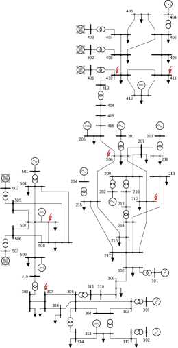
Figure 3: Topology of the test system.

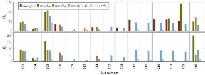
Figure 4: Synthetic inertia and damping distribution with different cost functions

VI Description of the test case

We use a modified version of the Australian 14 generator system as a test case to illustrate the utility of our synthetic inertia and damping placement algorithm.

Base system: The Australian system [15], see Figure 3, consists of 14 generators and 59 buses. Gibbard and Vowles describe six load cases, of which we chose the heavy loading case. The system consists of five areas connected in a string-like layout. The main demand, Melbourne and Sydney, is in the middle of the system, while significant generation is located in all areas including the two far ends of the system. We use the AVR and PSS parameters given in [15].

The model is extended with motor loads and load damping. We assume $10\text{\,}\mathrm{\char 37\relax}$ of the load to be from motors with an inertia of $1.5\text{\,}\mathrm{s}$. Load damping is set to $2.5\text{\,}\mathrm{p.u.}$, and dynamic loads are behind an $0.1\text{\,}\mathrm{p.u.}$ inductance [20].

Low-inertia case study: For the case study, we remove five generators from the system, namely 401, 402, 403, 502 and 503. These are generators in the West and North ends of the system, where there is abundant wind and solar resources, respectively, and which are likely areas for RES deployment in Australia. We assume renewable generation to have a grid-following maximum power-point tracking control feeding constant active and reactive power into the system.

Disturbances: We model disturbances as sudden load increases of $250\text{\,}\mathrm{MW}$ at some load buses, namely 206, 212, 307, 410, 411 and 508. We chose such generic faults as they do not affect the $\bm{A}$-matrix of the system.

Monitored frequencies: To identify the effect of removing generators and adding synthetic inertia, we monitor the frequency $\omega^{\mathrm{G}}$ at all remaining conventional generators and compute $\zeta$, $\bm{R}$ and $\bm{S}$ at these buses.

Synthetic inertia and damping budget: For better comparability with the initial system, we allow the same amount of inertia to be added to the system as is lost due to generator removal. In system base this amounts to an inertia budget $\tilde{M}^{\mathrm{bdg}}$ of $475\text{\,}\mathrm{s}$, which depending on the largest (expected) ROCOF translates to the power budget

$$P^{\mathrm{bdg}}=\tilde{M}^{\mathrm{bdg}}\max|\dot{\omega}|\quad.$$ (46)

Finally, the choice of $h$ in (40e) is a relevant design parameter, which traces back to the observed system dynamics in (17). The observed frequency and ROCOF in the CE system suggested $h=\frac{1}{20}$, typical settings for protection relays are at $2\text{\,}\mathrm{Hz}$ and $0.5\text{\,}\mathrm{Hz}\text{\,}{\mathrm{s}}^{-1}$, suggesting $h=\frac{1}{4}$, while simulations of the test system give higher ROCOF then frequency excursions, suggesting $h\approx 3$. We have chosen $h=1$ but recommend to assess this carefully for the system under consideration.

VII Results

In this section we compare different cost functions for our placement algorithm. We test five approaches: 1) maximizing worst-case damping ratio, 2) minimizing worst-case RoCoF, 3) minimizing worst-case overshoot, 4) co-optimizing average overshoot and RoCoF as in (45), and 5) penalizing the expenditure of synthetic inertia and damping; see Section V-E.

We first discuss and compare the first four case studies. Figure 4 shows the allocation of synthetic inertia depending on each of the four cost functions. It is immediately evident that the different cost functions lead to significantly different inertia distributions. Table I gives a comparison and cross-validation of the results for these four cases. As performance indices we use the worst-case metrics $\zeta^{\mathrm{min}}$, $R_{\infty}$ and $S_{\infty}$; the total allocation of inertia and of damping, $\sum\nolimits\tilde{M}$ and $\sum\nolimits\tilde{K}$; and the mean RoCoF and mean overshoot, $R_{1}$ and $S_{1}$. The optimal placement of inertia outperforms the initial allocation and helps to alleviate the loss of generators. Depending on the cost function, the performance metrics are affected in quite different ways. Also, the inertia budget is never fully utilized, hinting at the fact that with optimal placement, actually little synthetic inertia is needed. We also observe that each performance metric is lowest when it is considered in the cost function, suggesting that the results are plausible.

Table I: Comparison of results

Metric	$\zeta^{\mathrm{min}}$	$R_{\infty}$	$S_{\infty}$	$\sum\nolimits\tilde{M}$	$\sum\nolimits\tilde{K}$	$R_{1}$	$S_{1}$
	%	[mHz/s]	[mHz]	[pu]	[pu]	[mHz/s]	[mHz]
initial system	$18.6414$	$193.108$	$56.4528$	–	–	$30.2605$	$20.0082$
low inertia	$19.1432$	$395.756$	$98.2757$	–	–	$34.9901$	$18.9289$
$\min\nolimits-\zeta^{\mathrm{min}}$	$19.2386$	$378.861$	$90.1813$	$310.717$	$6.446\,73$	$30.7658$	$18.1864$
$\min\nolimits S_{\infty}$	$14.9994$	$96.2151$	$27.3695$	$417.48$	$237.665$	$21.4256$	$12.0297$
$\min\nolimits R_{\infty}$	$14.9999$	$94.0839$	$28.4442$	$429.313$	$163.326$	$22.8881$	$15.5199$
$\min\nolimits S_{1}+R_{1}$	$17.0341$	$96.247$	$27.5439$	$464.629$	$438.961$	$18.8276$	$10.7923$
$\min\nolimits\sum\nolimits{\overline{P}}_{v}$	$15.9$	$95.9$	$30.0$	$87.6$	$63.3$	$24.5$	$15.7$

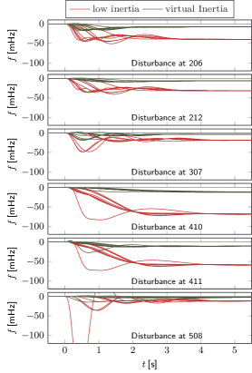
Figure 5: Step response of linearized system. Low inertia (red) and optimal inertia placement (green) with cost function 4).

1) Optimizing the damping ratio $\zeta^{\max}$: To maximize the damping ratio, our allocation algorithm places inertia mainly in the center of the system and places very little damping.

2) Minimizing the largest overshoot $S_{\infty}$: While the largest overshoot occurs at bus 501, to minimize $S_{\infty}$ inertia and damping are placed in Area 4, and only some in Area 5. It seems that already little additional virtual inertia in Area 5 suffices to alleviate overshoot issues.

3) Minimizing the largest RoCoF $R_{\infty}$: The largest RoCoF is found at bus 501, after a disturbance at bus 508. Accordingly, to minimize the RoCoF most inertia as well as some damping are allocated in Area 5. Incidentally, this is the area of a recent black-out in the grid, blamed on insufficient fault-ride-through capabilities of wind generation [16].

4) Co-optimizing the overshoot and the RoCoF: Penalizing the average overshoot and RoCoF as in (45) leads to a very even distribution of damping and inertia at the outer areas 2, 4 and 5. It also leads to $R_{\infty}$ and $S_{\infty}$ that are close to the ones achieved in the two previous approaches. It seems that such a cost function taking into account all frequencies and not only the worst excursions gives the most benign system behaviour. Figure 5 shows the step response with this distribution compared to the low-inertia case.

5) Minimal inertia expenditure: Finally, we minimize the use of synthetic inertia and damping, by making $P^{\mathrm{bdg}}$ in (44) a decision variable, while keeping the RoCoF, overshoot and damping ratio in bounds of $100\text{\,}\mathrm{mHz}\text{\,}{\mathrm{s}}^{-1}$, $30\text{\,}\mathrm{mHz}$ and $15\text{\,}\mathrm{\char 37\relax}$. Perhaps surprisingly, we can reduced synthetic inertia requirements by a factor five within the imposed constraints.

VIII Conclusion

This paper presented an algorithm for optimal inertia placement with explicit time-domain constraints. A case study on the Australian grid shows the applicability to realistic power system models. With that in mind, the algorithm can be a valuable tool in short and long term planning of power system stability and inertia deployment.

The approach can be easily extended to answer more detailed questions. For example, one can extend the modeling framework to include HVDC lines that emulate inertia by transferring energy from one part of the system to another.

Another direction of research is valuation of inertia provision. The optimization problem gives rise to a notion of location marginal inertia prices in line with traditional locational marginal pricing, as argued in [21].

References

- [1] A. Ulbig, T. S. Borsche, and G. Andersson, “Impact of Low Rotational Inertia on Power System Stability and Operation,” in Proceedings of the 19th IFAC World Congress, Cape Town, aug 2014, pp. 7290–7297.
- [2] P. Tielens and D. Van Hertem, “The relevance of inertia in power systems,” Renewable and Sustainable Energy Reviews, vol. 55, pp. 999–1009, 2016.
- [3] EirGrid and Soni, “DS3: System Services Review TSO Recommendations,” EirGrid, Tech. Rep., 2012.
- [4] ERCOT, “Future Ancillary Services in ERCOT,” ERCOT, Tech. Rep., 2013.
- [5] “Challenges and opportunities for the nordic power system,” statnett, fingrid, energinet.dk, svenska kraftnätt, Tech. Rep., Aug 2016.
- [6] H. Bevrani, T. Ise, and Y. Miura, “Virtual synchronous generators: A survey and new perspectives,” Intl. Journal of Electrical Power & Energy Systems, vol. 54, Jan. 2014.
- [7] D. Gross, S. Bolognani, B. K. Poolla, and F. Dörfler, “Increasing the resilience of low-inertia power systems by virtual inertia and damping,” in Bulk Power Systems Dynamics and Control Symposium (IREP), 2017, to appear.
- [8] E. Rakhshani, D. Remon, A. M. Cantarellas, and P. Rodriguez, “Analysis of derivative control based virtual inertia in multi-area high-voltage direct current interconnected power systems,” IET Generation, Transmission & Distribution, vol. 10, no. 6, pp. 1458–1469, 2016.
- [9] B. K. Poolla, S. Bolognani, and F. Dörfler, “Placing rotational inertia in power grids,” in American Control Conference (ACC), 2016. IEEE, 2016, pp. 2314–2320.
- [10] M. Pirani, J. W. Simpson-Porco, and B. Fidan, “System-theoretic performance metrics for low-inertia stability of power networks,” arXiv preprint arXiv:1703.02646, 2017.
- [11] A. Mesanovic, U. Münz, and C. Hyde, “Comparison of H∞ , H2 , and pole optimization for power system oscillation damping with remote renewable generation,” in IFAC Workshop on Control of Transmission and Distribution Smart Grids - CTDSG’16, Prague, 2016.
- [12] T. S. Borsche, T. Liu, and D. J. Hill, “Effects of Rotational Inertia on Power System Damping and Frequency Transients,” in 54th IEEE Conference on Decision and Control (CDC), Osaka, 2015.
- [13] C. D. Vournas and B. C. Papadias, “Power system stabilization via parameter optimization-application to the Hellenic interconnected system,” IEEE Transactions on Power Systems, vol. 2, no. 3, pp. 615–622, 1987.
- [14] B. K. Poolla, D. Gross, T. Borsche, S. Bolognani, and F. Dörfler, “Virtual inertia placement in electric power grids,” in Energy Markets and Responsive Grids, J. Stoustrup, Ed., 2017.
- [15] M. Gibbard and D. Vowles, “Simplified 14-Generator Model of the South East Australian Power System, Revision 4,” Tech. Rep. June, 2014.
- [16] AEMO, “Update Report - Black System Event in South Australia on 28 September 2016,” Tech. Rep., 2016.
- [17] A. R. Bergen and D. J. Hill, “A structure preserving model for power system stability analysis,” IEEE Transactions on Power Apparatus and Systems, vol. PAS-100, no. 1, pp. 25–35, 1981.
- [18] F. Dörfler and F. Bullo, “Kron reduction of graphs with applications to electrical networks,” IEEE Transactions on Circuits and Systems I: Regular Papers, vol. 60, no. 1, pp. 150–163, January 2013.
- [19] D. V. Murthy and R. T. Haftka, “Derivatives of eigenvalues and eigenvectors of a general complex matrix,” International Journal for Numerical Methods in Engineering, vol. 26, pp. 293–311, 1988.
- [20] P. Kundur, Power System Stability and Control, 1st ed., N. J. Bau and M. G. Lauby, Eds. McGraw-Hill Professional, 1994.
- [21] T. S. Borsche, “Impact of demand and storage control on power system operation and dynamics,” Ph.D. dissertation, ETH Zürich, Feb 2016.