A higher-order Skyrme model

Abstract

We propose a higher-order Skyrme model with derivative terms of eighth, tenth and twelfth order. Our construction yields simple and easy-to-interpret higher-order Lagrangians. We first show that a Skyrmion with higher-order terms proposed by Marleau has an instability in the form of a baby-Skyrmion string, while the static energies of our construction are positive definite, implying stability against time-independent perturbations. However, we also find that the Hamiltonians of our construction possess two kinds of dynamical instabilities, which may indicate the instability with respect to time-dependent perturbations. Different from the well-known Ostrogradsky instability, the instabilities that we find are intrinsically of nonlinear nature and also due to the fact that even powers of the inverse metric gives a ghost-like higher-order kinetic-like term. The vacuum state is, however, stable. Finally, we show that at sufficiently low energies, our Hamiltonians in the simplest cases, are stable against time-dependent perturbations.

1 Introduction

The Skyrme model Skyrme:1962vh ; Skyrme:1961vq is generally believed to describe low-energy QCD at large $N_{c}$ Witten:1983tw ; Witten:1983tx . It has also been derived directly from the QCD Lagrangian by means of partial bosonization Zaks:1985cv . As well known, it is not possible to perform a full bosonization in 3+1 dimensions and hence the latter reference is bosonizing only the phases of the fermions. The Skyrme model has also been derived in the Sakai-Sugimoto model Sakai:2004cn by considering the effective action for the zero mode. All these derivations of the Skyrme model include a kinetic term as well as the Skyrme term, which is fourth order in derivatives. Skyrme introduced the term Skyrme:1962vh ; Skyrme:1961vq in order to stabilize the soliton – the Skyrmion – from collapse, as otherwise is unavoidable due to Derrick’s theorem Derrick:1964ww . However, higher-order derivative corrections higher than fourth order are generally expected.

As expected in QCD and explicitly shown in the Sakai-Sugimoto model Sakai:2004cn , an infinite tower of vector mesons exist as one goes up in energy scales. For each of these massive vector mesons, one can obtain effective operators in a pure pion theory by integrating out the massive mesons. The interaction terms between the pions and the mesons yield new low-energy effective operators. The first higher-derivative correction to the Skyrme model is expected to be a sixth-order derivative term, see e.g. Adkins:1983nw ; Jackson:1985yz ; Marleau:1989fh ; Marleau:1990nh ; Marleau:1991jk ; Marleau:2000ia ; Adam:2010fg ; Adam:2010ds ; Gudnason:2013qba ; Gudnason:2014jga ; Gudnason:2014hsa ; Gudnason:2015nxa ; Gudnason:2016yix . Physically, it corresponds to integrating out the $\omega$-meson Adkins:1983nw ; Jackson:1985yz ; this can be seen from the phenomenological Lagrangian with the interaction describing the decay $\omega\to\pi^{+}\pi^{-}\pi^{0}$.

The sixth-order term – which we shall call the BPS-Skyrme term – recently caught interest due to its BPS properties when it is paired with a suitable potential Adam:2010fg ; Adam:2010ds ; Gudnason:2013qba ; Gudnason:2014jga ; Gudnason:2014hsa ; Gudnason:2015nxa ; Gudnason:2016yix . Here BPS simply means that the energy is proportional to the topological number – the Skyrmion number, $B$ – of the model. This is a desired feature in nuclear physics where binding energies are very small.

In principle, we expect infinitely many higher-derivative terms in the low-energy effective action. However, as each term is larger in canonical dimension, it necessarily has to be accompanied by a dimensional constant to the same power minus four. That constant is typically proportional to the mass of the state that was integrated out of the underlying theory. Therefore, as long as the energy scales being probed are much smaller than the lowest mass scale of a state that was integrated out, the higher-derivative expansion may make sense and thus converge.

Apart from a construction based on the hedgehog Ansatz by Marleau Marleau:1989fh ; Marleau:1990nh ; Marleau:1991jk ; Marleau:2000ia , no extensive studies on higher-derivative terms in 3+1 dimensions, higher than sixth order, has been carried out in the literature – to the best of our knowledge. Marleau considered a construction that yielded higher-order derivative corrections to the Skyrmion, but restricted in such a way as to give only a second-order equation of motion for the radial profile (chiral angle function) Marleau:1989fh ; Marleau:1990nh ; Marleau:1991jk ; Marleau:2000ia . When restricted to spherical symmetry, this construction gives stable profiles when certain stability criteria are satisfied Jackson:1991mt . Nevertheless, as we will show in Sec. 3, when relaxing the spherical symmetry, this construction becomes unstable. Longpré and Marleau later found that avoiding the instability was indeed difficult Longpre:2005fr ; Longpre:2007zz ; they proposed a stability criterion that, however, cannot be satisfied for a finite-order derivative Lagrangian without causing Derrick instability. We will propose our interpretation of the instability as well as why it occurs and show that to finite order, it cannot be cured (stabilized). The instability occurs if perturbations are independent of one spatial direction. In particular, one can contemplate a perturbation in form of a baby-Skyrmion string which can trigger a run-away instability. The reason behind the instability is basically the requirement of the radial direction to be special (that is, to obey only a second-order equation of motion, whereas the angular directions enjoy many more powers of derivatives). This loss of isotropy brings about the latter mentioned instability.

In this paper, we take the construction of higher-order derivative corrections to the next level. The spirit of our construction is similar to that behind the Skyrme term and the BPS-Skyrme term. Take the Skyrme term; it is fourth order in spacetime derivatives. The most general term with fourth-order derivatives will contain four time derivatives. The Skyrme term does not; it is constructed in such a way as to cancel the fourth-order derivatives in the $i$-th space or time direction and contains four spacetime derivatives only as a product of second-order derivatives in two different space or time directions; e.g. $(\partial_{x}\phi)^{2}(\partial_{y}\phi)^{2}$ or $(\partial_{t}\phi)^{2}(\partial_{x}\phi)^{2}$. Note that this is the minimal number of derivatives in the $i$-th direction (we will denote this number by $\delta$). Two derivatives in the $i$-th direction is, however, only possible for terms up to and including sixth-order in derivatives in 3 spatial dimensions or eighth-order in derivatives in 4 spacetime dimensions. We prove, however, that the latter term vanishes identically in the Skyrme model ($S^{3}$ target space). For eighth-, tenth- and twelfth-order derivative terms, the smallest number of derivatives in the $i$-th direction is four, i.e. $\delta=4$. That is, when we do not break isotropy.

Our construction is straightforward and yields positive-definite static energies for the systems. We find simple interpretations for the Lagrangians that we constructed. The eighth-order Lagrangian can be understood as the sum of the Skyrme-term squared and the kinetic term multiplied by the BPS-Skyrme term (the sixth-order term mentioned above). The tenth-order Lagrangian can be interpreted as the Skyrme term multiplied by the BPS-Skyrme term. Finally, the twelfth-order Lagrangian can be interpreted as the BPS-Skyrme term squared.

We successfully achieve manifest stability for static energy associated with the higher-order Lagrangians. However, in order to check that time-dependent perturbations cannot spoil this stability, we construct the corresponding Hamiltonians. The Hamiltonians, as well known, are important objects because they give rise to the Euler-Lagrange equations of motion (as the Lagrangians do) and because we do not have any explicit time dependence, they are conserved and thus can be associated with the total energy. Although the Hamiltonians do not suffer from the famous Ostrogradsky instability Ostrogradsky:1850 ; Woodard:2015zca (see also Ref. Pais:1950za ), their highly nonlinear nature induces nonlinearities in the conjugate momenta and hence in the Hamiltonians themselves which potentially may destabilize the systems and in turn their solitons. The dynamical instability we find is intrinsically different from the Ostrogradsky one, because we do not have two time derivatives acting on the same field, but simply large powers of one time derivative acting on one field (see Appendix B). This implies that we only have a single conjugate momentum for each field (as opposed to several as in Ostrogradsky’s Lagrangian) and there is no run-away associated with a linear conjugate momentum in the Hamiltonian. Nevertheless, our construction yields a nonlinear conjugate momentum which induces ghost-like kinetic terms. In particular, the terms containing fourth-order time derivatives are accompanied by two powers of the inverse metric, which thus acquires the wrong sign – this term therefore remains negative in the Hamiltonian. The other effect we find is also related to the nonlinearities of the higher-order derivative terms, namely, when a term has more than two time derivatives the SO(3,1) symmetry of the Lorentz invariants is not simply transformed to SO(4) invariants by the standard Legendre transform, but the latter SO(4) symmetry is broken. This breaking of the would-be SO(4) symmetry induces terms with both signs. This is also related to our construction producing “minimal” Lagrangians, i.e. terms that are as simple as possible in terms of eigenvalues of the strain tensor. Although we find the above dynamical instabilities in our Hamiltonians, we conjecture that the vacuum is stable.

Finally, we argue that the Hamiltonian intrinsically knows that it is a low-energy effective field theory and that the instabilities described above do not occur at leading order for time-dependent perturbations. We consider the simplest possible perturbation, i.e. exciting the translational zero mode, and associating the energy scale of said perturbation with a velocity. We find exact conditions for when the instability sets in and estimate the velocities for which the effective theory will break down. In all cases the critical velocities are of the order of about half the speed of light. Then we show that to leading order in the velocity squared, there is no instability of the Hamiltonians of eighth and twelfth order.

The paper is organized as follows. In section 2, we set up the formalism to construct the higher-order derivative Lagrangians. In section 3, we review the Marleau construction and show that it contains an instability already in the static energy. Section 4 presents our construction of higher-order derivative Lagrangians with positive-definite static energy. In section 5 the corresponding Hamiltonians are then constructed and dynamical instabilities are found and discussed. Section 6 then discusses the low-energy stability of the Hamiltonians. Section 7 then concludes with a discussion. Appendix A illustrates the baby-Skyrmion string triggering a run-away perturbation found in the Marleau construction while Appendix B provides a comparison of our dynamical instability with that of Ostrogradsky and the differences in their underlying Lagrangians.

2 The formalism for higher-order terms

Traditionally, the Skyrme model is formulated in terms of left-invariant current $L_{\mu}\equiv U^{\dagger}\partial_{\mu}U$ (or equivalently the right-invariant current $R_{\mu}\equiv\partial_{\mu}UU^{\dagger}$), $\mu=0,1,2,3$ is a spacetime index, where $U$ is the chiral Lagrangian field

$$U=\sigma\mathbf{1}_{2}+i\pi^{a}\tau^{a}\in\textrm{SU}(2),$$ (1)

with $\tau^{a}$ the Pauli matrices, $a=1,2,3$, and $U$ obeys the nonlinear sigma-model constraint $\det U=1$.

The kinetic term is then simply given by

$$\mathcal{L}_{2}=\frac{1}{4}{\rm Tr}\,(L_{\mu}L^{\mu}),$$ (2)

and we are using the mostly-positive metric signature. Both the Skyrme term, which is of fourth order in derivatives, and the BPS-Skyrme term Adam:2010fg ; Adam:2010ds , which is of sixth order in derivatives, is made out of antisymmetric combinations of $L_{\mu}$,

$$\mathcal{L}_{4} =\frac{1}{32}{\rm Tr}\,[L_{\mu},L_{\nu}][L^{\mu},L^{\nu}]=-\frac{1}{32}{\rm Tr}\,[F_{\mu\nu}F^{\nu\mu}],$$ (3)

$$\mathcal{L}_{6} =\frac{1}{144}\eta_{\mu\mu^{\prime}}\epsilon^{\mu\nu\rho\sigma}{\rm Tr}\,[L_{\nu}L_{\rho}L_{\sigma}]\epsilon^{\mu^{\prime}\nu^{\prime}\rho^{\prime}\sigma^{\prime}}{\rm Tr}\,[L_{\nu^{\prime}}L_{\rho^{\prime}}L_{\sigma^{\prime}}]=\frac{1}{96}{\rm Tr}\,[F_{\mu}^{\phantom{\mu}\nu}F_{\nu}^{\phantom{\nu}\rho}F_{\rho}^{\phantom{\rho}\mu}],$$ (4)

where we have defined

$$F_{\mu\nu}\equiv[L_{\mu},L_{\nu}],$$ (5)

and $\eta_{\mu\nu}$ is the flat-space Minkowski metric of mostly-positive signature. Proving that the middle and right-hand side of Eq. (4) are identical is somewhat nontrivial; we will see that it is indeed the case after we switch to the notation of eigenvalues, see below.

Although one can construct higher-order terms with more than six derivatives using $F_{\mu\nu}$ (see Sec. 3), it is convenient to switch the notation to using invariants of O(4) instead

$$\mathbf{n}_{\mu}\cdot\mathbf{n}_{\nu}\equiv\partial_{\mu}\mathbf{n}\cdot\partial_{\nu}\mathbf{n},$$ (6)

where

$$U=\mathbf{1}_{2}n^{0}+in^{a}\tau^{a},$$ (7)

and the boldface symbol denotes the four vector $\mathbf{n}\equiv(n^{0},n^{1},n^{2},n^{3})$ of unit length: $\mathbf{n}^{2}=1$. This tensor is the strain tensor.

Since the Lagrangian is a Lorentz invariant, we can immediately see that the simplest invariants of both O(4) and Lorentz symmetry we can write down, are given by

$$\langle r\rangle\equiv\prod_{p=1}^{r}\eta^{\mu_{p+1|r}\nu_{p}}\mathbf{n}_{\mu_{p}}\cdot\mathbf{n}_{\nu_{p}}=(-2)^{-r}\prod_{p=1}^{r}\eta^{\mu_{p+1|r}\nu_{p}}{\rm Tr}\,[L_{\mu_{p}}L_{\nu_{p}}],$$ (8)

where the modulo function in the first index, $p+1|r$ (meaning $p+1$ mod $r$), simply ensures that the index $\mu_{r+1}$ is just $\mu_{1}$ and $\eta^{\mu\nu}$ is the inverse of the flat Minkowski metric of mostly-positive signature.

Another invariant of both SO(4) (which is a subgroup of O(4)) and of Lorentz symmetry that we can construct is given by

$$\epsilon_{abcd}\epsilon^{\mu\nu\rho\sigma}n_{\mu}^{a}n_{\nu}^{b}n_{\rho}^{c}n_{\sigma}^{d},$$ (9)

which obviously vanishes for static fields. Therefore, we can safely ignore this invariant for the static solitons.

The most general static Lagrangian density with $2n$ derivatives, can thus be written as

$$-\mathcal{L}_{2n} =\sum_{r_{1}=1,\ldots,n}\sum_{r_{2}=r_{1},\ldots,n-r_{1}}\cdots\sum_{r_{n}=r_{n-1},\ldots,n-\sum_{p=1,\ldots,(n-1)}r_{p}}a_{r_{n},r_{n-1},\ldots,r_{1}}\langle r_{n}\rangle\langle r_{n-1}\rangle\cdots\langle r_{1}\rangle,$$ (10)

where it is understood that a factor of $\langle r_{p}\rangle$ is only present when the index $r_{p}$ has a positive range in the sum (including unity as its only possibility).

The invariants (8) with the hedgehog Ansatz

$$U=\mathbf{1}_{2}\cos f(\rho)+\frac{ix^{a}\tau^{a}}{\rho}\sin f(\rho),$$ (11)

have an astonishingly simple form

$$\langle r\rangle=f_{\rho}^{2r}+\frac{2\sin^{2r}f}{\rho^{2r}},$$ (12)

where $f$ is a profile function with the boundary conditions $f(\infty)=0$ and $f(0)=\pi$, $f_{\rho}\equiv\partial_{\rho}f$ and $\rho=\sqrt{(x^{1})^{2}+(x^{2})^{2}+(x^{3})^{2}}$ is the radial coordinate.

It is, however, not enough to work with a spherically symmetric Ansatz (i.e. the hedgehog in Eq. (11)), as the system may have runaway directions when not restricting to spherical symmetry. It is clear that the static energy of the system is bounded from below when all the coefficients $a\geq 0$ are positive semi-definite. However, that case in general implies derivatives in one direction of order $2n$.

In this paper, our philosophy will be similar to the construction of the Skyrme term, namely we want to construct the higher-derivative terms with the minimal number of derivatives in each spacetime direction. That choice, however, implies that some of the coefficients $a$ need to be negative. The prime example being the Skyrme term, for which we have

$$a_{1,1}=-a_{2}=\frac{1}{4}.$$ (13)

If we now consider $d$ spatial dimensions, the smallest possible number of derivatives in the $i$-th direction (in the static case) is given by

$$\delta\equiv 2\lceil n/d\rceil,$$ (14)

where $\lceil\chi\rceil=\mathop{\textrm{missing}}{ceil}(\chi)$ rounds the real number $\chi$ up to its nearest integer. This of course just corresponds to distributing the derivatives symmetrically over all $d$ spatial dimensions. This means that for $d=3$, we can only have $\delta=2$ derivatives in the $i$-th direction for $n\leq 3$, i.e. at most six derivatives in total. We can also see that if we consider $\delta=4$ derivatives in the $i$-th direction, then $n=4,5,6$ yielding $8,10$, and $12$ derivative terms. These are the terms we will focus on constructing in this paper.

Since we now allow for some of the coefficients $a$ to be negative, we have to find a method to ensure the stability of the system or in other words positivity of the static energy of the system. For this purpose, it will prove convenient to use the formalism of eigenvalues Manton:1987xt of the strain tensor

$$D_{ij}\equiv-\frac{1}{2}{\rm Tr}\,[L_{i}L_{j}]=\mathbf{n}_{i}\cdot\mathbf{n}_{j}=\left[V\begin{pmatrix}\lambda_{1}^{2}\\ &\lambda_{2}^{2}\\ &&\lambda_{3}^{2}\end{pmatrix}V^{\rm T}\right]_{ij},$$ (15)

which we will denote as

$$\lambda_{1}^{2},\lambda_{2}^{2},\lambda_{3}^{2},$$ (16)

$i,j=1,2,3$ and $V$ is an orthogonal matrix. It is now easy to prove that

$$\langle r\rangle=\lambda_{1}^{2r}+\lambda_{2}^{2r}+\lambda_{3}^{2r}.$$ (17)

This means that the invariant $\langle r\rangle$ has exactly the maximal number (i.e. $2r$) of derivatives in one direction (and due to symmetry this term is summed over all spatial directions).

Now our construction works as follows. We write down the most general Lagrangian density of order $2n$ using Eq. (10). Then we calculate the number of derivatives of $\mathbf{n}$ in one direction, say $x^{1}$. The general case has $2n$ derivatives in the $x^{1}$-direction. Finding the linear combinations with only $\delta$ (see Eq. (14)) derivatives in the $x^{1}$-direction is tantamount to solving the constraints of setting the coefficients of the terms with $2n$, $2n-2$, $\cdots$, $\delta+2$ orders of derivatives in the $x^{1}$-direction equal to zero. The final step is to ensure that all terms provide positive semi-definite static energy when written in terms of the eigenvalues $\lambda_{i}$, see Eq. (15). We will carry out the explicit calculation in Sec. 4.

3 The Marleau construction

In this section we will review the construction of Marleau Marleau:1989fh ; Marleau:1990nh ; Marleau:1991jk ; Marleau:2000ia for higher-order derivative terms. The $2n$-th order Lagrangians are given by

$$\mathcal{L}_{2} =\frac{1}{4}\eta^{\mu\mu^{\prime}}{\rm Tr}\,(L_{\mu}L_{\mu^{\prime}}),$$ (18)

$$\mathcal{L}_{4} =-\frac{1}{64}\eta^{\mu\mu^{\prime}}\eta^{\nu\nu^{\prime}}{\rm Tr}\,(F_{\mu\nu^{\prime}}F_{\nu\mu^{\prime}}),$$ (19)

$$\mathcal{L}_{6} =\frac{1}{192}\eta^{\mu\mu^{\prime}}\eta^{\nu\nu^{\prime}}\eta^{\rho\rho^{\prime}}{\rm Tr}\,(F_{\mu\nu^{\prime}}F_{\nu\rho^{\prime}}F_{\rho\mu^{\prime}}),$$ (20)

$$\mathcal{L}_{8} =-\frac{1}{512}\eta^{\mu\mu^{\prime}}\eta^{\nu\nu^{\prime}}\eta^{\rho\rho^{\prime}}\eta^{\sigma\sigma^{\prime}}\left[{\rm Tr}\,(F_{\mu\nu^{\prime}}F_{\nu\rho^{\prime}}F_{\rho\sigma^{\prime}}F_{\sigma\mu^{\prime}})-{\rm Tr}\,\left(\left\{F_{\mu\nu^{\prime}},F_{\rho\sigma^{\prime}}\right\}F_{\nu\rho^{\prime}}F_{\sigma\mu^{\prime}}\right)\right],$$ (21)

$$\mathcal{L}_{10} =0,$$ (22)

$$\mathcal{L}_{12} =\frac{1}{6144}\eta^{\mu\mu^{\prime}}\eta^{\nu\nu^{\prime}}\eta^{\rho\rho^{\prime}}\eta^{\sigma\sigma^{\prime}}\eta^{\lambda\lambda^{\prime}}\eta^{\delta\delta^{\prime}}\bigg{[}{\rm Tr}\,(F_{\mu\nu^{\prime}}F_{\nu\rho^{\prime}}F_{\rho\sigma^{\prime}}F_{\sigma\lambda^{\prime}}F_{\lambda\delta^{\prime}}F_{\delta\mu^{\prime}})$$ (23)

$$\phantom{=\ }-\frac{9}{2}{\rm Tr}\,\left(\left\{F_{\mu\nu^{\prime}},F_{\rho\sigma^{\prime}}\right\}F_{\nu\rho^{\prime}}F_{\sigma\lambda^{\prime}}F_{\lambda\delta^{\prime}}F_{\delta\mu^{\prime}}\right)+\frac{7}{2}{\rm Tr}\,\left(\left\{F_{\mu\nu^{\prime}},F_{\rho\sigma^{\prime}}\right\}\left\{F_{\nu\rho^{\prime}},F_{\lambda\delta^{\prime}}\right\}F_{\sigma\lambda^{\prime}}F_{\delta\mu^{\prime}}\right)\bigg{]}.$$

The first three Lagrangians already have at most two derivatives in one direction $\delta=2$, as we have seen in the previous section. Starting from the eight-order derivative term ($n=4$), the systematic construction works like this. Take $n$ $F$-factors and contract their Lorentz indices as a matrix product and then subtract the following terms: the first one is made by switching the second and the third $F$ and then anti-commuting the first and the new second $F$ (the old third $F$ at position 2). The next term starts with the previous term and switches the fourth and fifth $F$ and then anti-commutes the third and new fourth $F$ (the old fifth $F$ at position 4). This continues as long as there are enough $F$ factors to keep on going.

Notice, that this construction cannot produce a tenth-order derivative term as it vanishes identically.

Although the Lagrangian densities (18-23) seem overly complicated in terms of the Skyrme term, Marleau found that for the hedgehog Ansatz, they simplify drastically Marleau:1989fh ; Marleau:1990nh ; Marleau:1991jk ; Marleau:2000ia to

$$\mathcal{L}_{2n}=-\frac{\sin^{2n-2}(f)}{2\rho^{2n-2}}f_{\rho}^{2}-\frac{3-n}{2n}\frac{\sin^{2n}(f)}{\rho^{2n}}.$$ (24)

Notice, however, that for $n>3$ the second term in this reduced Lagrangian density is negative definite (since $\rho\geq 0$ and $\sin f\geq 0$ are both positive semi-definite).

By explicit calculation, we find by plugging Eq. (7) into the Lagrangians (18-23)

$$\mathcal{L}_{2} =-\frac{1}{2}\langle 1\rangle,$$ (25)

$$\mathcal{L}_{4} =\frac{1}{8}\langle 2\rangle-\frac{1}{8}\langle 1\rangle^{2},$$ (26)

$$\mathcal{L}_{6} =-\frac{1}{6}\langle 3\rangle+\frac{1}{4}\langle 2\rangle\langle 1\rangle-\frac{1}{12}\langle 1\rangle^{3},$$ (27)

$$\mathcal{L}_{8} =\frac{13}{16}\langle 4\rangle-\frac{5}{4}\langle 3\rangle\langle 1\rangle-\frac{3}{8}\langle 2\rangle^{2}+\langle 2\rangle\langle 1\rangle^{2}-\frac{3}{16}\langle 1\rangle^{4},$$ (28)

$$\mathcal{L}_{10} =0,$$ (29)

$$\mathcal{L}_{12} =\frac{55}{24}\langle 6\rangle-\frac{11}{2}\langle 5\rangle\langle 1\rangle-\frac{11}{8}\langle 4\rangle\langle 2\rangle+\frac{35}{8}\langle 4\rangle\langle 1\rangle^{2}-\frac{13}{24}\langle 3\rangle^{2}+\frac{29}{8}\langle 3\rangle\langle 2\rangle\langle 1\rangle-\frac{47}{24}\langle 3\rangle\langle 1\rangle^{3}$$

$$\phantom{=\ }+\frac{1}{12}\langle 2\rangle^{3}-\frac{3}{2}\langle 2\rangle^{2}\langle 1\rangle^{2}+\frac{1}{2}\langle 2\rangle\langle 1\rangle^{4},$$ (30)

where we have used

$$F_{\mu\nu} =-2iX_{\mu\nu}^{a}\tau^{a},\qquad X_{\mu\nu}^{a} =\epsilon^{abc}n_{\mu}^{b}n_{\nu}^{c}+n_{\mu}^{0}n_{\nu}^{a}-n_{\mu}^{a}n_{\nu}^{0},$$ (31)

$$L_{\mu} =-iX_{\mu}^{a}\tau^{a},\qquad X_{\mu}^{a} =\epsilon^{abc}n_{\mu}^{b}n^{c}+n_{\mu}^{0}n^{a}-n_{\mu}^{a}n^{0},$$ (32)

and the contraction

$$X_{\mu\nu}^{a}X_{\rho\sigma}^{a}=(\mathbf{n}_{\mu}\cdot\mathbf{n}_{\rho})(\mathbf{n}_{\nu}\cdot\mathbf{n}_{\sigma})-(\mathbf{n}_{\mu}\cdot\mathbf{n}_{\sigma})(\mathbf{n}_{\nu}\cdot\mathbf{n}_{\rho})+\epsilon^{abcd}n_{\mu}^{a}n_{\nu}^{b}n_{\rho}^{c}n_{\sigma}^{d}.$$ (33)

An easy check that one can make is to sum all the coefficients $a$ in each Lagrangian density and see that indeed the sum vanishes for all $\mathcal{L}_{2n}$ with $n>1$. This simply means that the highest power of derivatives vanishes for each of the higher-order Lagrangian densities.

We can see from the reduced Lagrangian density (24), that for $n>3$, corresponding to 8 or more derivatives, the non-radial derivative term (it is a combination of angular derivatives) acquires a negative sign. Since $0\leq\sin f\leq 1$ for the profile function $f$ in the range $f\in[0,\pi]$, there is no runaway asymptotically. Nevertheless, a negative sign in the energy could signal some runaway instabilities that are just not allowed for by the spherically symmetric Ansatz (11). In fact, for the hedgehog Ansatz, Ref. Jackson:1991mt found a stability criterion for the Marleau construction.

In order to understand the instabilities in the Marleau construction, we take the Lagrangian densities written in terms of the invariants, i.e. Eqs. (25-30) and plug in the relation (17)

$$\mathcal{L}_{2} =-\frac{1}{2}\left(\lambda_{1}^{2}+\lambda_{2}^{2}+\lambda_{3}^{2}\right),$$ (34)

$$\mathcal{L}_{4} =-\frac{1}{4}\left(\lambda_{1}^{2}\lambda_{2}^{2}+\lambda_{1}^{2}\lambda_{3}^{2}+\lambda_{2}^{2}\lambda_{3}^{2}\right),$$ (35)

$$\mathcal{L}_{6} =-\frac{1}{2}\lambda_{1}^{2}\lambda_{2}^{2}\lambda_{3}^{2},$$ (36)

$$\mathcal{L}_{8} =-\frac{1}{8}\left(2\lambda_{1}^{4}\lambda_{2}^{2}\lambda_{3}^{2}+2\lambda_{1}^{2}\lambda_{2}^{4}\lambda_{3}^{2}+2\lambda_{1}^{2}\lambda_{2}^{2}\lambda_{3}^{4}-\lambda_{1}^{4}\lambda_{2}^{4}-\lambda_{1}^{4}\lambda_{3}^{4}-\lambda_{2}^{4}\lambda_{3}^{4}\right),$$ (37)

$$\mathcal{L}_{10} =0,$$ (38)

$$\mathcal{L}_{12} =-\frac{1}{4}\big{(}\lambda_{1}^{6}\lambda_{2}^{4}\lambda_{3}^{2}+\lambda_{1}^{4}\lambda_{2}^{2}\lambda_{3}^{6}+\lambda_{1}^{2}\lambda_{2}^{6}\lambda_{3}^{4}+\lambda_{1}^{2}\lambda_{2}^{4}\lambda_{3}^{6}+\lambda_{1}^{4}\lambda_{2}^{6}\lambda_{3}^{2}+\lambda_{1}^{6}\lambda_{2}^{2}\lambda_{3}^{4}$$

$$\phantom{=-\frac{1}{4}\big{(}\ }-2\lambda_{1}^{4}\lambda_{2}^{4}\lambda_{3}^{4}-\lambda_{1}^{6}\lambda_{2}^{6}-\lambda_{1}^{6}\lambda_{3}^{6}-\lambda_{2}^{6}\lambda_{3}^{6}\big{)}.$$ (39)

Clearly the construction yields non-manifestly positive terms for the eighth- and twelfth-order Lagrangians. We can see the trend that most terms that are products of derivatives in all three spatial dimensions are positive, whereas all terms that are products of derivatives in two spatial dimensions are negative.

It is easy to construct a perturbation that can drive the system into a runaway direction. Consider a perturbation that depends only on $x^{1},x^{2}$ but not on $x^{3}$, then it is clear that for such perturbation the static energies for different Lagrangian densities become

$$-\mathcal{L}_{2}=\frac{1}{2}\left(\lambda_{1}^{2}+\lambda_{2}^{2}\right),\quad-\mathcal{L}_{4}=\frac{1}{4}\lambda_{1}^{2}\lambda_{2}^{2},\quad-\mathcal{L}_{6}=0,\quad-\mathcal{L}_{8}=-\frac{1}{8}\lambda_{1}^{4}\lambda_{2}^{4},\quad-\mathcal{L}_{12}=-\frac{1}{4}\lambda_{1}^{6}\lambda_{2}^{6}.$$ (40)

For illustrative purposes, we will show an example of a run-away in Appendix A.

Let us contemplate for a moment what the Marleau construction does. It is clear that the $\langle r\rangle$-invariants themselves have a symmetric distribution of derivatives in all spatial directions. There are therefore no preferred direction per se. Nevertheless, the Marleau construction is able to eliminate all terms with $f_{\rho}^{2p}$ for $p>1$ and therefore the other $2n-2$ derivatives must necessarily be angular derivatives. Since there are only two angular directions in 3 dimensional space, there must be more than two derivatives in at least one of the angular directions when $n>3$. The way it works is to take the Lagrangian with $2n$ derivatives, $\mathcal{L}_{2n}$, say using Eq. (10) and expand it in powers of $f_{\rho}^{2}$. Then set the combinations of the coefficients $a$ to zero for all terms with higher powers of $f_{\rho}^{2}$.

One may ask whether the Marleau construction is unique and more importantly whether there exists a construction for higher-derivative terms with more than six derivatives, that can provide at most two radial derivatives (i.e. at most $f_{\rho}^{2}$) and in the same time a positive-definite static energy. To answer this, let us count how many parameters are left free by the constraints setting terms with $f_{\rho}^{k}=0$ for $k>2$. Table 1 lists the number of free parameters for a Lagrangian density with $2n$ derivatives. We have used one parameter to normalize the second-order radial derivative term.

$(2n)$	invariants	constraints	free parameters
2	1	0	0
4	2	1	0
6	3	2	0
8	5	3	1
10	7	4	2
12	11	5	5

Table 1: Number of derivatives, O(4) and Lorentz invariants, constraints and free parameters in the Marleau construction.

Note that the number of invariants is indeed the partition function of $n$ (in number theory). Notice however that the free parameters merely allow one to write the same Lagrangian using different combinations of invariants (this should be straightforward from the point of view of group theory). Once the overall normalization is fixed, there are no free parameters left. In order to demonstrate this last point, let us construct the Lagrangians $\mathcal{L}_{2n}$ for $n=4,5,6$ explicitly

$$-\mathcal{L}_{8} =a_{4}\langle 4\rangle+a_{3,1}\langle 3\rangle\langle 1\rangle-\left(\frac{3}{4}a_{4}+\frac{3}{16}a_{3,1}\right)\langle 2\rangle^{2}-\left(\frac{1}{2}a_{4}+\frac{9}{8}a_{3,1}\right)\langle 2\rangle\langle 1\rangle^{2}$$

$$\phantom{=\ }+\left(\frac{1}{4}a_{4}+\frac{5}{16}a_{3,1}\right)\langle 1\rangle^{4},$$ (41)

$$-\mathcal{L}_{10} =a_{5}\langle 5\rangle+a_{4,1}\langle 4\rangle\langle 1\rangle+a_{3,2}\langle 3\rangle\langle 2\rangle+\left(\frac{5}{3}a_{5}-\frac{4}{3}a_{4,1}+3a_{3,2}\right)\langle 3\rangle\langle 1\rangle^{2}$$

$$\phantom{=\ }-\left(\frac{15}{8}a_{5}+\frac{1}{2}a_{4,1}+\frac{9}{4}a_{3,2}\right)\langle 2\rangle^{2}\langle 1\rangle-\left(\frac{5}{4}a_{5}-a_{4,1}+\frac{5}{2}a_{3,2}\right)\langle 2\rangle\langle 1\rangle^{3}$$

$$\phantom{=\ }+\left(\frac{11}{24}a_{5}-\frac{1}{6}a_{4,1}+\frac{3}{4}a_{3,2}\right)\langle 1\rangle^{5},$$ (42)

$$-\mathcal{L}_{12} =a_{6}\langle 6\rangle+a_{5,1}\langle 5\rangle\langle 1\rangle+a_{4,2}\langle 4\rangle\langle 2\rangle+a_{4,1,1}\langle 4\rangle\langle 1\rangle^{2}+a_{3,3}\langle 3\rangle^{2}+a_{3,2,1}\langle 3\rangle\langle 2\rangle\langle 1\rangle$$

$$\phantom{=\ }+\left(\frac{10}{9}a_{6}-\frac{5}{27}a_{5,1}+\frac{28}{27}a_{4,2}-\frac{4}{3}a_{4,1,1}+2a_{3,3}+\frac{7}{9}a_{3,2,1}\right)\langle 3\rangle\langle 1\rangle^{3}$$

$$\phantom{=\ }-\left(\frac{23}{48}a_{6}+\frac{25}{288}a_{5,1}+\frac{23}{36}a_{4,2}+\frac{3}{8}a_{3,3}+\frac{5}{48}a_{3,2,1}\right)\langle 2\rangle^{3}$$

$$\phantom{=\ }-\left(\frac{67}{48}a_{6}+\frac{365}{288}a_{5,1}+\frac{37}{36}a_{4,2}+\frac{1}{2}a_{4,1,1}+\frac{15}{8}a_{3,3}+\frac{73}{48}a_{3,2,1}\right)\langle 2\rangle^{2}\langle 1\rangle^{2}$$

$$\phantom{=\ }-\left(\frac{7}{16}a_{6}-\frac{55}{96}a_{5,1}+\frac{7}{12}a_{4,2}-a_{4,1,1}+\frac{9}{8}a_{3,3}+\frac{5}{16}a_{3,2,1}\right)\langle 2\rangle\langle 1\rangle^{4}$$

$$\phantom{=\ }+\left(\frac{29}{144}a_{6}-\frac{29}{864}a_{5,1}+\frac{23}{108}a_{4,2}-\frac{1}{6}a_{4,1,1}+\frac{3}{8}a_{3,3}+\frac{23}{144}a_{3,2,1}\right)\langle 1\rangle^{6}.$$ (43)

These are the most general Lagrangians with 1,2 and 5 free parameters, respectively, that give rise to the radial Lagrangian (24) with the coefficients

$$c_{8}=8a_{4}+6a_{3,1},\qquad c_{10}=25a_{5}+30a_{3,2},\qquad c_{12}=30a_{6}+15a_{5,1}+24a_{4,2}+36a_{3,3}+18a_{3,2,1},$$ (44)

and with the characteristic of having only two radial derivatives (by construction of course). The Lagrangians in Eqs. (28) and (30) correspond to setting $a_{4}=-13/16$, $a_{3,1}=5/4$ and $a_{6}=-55/24$, $a_{5,1}=11/2$, $a_{4,2}=11/8$, $a_{4,1,1}=-35/8$, $a_{3,3}=13/24$, $a_{3,2,1}=-29/8$, respectively. The simplest possible Lagrangians can be written by setting the 1, 2 and 5 coefficients of the largest invariants to zero

$$\mathcal{L}_{8} =-a_{3,1}\left(\langle 3\rangle\langle 1\rangle-\frac{3}{16}\langle 2\rangle^{2}-\frac{9}{8}\langle 2\rangle\langle 1\rangle^{2}+\frac{5}{16}\langle 1\rangle^{4}\right),$$ (45)

$$\mathcal{L}_{10} =-a_{3,2}\left(\langle 3\rangle\langle 2\rangle+3\langle 3\rangle\langle 1\rangle^{2}-\frac{9}{4}\langle 2\rangle^{2}\langle 1\rangle-\frac{5}{2}\langle 2\rangle\langle 1\rangle^{3}+\frac{3}{4}\langle 1\rangle^{5}\right),$$ (46)

$$\mathcal{L}_{12} =-a_{3,2,1}\left(\langle 3\rangle\langle 2\rangle\langle 1\rangle+\frac{7}{9}\langle 3\rangle\langle 1\rangle^{3}-\frac{5}{48}\langle 2\rangle^{3}-\frac{73}{48}\langle 2\rangle^{2}\langle 1\rangle^{2}-\frac{5}{16}\langle 2\rangle\langle 1\rangle^{4}+\frac{23}{144}\langle 1\rangle^{6}\right).$$ (47)

In order to normalize the above Lagrangian densities like Eq. (24), we need to set $a_{3,1}=1/6$, $a_{3,2}=1/30$ and $a_{3,2,1}=1/18$, respectively.

Note that the highest invariant we need to describe these higher-order Lagrangians is the $\langle 3\rangle$, which is the chain-contraction of the Lorentz indices of three O(4) invariants.

In order to see whether the free parameters can change the Lagrangian densities, we rewrite Eqs. (41-43) using the relation (17), obtaining

$$\mathcal{L}_{8} =-\frac{c_{8}}{8}\left(2\lambda_{1}^{4}\lambda_{2}^{2}\lambda_{3}^{2}+2\lambda_{1}^{2}\lambda_{2}^{4}\lambda_{3}^{2}+2\lambda_{1}^{2}\lambda_{2}^{2}\lambda_{3}^{4}-\lambda_{1}^{4}\lambda_{2}^{4}-\lambda_{1}^{4}\lambda_{3}^{4}-\lambda_{2}^{4}\lambda_{3}^{4}\right),$$ (48)

$$\mathcal{L}_{10} =-\frac{c_{10}}{10}\big{(}2\lambda_{1}^{6}\lambda_{2}^{2}\lambda_{3}^{2}+2\lambda_{1}^{2}\lambda_{2}^{6}\lambda_{3}^{2}+2\lambda_{1}^{2}\lambda_{2}^{2}\lambda_{3}^{6}+\lambda_{1}^{4}\lambda_{2}^{4}\lambda_{3}^{2}+\lambda_{1}^{4}\lambda_{2}^{2}\lambda_{3}^{4}+\lambda_{1}^{2}\lambda_{2}^{4}\lambda_{3}^{4}$$

$$\phantom{=-c_{10}\ \ }-\lambda_{1}^{6}(\lambda_{2}^{4}+\lambda_{3}^{4})-\lambda_{2}^{6}(\lambda_{1}^{4}+\lambda_{3}^{4})-\lambda_{3}^{6}(\lambda_{1}^{4}+\lambda_{2}^{4})\big{)},$$ (49)

$$\mathcal{L}_{12} =-\left(\frac{11}{108}c_{12}-\frac{2}{3}\tilde{c}_{12}\right)\big{(}\lambda_{1}^{6}(\lambda_{2}^{4}\lambda_{3}^{2}+\lambda_{2}^{2}\lambda_{3}^{4})+\lambda_{2}^{6}(\lambda_{1}^{4}\lambda_{3}^{2}+\lambda_{1}^{2}\lambda_{3}^{4})+\lambda_{3}^{6}(\lambda_{1}^{4}\lambda_{2}^{2}+\lambda_{1}^{2}\lambda_{2}^{4})-\lambda_{1}^{6}\lambda_{2}^{6}$$

$$\phantom{=-(108c_{12}-2\tilde{c}_{12})\qquad}-\lambda_{1}^{6}\lambda_{3}^{6}-\lambda_{2}^{6}\lambda_{3}^{6}\big{)}$$

$$\phantom{=\ }-\left(\frac{2}{27}c_{12}+\frac{1}{3}\tilde{c}_{12}\right)\big{(}2\lambda_{1}^{8}\lambda_{2}^{2}\lambda_{3}^{2}+2\lambda_{1}^{2}\lambda_{2}^{8}\lambda_{3}^{2}+2\lambda_{1}^{2}\lambda_{2}^{2}\lambda_{3}^{8}-\lambda_{1}^{8}(\lambda_{2}^{4}+\lambda_{3}^{4})-\lambda_{2}^{8}(\lambda_{1}^{4}+\lambda_{3}^{4})$$

$$\phantom{=-(28c_{12}+3\tilde{c}_{12})\big{(}\quad\ \ }-\lambda_{3}^{8}(\lambda_{1}^{4}+\lambda_{2}^{4})\big{)}$$

$$\phantom{=\ }+\left(\frac{1}{18}c_{12}-2\tilde{c}_{12}\right)\lambda_{1}^{4}\lambda_{2}^{4}\lambda_{3}^{4},$$ (50)

where the coefficients $c_{8,10,12}$ are given in Eq. (44) and we have defined

$$\tilde{c}_{12}\equiv a_{3,3}+\frac{1}{3}a_{6}.$$ (51)

Notice that the eighth-order and tenth-order Lagrangians, $\mathcal{L}_{8,10}$ depend on the combinations given in Eq. (44), which is just an overall normalization coefficient. The twelfth-order Lagrangian, on the other hand, has a residual free parameter, $\tilde{c}_{12}$. Say if we fix $c_{12}$ of Eq. (44) to one, then we still have a one-parameter family of Lagrangians with different eigenvalues $\lambda_{i}$ all giving rise to the reduced radial Lagrangian (24) upon using the hedgehog Ansatz (11).

As for stability, it is clear that for $\mathcal{L}_{8,10}$ all the free parameters just give rise to the same Lagrangian with normalization $c_{8,10}$ and hence the negative terms cannot be eliminated. For the twelfth-order Lagrangian, we have two parameters and two terms (the two first terms in Eq. (50)) that contain negative terms. However, eliminating both the first and the second term in the Lagrangian also kills the last term. Therefore for these three Lagrangian densities, there is no way of constructing stable static eighth-, tenth-, and twelfth-order Lagrangians with only second-order radial derivatives for the hedgehog Ansatz (11). By stable we mean that the static energy is bounded from below and hence is stable against non-baryonic perturbations, i.e. perturbations with vanishing baryon number.

4 Positive-definite static energy for minimal Lagrangians

In this section we will require positive-definite static energy and construct terms with eight and more derivatives. As shown in Eq. (14), the smallest possible number of derivatives in the $i$-th direction is 4 for $n=4,5,6$, corresponding to the eighth-, tenth-, and twelfth-order Lagrangians.

4.1 2, 4 and 6 derivatives

As a warm-up, let us rederive the kinetic, the Skyrme term and the BPS-Skyrme term. The difference for these terms with respect to the higher-order terms with 8, 10 and 12 derivatives, is that $\delta=2$ for the second-, fourth- and sixth-order derivative term. This means that we can consistently have only 2 derivatives in the $i$-th direction (whereas for 8-12 derivatives, we need $\delta=4$).

First, the kinetic term is trivial as it has only one possibility, i.e.,

$$-\mathcal{L}_{2}=a_{1}\langle 1\rangle=a_{1}(\lambda_{1}^{2}+\lambda_{2}^{2}+\lambda_{3}^{2}).$$ (52)

Second, the Skyrme term is the simplest and first nontrivial example. We start by writing

$$-\mathcal{L}_{4}=a_{2}\langle 2\rangle+a_{1,1}\langle 1\rangle^{2}.$$ (53)

To eliminate the fourth-order derivatives in the $i$-th direction, we set $-a_{2}=a_{1,1}=\frac{1}{2}c_{4|2,2}$ and arrive at

$$-\mathcal{L}_{4}=\frac{c_{4|2,2}}{2}(-\langle 2\rangle+\langle 1\rangle^{2})=c_{4|2,2}(\lambda_{1}^{2}\lambda_{2}^{2}+\lambda_{1}^{2}\lambda_{3}^{2}+\lambda_{2}^{2}\lambda_{3}^{2}).$$ (54)

Finally, let us rederive the BPS-Skyrme term. The most general form is

$$-\mathcal{L}_{6}=a_{3}\langle 3\rangle+a_{2,1}\langle 2\rangle\langle 1\rangle+a_{1,1,1}\langle 1\rangle^{3}.$$ (55)

Eliminating the sixth-order derivatives in the $i$-th direction yields the constraint

$$a_{3}+a_{2,1}+a_{1,1,1}=0,$$ (56)

while eliminating the fourth-order yields

$$a_{2,1}+3a_{1,1,1}=0.$$ (57)

Their common solution is simply $a_{2,1}=-\frac{3}{2}a_{3}=-\frac{1}{2}c_{6|2,2,2}$ and $a_{1,1,1}=\frac{1}{2}a_{3}=\frac{1}{6}c_{6|2,2,2}$. Thus we obtain

$$-\mathcal{L}_{6}=\frac{c_{6|2,2,2}}{3}\left(\langle 3\rangle-\frac{3}{2}\langle 2\rangle\langle 1\rangle+\frac{1}{2}\langle 1\rangle^{3}\right)=c_{6|2,2,2}\lambda_{1}^{2}\lambda_{2}^{2}\lambda_{3}^{2}.$$ (58)

We are now ready to move on to the more complicated higher-order derivative terms.

4.2 8 derivatives

Let us start with constructing the eighth-order Lagrangian. The most general static Lagrangian can be written down as

$$-\mathcal{L}_{8}=a_{4}\langle 4\rangle+a_{3,1}\langle 3\rangle\langle 1\rangle+a_{2,2}\langle 2\rangle^{2}+a_{2,1,1}\langle 2\rangle\langle 1\rangle^{2}+a_{1,1,1,1}\langle 1\rangle^{4}.$$ (59)

This Lagrangian density, however contains generally eight derivatives in the same direction; therefore, we will constrain the Lagrangian such that it has the minimal number of derivatives in each direction; that is after constraining the above Lagrangian it will only contain terms with at most 4 derivatives in the $i$-th direction.

Note that the above Lagrangian is constructed exactly as a sum over all possible Ferrers diagrams in number theory or equivalently as a sum over all possible Young tableaux with the total number of boxes equal to $n$ (i.e. four here) Andrews:1998 . Each row in the Young tableau is identified with the O(4) invariant.

We will hence, eliminate all terms with 8 and 6 derivatives in the (same) $i$-th direction; that is we allow for terms such as $\lambda_{1}^{4}\lambda_{2}^{4}$, but will eliminate terms such as $\lambda_{1}^{8}$ or $\lambda_{1}^{6}\lambda_{2}^{2}$. We choose to solve these two constraints by eliminating $a_{1,1,1,1}$ and $a_{2,1,1}$, arriving at

$$-\mathcal{L}_{8} =c_{8|4,4}\left(\lambda_{1}^{4}\lambda_{2}^{4}+\lambda_{2}^{4}\lambda_{3}^{4}+\lambda_{1}^{4}\lambda_{3}^{4}\right)+c_{8|4,2,2}\left(\lambda_{1}^{4}\lambda_{2}^{2}\lambda_{3}^{2}+\lambda_{1}^{2}\lambda_{2}^{4}\lambda_{3}^{2}+\lambda_{1}^{2}\lambda_{2}^{2}\lambda_{3}^{4}\right),$$ (60)

where we have defined

$$c_{8|4,4}\equiv 2a_{4}+4a_{2,2},\qquad c_{8|4,2,2}\equiv 8a_{4}+3a_{3,1}+8a_{2,2}.$$ (61)

Thus the 3 free parameters $a_{4}$, $a_{3,1}$ and $a_{2,2}$ only appear in the above two combinations. Finally, in order to ensure stability of the static solutions, we require that both $c_{8|4,4}>0$ and $c_{8|4,2,2}>0$.

Physically, we can interpret the two terms as follows. The first term is the quadratic parts of the Skyrme term squared and the second term is the cross terms; in particular the whole Lagrangian is the Skyrme term squared for $c_{8|4,2,2}=2c_{8|4,4}$. The second term also has a different interpretation than being the cross terms from the squared Skyrme term; it is simply the BPS-Skyrme term $\mathcal{L}_{6}$ multiplied by the Dirichlet term $\mathcal{L}_{2}$. Since the BPS-Skyrme term is the baryon charge density squared, the latter term vanishes wherever the baryon charge does.

Writing the above Lagrangian in terms of the O(4) invariants, we get

$$-\mathcal{L}_{8} =a_{4}\langle 4\rangle+a_{3,1}\langle 3\rangle\langle 1\rangle+a_{2,2}\langle 2\rangle^{2}-\left(2a_{4}+\frac{3}{2}a_{3,1}+2a_{2,2}\right)\langle 2\rangle\langle 1\rangle^{2}$$

$$\phantom{=\ }+\left(a_{4}+\frac{1}{2}a_{3,1}+a_{2,2}\right)\langle 1\rangle^{4}.$$ (62)

As an example, we can set $a_{4}=a_{3,1}=0$ to get the following minimal Lagrangian

$$-\mathcal{L}_{8}^{\rm min}=a_{2,2}\left(\langle 2\rangle-\langle 1\rangle^{2}\right)^{2},$$ (63)

which yields a manifestly positive static energy for $a_{2,2}>0$. This minimal Lagrangian is of course nothing but the Skyrme term (Eq. (54)) squared. As another example, we set $a_{4}=a_{2,2}=0$ obtaining

$$-\mathcal{L}_{8}^{2\times 6}=a_{3,1}\langle 1\rangle\left(\langle 3\rangle-\frac{3}{2}\langle 2\rangle\langle 1\rangle+\frac{1}{2}\langle 1\rangle^{3}\right),$$ (64)

which is clearly the Dirichlet term multiplied by the BPS-Skyrme term, see Eq. (58). This was already clear from writing the Lagrangian in terms of the eigenvalues in Eq. (60). We see, however, also that if instead of setting $a_{4}=a_{2,2}=0$, we set $a_{2,2}=-a_{4}/2$ then we get a nontrivial one-parameter family of Lagrangians all described by the Dirichlet term multiplied by the BPS-Skyrme term. This is not clear at all from the invariants and this implies very nontrivial relations among the invariants. For instance, we can write the exact same Lagrangian as Eq. (64) as

$$-\mathcal{L}_{8}^{2\times 6}=a_{4}\left(\langle 4\rangle-\frac{1}{2}\langle 2\rangle^{2}-\langle 2\rangle\langle 1\rangle^{2}+\frac{1}{2}\langle 1\rangle^{4}\right),$$ (65)

which is the same if we normalize $a_{4}=\frac{3}{4}a_{3,1}$.

Plugging the hedgehog Ansatz (11) into Eq. (62), we get

$$-\mathcal{L}_{8}=c_{8|4,4}\frac{\sin^{8}(f)}{\rho^{8}}+2c_{8|4,2,2}\frac{\sin^{6}(f)}{\rho^{6}}f_{\rho}^{2}+(c_{8|4,2,2}+2c_{8|4,4})\frac{\sin^{4}(f)}{\rho^{4}}f_{\rho}^{4},$$ (66)

where the positive-definite coefficients are given in Eq. (61). We can again see the physical interpretation that the terms with coefficient $c_{8|4,2,2}$ are the BPS-Skyrme term multiplied by the kinetic (Dirichlet) term, while the two terms with coefficient $c_{8|4,4}$ are the two terms of the Skyrme term squared individually. We can also clearly see how the Marleau construction manages to cancel the third term in the above Lagrangian; setting $c_{8|4,4}=-c_{8|4,2,2}/2$ accomplishes that at the expense of losing the property of positive-definiteness of the static energy.

A final comment is in order. The eighth-order Lagrangian is the first Lagrangian which necessitates 4 powers of derivatives in the $i$-th direction, that is, $\delta=4$. But it is also the first Lagrangian that has two physically independent terms, as shown in Eq. (60).

4.3 10 derivatives

We will now continue with the tenth-order Lagrangian. The most general static Lagrangian with 10 derivatives can be written as

$$-\mathcal{L}_{10} =a_{5}\langle 5\rangle+a_{4,1}\langle 4\rangle\langle 1\rangle+a_{3,2}\langle 3\rangle\langle 2\rangle+a_{3,1,1}\langle 3\rangle\langle 1\rangle^{2}+a_{2,2,1}\langle 2\rangle^{2}\langle 1\rangle+a_{2,1,1,1}\langle 2\rangle\langle 1\rangle^{3}$$

$$\phantom{=\ }+a_{1,1,1,1,1}\langle 1\rangle^{5}.$$ (67)

Using Eq. (14), we find that again in this case, we cannot have less than 4 derivatives in the $i$-th direction. We will eliminate all terms with 10, 8 and 6 derivatives in the (same) $i$-th direction. Choosing to eliminate $a_{1,1,1,1,1}$, $a_{2,1,1,1}$, $a_{2,2,1}$, and $a_{3,1,1}$, we get

$$-\mathcal{L}_{10}=c_{10|4,4,2}\left(\lambda_{1}^{4}\lambda_{2}^{4}\lambda_{3}^{2}+\lambda_{1}^{4}\lambda_{2}^{2}\lambda_{3}^{4}+\lambda_{1}^{2}\lambda_{2}^{4}\lambda_{3}^{4}\right),$$ (68)

where we have defined

$$c_{10|4,4,2}\equiv-5a_{5}-6a_{3,2}.$$ (69)

Thus the 2 free parameters only appear in one combination which is fixed uniquely by normalization. Finally, as usual in this construction, we require $c_{10|4,4,2}>0$ to be positive definite in order to ensure stability of the static solutions.

Notice that this tenth-order Lagrangian has only one term in contradistinction to the eighth-order Lagrangian that is composed of two physically distinct terms (in this construction of course).

Physically, there is a simple interpretation of the above Lagrangian. It is simply the Skyrme term multiplied by the BPS-Skyrme term. Since the BPS-Skyrme term is the baryon charge density squared, this Lagrangian vanishes wherever the baryon charge does.

Writing the above Lagrangian in terms of the O(4) invariants, we obtain

$$-\mathcal{L}_{10} =a_{5}\langle 5\rangle+a_{4,1}\langle 4\rangle\langle 1\rangle+a_{3,2}\langle 3\rangle\langle 2\rangle-\left(\frac{5}{3}a_{5}+\frac{4}{3}a_{4,1}+a_{3,2}\right)\langle 3\rangle\langle 1\rangle^{2}$$

$$\phantom{=\ }-\left(\frac{5}{4}a_{5}+\frac{1}{2}a_{4,1}+\frac{3}{2}a_{3,2}\right)\langle 2\rangle^{2}\langle 1\rangle+\left(\frac{5}{2}a_{5}+a_{4,1}+2a_{3,2}\right)\langle 2\rangle\langle 1\rangle^{3}$$

$$\phantom{=\ }-\left(\frac{7}{12}a_{5}+\frac{1}{6}a_{4,1}+\frac{1}{2}a_{3,2}\right)\langle 1\rangle^{5}.$$ (70)

Notice that although the coefficient $a_{4,1}$ appears in the above formulation of the Lagrangian, it does not influence the normalization coefficient $c_{10|4,4,2}$ given in Eq. (69). This is because when we write the invariants with the coefficient $a_{4,1}$,

$$\langle 1\rangle\left(\langle 4\rangle-\frac{4}{3}\langle 3\rangle\langle 1\rangle-\frac{1}{2}\langle 2\rangle^{2}+\langle 2\rangle\langle 1\rangle^{2}-\frac{1}{6}\langle 1\rangle^{4}\right)=0,$$ (71)

in terms of the eigenvalues, $\lambda_{i}$, we find that the above expression vanishes identically. This nontrivial relation among the invariants is in fact due to the observation we made in the previous subsection for the eighth-order Lagrangian, namely that the Dirichlet term multiplied by the BPS-Skyrme term can be written in two apparently different ways: Eq. (64) and Eq. (65). Thus the above relation can simply be written as

$$\left(\langle 4\rangle-\frac{1}{2}\langle 2\rangle^{2}-\langle 2\rangle\langle 1\rangle^{2}+\frac{1}{2}\langle 1\rangle^{4}\right)-\frac{4}{3}\langle 1\rangle\left(\langle 3\rangle-\frac{3}{2}\langle 2\rangle\langle 1\rangle+\frac{1}{2}\langle 1\rangle^{3}\right)=0,$$ (72)

where the two terms are equal as we found in the previous subsection and hence the nontrivial relation (71) follows.

Hence, we can simplify the Lagrangian to

$$-\mathcal{L}_{10} =a_{5}\langle 5\rangle+a_{3,2}\langle 3\rangle\langle 2\rangle-\left(\frac{5}{3}a_{5}+a_{3,2}\right)\langle 3\rangle\langle 1\rangle^{2}-\left(\frac{5}{4}a_{5}+\frac{3}{2}a_{3,2}\right)\langle 2\rangle^{2}\langle 1\rangle$$

$$\phantom{=\ }+\left(\frac{5}{2}a_{5}+2a_{3,2}\right)\langle 2\rangle\langle 1\rangle^{3}-\left(\frac{7}{12}a_{5}+\frac{1}{2}a_{3,2}\right)\langle 1\rangle^{5}.$$ (73)

As an example, we can set $a_{5}=0$ and write the above Lagrangian as

$$-\mathcal{L}_{10}^{4\times 6}=-a_{3,2}\left(-\langle 2\rangle+\langle 1\rangle^{2}\right)\left(\langle 3\rangle-\frac{3}{2}\langle 2\rangle\langle 1\rangle+\frac{1}{2}\langle 1\rangle^{3}\right),$$ (74)

from which it is clear that this is simply the Skyrme term (Eq. (54)) multiplied by the BPS-Skyrme term (Eq. (58)). The static energy is positive definite because $a_{3,2}<0$, see Eq. (69). Since the entire Lagrangian (69) is simply the Skyrme term multiplied by the BPS-Skyrme term, the complementary part of the Lagrangian (73) is also nontrivially equal to the above expression. We can see how the other part looks like by setting $a_{3,2}=0$, getting

$$-\mathcal{L}_{10}^{4\times 6}=a_{5}\left(\langle 5\rangle-\frac{5}{3}\langle 3\rangle\langle 1\rangle^{2}-\frac{5}{4}\langle 2\rangle^{2}\langle 1\rangle+\frac{5}{2}\langle 2\rangle\langle 1\rangle^{3}-\frac{7}{12}\langle 1\rangle^{5}\right).$$ (75)

Using the eigenvalues, $\lambda_{i}$, we find that this Lagrangian is equal to that of Eq. (74) for $a_{5}=\frac{6}{5}a_{3,2}<0$. This is again a highly nontrivial relation between different O(4) invariants.

Plugging the hedgehog Ansatz (11) into Eq. (70), we obtain

$$-\mathcal{L}_{10}=2c_{10|4,4,2}\left(\frac{\sin^{2}(f)}{\rho^{2}}f_{\rho}^{2}+\frac{\sin^{4}(f)}{2\rho^{4}}\right)\frac{\sin^{4}(f)}{\rho^{4}}f_{\rho}^{2},$$ (76)

where the positive-definite coefficient $c_{10|4,4,2}$ is given in Eq. (69). The physical interpretation is again very clear as the Skyrme term multiplied by the BPS-Skyrme term. It is also clear from the above construction why the tenth-order term vanishes in the Marleau construction, because there is only one coefficient and there is no way to eliminate the $f_{\rho}^{4}$ term without setting the whole term to zero.

4.4 12 derivatives

The highest order in derivatives we will consider in this paper is twelve. The most general static Lagrangian density with 12 derivatives can be written as

$$-\mathcal{L}_{12} =a_{6}\langle 6\rangle+a_{5,1}\langle 5\rangle\langle 1\rangle+a_{4,2}\langle 4\rangle\langle 2\rangle+a_{4,1,1}\langle 4\rangle\langle 1\rangle^{2}+a_{3,3}\langle 3\rangle^{2}+a_{3,2,1}\langle 3\rangle\langle 2\rangle\langle 1\rangle$$

$$\phantom{=\ }+a_{3,1,1,1}\langle 3\rangle\langle 1\rangle^{3}+a_{2,2,2}\langle 2\rangle^{3}+a_{2,2,1,1}\langle 2\rangle^{2}\langle 1\rangle^{2}+a_{2,1,1,1,1}\langle 2\rangle\langle 1\rangle^{4}+a_{1,1,1,1,1,1}\langle 1\rangle^{6}.$$ (77)

Using Eq. (14), we find that this is the largest number of derivatives in a term which cannot have less than $\delta=4$ derivatives in the $i$-th direction. Continuing along the lines of the previous subsections we eliminate all terms with 12, 10, 8 and 6 derivatives in the (same) $i$-th direction. Choosing to eliminate the coefficients $a_{1,1,1,1,1,1}$, $a_{2,1,1,1,1}$, $a_{2,2,1,1}$, $a_{3,1,1,1}$, and $a_{2,2,2}$, we arrive at

$$-\mathcal{L}_{12}=c_{12|4,4,4}\lambda_{1}^{4}\lambda_{2}^{4}\lambda_{3}^{4},$$ (78)

where we have defined

$$c_{12|4,4,4}\equiv 3a_{6}+9a_{3,3}.$$ (79)

Thus the 2 free parameters only appear in the above combination which is fixed once the normalization of this Lagrangian is. As always in this construction, we require $c_{12|4,4,4}>0$ to be positive definite in order to ensure stability of the static solutions.

Physically, the interpretation of this Lagrangian is straightforward; it is simply the BPS-Skyrme term squared or equivalently the baryon-charge density to the fourth power.

Writing this Lagrangian in terms of the O(4) invariants, we get

$$-\mathcal{L}_{12} =a_{6}\langle 6\rangle+a_{5,1}\langle 5\rangle\langle 1\rangle+a_{4,2}\langle 4\rangle\langle 2\rangle+a_{4,1,1}\langle 4\rangle\langle 1\rangle^{2}+a_{3,3}\langle 3\rangle^{2}$$

$$\phantom{=\ }-\left(2a_{6}+\frac{5}{6}a_{5,1}+\frac{4}{3}a_{4,2}+3a_{3,3}\right)\langle 3\rangle\langle 2\rangle\langle 1\rangle-\left(\frac{5}{6}a_{5,1}+\frac{4}{3}a_{4,1,1}-a_{3,3}\right)\langle 3\rangle\langle 1\rangle^{3}$$

$$\phantom{=\ }-\left(\frac{1}{4}a_{6}+\frac{1}{2}a_{4,2}\right)\langle 2\rangle^{3}+\left(\frac{3}{2}a_{6}+a_{4,2}-\frac{1}{2}a_{4,1,1}+\frac{9}{4}a_{3,3}\right)\langle 2\rangle^{2}\langle 1\rangle^{2}$$

$$\phantom{=\ }-\left(\frac{1}{4}a_{6}-\frac{5}{6}a_{5,1}+\frac{1}{6}a_{4,2}-a_{4,1,1}+\frac{3}{2}a_{3,3}\right)\langle 2\rangle\langle 1\rangle^{4}$$

$$\phantom{=\ }-\left(\frac{1}{6}a_{5,1}+\frac{1}{6}a_{4,1,1}-\frac{1}{4}a_{3,3}\right)\langle 1\rangle^{6}.$$ (80)

Notice that when the Lagrangian is written in terms of the eigenvalues, $\lambda_{i}$, the only parameter is the overall coefficient $c_{12|4,4,4}$ which is the combination (79) of $a_{6}$ and $a_{3,3}$. The 3 other parameters in the above Lagrangian thus have no influence on the physics and so we again expect nontrivial relations among the invariants. They are

$$\langle 5\rangle-\frac{5}{6}\langle 3\rangle\langle 2\rangle-\frac{5}{6}\langle 3\rangle\langle 1\rangle^{2}+\frac{5}{6}\langle 2\rangle\langle 1\rangle^{3}-\frac{1}{6}\langle 1\rangle^{5}=0,$$ (81)

and Eq. (71), where the first is the relation with coefficient $a_{5,1}$ and the latter appears with both coefficients $a_{4,2}$ and $a_{4,1,1}$ as well as a factor of $\langle 2\rangle$ and $\langle 1\rangle^{2}$, respectively. The latter relation was discussed already in the last subsection. The nontrivial relation Eq. (81) can be understood by writing it as

$$\left(\langle 5\rangle-\frac{5}{3}\langle 3\rangle\langle 1\rangle^{2}-\frac{5}{4}\langle 2\rangle^{2}\langle 1\rangle+\frac{5}{2}\langle 2\rangle\langle 1\rangle^{3}-\frac{7}{12}\langle 1\rangle^{5}\right)\qquad$$

$$\mathop{-}\frac{5}{6}\left(\langle 2\rangle-\langle 1\rangle^{2}\right)\left(\langle 3\rangle-\frac{3}{2}\langle 2\rangle\langle 1\rangle+\frac{1}{2}\langle 1\rangle^{3}\right)=0,$$ (82)

which is exactly the two Lagrangians (74) and (75) with $a_{3,2}=\frac{5}{6}a_{5}$ and the nontrivial relation (81) follows.

Hence, we can simplify the Lagrangian to

$$-\mathcal{L}_{12} =a_{6}\langle 6\rangle+a_{3,3}\langle 3\rangle^{2}-\left(2a_{6}+3a_{3,3}\right)\langle 3\rangle\langle 2\rangle\langle 1\rangle+a_{3,3}\langle 3\rangle\langle 1\rangle^{3}-\frac{1}{4}a_{6}\langle 2\rangle^{3}$$

$$\phantom{=\ }+\left(\frac{3}{2}a_{6}+\frac{9}{4}a_{3,3}\right)\langle 2\rangle^{2}\langle 1\rangle^{2}-\left(\frac{1}{4}a_{6}+\frac{3}{2}a_{3,3}\right)\langle 2\rangle\langle 1\rangle^{4}+\frac{1}{4}a_{3,3}\langle 1\rangle^{6}.$$ (83)

As an example, we can set $a_{6}=0$ for which the above Lagrangian reads

$$-\mathcal{L}_{12}^{6\times 6}=a_{3,3}\left(\langle 3\rangle-\frac{3}{2}\langle 2\rangle\langle 1\rangle+\frac{1}{2}\langle 1\rangle^{3}\right)^{2},$$ (84)

which is clearly the BPS-Skyrme term (Eq. (58)) squared. Since the whole Lagrangian (83) is the BPS-Skyrme term squared, the complementary part – i.e. the part with coefficient $a_{6}$ – is also nontrivially the BPS-Skyrme term squared. We can write that part down by setting $a_{3,3}=0$ in Eq. (83), yielding

$$-\mathcal{L}_{12}^{6\times 6}=a_{6}\left(\langle 6\rangle-2\langle 3\rangle\langle 2\rangle\langle 1\rangle-\frac{1}{4}\langle 2\rangle^{3}+\frac{3}{2}\langle 2\rangle^{2}\langle 1\rangle^{2}-\frac{1}{4}\langle 2\rangle\langle 1\rangle^{4}\right).$$ (85)

Using the eigenvalues, $\lambda_{i}$, we find that the above Lagrangian is exactly equal to that of Eq. (84) for $a_{6}=3a_{3,3}$. This is the last nontrivial relation we find between different O(4) invariants. We expect the relation between these two formulations of the twelfth-order Lagrangian to play a role in the simplification of the fourteenth-order Lagrangian.

Plugging the hedgehog Ansatz (11) into the Lagrangian (80), we get

$$-\mathcal{L}_{12}=c_{12|4,4,4}\frac{\sin^{8}(f)}{\rho^{8}}f_{\rho}^{4},$$ (86)

where the positive-definite coefficient $c_{12|4,4,4}$ is given in Eq. (79). Again the physical interpretation is very clear as the above expression is simply the baryon-charge density to the fourth power or equivalently the BPS-Skyrme term squared. In our construction, there is no term which is second order in $f_{\rho}$ and so there is no overlap here between this construction and the Marleau construction at this order. It is clear why; in order to get a twelfth-order term with only two radial derivatives, we need either 6 derivatives in the $\theta$ direction and 4 derivatives in the $\phi$ direction or vice versa. Our construction eliminates such terms with 6 derivatives in the $i$-the direction and hence, this term is not present in our construction.

5 Hamiltonians for the minimal Lagrangians

In the last section we have constructed higher-order Lagrangians with positive-definite static energies. This together with the nontrivial topological charge

$$\pi_{3}\left(\frac{{\rm SU}(2)\times{\rm SU}(2)}{{\rm SU}(2)}\right)=\mathbb{Z},$$ (87)

guarantees time-independent stability of the Skyrmions (solitons). In this section, we will check that time-dependent perturbations are also under control. For this investigation, we need to calculate the Hamiltonians corresponding to the Lagrangians obtained in the last section.

5.1 Setup

The first step is to compose the O(4) and Lorentz invariants into time and spatial derivative parts, respectively. We thus define

$$\langle r,0\rangle \equiv\prod_{p=1}^{r}\mathbf{n}_{i_{p}}\cdot\mathbf{n}_{i_{p+1|r}},$$

$$\langle r,1\rangle \equiv(\mathbf{n}_{0}\cdot\mathbf{n}_{i_{1}})(\mathbf{n}_{0}\cdot\mathbf{n}_{i_{r-1}})\prod_{p=1}^{r-2}\mathbf{n}_{i_{p}}\cdot\mathbf{n}_{i_{p+1}}.$$ (88)

The first index $r$ in the brackets represents the number of spatial indices in the product of invariants while the second represents the number of time indices ($\mu=0$). Notice that in the above angular brackets all indices are lowered. Note also that there is no need for more than one time index in the invariant, because two time indices always break the chain into two. Thus we can write the relevant Lorentz invariants as

$$\langle 1\rangle =-\langle 0,1\rangle+\langle 1,0\rangle,$$ (89)

$$\langle 2\rangle =\langle 0,1\rangle^{2}-2\langle 1,1\rangle+\langle 2,0\rangle,$$ (90)

$$\langle 3\rangle =-\langle 0,1\rangle^{3}+3\langle 0,1\rangle\langle 1,1\rangle-3\langle 2,1\rangle+\langle 3,0\rangle,$$ (91)

$$\langle 4\rangle =\langle 0,1\rangle^{4}-4\langle 0,1\rangle^{2}\langle 1,1\rangle+4\langle 0,1\rangle\langle 2,1\rangle+2\langle 1,1\rangle^{2}-4\langle 3,1\rangle+\langle 4,0\rangle,$$ (92)

$$\langle 5\rangle =-\langle 0,1\rangle^{5}+5\langle 0,1\rangle^{3}\langle 1,1\rangle-5\langle 0,1\rangle^{2}\langle 2,1\rangle-5\langle 0,1\rangle\langle 1,1\rangle^{2}+5\langle 0,1\rangle\langle 3,1\rangle+5\langle 1,1\rangle\langle 2,1\rangle$$

$$\phantom{=\ }-5\langle 4,1\rangle+\langle 5,0\rangle.$$ (93)

$$\langle 6\rangle =\langle 0,1\rangle^{6}-6\langle 0,1\rangle^{4}\langle 1,1\rangle+6\langle 0,1\rangle^{3}\langle 2,1\rangle+9\langle 0,1\rangle^{2}\langle 1,1\rangle^{2}-6\langle 0,1\rangle^{2}\langle 3,1\rangle$$

$$\phantom{=\ }-12\langle 0,1\rangle\langle 2,1\rangle\langle 1,1\rangle-2\langle 1,1\rangle^{3}+6\langle 0,1\rangle\langle 4,1\rangle+6\langle 3,1\rangle\langle 1,1\rangle+3\langle 2,1\rangle^{2}-6\langle 5,1\rangle$$

$$\phantom{=\ }+\langle 6,0\rangle.$$ (94)

5.2 2, 4 and 6 derivatives

As a warm-up, let us first consider the Hamiltonians for the generalized Skyrme model, i.e. for the Lagrangian with the kinetic term, the Skyrme term and the BPS-Skyrme term Adam:2010fg ; Adam:2010ds ; Gudnason:2013qba ; Gudnason:2014jga ; Gudnason:2014hsa ; Gudnason:2015nxa ; Gudnason:2016yix . Writing the Lagrangians in terms of the time-dependent brackets, we get

$$\mathcal{L}_{2} =c_{2|2}\left(\langle 0,1\rangle-\langle 1,0\rangle\right),$$ (95)

$$\mathcal{L}_{4} =\frac{c_{4|2,2}}{2}\left(2\langle 0,1\rangle\langle 1,0\rangle-2\langle 1,1\rangle+\langle 2,0\rangle-\langle 1,0\rangle^{2}\right),$$ (96)

$$\mathcal{L}_{6} =\frac{c_{6|2,2,2}}{3}\bigg{(}-\frac{3}{2}\langle 0,1\rangle\langle 2,0\rangle+\frac{3}{2}\langle 0,1\rangle\langle 1,0\rangle^{2}+3\langle 2,1\rangle-3\langle 1,1\rangle\langle 1,0\rangle$$

$$\phantom{=c_{6|2,2,2}\bigg{(}\ }-\langle 3,0\rangle+\frac{3}{2}\langle 1,0\rangle\langle 2,0\rangle-\frac{1}{2}\langle 1,0\rangle^{3}\bigg{)},$$ (97)

from which we can calculate the conjugate momenta

$$\boldsymbol{\pi}^{(2)}\cdot\mathbf{n}_{0} =2c_{2|2}\langle 0,1\rangle,$$ (98)

$$\boldsymbol{\pi}^{(4)}\cdot\mathbf{n}_{0} =2c_{4|2,2}\left(\langle 0,1\rangle\langle 1,0\rangle-\langle 1,1\rangle\right),$$ (99)

$$\boldsymbol{\pi}^{(6)}\cdot\mathbf{n}_{0} =c_{6|2,2,2}\left(-\langle 0,1\rangle\langle 2,0\rangle+\langle 0,1\rangle\langle 1,0\rangle^{2}+2\langle 2,1\rangle-2\langle 1,1\rangle\langle 1,0\rangle\right).$$ (100)

We can now write down the Hamiltonians in terms of the invariants with the time-dependent brackets

$$\mathcal{H}_{2} =c_{2|2}\left(\langle 0,1\rangle+\langle 1,0\rangle\right),$$ (101)

$$\mathcal{H}_{4} =\frac{c_{4|2,2}}{2}\left(2\langle 0,1\rangle\langle 1,0\rangle-2\langle 1,1\rangle-\langle 2,0\rangle+\langle 1,0\rangle^{2}\right),$$ (102)

$$\mathcal{H}_{6} =\frac{c_{6|2,2,2}}{3}\bigg{(}-\frac{3}{2}\langle 0,1\rangle\langle 2,0\rangle+\frac{3}{2}\langle 0,1\rangle\langle 1,0\rangle^{2}+3\langle 2,1\rangle-3\langle 1,1\rangle\langle 1,0\rangle$$

$$\phantom{=c_{6|2,2,2}\bigg{(}\ }+\langle 3,0\rangle-\frac{3}{2}\langle 1,0\rangle\langle 2,0\rangle+\frac{1}{2}\langle 1,0\rangle^{3}\bigg{)}.$$ (103)

From the invariants, it is not clear whether the Hamiltonians are bounded from below or not. Therefore, it is convenient to rewrite them in terms of the eigenvalues $\lambda_{\mu}$,

$$\mathcal{H}_{2} =c_{2|2}\left(\lambda_{0}^{2}+\lambda_{1}^{2}+\lambda_{2}^{2}+\lambda_{3}^{2}\right),$$ (104)

$$\mathcal{H}_{4} =c_{4|2,2}\left(\lambda_{0}^{2}\left(\lambda_{1}^{2}+\lambda_{2}^{2}+\lambda_{3}^{2}\right)+\lambda_{1}^{2}\lambda_{2}^{2}+\lambda_{1}^{2}\lambda_{3}^{2}+\lambda_{2}^{2}\lambda_{3}^{2}\right),$$ (105)

$$\mathcal{H}_{6} =c_{6|2,2,2}\left(\lambda_{0}^{2}\left(\lambda_{1}^{2}\lambda_{2}^{2}+\lambda_{1}^{2}\lambda_{3}^{2}+\lambda_{2}^{2}\lambda_{3}^{2}\right)+\lambda_{1}^{2}\lambda_{2}^{2}\lambda_{3}^{2}\right),$$ (106)

where we have used the eigenvalues, $\lambda_{\mu}$, defined as

$$\widetilde{D}_{\mu\nu}\equiv(\mathbf{n}_{\mu}\cdot\mathbf{n}_{\nu})=\left[\widetilde{V}\begin{pmatrix}\lambda_{0}^{2}\\ &\lambda_{1}^{2}\\ &&\lambda_{2}^{2}\\ &&&\lambda_{3}^{2}\end{pmatrix}\widetilde{V}^{\rm T}\right]_{\mu\nu},\qquad\widetilde{V}\equiv\begin{pmatrix}\sigma&w^{\rm T}\\ u&V\end{pmatrix},$$ (107)

where $\sigma$ is a real scalar, $v,w$ are real row-vectors of length 3 and $V$ is a 3-by-3 real matrix. $\widetilde{V}\widetilde{V}^{\rm T}=\widetilde{V}^{\rm T}\widetilde{V}=\mathbf{1}_{4}$, which gives rise to the relations

$$\sigma^{2}+w^{\rm T}w=\sigma^{2}+u^{\rm T}u=1,\qquad ww^{\rm T}+VV^{\rm T}=\mathbf{1}_{3},\qquad u^{\rm T}V=-\sigma w^{\rm T}.$$ (109)

We can clearly see that all the Hamiltonians (Eqs. (104-106)) are positive definite even when including time dependence.

It is easy to show that the determinant of the matrix $\widetilde{D}_{\mu\nu}$ vanishes. This can be checked explicitly by using a parametrization of $n$ with manifest unit length, e.g. $\mathbf{n}=(\sin f\sin g\sin h,\sin f\sin g\cos h,\sin f\cos g,\cos f)$. Alternatively this can be understood by noting that the target space is three dimensional and there are no four independent tangent vectors $\mathbf{n}_{\mu}$ which in turn implies that the determinant of $\widetilde{D}$ vanishes (because one of the vectors must be linearly dependent on the others). This has the following implication: one can always choose $\lambda_{0}=0$. This simplifies the Hamiltonians to

$$\mathcal{H}_{2} =c_{2|2}\left(\lambda_{1}^{2}+\lambda_{2}^{2}+\lambda_{3}^{2}\right),$$ (110)

$$\mathcal{H}_{4} =c_{4|2,2}\left(\lambda_{1}^{2}\lambda_{2}^{2}+\lambda_{1}^{2}\lambda_{3}^{2}+\lambda_{2}^{2}\lambda_{3}^{2}\right),$$ (111)

$$\mathcal{H}_{6} =c_{6|2,2,2}\lambda_{1}^{2}\lambda_{2}^{2}\lambda_{3}^{2}.$$ (112)

Obviously, all three Hamiltonians are positive semi-definite.

In the following subsections, we will check explicitly whether it also possible to establish positivity also the higher-order Lagrangians constructed in the previous section.

5.3 8 derivatives

Let us first rewrite the Lagrangian (62) in terms of the time-dependent brackets defined in Eq. (88) using Eqs. (89-92)

$$\mathcal{L}_{8} =\frac{1}{2}\left(4a_{4}+3a_{3,1}\right)\langle 0,1\rangle^{2}\langle 2,0\rangle-\frac{1}{2}\left(8a_{4}+3a_{3,1}+8a_{2,2}\right)\langle 0,1\rangle^{2}\langle 1,0\rangle^{2}+a_{3,1}\langle 0,1\rangle\langle 3,0\rangle$$

$$\phantom{=\ }-(4a_{4}+3a_{3,1}+4a_{2,2})\langle 0,1\rangle\langle 2,0\rangle\langle 1,0\rangle+(4a_{4}+2a_{3,1}+4a_{2,2})\langle 0,1\rangle\langle 1,0\rangle^{3}$$

$$\phantom{=\ }-(4a_{4}+3a_{3,1})\langle 0,1\rangle\langle 2,1\rangle+(8a_{4}+3a_{3,1}+8a_{2,2})\langle 0,1\rangle\langle 1,1\rangle\langle 1,0\rangle+4a_{4}\langle 3,1\rangle$$

$$\phantom{=\ }+3a_{3,1}\langle 2,1\rangle\langle 1,0\rangle-2(a_{4}+2a_{2,2})\langle 1,1\rangle^{2}+4a_{2,2}\langle 1,1\rangle\langle 2,0\rangle$$

$$\phantom{=\ }-(4a_{4}+3a_{3,1}+4a_{2,2})\langle 1,1\rangle\langle 1,0\rangle^{2}-a_{4}\langle 4,0\rangle-a_{3,1}\langle 3,0\rangle\langle 1,0\rangle-a_{2,2}\langle 2,0\rangle^{2}$$

$$\phantom{=\ }+\frac{1}{2}(4a_{4}+3a_{3,1}+4a_{2,2})\langle 2,0\rangle\langle 1,0\rangle^{2}-\frac{1}{2}(2a_{4}+a_{3,1}+2a_{2,2})\langle 1,0\rangle^{4}.$$ (113)

The conjugate momentum can thus readily be obtained as

$$\frac{1}{2}\boldsymbol{\pi}^{(8)}\cdot\mathbf{n}_{0} =\left(4a_{4}+3a_{3,1}\right)\langle 0,1\rangle^{2}\langle 2,0\rangle-\left(8a_{4}+3a_{3,1}+8a_{2,2}\right)\langle 0,1\rangle^{2}\langle 1,0\rangle^{2}+a_{3,1}\langle 0,1\rangle\langle 3,0\rangle$$

$$\phantom{=\ }-(4a_{4}+3a_{3,1}+4a_{2,2})\langle 0,1\rangle\langle 2,0\rangle\langle 1,0\rangle+(4a_{4}+2a_{3,1}+4a_{2,2})\langle 0,1\rangle\langle 1,0\rangle^{3}$$

$$\phantom{=\ }-2(4a_{4}+3a_{3,1})\langle 0,1\rangle\langle 2,1\rangle+2(8a_{4}+3a_{3,1}+8a_{2,2})\langle 0,1\rangle\langle 1,1\rangle\langle 1,0\rangle+4a_{4}\langle 3,1\rangle$$

$$\phantom{=\ }+3a_{3,1}\langle 2,1\rangle\langle 1,0\rangle-4(a_{4}+2a_{2,2})\langle 1,1\rangle^{2}+4a_{2,2}\langle 1,1\rangle\langle 2,0\rangle$$

$$\phantom{=\ }-(4a_{4}+3a_{3,1}+4a_{2,2})\langle 1,1\rangle\langle 1,0\rangle^{2}.$$ (114)

It is now straightforward to get the Hamiltonian

$$\mathcal{H}_{8} =\frac{3}{2}\left(4a_{4}+3a_{3,1}\right)\langle 0,1\rangle^{2}\langle 2,0\rangle-\frac{3}{2}\left(8a_{4}+3a_{3,1}+8a_{2,2}\right)\langle 0,1\rangle^{2}\langle 1,0\rangle^{2}+a_{3,1}\langle 0,1\rangle\langle 3,0\rangle$$

$$\phantom{=\ }-(4a_{4}+3a_{3,1}+4a_{2,2})\langle 0,1\rangle\langle 2,0\rangle\langle 1,0\rangle+(4a_{4}+2a_{3,1}+4a_{2,2})\langle 0,1\rangle\langle 1,0\rangle^{3}$$

$$\phantom{=\ }-3(4a_{4}+3a_{3,1})\langle 0,1\rangle\langle 2,1\rangle+3(8a_{4}+3a_{3,1}+8a_{2,2})\langle 0,1\rangle\langle 1,1\rangle\langle 1,0\rangle+4a_{4}\langle 3,1\rangle$$

$$\phantom{=\ }+3a_{3,1}\langle 2,1\rangle\langle 1,0\rangle-6(a_{4}+2a_{2,2})\langle 1,1\rangle^{2}+4a_{2,2}\langle 1,1\rangle\langle 2,0\rangle$$

$$\phantom{=\ }-(4a_{4}+3a_{3,1}+4a_{2,2})\langle 1,1\rangle\langle 1,0\rangle^{2}+a_{4}\langle 4,0\rangle+a_{3,1}\langle 3,0\rangle\langle 1,0\rangle+a_{2,2}\langle 2,0\rangle^{2}$$

$$\phantom{=\ }-\frac{1}{2}(4a_{4}+3a_{3,1}+4a_{2,2})\langle 2,0\rangle\langle 1,0\rangle^{2}+\frac{1}{2}(2a_{4}+a_{3,1}+2a_{2,2})\langle 1,0\rangle^{4}.$$ (115)

The final step is thus to rewrite the invariants in terms of the eigenvalues $\lambda_{\mu}$ using Eq. (107),

$$\mathcal{H}_{8} =c_{8|4,4}\left(\lambda_{1}^{4}\lambda_{2}^{4}+\lambda_{1}^{4}\lambda_{3}^{4}+\lambda_{2}^{4}\lambda_{3}^{4}\right)+c_{8|4,2,2}\left(\lambda_{1}^{4}\lambda_{2}^{2}\lambda_{3}^{2}+\lambda_{1}^{2}\lambda_{2}^{4}\lambda_{3}^{2}+\lambda_{1}^{2}\lambda_{2}^{2}\lambda_{3}^{4}\right)$$

$$\phantom{=\ }-4c_{8|4,4}\left(\lambda_{1}^{4}+\lambda_{2}^{4}+\lambda_{3}^{4}\right)\left[w^{\rm T}\lambda_{i}^{2}w\right]^{2}-4c_{8|4,2,2}\left(\lambda_{1}^{2}\lambda_{2}^{2}+\lambda_{1}^{2}\lambda_{3}^{2}+\lambda_{2}^{2}\lambda_{3}^{2}\right)\left[w^{\rm T}\lambda_{i}^{2}w\right]^{2}$$

$$\phantom{=\ }+4c_{8|4,2,2}\left(\lambda_{1}^{2}+\lambda_{2}^{2}+\lambda_{3}^{2}\right)\left[w^{\rm T}(\lambda_{i}^{2})^{2}w\right]\left[w^{\rm T}\lambda_{i}^{2}w\right]$$

$$\phantom{=\ }-4c_{8|4,4}\left[w^{\rm T}(\lambda_{i}^{2})^{2}w\right]^{2}+4(2c_{8|4,4}-c_{8|4,2,2})\left[w^{\rm T}(\lambda_{i}^{2})^{3}w\right]\left[w^{\rm T}\lambda_{i}^{2}w\right],$$ (116)

where the coefficients $c_{8|4,4}$ and $c_{8|4,2,2}$ are defined in Eq. (61) and $\lambda_{i}^{2}=\mathop{\rm diag}(\lambda_{1}^{2},\lambda_{2}^{2},\lambda_{3}^{2})$ is the 3-by-3 diagonal matrix of eigenvalues.

Note that the following inner products are positive semi-definite

$$w^{\rm T}(\lambda_{i}^{2})^{p}w\geq 0,\qquad p\in\mathbb{Z}_{>0},$$ (117)

as are the eigenvalues themselves, $\lambda_{\mu}^{2}\geq 0$, with $\mu$ not summed over. Writing out explicitly the above inner product, we get

$$w^{\rm T}(\lambda_{i}^{2})^{p}w=w_{1}^{2}\lambda_{1}^{2p}+w_{2}^{2}\lambda_{2}^{2p}+w_{3}^{2}\lambda_{3}^{2p}.$$ (118)

Plugging this into the Hamiltonian, we can write

$$\mathcal{H}_{8} =c_{8|4,4}\left(1-4(w_{1}^{2}+w_{2}^{2})\right)\lambda_{1}^{4}\lambda_{2}^{4}+c_{8|4,4}\left(1-4(w_{1}^{2}+w_{3}^{2})\right)\lambda_{1}^{4}\lambda_{3}^{4}$$

$$\phantom{=\ }+c_{8|4,4}\left(1-4(w_{2}^{2}+w_{3}^{2})\right)\lambda_{2}^{4}\lambda_{3}^{4}$$

$$\phantom{=\ }+\left[c_{8|4,2,2}\left(1-4w_{1}^{2}(w^{\rm T}w)\right)-8c_{8|4,4}w_{2}^{2}w_{3}^{2}\right]\lambda_{1}^{4}\lambda_{2}^{2}\lambda_{3}^{2}$$

$$\phantom{=\ }+\left[c_{8|4,2,2}\left(1-4w_{2}^{2}(w^{\rm T}w)\right)-8c_{8|4,4}w_{1}^{2}w_{3}^{2}\right]\lambda_{1}^{2}\lambda_{2}^{4}\lambda_{3}^{2}$$

$$\phantom{=\ }+\left[c_{8|4,2,2}\left(1-4w_{3}^{2}(w^{\rm T}w)\right)-8c_{8|4,4}w_{1}^{2}w_{2}^{2}\right]\lambda_{1}^{2}\lambda_{2}^{2}\lambda_{3}^{4},$$ (119)

from which it is easy to read off when the instability kicks in. Since $\sigma^{2}+w^{\rm T}w=1$, the length of $w$ cannot exceed 1, but that is not sufficient to establish stability of the Hamiltonian.

It is also clear from the above expression that as long as $w$ is small enough, the Hamiltonian is positive definite (for any values of $\lambda_{i}^{2}$).

There are two sources of minus signs in the calculation of the Hamiltonian; one comes from the fact that the square of the time-time component of the inverse metric is not negative. The second-order time derivatives in the Lagrangian density are accompanied by 1 factor of the inverse metric giving exactly 1 minus sign and hence that term is positive in the Lagrangian and also in the Hamiltonian. The fourth-order time derivatives, however, are accompanied by two factors of the inverse metric giving a plus and hence the term becomes negative both in the Lagrangian and Hamiltonian. The other source of minus signs comes from our desire to eliminate higher powers of derivatives in the $i$-th direction.

Throughout the paper, we have only used the invariants (8). However, we mentioned another time-dependent invariant (9), which we neglected so far because it vanishes for static configurations. Since we are considering time-dependent perturbations in this section, we should consider including it. By construction it has 4 derivatives, but each derivative appears only once in each direction. We choose to impose parity and time-reversion symmetry on the Lagrangian, which implies that the invariant (9) can only appear with even powers. Hence, the first Lagrangian where it can appear (squared) is the eighth-order Lagrangian discussed in this section. Let us calculate its contribution explicitly

$$\mathcal{L}_{8}^{\prime} =\frac{a_{\epsilon}}{144}\left(\epsilon_{abcd}\epsilon^{\mu\nu\rho\sigma}n_{\mu}^{a}n_{\nu}^{b}n_{\rho}^{c}n_{\sigma}^{d}\right)^{2}$$

$$=a_{\epsilon}\left(-\langle 4\rangle+\frac{4}{3}\langle 3\rangle\langle 1\rangle+\frac{1}{2}\langle 2\rangle^{2}-\langle 2\rangle\langle 1\rangle^{2}+\frac{1}{6}\langle 1\rangle^{4}\right).$$ (120)

We claimed that the invariant vanishes for static contributions and so should its square; we can confirm this statement explicitly by observing that static part of the above Lagrangian is exactly Eq. (71) and the claim follows. Turning on time-dependence, the above Lagrangian can be written in terms of time-dependent brackets in Eq. (88) using Eqs. (89-92) as

$$\mathcal{L}_{8}^{\prime} =a_{\epsilon}\bigg{(}-\frac{4}{3}\langle 0,1\rangle\langle 3,0\rangle+2\langle 0,1\rangle\langle 2,0\rangle\langle 1,0\rangle-\frac{2}{3}\langle 0,1\rangle\langle 1,0\rangle^{3}+4\langle 3,1\rangle-4\langle 2,1\rangle\langle 1,0\rangle$$

$$\phantom{=a_{\epsilon}(\ \ }-2\langle 1,1\rangle\langle 2,0\rangle+2\langle 1,1\rangle\langle 1,0\rangle^{2}-\langle 4,0\rangle+\frac{4}{3}\langle 3,0\rangle\langle 1,0\rangle+\frac{1}{2}\langle 2,0\rangle^{2}-\langle 2,0\rangle\langle 1,0\rangle^{2}$$

$$\phantom{=a_{\epsilon}(\ \ }+\frac{1}{6}\langle 1,0\rangle^{4}\bigg{)}.$$ (121)

We now want to perform a Legendre transformation to get the corresponding Hamiltonian, starting with writing down the conjugate momenta

$$\frac{1}{2}\boldsymbol{\pi}^{(8)}{}^{\prime}\cdot\mathbf{n}_{0} =a_{\epsilon}\bigg{(}-\frac{4}{3}\langle 0,1\rangle\langle 3,0\rangle+2\langle 0,1\rangle\langle 2,0\rangle\langle 1,0\rangle-\frac{2}{3}\langle 0,1\rangle\langle 1,0\rangle^{3}+4\langle 3,1\rangle-4\langle 2,1\rangle\langle 1,0\rangle$$

$$\phantom{=a_{\epsilon}(\ \ }-2\langle 1,1\rangle\langle 2,0\rangle+2\langle 1,1\rangle\langle 1,0\rangle^{2}\bigg{)},$$ (122)

and hence the Hamiltonian is simply

$$\mathcal{H}_{8}^{\prime} =a_{\epsilon}\bigg{(}-\frac{4}{3}\langle 0,1\rangle\langle 3,0\rangle+2\langle 0,1\rangle\langle 2,0\rangle\langle 1,0\rangle-\frac{2}{3}\langle 0,1\rangle\langle 1,0\rangle^{3}+4\langle 3,1\rangle-4\langle 2,1\rangle\langle 1,0\rangle$$

$$\phantom{=a_{\epsilon}(\ \ }-2\langle 1,1\rangle\langle 2,0\rangle+2\langle 1,1\rangle\langle 1,0\rangle^{2}+\langle 4,0\rangle-\frac{4}{3}\langle 3,0\rangle\langle 1,0\rangle-\frac{1}{2}\langle 2,0\rangle^{2}+\langle 2,0\rangle\langle 1,0\rangle^{2}$$

$$\phantom{=a_{\epsilon}(\ \ }-\frac{1}{6}\langle 1,0\rangle^{4}\bigg{)}.$$ (123)

Rewriting it in terms of the eigenvalues $\lambda_{\mu}$ using Eq. (107), we get

$$\mathcal{H}_{8}^{\prime} =-4a_{\epsilon}\lambda_{0}^{2}\lambda_{1}^{2}\lambda_{2}^{2}\lambda_{3}^{2}=0.$$ (124)

As discussed in the previous subsection, one of the eigenvalues $\lambda_{\mu}$ must vanish and we can always choose it to be $\lambda_{0}$. In any case, the above contribution vanishes identically.

We have seen in this subsection that although the static energy of the Lagrangian (62) is positive definite, the total energy obtained from the corresponding Hamiltonian is not. Thus the energy is not bounded from below and in principle the theory is unstable.

Two comments are in store on this account. The dynamical instability encountered here is not exactly due to Ostrogradsky’s theorem Woodard:2015zca , because our Lagrangian by construction (by choice) does not contain $\square n^{a}$, which requires a second conjugate momentum for the field $n^{a}$, see also App. B. To flesh this point out in more details, let us write the conjugate momenta $\boldsymbol{\pi}^{(8)}$ in details before dotting them onto $\mathbf{n}_{0}$ as

$$\pi^{(8)a} =2\left(4a_{4}+3a_{3,1}\right)\langle 0,1\rangle\langle 2,0\rangle n_{0}^{a}-2\left(8a_{4}+3a_{3,1}+8a_{2,2}\right)\langle 0,1\rangle\langle 1,0\rangle^{2}n_{0}^{a}+2a_{3,1}\langle 3,0\rangle n_{0}^{a}$$

$$\phantom{=\ }-2(4a_{4}+3a_{3,1}+4a_{2,2})\langle 2,0\rangle\langle 1,0\rangle n_{0}^{a}+2(4a_{4}+2a_{3,1}+4a_{2,2})\langle 1,0\rangle^{3}n_{0}^{a}$$

$$\phantom{=\ }-2(4a_{4}+3a_{3,1})\left(\langle 2,1\rangle n_{0}^{a}+\langle 0,1\rangle n_{i}^{a}(\mathbf{n}_{i}\cdot\mathbf{n}_{j})(\mathbf{n}_{j}\cdot\mathbf{n}_{0})\right)$$

$$\phantom{=\ }+2(8a_{4}+3a_{3,1}+8a_{2,2})\left(\langle 1,1\rangle\langle 1,0\rangle n_{0}^{a}+\langle 0,1\rangle\langle 1,0\rangle n_{i}^{a}(\mathbf{n}_{i}\cdot\mathbf{n}_{0})\right)$$

$$\phantom{=\ }+8a_{4}n_{i}^{a}(\mathbf{n}_{i}\cdot\mathbf{n}_{j})(\mathbf{n}_{j}\cdot\mathbf{n}_{k})(\mathbf{n}_{k}\cdot\mathbf{n}_{0})+6a_{3,1}\langle 1,0\rangle n_{i}^{a}(\mathbf{n}_{i}\cdot\mathbf{n}_{j})(\mathbf{n}_{j}\cdot\mathbf{n}_{0})$$

$$\phantom{=\ }-8(a_{4}+2a_{2,2})\langle 1,1\rangle n_{i}^{a}(\mathbf{n}_{i}\cdot\mathbf{n}_{0})+8a_{2,2}\langle 2,0\rangle n_{i}^{a}(\mathbf{n}_{i}\cdot\mathbf{n}_{0})$$

$$\phantom{=\ }-2(4a_{4}+3a_{3,1}+4a_{2,2})\langle 1,0\rangle^{2}n_{i}^{a}(\mathbf{n}_{i}\cdot\mathbf{n}_{0}).$$ (125)

Notice that we can write the conjugate momenta as

$$\pi^{(8)a} =2\left(K_{0}^{ab}+\langle 0,1\rangle K_{1}^{ab}+\langle 1,1\rangle K_{2}^{ab}+\langle 2,1\rangle K_{3}^{ab}\right)n_{0}^{b}$$

$$\phantom{=\ }+2\left(K_{0}+\langle 0,1\rangle K_{1}+K_{2}\langle 1,1\rangle\right)\delta^{ab}n_{0}^{b}.$$ (126)

In principle, now we would like to invert the equation to get an expression for $n_{0}^{a}$ in terms of $\pi^{(8)a}$. The equation, however, is a cubic matrix equation; we will not attempt at finding the explicit solution here. It is merely enough to notice that the inverse, which we assume to exist, is proportional to a cubic root involving $\pi^{(8)a}$ itself. Therefore, the Hamiltonian does not contain a term linear in $\boldsymbol{\pi}$ (which does not appear anywhere else in the Hamiltonian) and the Ostrogradsky theorem hence does not apply. The instability is thus much more intricate and of nonlinear nature than the Ostrogradsky one.

Our theory is a highly nonlinear field theory and the dynamical instability is rooted in this nonlinearity. In fact there are two different effects destabilizing the Hamiltonian at hand. The first is due to the Lagrangian being composed of products of Lorentz invariants. When a term contains four time derivatives it is necessarily accompanied by two inverse metric factors, thus giving the same sign as for the potential part of the Lagrangian. This induces a ghost-like kinetic (squared) term in the Hamiltonian, which thus is not bounded from below. Clearly this effect occurs for all even powers of squared time derivatives, but not for odd powers (like 2,6,10 and so on). A different effect destabilizing the system is due to higher powers (than two) of time derivatives giving larger factors in the conjugate momentum (and also in the Euler-Lagrange equations of motion of course) and this in turn implies that the Hamiltonian does not recombine Lorentz SO(3,1) invariants as SO(4) invariants; this SO(4) invariance is broken and that is why $w$ appears in the result (119). This yields mixed terms of both signs; of course the reason for the mixed terms of both sign is that we used constraints to obtain a minimal $\delta=4$ Lagrangian. After breaking the would-be SO(4) symmetry of the terms in the Hamiltonian, these constraints induce terms of both signs.

Even though the Hamiltonian (119) is not positive definite, it clearly provides conditions for stability. If all factors in front of the $\lambda$s are positive, then the system is stable at the time-dependent level. This can be achieved in different ways; for instance, we could choose $c_{8|4,4}=0$, $c_{8|4,2,2}>0$ and require the following condition

$$w_{i}^{2}(w^{\rm T}w)<\frac{1}{4},\quad\forall i\in(1,2,3).$$ (127)

For $c_{8|4,4}>0$ additional constraints are required to retain a positive definite Hamiltonian. It is also clear what the physical meaning of the above constraint is; in the static limit $w=0$ and so $w$ is a vector that rotates the time-dependence of the strain tensor $\widetilde{D}_{\mu\nu}$ into the nonvanishing eigenvalues $\lambda_{i}^{2}$.

We will show this more explicitly with an example in the next section. In the following subsections, however, we will continue with the minimal $\delta=4$ Lagrangians and check that what we observed for the eighth-order Lagrangian is general and thus persists for the tenth-order and twelfth-order Lagrangians.

5.4 10 derivatives

We will now calculate the Hamiltonian corresponding to the Lagrangian (70) along the lines of the last subsection. Since the calculation is mostly mechanical and we showed the explicit calculations for the eighth-order Lagrangian in the last subsection, we will not flesh out the steps here, but simply state the result

$$\mathcal{H}_{10} =(5a_{5}+4a_{4,1})\langle 0,1\rangle^{2}\langle 3,0\rangle-3(5a_{5}+2a_{4,1}+3a_{3,2})\langle 0,1\rangle^{2}\langle 2,0\rangle\langle 1,0\rangle$$

$$\phantom{=\ }+(10a_{5}+2a_{4,1}+9a_{3,2})\langle 0,1\rangle^{2}\langle 1,0\rangle^{3}+a_{4,1}\langle 0,1\rangle\langle 4,0\rangle$$

$$\phantom{=\ }-\frac{2}{3}(5a_{5}+4a_{4,1}+3a_{3,2})\langle 0,1\rangle\langle 3,0\rangle\langle 1,0\rangle-\frac{1}{4}(5a_{5}+2a_{4,1}+6a_{3,2})\langle 0,1\rangle\langle 2,0\rangle^{2}$$

$$\phantom{=\ }+\frac{1}{2}\left(15a_{5}+6a_{4,1}+12a_{3,2}\right)\langle 0,1\rangle\langle 2,0\rangle\langle 1,0\rangle^{2}-\frac{5}{12}(7a_{5}+2a_{4,1}+6a_{3,2})\langle 0,1\rangle\langle 1,0\rangle^{4}$$

$$\phantom{=\ }-3(5a_{5}+4a_{4,1})\langle 0,1\rangle\langle 3,1\rangle+3(10a_{5}+4a_{4,1}+6a_{3,2})\langle 0,1\rangle\langle 2,1\rangle\langle 1,0\rangle$$

$$\phantom{=\ }+3(5a_{5}+2a_{4,1}+3a_{3,2})\langle 0,1\rangle\langle 1,1\rangle\langle 2,0\rangle-3(10a_{5}+2a_{4,1}+9a_{3,2})\langle 0,1\rangle\langle 1,1\rangle\langle 1,0\rangle^{2}$$

$$\phantom{=\ }+5a_{5}\langle 4,1\rangle+4a_{4,1}\langle 3,1\rangle\langle 1,0\rangle-3(5a_{5}+6a_{3,2})\langle 2,1\rangle\langle 1,1\rangle+3a_{3,2}\langle 2,1\rangle\langle 2,0\rangle$$

$$\phantom{=\ }-(5a_{5}+4a_{4,1}+3a_{3,2})\langle 2,1\rangle\langle 1,0\rangle^{2}+3(5a_{5}+6a_{3,2})\langle 1,1\rangle^{2}\langle 1,0\rangle+2a_{3,2}\langle 1,1\rangle\langle 3,0\rangle$$

$$\phantom{=\ }-(5a_{5}+2a_{4,1}+6a_{3,2})\langle 1,1\rangle\langle 2,0\rangle\langle 1,0\rangle+(5a_{5}+2a_{4,1}+4a_{3,2})\langle 1,1\rangle\langle 1,0\rangle^{3}-a_{5}\langle 5,0\rangle$$

$$\phantom{=\ }-a_{4,1}\langle 4,0\rangle\langle 1,0\rangle-a_{3,2}\langle 3,0\rangle\langle 2,0\rangle+\frac{1}{3}(a_{3,2}+4a_{4,1}+5a_{5})\langle 3,0\rangle\langle 1,0\rangle^{2}$$

$$\phantom{=\ }+\frac{1}{4}(6a_{3,2}+2a_{4,1}+5a_{5})\langle 2,0\rangle^{2}\langle 1,0\rangle-\frac{1}{2}(4a_{3,2}-2a_{4,1}-5a_{5})\langle 2,0\rangle\langle 1,0\rangle^{3}$$

$$\phantom{=\ }+\frac{1}{12}(6a_{3,2}+2a_{4,1}+7a_{5})\langle 1,0\rangle^{5}.$$ (128)

Rewriting the Hamiltonian in terms of the eigenvalues, $\lambda_{\mu}$, using Eqs. (107) and (118), we get

$$\mathcal{H}_{10} =c_{10|4,4,2}\left(1-4w_{1}^{2}-4w_{2}^{2}-8w_{1}^{2}w_{2}^{2}-4w_{1}^{2}w_{3}^{2}-4w_{2}^{2}w_{3}^{2}\right)\lambda_{1}^{4}\lambda_{2}^{4}\lambda_{3}^{2}$$

$$\phantom{=\ }+c_{10|4,4,2}\left(1-4w_{1}^{2}-4w_{3}^{2}-4w_{1}^{2}w_{2}^{2}-8w_{1}^{2}w_{3}^{2}-4w_{2}^{2}w_{3}^{2}\right)\lambda_{1}^{4}\lambda_{2}^{2}\lambda_{3}^{4}$$

$$\phantom{=\ }+c_{10|4,4,2}\left(1-4w_{2}^{2}-4w_{3}^{2}-4w_{1}^{2}w_{2}^{2}-4w_{1}^{2}w_{3}^{2}-8w_{2}^{2}w_{3}^{2}\right)\lambda_{1}^{2}\lambda_{2}^{4}\lambda_{3}^{4}.$$ (129)

Unfortunately, the Hamiltonian is not positive definite for arbitrary vectors $w$. The conditions for stability are clear however, viz. as long as $w$ is small enough the Hamiltonian is positive.

5.5 12 derivatives

We will now calculate the Hamiltonian corresponding to the Lagrangian (80) along the lines of the last subsection.

A difference with respect to the other cases, however, is that some of the free parameters in the static energy give rise to terms with 6 time derivatives. To eliminate these we set

$$a_{4,1,1}=-\frac{3}{2}a_{6}-\frac{5}{4}a_{5,1}-a_{4,2},$$ (130)

which leaves us with four free parameters $a_{6}$, $a_{5,1}$, $a_{4,2}$ and $a_{3,3}$. The Hamiltonian in terms of the time-dependent brackets reads

$$\mathcal{H}_{12}=\mathcal{H}_{12}^{a}+\mathcal{H}_{12}^{b}+\mathcal{H}_{12}^{c},$$ (131)

where we have defined

$$\mathcal{H}_{12}^{a} \equiv\frac{3}{4}(6a_{6}+5a_{5,1})\langle 0,1\rangle^{2}\langle 4,0\rangle-(12a_{6}+5a_{5,1}+8a_{4,2})\langle 0,1\rangle^{2}\langle 3,0\rangle\langle 1,0\rangle$$

$$\phantom{=\ }-\frac{3}{8}(12a_{6}+5a_{5,1}+18a_{3,3})\langle 0,1\rangle^{2}\langle 2,0\rangle^{2}$$

$$\phantom{=\ }+\frac{3}{4}(24a_{6}+5a_{5,1}+16a_{4,2}+18a_{3,3})\langle 0,1\rangle^{2}\langle 2,0\rangle\langle 1,0\rangle^{2}$$

$$\phantom{=\ }-\frac{1}{8}(48a_{6}+5a_{5,1}+32a_{4,2}+54a_{3,3})\langle 0,1\rangle^{2}\langle 1,0\rangle^{4}+a_{5,1}\langle 0,1\rangle\langle 5,0\rangle$$

$$\phantom{=\ }-\frac{1}{2}(6a_{6}+5a_{5,1}+4a_{4,2})\langle 0,1\rangle\langle 4,0\rangle\langle 1,0\rangle$$

$$\phantom{=\ }-\frac{1}{6}(12a_{6}+5a_{5,1}+4a_{4,2}+3a_{3,3})\langle 0,1\rangle\langle 3,0\rangle\langle 2,0\rangle$$

$$\phantom{=\ }+\frac{1}{2}(12a_{6}+5a_{5,1}+8a_{4,2}+6a_{3,3})\langle 0,1\rangle\langle 3,0\rangle\langle 1,0\rangle^{2}$$

$$\phantom{=\ }+\frac{1}{4}(18a_{6}+5a_{5,1}+12a_{4,2}+18a_{3,3})\langle 0,1\rangle\langle 2,0\rangle^{2}\langle 1,0\rangle$$

$$\phantom{=\ }-\frac{1}{3}(21a_{6}+5a_{5,1}+14a_{4,2}+18a_{3,3})\langle 0,1\rangle\langle 2,0\rangle\langle 1,0\rangle^{3}$$

$$\phantom{=\ }+\frac{1}{4}(6a_{6}+a_{5,1}+4a_{4,2}+6a_{3,3})\langle 0,1\rangle\langle 1,0\rangle^{5},$$ (132)

$$\mathcal{H}_{12}^{b} \equiv-3(6a_{6}+5a_{5,1})\langle 0,1\rangle\langle 4,1\rangle+3(12a_{6}+5a_{5,1}+8a_{4,2})\langle 0,1\rangle\langle 3,1\rangle\langle 1,0\rangle$$

$$\phantom{=\ }+\frac{3}{2}(12a_{6}+5a_{5,1}+18a_{3,3})\langle 0,1\rangle\langle 2,1\rangle\langle 2,0\rangle$$

$$\phantom{=\ }-\frac{3}{2}(24a_{6}+5a_{5,1}+16a_{4,2}+18a_{3,3})\langle 0,1\rangle\langle 2,1\rangle\langle 1,0\rangle^{2}$$

$$\phantom{=\ }+(12a_{6}+5a_{5,1}+8a_{4,2})\langle 0,1\rangle\langle 1,1\rangle\langle 3,0\rangle$$

$$\phantom{=\ }-\frac{3}{2}(24a_{6}+5a_{5,1}+16a_{4,2}+18a_{3,3})\langle 0,1\rangle\langle 1,1\rangle\langle 2,0\rangle\langle 1,0\rangle$$

$$\phantom{=\ }+\frac{1}{2}(48a_{6}+5a_{5,1}+32a_{4,2}+54a_{3,3})\langle 0,1\rangle\langle 1,1\rangle\langle 1,0\rangle^{3}+6a_{6}\langle 5,1\rangle+5a_{5,1}\langle 4,1\rangle\langle 1,0\rangle$$

$$\phantom{=\ }+4a_{4,2}\langle 3,1\rangle\langle 2,0\rangle-6(3a_{6}+4a_{4,2})\langle 3,1\rangle\langle 1,1\rangle-(6a_{6}+5a_{5,1}+4a_{4,2})\langle 3,1\rangle\langle 1,0\rangle^{2}$$

$$\phantom{=\ }-9(a_{6}+3a_{3,3})\langle 2,1\rangle^{2}+6(6a_{6}+4a_{4,2}+9a_{3,3})\langle 2,1\rangle\langle 1,1\rangle\langle 1,0\rangle+6a_{3,3}\langle 2,1\rangle\langle 3,0\rangle$$

$$\phantom{=\ }-\frac{1}{2}(12a_{6}+5a_{5,1}+8a_{4,2}+18a_{3,3})\langle 2,1\rangle\langle 2,0\rangle\langle 1,0\rangle$$

$$\phantom{=\ }+\frac{1}{2}(12a_{6}+5a_{5,1}+8a_{4,2}+6a_{3,3})\langle 2,1\rangle\langle 1,0\rangle^{3}+3(3a_{6}+4a_{4,2})\langle 1,1\rangle^{2}\langle 2,0\rangle$$

$$\phantom{=\ }-3(6a_{6}+4a_{4,2}+9a_{3,3})\langle 1,1\rangle^{2}\langle 1,0\rangle^{2}+2a_{4,2}\langle 1,1\rangle\langle 4,0\rangle$$

$$\phantom{=\ }-\frac{1}{3}(12a_{6}+5a_{5,1}+8a_{4,2}+18a_{3,3})\langle 1,1\rangle\langle 3,0\rangle\langle 1,0\rangle-\frac{3}{2}(a_{6}+a_{4,2})\langle 1,1\rangle\langle 2,0\rangle^{2}$$

$$\phantom{=\ }+\frac{1}{2}(18a_{6}+5a_{5,1}+12a_{4,2}+18a_{3,3})\langle 1,1\rangle\langle 2,0\rangle\langle 1,0\rangle^{2}$$

$$\phantom{=\ }-\frac{1}{6}(21a_{6}+5a_{5,1}+14a_{4,2}+18a_{3,3})\langle 1,1\rangle\langle 1,0\rangle^{4},$$ (133)

$$\mathcal{H}_{12}^{c} \equiv a_{6}\langle 6,0\rangle+a_{5,1}\langle 5,0\rangle\langle 1,0\rangle+a_{4,2}\langle 4,0\rangle\langle 2,0\rangle-\frac{1}{4}(6a_{6}+5a_{5,1}+4a_{4,2})\langle 4,0\rangle\langle 1,0\rangle^{2}$$

$$\phantom{=\ }+a_{3,3}\langle 3,0\rangle^{2}-\frac{1}{6}(12a_{6}+5a_{5,1}+8a_{4,2}+18a_{3,3})\langle 3,0\rangle\langle 2,0\rangle\langle 1,0\rangle$$

$$\phantom{=\ }+\frac{1}{6}(12a_{6}+5a_{5,1}+8a_{4,2}+6a_{3,3})\langle 3,0\rangle\langle 1,0\rangle^{3}-\frac{1}{4}(a_{6}+2a_{4,2})\langle 2,0\rangle^{3}$$

$$\phantom{=\ }+\frac{1}{8}(18a_{6}+5a_{5,1}+12a_{4,2}+18a_{3,3})\langle 2,0\rangle^{2}\langle 1,0\rangle^{2}$$

$$\phantom{=\ }-\frac{1}{12}(21a_{6}+5a_{5,1}+14a_{4,2}+18a_{3,3})\langle 2,0\rangle\langle 1,0\rangle^{4}$$

$$\phantom{=\ }+\frac{1}{24}(6a_{6}+a_{5,1}+4a_{4,2}+6a_{3,3})\langle 1,0\rangle^{6}.$$ (134)

Rewriting the Hamiltonian in terms of the eigenvalues, $\lambda_{\mu}$, using Eqs. (107) and (118), we get

$$\mathcal{H}_{12} =c_{12|4,4,4}\left(1-4(w^{\rm T}w)-8(w_{1}^{2}w_{2}^{2}+w_{1}^{2}w_{3}^{2}+w_{2}^{2}w_{3}^{2})\right)\lambda_{1}^{4}\lambda_{2}^{4}\lambda_{3}^{4}.$$ (135)

Unfortunately, the Hamiltonian is not positive definite. The condition for stability is nevertheless clear; as long as $w$ is small enough, the Hamiltonian is positive.

6 Low-energy stability

In this section we argue that if the theory we constructed is regarded as a low-energy effective theory, then not only the Skyrmions themselves can only be described at low energies, but perturbations of them also have to be below the scale of validity of the effective theory.

Let us first note what happens to the 3-vector $w$ in the static limit. If we pick the time-time component of the strain tensor and set $\lambda_{0}=0$, we get

$$\mathbf{n}_{0}\cdot\mathbf{n}_{0}=w^{\rm T}(\lambda_{i}^{2})w,$$ (136)

which vanishes in the static limit and since $\lambda_{i}^{2}$ cannot vanish, then $w=0$ must hold. When we turn on time dependence, say by a boost, then what happens is that the 3 eigenvalues $\lambda_{i}$ receive corrections like

$$\lambda_{i}^{2}=\bar{\lambda}_{i}^{2}+v^{2}\lambda_{i}^{{}^{\prime}2}+\mathcal{O}(v^{4}),\qquad\forall i,$$ (137)

($i$ not summed over) where $\bar{\lambda}_{i}$ is the static part of the eigenvalue and in order for the strain tensor to receive a nonzero time-time component, $w$ must be nonzero. We also know from the definition of the diagonalization matrices, that $\sigma^{2}+w^{\rm T}w=1$ and it follows that the length of $w$ is smaller than or equal to unity: $w^{\rm T}w\leq 1$. The same thus holds for each of the components of $w$.

It should now be clear from Eq. (136), that at small time derivatives corresponding to small velocities or equivalently to small energy scales of the perturbations, the components of $w\ll 1$. This ameliorates the instability and if the perturbations are sufficiently small, then the instability does not occur. Nevertheless, the instability can happen at some critical value of the derivatives, i.e. in the product of temporal and spatial derivatives. Although a theory which is not manifestly stable is not particularly desirable, this is somewhat expected, because the expansion in derivatives implicitly corresponds to a low-energy theory where high-energy states have been integrated out, leaving higher orders in derivatives as effective operators in the low-energy effective theory. In particular, we expect the scale of validity of the low-energy effective theory to be below the energy scale where the lowest state has been integrated out. For the Skyrme model with four derivative terms, this corresponds to the mass of the $\rho$ meson, while for the generalized Skyrme model with only the sixth-order derivative term and the kinetic term, it corresponds instead to the mass of the $\omega$ meson.

The simplest possible perturbations are just excitations of the lowest lying modes of the spectrum of the Skyrmions. The lowest modes are of course the zero modes, including the translational moduli (other are rotational modes etc.). Other low-lying modes include vibrational modes, see e.g. Halcrow:2015rvz ; Adam:2016lir ; Halcrow:2016spb .

Here we will consider the simplest possible mode to excite, namely the translational zero mode. As it is a zero mode, the energy of the perturbation is simply given by the relativistic energy being $\gamma(v)$ times the rest mass. Therefore the velocity $v$ translates into an energy scale. For other types of perturbations, their frequency translates into an energy scale. Let us take the direction of the motion as $x^{1}$ for which the Lorentz boost becomes

$$x^{1}-x_{0}^{1}\to\frac{x^{1}-x_{0}^{1}-vt}{\sqrt{1-v^{2}}}\simeq x^{1}-x_{0}^{1}-vt,$$ (138)

where we have expanded the Lorentz boost in $v$ so it is simply a Galilean boost. We will hence expand the Skyrmion fields in the velocity $v$ as

$$\mathbf{n}_{0}\equiv\partial_{0}\mathbf{n}=\partial_{i}\mathbf{n}\frac{\partial x^{i}}{\partial t}=\mathbf{n}_{i}\delta^{i1}v=\mathbf{n}_{1}v.$$ (140)

Since $\mathbf{n}_{0}$ is proportional to $\mathbf{n}_{1}$ it is clear that the determinant of the strain tensor $\widetilde{D}$ vanishes and hence that $\lambda_{0}$ can be chosen to vanish. Although we chose the direction of the boost in this case, it is always possible to write $\mathbf{n}_{0}$ as a linear combination of the other three $\mathbf{n}_{i}$.

Since we choose $\lambda_{0}=0$ to be the vanishing eigenvalue, $(\sigma,u^{\rm T})^{\rm T}$ is the eigenvector corresponding to the zero eigenvalue. In this case of the translational zero modes, we know the form of the strain tensor

$$\widetilde{D}_{\mu\nu}=\begin{pmatrix}v^{2}\mathbf{n}_{1}\cdot\mathbf{n}_{1}&v\mathbf{n}_{1}\cdot\mathbf{n}_{1}&v\mathbf{n}_{1}\cdot\mathbf{n}_{2}&v\mathbf{n}_{1}\cdot\mathbf{n}_{3}\\ v\mathbf{n}_{1}\cdot\mathbf{n}_{1}&\mathbf{n}_{1}\cdot\mathbf{n}_{1}&\mathbf{n}_{1}\cdot\mathbf{n}_{2}&\mathbf{n}_{1}\cdot\mathbf{n}_{3}\\ v\mathbf{n}_{2}\cdot\mathbf{n}_{1}&\mathbf{n}_{2}\cdot\mathbf{n}_{1}&\mathbf{n}_{2}\cdot\mathbf{n}_{2}&\mathbf{n}_{2}\cdot\mathbf{n}_{3}\\ v\mathbf{n}_{3}\cdot\mathbf{n}_{1}&\mathbf{n}_{3}\cdot\mathbf{n}_{1}&\mathbf{n}_{3}\cdot\mathbf{n}_{2}&\mathbf{n}_{3}\cdot\mathbf{n}_{3}\end{pmatrix},$$ (141)

and so the eigenvector corresponding to the vanishing eigenvalue is

$$\sigma=\frac{1}{\sqrt{1+v^{2}}},\qquad u=-\frac{1}{\sqrt{1+v^{2}}}\begin{pmatrix}v\\ 0\\ 0\end{pmatrix}.$$ (142)

We need to estimate $w$. Although we cannot determine $w$ exactly, we know that the length of $w$ equals that of $u$ and that it is related to $\sigma$ and $u$ via $V$ as $w=-\sigma^{-1}V^{\rm T}u$:

$$w^{\rm T}w=\frac{v^{2}}{1+v^{2}},\qquad w=v\begin{pmatrix}V_{11}\\ V_{12}\\ V_{13}\end{pmatrix}=\frac{v}{\sqrt{1+v^{2}}}\begin{pmatrix}\sin\theta\sin\chi\\ \sin\theta\cos\chi\\ \cos\theta\end{pmatrix},$$ (143)

where $\theta$ and $\chi$ are functions of spacetime coordinates and possibly of velocity $v$.

If we try to expand the Hamiltonians (119), (129) and (135) in small velocity $v\ll 1$, we get

$$\mathcal{H}_{8} =c_{8|4,4}(\bar{\lambda}_{1}^{4}\bar{\lambda}_{2}^{4}+\bar{\lambda}_{1}^{4}\bar{\lambda}_{3}^{4}+\bar{\lambda}_{2}^{4}\bar{\lambda}_{3}^{4})+c_{8|4,2,2}(\bar{\lambda}_{1}^{4}\bar{\lambda}_{2}^{2}\bar{\lambda}_{3}^{2}+\bar{\lambda}_{1}^{2}\bar{\lambda}_{2}^{4}\bar{\lambda}_{3}^{2}+\bar{\lambda}_{1}^{2}\bar{\lambda}_{2}^{2}\bar{\lambda}_{3}^{4})$$

$$\phantom{=\ }-4c_{8|4,4}v^{2}\left[\sin^{2}(\bar{\theta})\bar{\lambda}_{1}^{4}\bar{\lambda}_{2}^{4}+(\cos^{2}\bar{\theta}+\sin^{2}\bar{\chi}\sin^{2}\bar{\theta})\bar{\lambda}_{1}^{4}\bar{\lambda}_{3}^{4}+(\cos^{2}\bar{\theta}+\cos^{2}\bar{\chi}\sin^{2}\bar{\theta})\bar{\lambda}_{2}^{4}\bar{\lambda}_{3}^{4}\right]$$

$$\phantom{=\ }+c_{8|4,4}v^{2}\left[\lambda_{1}^{{}^{\prime}2}(\bar{\lambda}_{2}^{2}+\bar{\lambda}_{3}^{2})+\lambda_{2}^{{}^{\prime}2}(\bar{\lambda}_{1}^{2}+\bar{\lambda}_{3}^{2})+\lambda_{3}^{{}^{\prime}2}(\bar{\lambda}_{1}^{2}+\bar{\lambda}_{2}^{2})\right]$$

$$\phantom{=\ }+2c_{8|4,2,2}v^{2}(\lambda_{1}^{{}^{\prime}2}+\lambda_{2}^{{}^{\prime}2}+\lambda_{3}^{{}^{\prime}2})\bar{\lambda}_{1}^{2}\bar{\lambda}_{2}^{2}\bar{\lambda}_{3}^{2}$$

$$\phantom{=\ }+c_{8|4,2,2}v^{2}\left[\lambda_{1}^{{}^{\prime}2}(\bar{\lambda}_{2}^{4}\bar{\lambda}_{3}^{2}+\bar{\lambda}_{2}^{2}\bar{\lambda}_{3}^{4})+\lambda_{2}^{{}^{\prime}2}(\bar{\lambda}_{1}^{4}\bar{\lambda}_{3}^{2}+\bar{\lambda}_{1}^{2}\bar{\lambda}_{3}^{4})+\lambda_{3}^{{}^{\prime}2}(\bar{\lambda}_{1}^{4}\bar{\lambda}_{2}^{2}+\bar{\lambda}_{1}^{2}\bar{\lambda}_{2}^{4})\right]$$

$$\phantom{=\ }+\mathcal{O}(v^{4}),$$ (144)

$$\mathcal{H}_{10} =c_{10|4,4,2}(\bar{\lambda}_{1}^{4}\bar{\lambda}_{2}^{4}\bar{\lambda}_{3}^{2}+\bar{\lambda}_{1}^{4}\bar{\lambda}_{2}^{2}\bar{\lambda}_{3}^{4}+\bar{\lambda}_{1}^{2}\bar{\lambda}_{2}^{4}\bar{\lambda}_{3}^{4})$$

$$\phantom{=\ }-4c_{10|4,4,2}v^{2}\Big{[}\sin^{2}(\bar{\theta})\bar{\lambda}_{1}^{4}\bar{\lambda}_{2}^{4}\bar{\lambda}_{3}^{2}+(\cos^{2}\bar{\theta}+\sin^{2}\bar{\chi}\sin^{2}\bar{\theta})\bar{\lambda}_{1}^{4}\bar{\lambda}_{2}^{2}\bar{\lambda}_{3}^{4}$$

$$\qquad\qquad\qquad\quad+(\cos^{2}\bar{\theta}+\cos^{2}\bar{\chi}\sin^{2}\bar{\theta})\bar{\lambda}_{1}^{2}\bar{\lambda}_{2}^{4}\bar{\lambda}_{3}^{4}\Big{]}$$

$$\phantom{=\ }+2c_{10|4,4,2}v^{2}\bar{\lambda}_{1}^{2}\bar{\lambda}_{2}^{2}\bar{\lambda}_{3}^{2}\left[\lambda_{1}^{{}^{\prime}2}(\bar{\lambda}_{2}^{2}+\bar{\lambda}_{3}^{2})+\lambda_{2}^{{}^{\prime}2}(\bar{\lambda}_{1}^{2}+\bar{\lambda}_{3}^{2})+\lambda_{3}^{{}^{\prime}2}(\bar{\lambda}_{1}^{2}+\bar{\lambda}_{2}^{2})\right]$$

$$\phantom{=\ }+c_{10|4,4,2}v^{2}\left[\lambda_{1}^{{}^{\prime}2}\bar{\lambda}_{2}^{4}\bar{\lambda}_{3}^{4}+\lambda_{2}^{{}^{\prime}2}\bar{\lambda}_{1}^{4}\bar{\lambda}_{3}^{4}+\lambda_{3}^{{}^{\prime}2}\bar{\lambda}_{1}^{4}\bar{\lambda}_{2}^{4}\right]$$

$$\phantom{=\ }+\mathcal{O}(v^{4}),$$ (145)

$$\mathcal{H}_{12} =c_{12|4,4,4}\bar{\lambda}_{1}^{4}\bar{\lambda}_{2}^{4}\bar{\lambda}_{3}^{4}$$

$$\phantom{=\ }-4c_{12|4,4,4}v^{2}\bar{\lambda}_{1}^{4}\bar{\lambda}_{2}^{4}\bar{\lambda}_{3}^{4}+2c_{12|4,4,4}v^{2}\bar{\lambda}_{1}^{2}\bar{\lambda}_{2}^{2}\bar{\lambda}_{3}^{2}\left[\lambda_{1}^{{}^{\prime}2}\bar{\lambda}_{2}^{2}\bar{\lambda}_{3}^{2}+\lambda_{2}^{{}^{\prime}2}\bar{\lambda}_{1}^{2}\bar{\lambda}_{3}^{2}+\lambda_{3}^{{}^{\prime}2}\bar{\lambda}_{1}^{2}\bar{\lambda}_{2}^{2}\right]$$

$$\phantom{=\ }+\mathcal{O}(v^{4}),$$ (146)

where the barred symbols stand for their static value. It is very difficult to prove positivity of the leading order terms in general (for a general perturbation) because they come with both signs; note that $\lambda_{i}^{{}^{\prime}2}\in\mathbb{R}$ is only real, but not necessarily positive in general. However, the full eigenvalues $\lambda_{i}^{2}>0$ are always positive (semi-)definite for each $i$. On physical grounds we expect the energy to increase by perturbing the system, so we expect the leading order correction to be positive.

We can do a bit better by focusing on the translational zero mode. In order to estimate what happens to the eigenvalues for the translational zero mode, we expand the spacetime strain tensor $\widetilde{D}_{\mu\nu}$ to second order in $v$ and find the eigenvalues are modified as

$$\lambda_{i}^{2}=V^{\rm T}\left[\begin{pmatrix}\mathbf{n}_{1}\cdot\mathbf{n}_{1}&\mathbf{n}_{1}\cdot\mathbf{n}_{2}&\mathbf{n}_{1}\cdot\mathbf{n}_{3}\\ \mathbf{n}_{2}\cdot\mathbf{n}_{1}&\mathbf{n}_{2}\cdot\mathbf{n}_{2}&\mathbf{n}_{2}\cdot\mathbf{n}_{3}\\ \mathbf{n}_{3}\cdot\mathbf{n}_{1}&\mathbf{n}_{3}\cdot\mathbf{n}_{2}&\mathbf{n}_{3}\cdot\mathbf{n}_{3}\end{pmatrix}+v^{2}\begin{pmatrix}2\mathbf{n}_{1}\cdot\mathbf{n}_{1}&\mathbf{n}_{1}\cdot\mathbf{n}_{2}&\mathbf{n}_{1}\cdot\mathbf{n}_{3}\\ \mathbf{n}_{2}\cdot\mathbf{n}_{1}&0&0\\ \mathbf{n}_{3}\cdot\mathbf{n}_{1}&0&0\end{pmatrix}\right]V,$$ (147)

where

$$\bar{\lambda}_{i}^{2}=\lim_{v\to 0}\lambda_{i}^{2},\qquad v^{2}\lambda_{i}^{{}^{\prime}2}=\lambda_{i}^{2}-\bar{\lambda}_{i}^{2}.$$ (148)

If we now rescale the coordinate $x^{1}\to x^{{}^{\prime}1}=(1+v^{2})^{-1}x^{1}$ and note that $(1+v^{2})^{2}\simeq 1+2v^{2}$ to second order in $v$, then we can write

$$\begin{pmatrix}\lambda_{1}^{2}\\ &\lambda_{2}^{2}\\ &&\lambda_{3}^{2}\end{pmatrix}=V^{\rm T}\begin{pmatrix}\mathbf{n}_{1^{\prime}}\cdot\mathbf{n}_{1^{\prime}}&\mathbf{n}_{1^{\prime}}\cdot\mathbf{n}_{2}&\mathbf{n}_{1^{\prime}}\cdot\mathbf{n}_{3}\\ \mathbf{n}_{2}\cdot\mathbf{n}_{1^{\prime}}&\mathbf{n}_{2}\cdot\mathbf{n}_{2}&\mathbf{n}_{2}\cdot\mathbf{n}_{3}\\ \mathbf{n}_{3}\cdot\mathbf{n}_{1^{\prime}}&\mathbf{n}_{3}\cdot\mathbf{n}_{2}&\mathbf{n}_{3}\cdot\mathbf{n}_{3}\end{pmatrix}V.$$ (149)

Although we have written the diagonalization on the same form as for the static eigenvalues, it is quite nontrivial to estimate the change in the eigenvalues $\lambda_{i}^{2}$; in general the scaling we performed will affect all eigenvalues and it is hard to even estimate the size of the change.

In the case of the twelfth order Hamiltonian, $\mathcal{H}_{12}$ of Eq. (135), we know that each term has four derivatives with respect to $x^{1}$ and hence it is easy to compare the energies as follows. The static energy density of the non-boosted system is

$$\mathcal{H}_{12}^{0}=c_{12|4,4,4}\bar{\lambda}_{1}^{4}\bar{\lambda}_{2}^{4}\bar{\lambda}_{3}^{4},$$ (150)

while for the Galilean boosted system, we have

$$\mathcal{H}_{12}^{\rm boosted} =c_{12|4,4,4}(1+v^{2})^{4}(1-4v^{2})\bar{\lambda}_{1}^{4}\bar{\lambda}_{2}^{4}\bar{\lambda}_{3}^{4}$$

$$=c_{12|4,4,4}\bar{\lambda}_{1}^{4}\bar{\lambda}_{2}^{4}\bar{\lambda}_{3}^{4}+\mathcal{O}(v^{4}),$$ (151)

that is, to leading order in $v^{2}$, the is no instability under the translational zero mode. In order to determine stability would require a next-to-leading order calculation which, however, is very difficult.

For the tenth- and eighth-order Hamiltonians, the derivatives in the spatial directions are not distributed symmetrically for all terms and therefore it is not possible to compare the scaled system with the static one, because the scaling we performed breaks isotropy. The breaking of isotropy can also be seen from the appearance of $\sin\theta$ and $\sin\chi$ in the above expressions; it corresponds to part of the diagonalization matrix $V$ that rotates the 3-dimensional strain tensor into a diagonal form. We note, however, that the eighth-order Hamiltonian, $\mathcal{H}_{8}$ of Eq. (119) is positive definite to leading order in $v^{2}$ if we set $c_{8|4,4}=0$ and $c_{8|4,2,2}>0$.

To summarize, we have thus shown that to leading order in $v^{2}$ of the translational zero mode, the eighth- and twelfth-order Hamiltonians are stable and so is the vacuum of course. We expect the same to hold true for the tenth-order Hamiltonian, but it is not straightforward to prove it.

Although the proof of stability in the general case for general perturbations and to next-to-leading order turns out not to be straightforward, we would like to make the following conjecture.

Conjecture 1

The minimal Hamiltonians of orders 8, 10 and 12, in Eqs. (119), (129) and (135) are stable to leading order in low-energy perturbations and in turn so is the vacuum.

If instead we do not expand the Hamiltonians in $v$, but analyze the conditions for the Hamiltonians to remain positive, we get

$$\mathcal{H}_{8}:\qquad 1-4(w_{i}^{2}+w_{j}^{2})\geq 0,\qquad{\rm for}\ \ i\neq j,$$

$$c_{8|4,2,2}\left(1-4w_{i}^{2}(w^{\rm T}w)\right)-8c_{8|4,4}w_{j}^{2}w_{k}^{2}\geq 0,\qquad{\rm for}\ \ i\neq j\neq k,$$

$$\mathcal{H}_{10}:\qquad 1-4(w^{\rm T}w-w_{i}^{2}+w_{1}^{2}w_{2}^{2}+w_{1}^{2}w_{3}^{2}+w_{2}^{2}w_{3}^{2}+w_{j}^{2}w_{k}^{2})\geq 0,\qquad{\rm for}\ \ i\neq j\neq k,$$

$$\mathcal{H}_{12}:\qquad 1-4(w^{\rm T}w+2w_{1}^{2}w_{2}^{2}+2w_{1}^{2}w_{3}^{2}+2w_{2}^{2}w_{3}^{2})\geq 0.$$ (152)

Let us start with $\mathcal{H}_{8}$; if we choose to set $c_{8|4,4}=0$, the problem of stability simplifies to

$$1-4w_{i}^{2}(w^{\rm T}w)\geq 0,$$ (153)

which by the parametrization (143) can be written as

$$\frac{1+2v^{2}-v^{4}+2v^{4}(\cos^{2}\theta+\cos(2\chi)\sin^{2}\theta)}{(1+v^{2})^{2}}\geq 0,$$

$$\frac{1+2v^{2}-v^{4}+2v^{2}\cos(2\theta)}{(1+v^{2})^{2}}\geq 0,$$ (154)

If we take the approach of assuming $\theta$ and $\chi$ to be worst possible, meaning that their values will lead to the hardest possible constraint on $v$, then we get $v<1$, but of course we should not trust velocities close to 1 with a Galilean boost; therefore, reinstating the $\gamma$ factor, we get

$$v<\frac{1}{\sqrt{2}}.$$ (155)

A very rough estimate of the energy scale where the effective theory breaks down is then $(1+v^{2})\Lambda\simeq 1.5\Lambda$, i.e. about 50% above the energy scale of the Skyrmion.

Considering now $\mathcal{H}_{10}$; the constraints for positivity with the parametrization (143) read

$$\frac{8-15v^{4}+4v^{2}(4+5v^{2})\cos(2\theta)+v^{4}(3\cos(4\theta)+8\cos(2\chi)\sin^{4}\theta)}{8(1+v^{2})^{2}}\geq 0,$$

$$1-\frac{4\cos^{2}\theta(v^{2}+v^{4}+v^{4}\cos^{2}\chi\sin^{2}\theta)}{(1+v^{2})^{2}}-\frac{4v^{2}(1+v^{2}+2v^{2}\cos^{2}\theta)\sin^{2}\theta\sin^{2}\chi}{(1+v^{2})^{2}}$$

$$\qquad\qquad-\frac{v^{4}\sin^{4}\theta\sin^{2}(2\chi)}{(1+v^{2})^{2}}\geq 0,$$

$$1-\frac{4v^{4}\cos^{2}\chi\sin^{2}\theta}{1+v^{2}}-\frac{4\cos^{2}\theta(v^{2}+v^{4}+2v^{4}\cos^{2}\chi\sin^{2}\theta)}{(1+v^{2})^{2}}$$

$$\qquad\qquad-\frac{v^{4}(\sin^{2}(2\theta)\sin^{2}\chi+\sin^{4}\theta\sin^{2}(2\chi))}{(1+v^{2})^{2}}\geq 0,$$ (156)

Taking again the approach of minimizing each constraint with respect to $\theta$ and $\chi$ to get the hardest constraints on $v$, we arrive at

$$\frac{1-2v^{2}-5v^{4}}{(1+v^{2})^{2}}\geq 0,$$

$$\frac{1-2v^{2}-3v^{4}}{(1+v^{2})^{2}}\geq 0,$$ (157)

of which the first one gives the hardest constraint on $v$. Reinstating the relativistic $\gamma$ factor, we get

$$v<\sqrt{\frac{\sqrt{6}}{2}-1}\simeq 0.474.$$ (158)

Considering finally $\mathcal{H}_{12}$; the constraints for positivity with the parametrization (143) read

$$\frac{8-16v^{2}-35v^{4}+v^{4}(4\cos(2\theta)+7\cos(4\theta)+8\cos(4\chi)\sin^{4}\theta)}{8(1+v^{2})^{2}}\geq 0,$$ (159)

whose hardest constraint on $v$ is

$$\frac{2-4v^{2}-22v^{4}}{2(1+v^{2})^{2}}\geq 0.$$ (160)

Reinstating the relativistic $\gamma$ factor, we get the constraint

$$v<\sqrt{\frac{\sqrt{26}-4}{5}}\simeq 0.469.$$ (161)

We note that increasing the order of the Lagrangian, slightly reduces the maximal scale at which the theory will break down. This is somewhat counter intuitive, but we should recall that we work at a fixed order of derivatives in the $i$-th direction and increase the total number of derivatives.

We have thus shown that relativistic speeds of the order of about half the speed of light are necessary before the effective theory will break down.

7 Conclusion and discussion

In this paper, we have constructed a formalism for higher-derivative theories based on O(4) invariants. We started with reviewing the construction made by Marleau, but found that it possesses an instability in the static energy for all the Lagrangians of higher than sixth order in derivatives. The instability can be triggered by a baby-Skyrmion string-like perturbation that can then run away (see App. A). The problem of the latter construction is the desire to limit the radial profile function to have a second-order radial equation of motion. This comes at the cost of the angular derivatives conspiring at large order in derivatives to create negative terms. This can be seen by writing the static Lagrangian in terms of eigenvalues of the derivatives of the O(4) invariants. We cure the instability by constructing an isotropic construction where no special direction (e.g. radial) is preferred to have lower order in derivatives than others. This construction necessitates four derivatives in the $i$-th direction for the Lagrangians of order 8, 10 and 12.

We successfully constructed positive definite static energies for the Lagrangians of order 8, 10 and 12 with very simple interpretations. The eighth-order Lagrangian can be interpreted as the Skyrme term squared plus the Dirichlet energy (normal kinetic term) multiplied by the BPS-Skyrme term. The tenth-order Lagrangian instead can be interpreted as the Skyrme term multiplied by the BPS-Skyrme term. Finally, the twelfth-order Lagrangian can simply be understood as the BPS-Skyrme term squared.

Although our construction straightforwardly yields stable static energies for higher-order systems, constructing the full Hamiltonians revealed that time-dependent perturbations may potentially destabilize the system and in turn its solitons. The (dynamical) instability we found is intrinsically different from the Ostrogradsky instability as it is not related to the Hamiltonian phase space being enlarged, but just to the canonical momenta being nonlinear and in turn inducing terms of both signs. The nonlinearity induces two effects that destabilize the Hamiltonian; one is simply the square of the inverse metric for four time derivatives, which remains negative. The other effect is that under the Legendre transform from the Lagrangian to the Hamiltonian, nonlinearities break the normal would-be SO(4) symmetry (which is basically the Wick rotated SO(3,1) Lorentz symmetry). Although this may not be problematic itself, it induces terms of both signs in our construction. After reducing the expressions using the eigenvalue formalism, we obtain clear-cut conditions for positivity of the Hamiltonian given in terms of one of the vectors of the diagonalization matrix, which has the physical interpretation of a rotation of the strain tensor into the time-direction. Further analysis may reveal whether this effect truly destabilizes the Hamiltonian or not.

Finally, we argued that to leading order in time-dependence of the perturbations under consideration, our construction is stable. We checked this to leading order in velocity showing that the Hamiltonians of eighth and twelfth order do not destabilize. In case of the tenth-order Hamiltonian, we have not been able to prove stability to leading order although we expect the same to hold true also in this case. We conjectured that the Hamiltonians corresponding to the minimal Lagrangians in our construction are stable to leading orders of general low-energy perturbations and in turn so is the vacuum.

It will be interesting to study the dynamical instability that we encountered here more in detail and to see whether it is possible to cure it. One hope could be to use only odd powers of squared time derivatives, giving always an odd number of inverse metric factors. This may, however, not be enough to construct a manifestly positive Hamiltonian due to the second instability effect that we discussed above.

Although it may be less likely in our case, it is possible that dynamical stability can be achieved in some parts of parameter space, i.e. for certain values of the constants in the Lagrangians. For a simpler dynamical system, namely the Pais-Uhlenbeck oscillator Pais:1950za islands of stability were found for several interacting systems and even bounded Hamiltonians can be found in some cases Smilga:2005gb ; Smilga:2008pr ; Pavsic:2013noa ; Pavsic:2016ykq . In our Lagrangians it seems less likely to be possible, because the instability that we found also manifests itself with just a single overall coupling constant that can be scaled away.

Another hope for a manifestly stable Hamiltonian could be some construction with infinitely many derivative terms resummed in a clever fashion.

One of our motivations to construct a higher-order Skyrme-like term was to probe whether black hole Skyrme hair is stable only for the Skyrme term or unstable only for the BPS-Skyrme term Gudnason:2015dca ; Gudnason:2016kuu ; Adam:2016vzf ; Perapechka:2016cof .

In our construction with minimal number of derivatives in the $i$-th direction – which we call the minimal Lagrangians – all time derivatives are necessarily multiplied by spatial derivatives to leading order. Therefore if some instability occurs, it will be amplified by the presence of solitons.

Our higher-order terms if added to the Skyrme model will give corrections to the properties of the Skyrmions, including the mass, size and binding energy. Not only Skyrmions, but also the Skyrme-instanton Speight:2007ax ; Gudnason:2016iex will receive corrections from the new higher-order terms. It will be interesting to study such corrections in the future.

Another interesting direction will be a supersymmetric extension of our discussion. While supersymmetric extensions of the Skyrme model (of the fourth order) were studied in Refs. Bergshoeff:1984wb ; Freyhult:2003zb ; Queiruga:2015xka ; Gudnason:2015ryh , a discussion of topological solitons in supersymmetric theories with more general higher-derivative terms can be found in e.g. Refs. Adam:2011hj ; Adam:2013awa ; Nitta:2014pwa ; Bolognesi:2014ova ; Nitta:2014fca ; Nitta:2015uba .

Acknowledgments

We thank Martin Speight for useful discussions. S. B. G. thanks the Recruitment Program of High-end Foreign Experts for support. The work of S. B. G. was supported by the National Natural Science Foundation of China (Grant No. 11675223). The work of M. N. is supported in part by a Grant-in-Aid for Scientific Research on Innovative Areas “Topological Materials Science” (KAKENHI Grant No. 15H05855) from the the Ministry of Education, Culture, Sports, Science (MEXT) of Japan, by the Japan Society for the Promotion of Science (JSPS) Grant-in-Aid for Scientific Research (KAKENHI Grant No. 16H03984) and by the MEXT-Supported Program for the Strategic Research Foundation at Private Universities “Topological Science” (Grant No. S1511006).

Appendix A Baby-Skyrmion string run-away perturbation in the Marleau construction

In this appendix, we will provide an example of the instability for illustrative purposes. Let us for concreteness limit the example to a system with a kinetic term and an eighth-order Marleau Lagrangian of Eq. (45),

$$\mathcal{L} =\mathcal{L}_{2}+\mathcal{L}_{8}^{\rm Marleau}$$

$$=-\langle 1\rangle-\langle 3\rangle\langle 1\rangle+\frac{3}{16}\langle 2\rangle^{2}+\frac{9}{8}\langle 2\rangle\langle 1\rangle^{2}-\frac{5}{16}\langle 1\rangle^{4},$$ (162)

where we have set $a_{1}=a_{3,1}=1$ for simplicity (since there are only two constants, they correspond just to setting the length and energy units).

Instead of evolving the full equations of motion, let us just make a simplified simulation, i.e. cooling the static equations of motion. That system can be written as

$$-n_{ij}^{b}\sum_{r=1}^{3}\frac{\partial^{2}\langle r\rangle}{\partial n_{i}^{a}\partial n_{j}^{b}}\frac{\partial\mathcal{L}}{\partial\langle r\rangle}-n_{ij}^{b}\sum_{r,s=1}^{3}\frac{\partial\langle r\rangle}{\partial n_{i}^{a}}\frac{\partial\langle s\rangle}{\partial n_{j}^{b}}\frac{\partial^{2}\mathcal{L}}{\partial\langle r\rangle\partial\langle s\rangle}=n_{0}^{a}.$$ (163)

For illustrative purposes, we will choose a 1-Skyrmion and perturb the tale of it with a baby-Skyrmion string. The baby-Skyrmion string carries no baryon number and in the normal Skyrme model it will just be some extra energy that can be radiated away to find just the 1-Skyrmion being the minimum of the energy.

In this example, however, we have switched the Skyrme term for the eighth-order Marleau term and hence as shown in Eq. (40), the baby-Skyrmion string will give rise to a negative energy density that can cause a run-away.

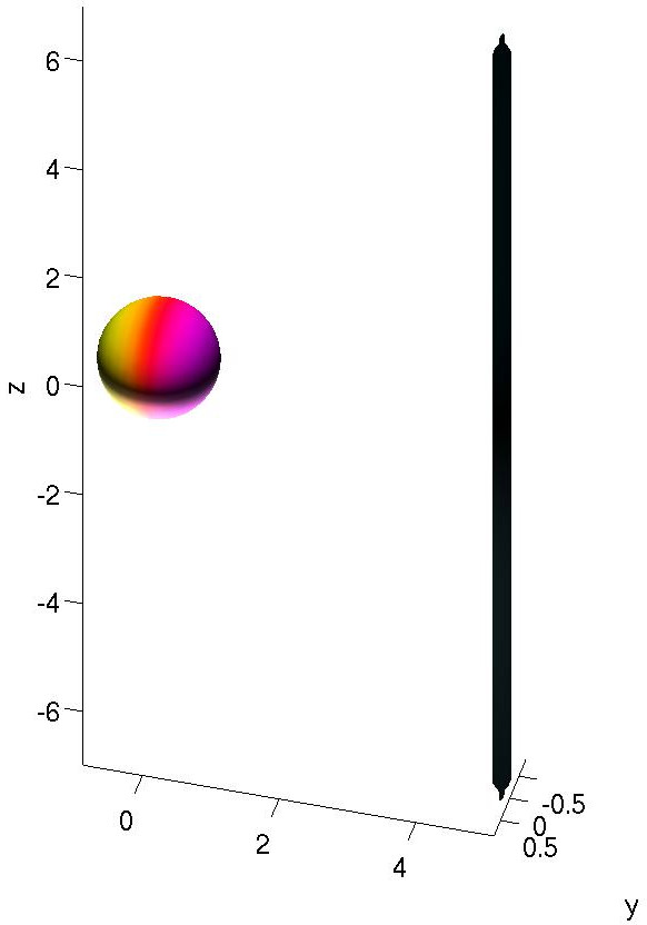
Figure 1: The absolute value of the energy density $|\mathcal{E}|$ of the configuration containing a 1-Skyrmion (the colored sphere) and a baby-Skyrmion string (the black vertical string).

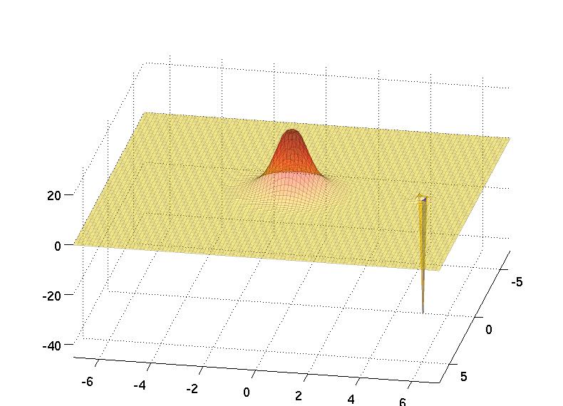
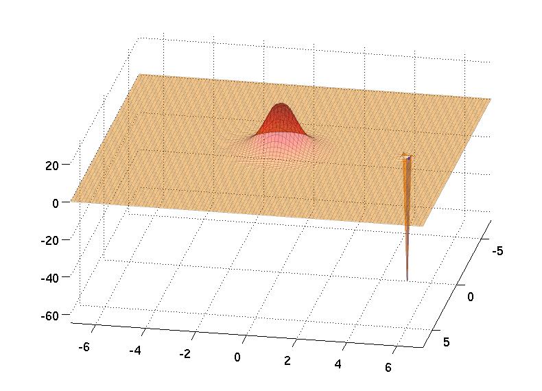
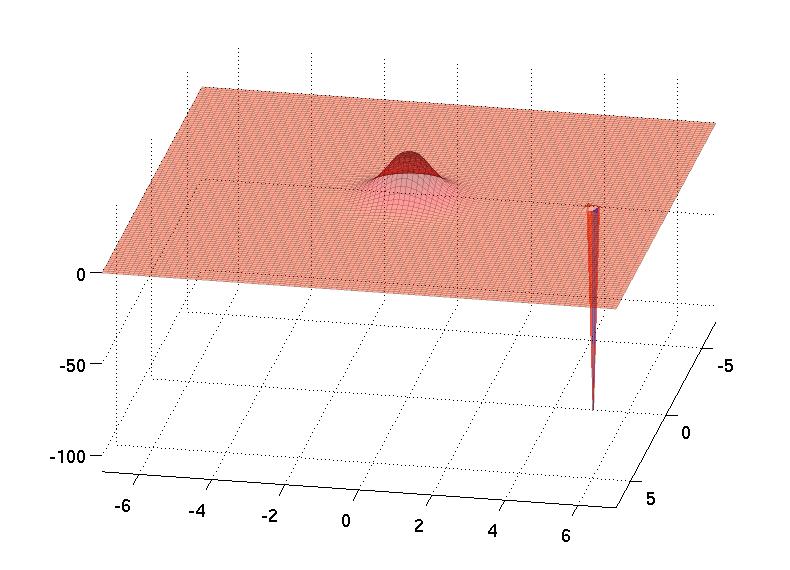
Figure 2: Cooling of the configuration shown in Fig. 1 at time $\tau=0$, $\tau=60$ and $\tau=120$, respectively. The figure shows the energy density in an $xy$-slice at fixed $z=0$. It is seen from the figure that the 1-Skyrmion is unchanged as cooling time increases, but the energy of the baby-Skyrmion string (to the right) is growing negative.

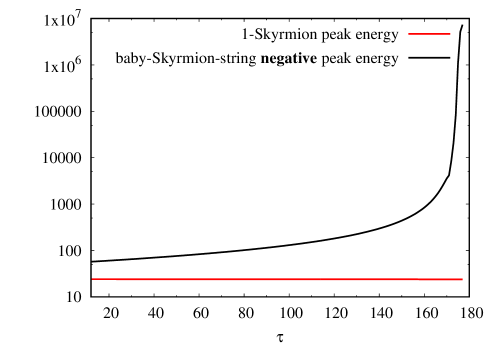
Figure 3: Peak energies: positive for the 1-Skyrmion and negative for the baby-Skyrmion string as functions of the cooling time $\tau$. It is seen from the figure that the 1-Skyrmion is unchanged, but the energy of the baby-Skyrmion string (to the right) is growing negative.

In Fig. 1 is shown the configuration at the initial time. The 1-Skyrmion is already the minimum of the energy functional and its fields have been found using the hedgehog Lagrangian (24) with $n=4$. The baby-Skyrmion string is not a topological object, but just a perturbation added to the configuration. In Fig. 2 is shown a series of three snapshots in cooling time $\tau=0,60,120$ of the configuration. The 1-Skyrmion is stable and remains a solution, but the baby-Skyrmion string is seen to grow more and more negative. Finally, we show the peak energies of the two objects in Fig. 3. The 1-Skyrmion has positive peak energy that remains stable, whereas the baby-Skyrmion string has a negative peak energy that grows rapidly more and more negative. This nicely illustrates the baby-Skyrmion string instability found in the Marleau construction.

Appendix B Difference from the Ostrogradsky instability

Let us compare the simplest possible term giving rise to four time derivatives in our theories with that of the Ostrogradsky-like theories,

$$\mathcal{L} =-\langle 1\rangle^{2}$$

$$=-(\partial_{\mu}\mathbf{n}\cdot\partial^{\mu}\mathbf{n})^{2}$$ (164)

which is just the kinetic term squared. Recall that the nonlinear sigma model constraint $\mathbf{n}\cdot\mathbf{n}=1$ implies

$$\frac{1}{2}\partial_{\mu}(\mathbf{n}\cdot\mathbf{n})=\mathbf{n}\cdot\partial_{\mu}\mathbf{n}=0.$$ (165)

Consider now integrating the Lagrangian (164) by parts as

$$\mathcal{L} =-(\partial_{\mu}\mathbf{n}\cdot\partial^{\mu}\mathbf{n})(\partial_{\nu}\mathbf{n}\cdot\partial^{\nu}\mathbf{n})$$

$$=-\partial_{\mu}\left[(\mathbf{n}\cdot\partial^{\mu}\mathbf{n})(\partial_{\nu}\mathbf{n}\cdot\partial^{\nu}\mathbf{n})\right]+(\mathbf{n}\cdot\partial_{\mu}\partial^{\mu}\mathbf{n})(\partial_{\nu}\mathbf{n}\cdot\partial^{\nu}\mathbf{n})+(\mathbf{n}\cdot\partial^{\mu}\mathbf{n})\partial_{\mu}(\partial_{\nu}\mathbf{n}\cdot\partial^{\nu}\mathbf{n})$$

$$=(\mathbf{n}\cdot\partial_{\mu}\partial^{\mu}\mathbf{n})(\partial_{\nu}\mathbf{n}\cdot\partial^{\nu}\mathbf{n})$$

$$=\partial_{\nu}\left[(\mathbf{n}\cdot\partial_{\mu}\partial^{\mu}\mathbf{n})(\mathbf{n}\cdot\partial^{\nu}\mathbf{n})\right]-\left[\partial_{\nu}(\mathbf{n}\cdot\partial_{\mu}\partial^{\mu}\mathbf{n})\right](\mathbf{n}\cdot\partial^{\nu}\mathbf{n})-(\mathbf{n}\cdot\partial_{\mu}\partial^{\mu}\mathbf{n})(\mathbf{n}\cdot\partial_{\nu}\partial^{\nu}\mathbf{n})$$

$$=-(\mathbf{n}\cdot\partial_{\mu}\partial^{\mu}\mathbf{n})(\mathbf{n}\cdot\partial_{\nu}\partial^{\nu}\mathbf{n}),$$ (166)

which obviously differs from the Ostrogradsky-like Lagrangian Woodard:2015zca

$$\mathcal{L} =-\partial_{\mu}\partial^{\mu}\mathbf{n}\cdot\partial_{\nu}\partial^{\nu}\mathbf{n}.$$ (167)

The reason why we do not have the Ostrogradsky instability, exactly, is because the propagator of Eq. (166) is not $p^{4}$; it remains $p^{2}$ and the term is still just a product of two kinetic terms.

Trying to formally manipulate the Ostrogradsky-like Lagrangian (167), we get

$$\mathcal{L} =-\partial_{\mu}\partial^{\mu}\mathbf{n}\cdot\partial_{\nu}\partial^{\nu}\mathbf{n}$$

$$=-(\partial_{\mu}\partial^{\mu}\mathbf{n}\cdot\partial_{\nu}\partial^{\nu}\mathbf{n})(\mathbf{n}\cdot\mathbf{n})$$

$$=-\partial_{\mu}\left[(\partial^{\mu}\mathbf{n}\cdot\partial_{\nu}\partial^{\nu}\mathbf{n})(\mathbf{n}\cdot\mathbf{n})\right]+(\partial^{\mu}\mathbf{n}\cdot\partial_{\mu}\partial_{\nu}\partial^{\nu}\mathbf{n})(\mathbf{n}\cdot\mathbf{n})+2(\partial^{\mu}\mathbf{n}\cdot\partial_{\nu}\partial^{\nu}\mathbf{n})(\mathbf{n}\cdot\partial_{\mu}\mathbf{n})$$

$$=-\partial_{\mu}\left[(\partial^{\mu}\mathbf{n}\cdot\partial_{\nu}\partial^{\nu}\mathbf{n})\right]+(\partial^{\mu}\mathbf{n}\cdot\partial_{\mu}\partial_{\nu}\partial^{\nu}\mathbf{n})+2\partial_{\nu}\left[(\partial^{\mu}\mathbf{n}\cdot\partial^{\nu}\mathbf{n})(\mathbf{n}\cdot\partial_{\mu}\mathbf{n})\right]$$

$$\phantom{=\ }-2(\partial^{\mu}\partial_{\nu}\mathbf{n}\cdot\partial^{\nu}\mathbf{n})(\mathbf{n}\cdot\partial_{\mu}\mathbf{n})-2(\partial^{\mu}\mathbf{n}\cdot\partial^{\nu}\mathbf{n})(\mathbf{n}\cdot\partial_{\mu}\partial_{\nu}\mathbf{n})-2(\partial^{\mu}\mathbf{n}\cdot\partial^{\nu}\mathbf{n})(\partial_{\nu}\mathbf{n}\cdot\partial_{\mu}\mathbf{n})$$

$$=-\partial_{\mu}\left[(\partial^{\mu}\mathbf{n}\cdot\partial_{\nu}\partial^{\nu}\mathbf{n})\right]+(\partial^{\mu}\mathbf{n}\cdot\partial_{\mu}\partial_{\nu}\partial^{\nu}\mathbf{n})+2\partial_{\nu}\left[(\partial^{\mu}\mathbf{n}\cdot\partial^{\nu}\mathbf{n})(\mathbf{n}\cdot\partial_{\mu}\mathbf{n})\right]$$

$$\phantom{=\ }-\partial^{\mu}\left[(\partial_{\nu}\mathbf{n}\cdot\partial^{\nu}\mathbf{n})(\mathbf{n}\cdot\partial_{\mu}\mathbf{n})\right]+(\partial_{\nu}\mathbf{n}\cdot\partial^{\nu}\mathbf{n})(\partial_{\mu}\mathbf{n}\cdot\partial^{\mu}\mathbf{n})+(\partial_{\nu}\mathbf{n}\cdot\partial^{\nu}\mathbf{n})(\mathbf{n}\cdot\partial_{\mu}\partial^{\mu}\mathbf{n})$$

$$\phantom{=\ }-2(\partial^{\mu}\mathbf{n}\cdot\partial^{\nu}\mathbf{n})(\mathbf{n}\cdot\partial_{\mu}\partial_{\nu}\mathbf{n})-2(\partial^{\mu}\mathbf{n}\cdot\partial^{\nu}\mathbf{n})(\partial_{\nu}\mathbf{n}\cdot\partial_{\mu}\mathbf{n})$$

$$=-\partial_{\mu}\left[(\partial^{\mu}\mathbf{n}\cdot\partial_{\nu}\partial^{\nu}\mathbf{n})\right]+(\partial^{\mu}\mathbf{n}\cdot\partial_{\mu}\partial_{\nu}\partial^{\nu}\mathbf{n})+(\partial_{\nu}\mathbf{n}\cdot\partial^{\nu}\mathbf{n})(\partial_{\mu}\mathbf{n}\cdot\partial^{\mu}\mathbf{n})$$

$$\phantom{=\ }+(\partial_{\nu}\mathbf{n}\cdot\partial^{\nu}\mathbf{n})(\mathbf{n}\cdot\partial_{\mu}\partial^{\mu}\mathbf{n})-2(\partial^{\mu}\mathbf{n}\cdot\partial^{\nu}\mathbf{n})(\mathbf{n}\cdot\partial_{\mu}\partial_{\nu}\mathbf{n})-2(\partial^{\mu}\mathbf{n}\cdot\partial^{\nu}\mathbf{n})(\partial_{\nu}\mathbf{n}\cdot\partial_{\mu}\mathbf{n}),$$ (168)

where in the last equation we have used Eq. (165). We can identify the $\langle 1\rangle^{2}$ and the $-2\langle 2\rangle$ terms in the last equation. However, deriving the constraint (165) once more, we get that

$$\partial_{\nu}\mathbf{n}\cdot\partial_{\mu}\mathbf{n}+\mathbf{n}\cdot\partial_{\mu}\partial_{\nu}\mathbf{n}=0,$$ (169)

where $\nu$ can also be equal to $\mu$ and summed over; it is a general statement derived from the nonlinear sigma model constraint. Using this relation, however, we can simplify Eq. (168) to

$$\mathcal{L} =-\partial_{\mu}\left[(\partial^{\mu}\mathbf{n}\cdot\partial_{\nu}\partial^{\nu}\mathbf{n})\right]+(\partial^{\mu}\mathbf{n}\cdot\partial_{\mu}\partial_{\nu}\partial^{\nu}\mathbf{n}),$$ (170)

which is simply the Ostrogradsky-like Lagrangian that we started with. Therefore, we can see that the Lagrangian (164) is not just the Ostrogradsky-like Lagrangian (167) up to a total derivative.

Nevertheless, this exercise should show that the Ostrogradsky system is intrinsically different from our Lagrangians and that we do not have $p^{4}$ in the propagator, but just a highly nonlinear theory.

References

- (1) T. H. R. Skyrme, “A Unified Field Theory of Mesons and Baryons,” Nucl. Phys. 31, 556 (1962). doi:10.1016/0029-5582(62)90775-7
- (2) T. H. R. Skyrme, “A Nonlinear field theory,” Proc. Roy. Soc. Lond. A 260, 127 (1961). doi:10.1098/rspa.1961.0018
- (3) E. Witten, “Global Aspects of Current Algebra,” Nucl. Phys. B 223, 422 (1983). doi:10.1016/0550-3213(83)90063-9
- (4) E. Witten, “Current Algebra, Baryons, and Quark Confinement,” Nucl. Phys. B 223, 433 (1983). doi:10.1016/0550-3213(83)90064-0
- (5) A. Zaks, “Derivation of the Skyrme-witten Lagrangian From QCD,” Nucl. Phys. B 260, 241 (1985). doi:10.1016/0550-3213(85)90321-9
- (6) T. Sakai and S. Sugimoto, “Low energy hadron physics in holographic QCD,” Prog. Theor. Phys. 113, 843 (2005) doi:10.1143/PTP.113.843 [hep-th/0412141].
- (7) G. H. Derrick, “Comments on nonlinear wave equations as models for elementary particles,” J. Math. Phys. 5, 1252 (1964). doi:10.1063/1.1704233
- (8) G. S. Adkins and C. R. Nappi, “Stabilization of Chiral Solitons via Vector Mesons,” Phys. Lett. 137B, 251 (1984). doi:10.1016/0370-2693(84)90239-9
- (9) A. Jackson, A. D. Jackson, A. S. Goldhaber, G. E. Brown and L. C. Castillejo, “A Modified Skyrmion,” Phys. Lett. 154B, 101 (1985). doi:10.1016/0370-2693(85)90566-0
- (10) L. Marleau, “The Skyrme Model and Higher Order Terms,” Phys. Lett. B 235, 141 (1990) Erratum: [Phys. Lett. B 244, 580 (1990)]. doi:10.1016/0370-2693(90)90110-R
- (11) L. Marleau, “Modifying the Skyrme model: Pion mass and higher derivatives,” Phys. Rev. D 43, 885 (1991). doi:10.1103/PhysRevD.43.885
- (12) L. Marleau, “All orders skyrmions,” Phys. Rev. D 45, 1776 (1992). doi:10.1103/PhysRevD.45.1776
- (13) L. Marleau and J. F. Rivard, “A generating function for all orders skyrmions,” Phys. Rev. D 63, 036007 (2001) doi:10.1103/PhysRevD.63.036007 [hep-ph/0011052].
- (14) C. Adam, J. Sanchez-Guillen and A. Wereszczynski, “A Skyrme-type proposal for baryonic matter,” Phys. Lett. B 691, 105 (2010) doi:10.1016/j.physletb.2010.06.025 [arXiv:1001.4544 [hep-th]].
- (15) C. Adam, J. Sanchez-Guillen and A. Wereszczynski, “A BPS Skyrme model and baryons at large ,” Phys. Rev. D 82, 085015 (2010) doi:10.1103/PhysRevD.82.085015 [arXiv:1007.1567 [hep-th]].
- (16) S. B. Gudnason and M. Nitta, “Baryonic sphere: a spherical domain wall carrying baryon number,” Phys. Rev. D 89, no. 2, 025012 (2014) doi:10.1103/PhysRevD.89.025012 [arXiv:1311.4454 [hep-th]].
- (17) S. B. Gudnason and M. Nitta, “Incarnations of Skyrmions,” Phys. Rev. D 90, no. 8, 085007 (2014) doi:10.1103/PhysRevD.90.085007 [arXiv:1407.7210 [hep-th]].
- (18) S. B. Gudnason and M. Nitta, “Baryonic torii: Toroidal baryons in a generalized Skyrme model,” Phys. Rev. D 91, no. 4, 045027 (2015) doi:10.1103/PhysRevD.91.045027 [arXiv:1410.8407 [hep-th]].
- (19) S. B. Gudnason and M. Nitta, “Fractional Skyrmions and their molecules,” Phys. Rev. D 91, no. 8, 085040 (2015) doi:10.1103/PhysRevD.91.085040 [arXiv:1502.06596 [hep-th]].
- (20) S. B. Gudnason and M. Nitta, “Skyrmions confined as beads on a vortex ring,” Phys. Rev. D 94, no. 2, 025008 (2016) doi:10.1103/PhysRevD.94.025008 [arXiv:1606.00336 [hep-th]].
- (21) E. A. Bergshoeff, R. I. Nepomechie and H. J. Schnitzer, “Supersymmetric Skyrmions in Four-dimensions,” Nucl. Phys. B 249, 93 (1985). doi:10.1016/0550-3213(85)90041-0
- (22) L. Freyhult, “The Supersymmetric extension of the Faddeev model,” Nucl. Phys. B 681, 65 (2004) doi:10.1016/j.nuclphysb.2004.01.012 [hep-th/0310261].
- (23) J. M. Queiruga, “Skyrme-like models and supersymmetry in 3+1 dimensions,” Phys. Rev. D 92, no. 10, 105012 (2015) doi:10.1103/PhysRevD.92.105012 [arXiv:1508.06692 [hep-th]].
- (24) S. B. Gudnason, M. Nitta and S. Sasaki, “A supersymmetric Skyrme model,” JHEP 1602, 074 (2016) doi:10.1007/JHEP02(2016)074 [arXiv:1512.07557 [hep-th]].
- (25) A. Nakamula, S. Sasaki and K. Takesue, “Atiyah-Manton Construction of Skyrmions in Eight Dimensions,” JHEP 1703, 076 (2017) doi:10.1007/JHEP03(2017)076 [arXiv:1612.06957 [hep-th]].
- (26) A. D. Jackson, C. Weiss and A. Wirzba, “Summing skyrmions,” Nucl. Phys. A 529, 741 (1991). doi:10.1016/0375-9474(91)90596-X
- (27) J.-P. Longpre and L. Marleau, “Simulated annealing for generalized Skyrme models,” Phys. Rev. D 71, 095006 (2005) doi:10.1103/PhysRevD.71.095006 [hep-ph/0502253].
- (28) J. P. Longpre and L. Marleau, “Multisoliton configurations in Skyrme-like models,” Can. J. Phys. 85, 679 (2007). doi:10.1139/p07-057
- (29) M. Ostrogradsky, “Mémoire sur les équations différentielles relatives au problème des isopérimètres,” Mem. Ac. Imp. Sci., St. Petersburg, Ser. VI T. 4, 385 (1850).
- (30) R. P. Woodard, “Ostrogradsky’s theorem on Hamiltonian instability,” Scholarpedia 10, no. 8, 32243 (2015) doi:10.4249/scholarpedia.32243 [arXiv:1506.02210 [hep-th]].
- (31) A. Pais and G. E. Uhlenbeck, “On Field theories with nonlocalized action,” Phys. Rev. 79, 145 (1950). doi:10.1103/PhysRev.79.145
- (32) N. S. Manton, “Geometry of Skyrmions,” Commun. Math. Phys. 111, 469 (1987). doi:10.1007/BF01238909
- (33) G. E. Andrews, “The theory of partitions,” Cambridge University Press, 1998.
- (34) J. F. Donoghue, “Quartic propagators, negative norms and the physical spectrum,” arXiv:1704.01533 [hep-th].
- (35) C. J. Halcrow, “Vibrational quantisation of the B = 7 Skyrmion,” Nucl. Phys. B 904, 106 (2016) doi:10.1016/j.nuclphysb.2016.01.011 [arXiv:1511.00682 [hep-th]].
- (36) C. Adam, M. Haberichter, T. Romanczukiewicz and A. Wereszczynski, “Radial vibrations of BPS skyrmions,” Phys. Rev. D 94, no. 9, 096013 (2016) doi:10.1103/PhysRevD.94.096013 [arXiv:1607.04286 [hep-th]].
- (37) C. J. Halcrow, C. King and N. S. Manton, “A dynamical -cluster model of 16O,” Phys. Rev. C 95, no. 3, 031303 (2017) doi:10.1103/PhysRevC.95.031303 [arXiv:1608.05048 [nucl-th]].
- (38) A. V. Smilga, “Ghost-free higher-derivative theory,” Phys. Lett. B 632, 433 (2006) doi:10.1016/j.physletb.2005.10.014 [hep-th/0503213].
- (39) A. V. Smilga, “Comments on the dynamics of the Pais-Uhlenbeck oscillator,” SIGMA 5, 017 (2009) doi:10.3842/Sigma.2009.017 [arXiv:0808.0139 [quant-ph]].
- (40) M. Pavšič, “Stable Self-Interacting Pais-Uhlenbeck Oscillator,” Mod. Phys. Lett. A 28, 1350165 (2013) doi:10.1142/S0217732313501654 [arXiv:1302.5257 [gr-qc]].
- (41) M. Pavšič, “Pais–Uhlenbeck oscillator and negative energies,” Int. J. Geom. Meth. Mod. Phys. 13, no. 09, 1630015 (2016) doi:10.1142/S0219887816300154 [arXiv:1607.06589 [gr-qc]].
- (42) M. Eto, M. Nitta, K. Ohashi and D. Tong, “Skyrmions from instantons inside domain walls,” Phys. Rev. Lett. 95, 252003 (2005) doi:10.1103/PhysRevLett.95.252003 [hep-th/0508130].
- (43) M. Eto, T. Fujimori, M. Nitta, K. Ohashi and N. Sakai, “Higher Derivative Corrections to Non-Abelian Vortex Effective Theory,” Prog. Theor. Phys. 128, 67 (2012) doi:10.1143/PTP.128.67 [arXiv:1204.0773 [hep-th]].
- (44) S. B. Gudnason, M. Nitta and N. Sawado, “Gravitating BPS Skyrmions,” JHEP 1512, 013 (2015) doi:10.1007/JHEP12(2015)013 [arXiv:1510.08735 [hep-th]].
- (45) S. B. Gudnason, M. Nitta and N. Sawado, “Black hole Skyrmion in a generalized Skyrme model,” JHEP 1609, 055 (2016) doi:10.1007/JHEP09(2016)055 [arXiv:1605.07954 [hep-th]].
- (46) C. Adam, O. Kichakova, Y. Shnir and A. Wereszczynski, “Hairy black holes in the general Skyrme model,” Phys. Rev. D 94, no. 2, 024060 (2016) doi:10.1103/PhysRevD.94.024060 [arXiv:1605.07625 [hep-th]].
- (47) I. Perapechka and Y. Shnir, “Generalized Skyrmions and hairy black holes in asymptotically AdS4 spacetime,” Phys. Rev. D 95, no. 2, 025024 (2017) doi:10.1103/PhysRevD.95.025024 [arXiv:1612.01914 [hep-th]].
- (48) J. M. Speight, “A pure Skyrme instanton,” Phys. Lett. B 659, 429 (2008) doi:10.1016/j.physletb.2007.10.040 [hep-th/0703198 [HEP-TH]].
- (49) S. B. Gudnason, M. Nitta and S. Sasaki, “Topological solitons in the supersymmetric Skyrme model,” JHEP 1701, 014 (2017) doi:10.1007/JHEP01(2017)014 [arXiv:1608.03526 [hep-th]].
- (50) C. Adam, J. M. Queiruga, J. Sanchez-Guillen and A. Wereszczynski, “N=1 supersymmetric extension of the baby Skyrme model,” Phys. Rev. D 84, 025008 (2011) doi:10.1103/PhysRevD.84.025008 [arXiv:1105.1168 [hep-th]].
- (51) C. Adam, J. M. Queiruga, J. Sanchez-Guillen and A. Wereszczynski, “Extended Supersymmetry and BPS solutions in baby Skyrme models,” JHEP 1305, 108 (2013) doi:10.1007/JHEP05(2013)108 [arXiv:1304.0774 [hep-th]].
- (52) M. Nitta and S. Sasaki, “BPS States in Supersymmetric Chiral Models with Higher Derivative Terms,” Phys. Rev. D 90, no. 10, 105001 (2014) doi:10.1103/PhysRevD.90.105001 [arXiv:1406.7647 [hep-th]].
- (53) S. Bolognesi and W. Zakrzewski, “Baby Skyrme Model, Near-BPS Approximations and Supersymmetric Extensions,” Phys. Rev. D 91, no. 4, 045034 (2015) doi:10.1103/PhysRevD.91.045034 [arXiv:1407.3140 [hep-th]].
- (54) M. Nitta and S. Sasaki, “Higher Derivative Corrections to Manifestly Supersymmetric Nonlinear Realizations,” Phys. Rev. D 90, no. 10, 105002 (2014) doi:10.1103/PhysRevD.90.105002 [arXiv:1408.4210 [hep-th]].
- (55) M. Nitta and S. Sasaki, “Classifying BPS States in Supersymmetric Gauge Theories Coupled to Higher Derivative Chiral Models,” Phys. Rev. D 91, 125025 (2015) doi:10.1103/PhysRevD.91.125025 [arXiv:1504.08123 [hep-th]].