Schnyder woods, SLE₁₆, and Liouville quantum gravity

Abstract.

In 1990, Schnyder used a 3-spanning-tree decomposition of a simple triangulation, now known as the Schnyder wood, to give a fundamental grid-embedding algorithm for planar maps. In the framework of mating of trees, a uniformly sampled Schnyder-wood-decorated triangulation can produce a triple of random walks. We show that these three walks converge in the scaling limit to three Brownian motions produced in the mating-of-trees framework by Liouville quantum gravity (LQG) with parameter $1$, decorated with a triple of SLE₁₆’s curves. These three SLE₁₆’s curves are coupled such that the angle difference between them is $2\pi/3$ in imaginary geometry. Our convergence result provides a description of the continuum limit of Schnyder’s embedding algorithm via LQG and SLE.

1. Introduction

A planar map is an embedding of a connected planar graph in the plane, considered modulo orientation-preserving homeomorphism. A planar map is said to be simple if it does not have any edges from a vertex to itself or multiple edges between the same pair of vertices. We say that a planar map is a triangulation if every face is bounded by three edges. A spanning tree of a graph $G$ is a connected, cycle-free subgraph of $G$ including all vertices of $G$. In this paper we will study wooded triangulations, which are simple triangulations equipped with a certain 3-spanning-tree decomposition known as a Schnyder wood.

The Schnyder wood, also referred to as a graph realizer in the literature, was introduced by Walter Schnyder [57] to prove a characterization of graph planarity. He later used Schnyder woods to describe an algorithm for embedding an order-$n$ planar graph in such a way that its edges are straight lines and its vertices lie on an $(n-2)\times(n-2)$ grid [58]. Schnyder’s celebrated construction has continued to play an important role in graph theory and enumerative combinatorics [6, 20, 53].

In the present article, we are primarily interested in the $n\to\infty$ behavior of wooded triangulations and their Schnyder embeddings. We discover an encoding of the wooded triangulation via a triple of random walks, where the coordinates of vertices under the Schnyder embedding are natural observables of the random walks. As we will explain in Sections 1.2–1.4, each of these three random walks fits into the mating-of-trees framework developed in [62, 15]. By simply applying the invariance principle for a single random walk, we may obtain a scaling limit result (Theorem 1.5) for wooded triangulation in the peanosphere sense. However, to understand the large-scale behavior of the Schnyder embedding, we need to study the interaction between the three spanning trees. This relies on another crucial observation we make in this paper: the coupling of the three trees is analogous to the coupling of a certain triple of continuum trees formed by imaginary geometry flow lines. The technical bulk of this paper (Section 5) is to develop this insight and ultimately establish a scaling limit result (Theorem 1.6) for the image of a typical wooded triangulation under the Schnyder embedding.

1.1. Wooded triangulations

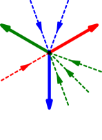
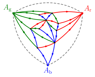
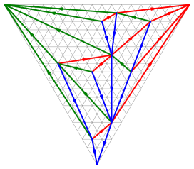
Figure 1. (a) Schnyder’s coloring rule: all incoming edges of a given color appear between the outgoing edges of the other two colors. We draw the incoming arrows as dashed to indicate that the number of incoming edges of a given color may be zero. (b) The edges of a planar triangulation can be decomposed into three spanning trees satisfying Schnyder’s coloring rule, and (c) Schnyder’s algorithm uses this triple of trees to output a grid embedding of the triangulation.

Consider a simple plane triangulation $M$ with unbounded face $\triangle A_{\mathrm{b}}A_{\mathrm{g}}A_{\mathrm{r}}$ where the outer vertices $A_{\mathrm{b}}$, $A_{\mathrm{g}}$, and $A_{\mathrm{r}}$—which we think of as blue, green, and red—are arranged in clockwise order. Here simple means with no multiple edges and self-loops. We denote by $\overline{A_{\mathrm{b}}A_{\mathrm{g}}}$ the edge connecting $A_{\mathrm{b}}$ and $A_{\mathrm{g}}$, and similarly for $\overline{A_{\mathrm{g}}A_{\mathrm{r}}}$ and $\overline{A_{\mathrm{r}}A_{\mathrm{b}}}$. Vertices, edges, and faces of $M$ other than $A_{\mathrm{b}},A_{\mathrm{g}},A_{\mathrm{r}},\overline{A_{\mathrm{b}}A_{\mathrm{g}}},\overline{A_{\mathrm{g}}A_{\mathrm{r}}},\overline{A_{\mathrm{r}}A_{\mathrm{b}}}$ and $\triangle A_{\mathrm{b}}A_{\mathrm{g}}A_{\mathrm{r}}$ are called inner vertices, edges, and faces respectively. We define the size of $M$ to be the number of interior vertices. Euler’s formula implies that a simple plane triangulation of size $n$ has $n+3$ vertices, $3n+3$ edges, and $2n+2$ faces.

An orientation on $M$ is a choice of direction for every inner edge of $M$, and a 3-orientation on $M$ is an orientation for which every inner vertex has out-degree $3$. Each simple triangulation admits at least one 3-orientation [58]. A coloring of the inner edges of a 3-orientation with the colors blue, green, and red is said to satisfy Schnyder’s rule (see Figure 1(a)) if (i) the three edges exiting each interior vertex are colored in the clockwise cyclic order blue-green-red, and (ii) each blue edge $e$ which enters an interior vertex $v$ does so between $v$’s red and green outgoing edges, and similarly for the other incoming edges. In other words, incoming red edges at a given vertex (if there are any) must appear between green and blue outgoing edges, and incoming green edges appear between blue and red outgoing edges. As demonstrated in As shown in [58], given 3-orientation $\mathcal{O}$ on a simple triangulation $M$, there is a unique way of coloring the inner edges such that Schnyder’s rule is satisfied. We describe this coloring as an algorithm which we call COLOR.

1. Color $A_{\mathrm{b}},A_{\mathrm{g}},A_{\mathrm{r}}$ blue, green, and red.

2. For each inner edge $e$, construct a directed path $\mathcal{P}=[e_{1},e_{2},\cdots e_{\ell}]$ inductively as follows. Set $e_{1}=e$. For $k\geq 1$: if the head of $e_{k}$ is an outer vertex, set $\ell=k$ and stop. Otherwise, let $e_{k+1}$ be the second outgoing edge encountered when clockwise (or equivalently, counterclockwise) rotating $e_{k}$ about its head. (Here the head vertex and tail vertex of an orientated edge are such that the orientation goes from the tail to the head.) This procedure always yields a finite path without cycle. To see this, note that if $\mathcal{P}$ has a cycle $\gamma$ of length $m$, then the planar map $M^{\prime}$ consisting of the faces of $M$ enclosed by $\gamma$ (together with a single unbounded face) would have $m+v$ vertices where $v$ is the number of vertices surrounded by $\gamma$. Moreover, $M^{\prime}$ has $E=2m+3v$ edges since each vertex on $\gamma$ contributes two outgoing edges, and each vertex not on $\gamma$ contribute three. By Euler’s formula $M$ would have $F=2v+m-2$ faces. Since $M^{\prime}$ is a triangulation except one face, we have $m+3(F-1)=2E$, a contradiction.

3. Assign to $e$ the color of the outer vertex at which $\mathcal{P}$ terminates.

We now summarize a few properties of COLOR that are essentially from [58]; also see the notes [45]:

1. Edges on a path $\mathcal{P}$ have the same color.

2. Given an inner vertex $v$ with outgoing edges $e_{1},e_{2},e_{3}$, the three paths starting from $e_{1},e_{2},e_{3}$ are all simple paths, namely without cycles.

3. Given an inner vertex $v$ with outgoing edges $e_{1},e_{2},e_{3}$, the three paths starting from $e_{1},e_{2},e_{3}$ do not intersect except at $v$. This may be proved similarly to #1.

4. Since the three paths emanating from $v$ are simple and non-intersecting, the three paths must terminate at distinct outer vertices. Therefore, their colors are distinct and appear in the same cyclic order as the exterior vertices.

5. As a consequence of #1 and #4, Schnyder’s coloring rule is satisfied. Indeed, if $v$ is an inner vertex and $e$ is an oriented edge in between the green and red outgoing edges from $v$, then the blue outgoing edge from $v$ must be the next edge on the path starting from $e$. Therefore $e$ itself is blue.

6. The set of all blue edges forms a spanning tree of $M\backslash\{A_{\mathrm{g}},A_{\mathrm{r}}\}$, and similarly for red and green. These three trees form a partition of the set of $M$’s interior edges.

Definition 1.1.

Given a simple plane triangulation $M$ equipped with a 3-orientation, we call a coloring of the interior edges satisfying Schnyder’s rule a Schnyder wood on $M$. We denote by $\mathcal{S}_{n}$ the set of pairs $(M,\mathcal{O})$ where $M$ is a triangulation of size $n$ equipped with a 3-orientation and $\mathcal{O}$ is a Schnyder wood on $M$. We will refer to elements of $\bigcup_{n\geq 1}\mathcal{S}_{n}$ as Schnyder-wood-decorated triangulations, or wooded triangulations for short.

The COLOR algorithm exhibits a natural bijection between Schnyder woods on $M$ and 3-orientations on $M$. Accordingly, we will treat Schnyder woods and 3-orientations as interchangeable. For a wooded triangulation $S$, denote by $T_{c}(S)$ the tree of color $c$ on $S$, for $c\in\{\mathrm{b,r,g}\}$. We call the unique blue oriented path from a vertex $v$ the blue flow line from $v$, and similarly for red and green.

1.2. SLE, Liouville quantum gravity, and random planar maps

The Schramm Loewner evolution with a parameter $\kappa>0$ (abbreviated to $\operatorname{SLE}_{\kappa}$) is a well-known family of random planar curves discovered by Schramm [59]. These curves enjoy conformal symmetries and a natural Markov property which establish SLE as a canonical family of non-self-crossing planar curves. For a large class of 2D statistical physics models such as percolation and Ising model, it is proved or conjectured that their scaling limit at criticality are described by $\operatorname{SLE}_{\kappa}$ curve with various $\kappa$; see e.g.  [63, 42, 41, 60, 64, 9].

Liouville quantum gravity with parameter $\gamma\in(0,2)$ (abbreviated to $\gamma$-LQG) is a family of random planar geometries formally corresponding to $e^{\gamma h}\,dx\otimes dy$, where $h$ is a 2D random generalized function called the Gaussian free field (GFF) and $\gamma$ indexes the roughness of the geometry. Rooted in theoretical physics, LQG is closely related to conformal field theory and string theory [55]. It is also an important tool for studying planar fractals through the Knizhnik-Polyakov-Zamolodchikov relation (see [16] and references therein). Most importantly for our purposes, LQG describes the scaling limit of decorated random planar maps. Let’s discuss this perspective in the context of a classical example called the uniform-spanning-tree-decorated random planar map.

For each $\gamma\in(0,2)$, there exists a canonical random surface of spherical topology whose geometry is given by $\gamma$-LQG. The surface is called the unit-area $\gamma$-LQG sphere. Its area measure is of the form $\mu_{\mathfrak{h}}=e^{\sqrt{2}\mathfrak{h}}\,dx\,dy$ where $\mathfrak{h}$ is a particular variant of Gaussian free field. Due to the roughness of $\mathfrak{h}$, the rigorous construction of $\mu_{\mathfrak{h}}$ requires a regularization and normalization procedure called the Gaussian multiplicative chaos (GMC). We refer to the book [4] for the background on LQG, GFF and GMC. More details for $\mathfrak{h}$ and $\mu_{\mathfrak{h}}$ in will be provided in Section 4.1. We now explain how the unit-area $\sqrt{2}$-LQG sphere is related to the scaling limit of the uniform-spanning-tree-decorated random planar map.

Let $\mathcal{M}_{n}$ be the set of pairs $(M,T)$ such that $M$ is an $n$-edge planar map and $T$ is a spanning tree on $M$. Let $(M_{n},T_{n})$ be a uniform sample from $\mathcal{M}_{n}$ and conformally embed $M_{n}$ in $\mathbb{C}$, for example via circle packing or Riemann uniformization ( see e.g. [24, Section 2]). Define an atomic measure on $\mathbb{C}$ by associating a unit mass with each vertex in this embedding of $M_{n}$. It is conjectured that this measure, suitably renormalized, converges as $n\to\infty$ to a unit-mass random area measure $\mu_{\mathfrak{h}}$ on $\mathbb{C}$, which is the aforementioned area measure for the unit-area $\sqrt{2}$-LQG sphere. Let $\eta_{n}$ be the Peano curve which snakes between $T_{n}$ and its dual. It is conjectured that $\eta_{n}$ converges to an $\operatorname{SLE}_{8}$ that is independent of $\mu_{\mathfrak{h}}$. (Convergence to $\operatorname{SLE}_{8}$ of the uniform spanning tree on the square lattice is proved in [42]).

One can replace the spanning tree in the above discussion with other structures, such as percolation, Ising model, or random cluster models. Under certain conformal embeddings, random planar maps decorated with models are believed to converge to unit area $\gamma$-LQG sphere s decorated with $\operatorname{SLE}_{\gamma^{2}}$ and $\operatorname{SLE}_{16/\gamma^{2}}$ curves, for some $\gamma\in(0,2)$. As metric spaces, they are believed to converge to a random metric space that formally has $e^{\gamma\mathfrak{h}}dx\otimes dy$ as its metric tensor. The rigorous construction of the random metric was recently achieved by [12, 28] using a regularization and normalization procedure. Both of the two types of convergence remain unproved except for the percolation-decorated random planar map, in which case $M_{n}$ is uniformly distributed. LeGall [44] and Miermont [46] independently proved that the metric scaling limit is a random metric space called the Brownian map. Miller and Sheffield [49, 51, 52] rigorously established an identification of the Brownian map and $\sqrt{8/3}$-LQG. Recently in [34] Holden and the second named author of this paper proved that uniform triangulation under a certain discrete conformal embedding converges to $\sqrt{8/3}$-LQG. Gwynne, Miller and Sheffield [31, 30, 29] showed that certain random planar map models obtained from coarse-graining the continuum LQG converge to the LQG under another discrete conformal embedding called the Tutte embedding. Here we remark that the Schnyder embedding considered in this paper is not a discrete conformal embedding.

Duplantier, Miller, and Sheffield [15, 62] developed a powerful approach to LQG which is particularly suited to build connections between random planar map and LQG. The starting point is a bijection due to Mullin [54] and Bernardi [5] between the set $\mathcal{M}_{n}$ and the set of lattice walks on $\mathbb{Z}^{2}_{\geq 0}$ with $2n$ steps and starting and ending at the origin. Here a lattice walk means a possible trajectory of a random walk on $\mathbb{Z}^{2}$. The walk corresponding to $(M,T)$ is obtained by keeping track of the graph distances in $T$ and its dual $\tilde{T}$ from the tip of the exploration curve $\eta_{n}$ to two specified roots. This bijection is an example of a family of bijections that are now known as mating-of-trees bijections, because the exploration curve can be thought of as stitching the two trees $T$ and $\tilde{T}$ together.

This mating-of-trees story can be carried out in the continuum as well, with LQG playing the role of the planar map and $\operatorname{SLE}$ the role of the Peano curve. Suppose $(\mu_{\mathfrak{h}},\eta^{\prime})$ is the conjectured scaling limit of a certain decorated random planar map under conformal embedding for some $\gamma\in(0,2)$, as described above. Namely, $\mu_{\mathfrak{h}}$ is area measure of the unit-area $\gamma$-LQG sphere, and $\eta^{\prime}$ is a variant of SLE_κ with $\kappa=16/\gamma^{2}$ which is independent of $\mathfrak{h}$. As explained in [15], the curve $\eta^{\prime}$ can be parametrized so that $\eta^{\prime}$ is a continuous space-filling curve from $[0,1]$ to $\mathbb{C}\cup\{\infty\}$, $\eta^{\prime}(0)=\eta^{\prime}(1)=\infty$ and $\mu_{\mathfrak{h}}(\eta^{\prime}([s,t]))=t-s$ for $0<s<t<1$. By [61, 15], one can define lengths $\mathscr{L}_{t}$ and $\mathscr{R}_{t}$ for the left and right boundaries of $\eta^{\prime}{[0,t]}$ with respect to $\mu_{\mathfrak{h}}$. The following mating-of-trees theorem is proved in [15, 50, 22].

Theorem 1.2.

In the above setting, the law of $(\mathscr{Z}_{t})_{t\in[0,1]}=(\mathscr{L}_{t},\mathscr{R}_{t})_{t\in[0,1]}$ can be sampled as follows. First sample a two-dimensional Brownian motion $\mathscr{Z}=(\mathscr{L},\mathscr{R})$ with

(1.1) $$\operatorname{Var}[\mathscr{L}_{t}]=\operatorname{Var}[\mathscr{R}_{t}]=t\quad\textrm{and}\quad\operatorname{Cov}[\mathscr{L}_{t},\mathscr{R}_{t}]=-\cos\left(\tfrac{\pi\gamma^{2}}{4}\right)t.$$

Then condition $\mathscr{Z}|_{[0,1]}$ on the event that both $\mathscr{L}$ and $\mathscr{R}$ stay positive in $(0,1)$ and $\mathscr{L}_{1}=\mathscr{R}_{1}=0$. Moreover, $\mathscr{Z}$ determines $(\mu_{\mathfrak{h}},\eta^{\prime})$ a.s.

The singular conditioning referred to in this theorem statement can be made rigorous by a limiting procedure [50, Section 3]. In light of the Mullin-Bernardi bijection and Theorem 1.2, the convergence of the 2D lattice walks to the 2D Brownian motion (namely the invariance principle) can be viewed as a convergence of the spanning-tree-decorated random planar map $(M_{n},T_{n})$ to $\sqrt{2}$-LQG decorated with an independent $\operatorname{SLE}_{8}$. We say that this convergence is in the peanosphere sense. The same type of convergence has been established for several models; see [62, 27, 32, 33, 37, 23, 26, 35]. In many cases, the topology of convergence can be further improved by using special properties of the model of interest [27, 33, 23]. In particular, results in [8] are crucial to the aforementioned convergence in [34] under conformal embedding. See [24] for a survey on the mating of trees theory and its application to random planar maps. We will provide more background on SLE, GFF, and LQG in Section 4. But we emphasize that the mating of trees framework allows us to work mostly on the Brownian motion side. Thus most of the paper does not require this background.

1.3. A Schnyder wood mating-of-trees encoding

We consider a uniform sample $(M_{n},\mathcal{O}_{n})$ from $\mathcal{S}_{n}$, which we call a uniform wooded triangulation of size $n$. We view $(M_{n},\mathcal{O}_{n})$ as a decorated random planar map. Under the marginal law of $M_{n}$, the probability of each triangulation is proportional to the number of Schnyder woods it admits. Conditioned on $M_{n}$, the law of $S_{n}$ is uniform on the set of Schnyder woods on $M_{n}$. We are interested in the scaling limit of $(M_{n},\mathcal{O}_{n})$ as $n\to\infty$.

Our starting point is a bijection similar to the Mullin-Bernardi bijection for spanning-tree-decorated planar maps in Section 1.2. Suppose $S\in\mathcal{S}_{n}$. We define a path $\mathcal{P}_{S}$ (see Figure 2(b)) which starts in the outer face, enters an inner face through $\overline{A_{\mathrm{r}}A_{\mathrm{g}}}$, crosses all edges incident to $A_{\mathrm{g}}$, enters the outer face through $\overline{A_{\mathrm{g}}A_{\mathrm{b}}}$, enters an inner face through $\overline{A_{\mathrm{g}}A_{\mathrm{b}}}$, explores $T_{\mathrm{b}}(S)$ clockwise, enters the outer face through $\overline{A_{\mathrm{b}}A_{\mathrm{r}}}$, enters an inner face through $\overline{A_{\mathrm{b}}A_{\mathrm{r}}}$, crosses the edges incident to $A_{\mathrm{r}}$, enters the outer face through $\overline{A_{\mathrm{r}}A_{\mathrm{g}}}$, and returns at the starting point. The path $\mathcal{P}_{S}$ crosses $\overline{A_{\mathrm{r}}A_{\mathrm{g}}}$, $\overline{A_{\mathrm{g}}A_{\mathrm{b}}}$ and $\overline{A_{\mathrm{b}}A_{\mathrm{r}}}$ and each red and green edge twice and traverses each blue edge twice. Namely, we can view the path $\mathcal{P}_{S}$ as an ordering of the edge set of $S$ where each inner edge is visited twice.

Define $\varphi(S)=Z^{\mathrm{b}}$ to be a walk on $\mathbb{Z}^{2}$ as follows. The walk starts at $(0,0)$. When $\mathcal{P}_{S}$ traverses a blue edge for the second time, $Z^{\mathrm{b}}$ takes a $(1,-1)$-step. When $\mathcal{P}_{S}$ crosses a red edge for the second time, $Z^{\mathrm{b}}$ takes a $(-1,0)$-step. When $\mathcal{P}_{S}$ crosses a green edge for the second time, $Z^{\mathrm{b}}$ takes a $(0,1)$-step. See Figure 9 for an example of a pair $(S,\varphi(S))$.

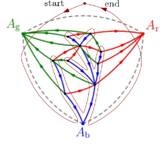
Figure 2. (a) a triangulation equipped with a Schnyder wood, and (b) the path $\mathcal{P}_{S}$, which traces out the blue tree clockwise.

Definition 1.3.

Define $\mathcal{W}_{n}$ to be the set of walks on $\mathbb{Z}^{2}$ satisfying the following conditions.

1. The walk starts and ends at $(0,0)$ and stays in the closed first quadrant.

2. The walk has $3n$ steps, of three types: $(0,1)$, $(-1,0)$ and $(1,-1)$.

3. No $(1,-1)$-step is immediately preceded by a $(-1,0)$-step.

Theorem 1.4.

We have $\varphi(S)\in\mathcal{W}_{n}$ for all $S\in\mathcal{S}_{n}$, and $\varphi:\mathcal{S}_{n}\to\mathcal{W}_{n}$ is a bijection.

By symmetry, we may also define $Z^{\mathrm{r}}$ and $Z^{\mathrm{g}}$ similarly to $Z^{\mathrm{b}}$, based on clockwise explorations of $T_{\mathrm{r}}$ and $T_{\mathrm{g}}$, respectively. Theorem 1.4 implies that the $Z^{\mathrm{r}}$ and $Z^{\mathrm{g}}$ encodings are also bijective. We will prove Theorem 1.4 in Section 2.1.

1.4. SLE₁₆-decorated 1-LQG as the scaling limit

We now describe a conjectural scaling limit of the uniform-wooded triangulation in terms of LQG surface decorated by SLE curves. Our Theorem 1.5 is a verification of this conjecture in the mating of trees framework. Since there are three spanning trees, we need three space-filling SLE curves that are coupled together. Imaginary geometry is a framework that produces such couplings, which is developed in [47, 48]. Fix $\kappa>4$, in this framework, there is a notion of angle between two different space-filling SLE_κ. We will provide more details of imaginary geometry and the coupling between different SLE curves in Section 4.1. On the other hand, as mentioned before, we mainly focus on the Brownian motion side of the mating-of-trees story, hence details of this coupling from the SLE side is not necessary to understand our result.

To state our conjecture and theorem, we consider three space-filling $\operatorname{SLE}_{16}$ curves coupled in imaginary geometry, where the angle difference between each other is $2\pi/3$. We denote the three space-filling curves by $(\eta^{\mathrm{b}},\eta^{\mathrm{r}},\eta^{g})$ and let $\mathfrak{h}$ be the field corresponding to a unit-area $1$-LQG sphere which is independent of $(\eta^{\mathrm{b}},\eta^{\mathrm{r}},\eta^{\mathrm{g}})$. The marginal law $(\mathfrak{h},\eta^{\bullet})$ for $\bullet=\mathrm{b},\mathrm{r},\mathrm{g}$ is the same as $(\mathfrak{h},\eta^{\prime})$ in Theorem 1.2. with $\gamma=1$. The precise description of the joint law of $(\eta^{\mathrm{b}},\eta^{\mathrm{r}},\eta^{g})$ will be given in Section 4.1. Let $S_{n}$ be a uniform wooded triangulation of size $n$. We conjecture that, under a conformal embedding and a suitable normalization, the volume measure of $S_{n}$ converges to $\mu_{\mathfrak{h}}$, and that the clockwise exploration curves of the three trees in $S_{n}$ jointly converge to $\eta^{\mathrm{b}},\eta^{\mathrm{r}},$ and $\eta^{\mathrm{g}}$. Our following theorem verifies the mating-of-trees variant of this conjecture.

Theorem 1.5.

Suppose $(Z^{\mathrm{b}},Z^{\mathrm{r}},Z^{\mathrm{g}})$ is the triple of random walks encoding the three trees in a uniformly sampled wooded triangulation of size $n$. For $\mathrm{c}\in\{\mathrm{b},\mathrm{r},\mathrm{g}\}$, let $\mathscr{Z}^{c}$ be the Brownian excursion associated with $(\eta^{c},\mu_{\mathfrak{h}})$ as in Theorem 1.2. Namely $(\mathscr{Z}^{c},\mu_{\mathfrak{h}},\eta^{c})$ has the same law as $(\mathscr{Z},\mu_{\mathfrak{h}},\eta^{\prime})$ in Theorem 5.1. Write $Z^{\mathrm{c}}=(L^{\mathrm{c}},R^{\mathrm{c}})$. Then

(1.2) $$\left(\tfrac{1}{\sqrt{4n}}L^{\mathrm{c}}_{\lfloor 3nt\rfloor},\tfrac{1}{\sqrt{2n}}R^{\mathrm{c}}_{\lfloor 3nt\rfloor}\right)_{t\in[0,1]}\stackrel{{\scriptstyle\text{in law}}}{{\longrightarrow}}(\mathscr{Z}^{\mathrm{c}})_{t\in[0,1]}\quad\textrm{for}\;\;\mathrm{c}\in\{\mathrm{b},\mathrm{r},\mathrm{g}\}.$$

Furthermore, the three convergence statements in (1.2) hold jointly.

Figure 3. The random walks $Z^{\mathrm{b}},Z^{\mathrm{r}},$ and $Z^{\mathrm{g}}$ under the scaling in Theorem 1.5.

This theorem is a natural extension of the idea that $M_{n}$ and one of its trees converge in the peanosphere sense. The one-tree version boils down to a classical statement about random walk convergence. The three-tree version requires a more detailed analysis, because the triple $(\mathscr{Z}^{\mathrm{b}},\mathscr{Z}^{\mathrm{r}},\mathscr{Z}^{\mathrm{\mathrm{g}}})$ is more complicated than a six-dimensional Brownian motion.

1.5. Schnyder’s embedding and its continuum limit

It is well-known that every planar graph admits a straight-line planar embedding [18, 66]. A longstanding problem in computational geometry was to find a straight-line drawing algorithm such that (i) every vertex has integer coordinates, (ii) every edge is drawn as a straight line, and (iii) the embedded graph occupies a region with $O(n)$ height and $O(n)$ width. This was achieved independently by de Fraysseix, Pach, and Pollack [21] and by Schnyder [58] via different methods. Schnyder’s algorithm is an elegant application of the Schnyder wood:

1. Given an arbitrary planar graph $G$, there exists a simple maximal planar supergraph $M$ of $G$ (in other words, a simple triangulation $M$ of which $G$ is a subgraph—note that $M$ is not unique). Such a triangulation $M$ can be identified in linear (that is, $O(n)$) time and with $O(n)$ faces, so the problem is reduced to the case of simple triangulations.

2. The triangulation $M$ admits at least one Schnyder wood structure, and one can be found in linear time. So we may assume $M$ is equipped with a Schnyder wood.

3. Each vertex $v$ in $M$, the blue, red, green flow lines from $v$ partition $M$ into three regions. Let $x(v)$, $y(v)$, and $z(v)$ be the number of faces in these three regions, as shown in Figure 4(a), and define $s(v)=(x(v),y(v),z(v))$. It is possible, in linear time, to compute the values of $s(v)$ for all vertices $v$ [58].

4. Since the total number of inner faces is some constant $F$, the range of the map $s(v)=(x(v),y(v),z(v))$ is contained in the intersection of $\mathbb{Z}^{3}$, the plane $x+y+z=F$, and the closed first octant. This intersection is an equilateral-triangle-shaped portion of the triangular lattice $T$ (see Figure 4(b)). It is proved combinatorially in [58] that if we map every edge $(u,v)$ in $M$ to the line segment between $s(u)$ and $s(v)$, then we obtain a proper embedding (that is, no such line segments intersect except at common endpoints). Note that height and width of $T$ are $O(n)$.

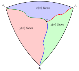
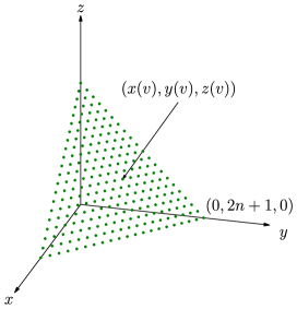
Figure 4. Schnyder’s embedding: we send each vertex $v$ in a simple plane triangulation to the triple of integers describing the number of faces in each region into which the flow lines from $v$ partition the planar map.

Schnyder’s method and de Fraysseix, Pach, and Pollack’s method provided the foundational ideas upon which subsequent straight-line grid embedding schemes have been built. For more discussion, we refer the reader to [11, 66].

In Schnyder’s algorithm, the coordinates of a vertex $v$ are determined by how flow lines from $v$ partition the faces of $M_{n}$. Since these ingredients have continuum analogues, Theorem 1.5 suggests that Liouville quantum gravity coupled with imaginary geometry can be used to describe the large-scale random behavior of Schnyder’s embedding. Consider the coupling of $(\mu_{\mathfrak{h}},\eta^{b},\eta^{r},\eta^{g})$ as in Theorem 1.5. Given $v\in\mathbb{C}$, run three flow lines from $u$, which are the right boundaries of $\eta^{\mathrm{b}},\eta^{\mathrm{r}},$ and $\eta^{\mathrm{g}}$ at the respective times when they first hit $u$. Map $u$ to the point in the plane $x+y+z=1$ whose coordinates $x(v)$, $y(v)$, and $z(v)$ are given by the $\mu_{\mathfrak{h}}$-measure of the three regions into which these flow lines partition $\mathbb{C}$. This map is the continuum analogue of the discrete map depicted in Figure 4.

Theorem 1.6.

Consider a uniform wooded triangulation of size $n$, and let $v^{n}_{1},\cdots,v_{k}^{n}$ be an i.i.d. list of uniformly chosen elements of the vertex set. Then the list of embedded locations of these vertices, namely $\{(2n)^{-1}s(v_{i}^{n})\}_{1\leq i\leq k}$, converges in law as $n\to\infty$.

The limiting law is that of $\{x(v_{i}),y(v_{i}),z(v_{i})\}_{1\leq i\leq k}$, where $v_{1},\cdots,v_{k}$ are $k$ points uniformly and independently sampled from an instance of $\mu_{\mathfrak{h}}$.

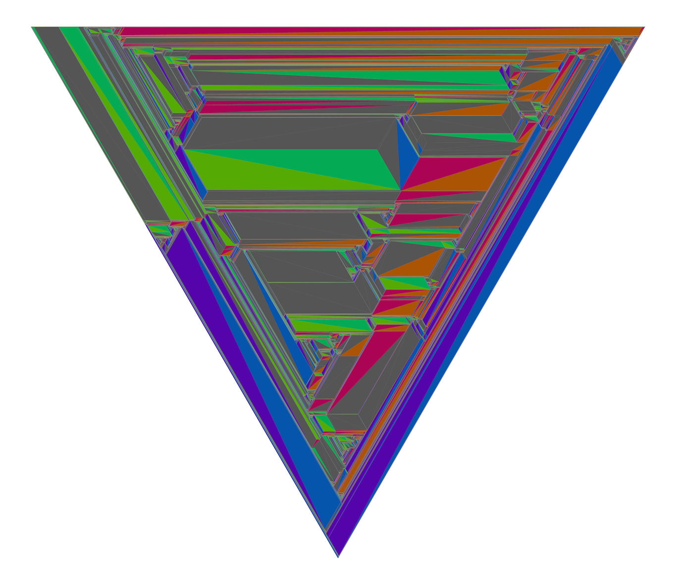
Figure 5. A uniformly sampled 1,000,000-vertex Schnyder-wood-decorated triangulation, Schnyder-embedded in an equilateral triangle. Each face is colored with the average (in RGB color space) of the colors of its three bounding edges.

We will prove Theorem 1.6 as a corollary to our proof of Theorem 1.5.

Remark 1.7.

In the discrete setting, there are exactly three flow lines from every vertex. In the continuum, this flow line uniqueness holds almost surely for any fixed point, but not for all points simultaneously. That is, there almost surely exist multiple flow lines of the same angle starting from the same point. This singular behavior is manifested in some noteworthy features of the image of a large uniform wooded triangulation under the Schnyder embedding (Figure 5). For example, there are macroscopic triangles occupying the full area of the overall triangle. These macroscopic triangles come in pairs which form parallelograms, whose sides are parallel to the sides of the overall triangle. In Theorem 1.6, we focus on typical points. A more thorough discussion of the continuum limit of the Schnyder embedding and its relation to imaginary geometry singular points will appear in [65].

1.6. Relation to other models and works

Bipolar orientations

A bipolar orientation on a planar map is an acyclic orientation with a unique source and sink. A mating-of-trees bijection for bipolar-oriented maps was found in [37], and the authors used it to prove that bipolar-oriented planar maps converge to $\operatorname{SLE}_{12}$ decorated $\sqrt{4/3}$-LQG, in the peanosphere sense. A bipolar orientation also induces a bipolar orientation on the dual map. In [37], the authors conjectured that the bipolar-decorated map and its dual jointly converge to $\sqrt{4/3}$-LQG decorated with two $\operatorname{SLE}_{12}$ curves coupled in the same imaginary geometry. In [23], this conjecture was proved in the triangulation case. The convergence is of the same type as in our Theorem 1.5. The angle between the two $\operatorname{SLE}_{12}$ curves is $\pi/2$. This was the first time that a pair of imaginary-geometry-coupled Peano curves was proved to be the scaling limit of a natural discrete model. The present article provides the first example for a triple of Peano curves. Our work will make use of some results on the coupling of multiple imaginary geometry trees from [23]. We will review these results in Section 4.2.

Given $S\in\mathcal{S}_{n}$, let $M^{\prime}=T_{\mathrm{b}}(S)\cup T_{\mathrm{g}}(S)\cup\overline{A_{g}A_{b}}$, and reverse the orientation of each blue edge. It is proved in [19, Proposition 7.1] that (i) this operation gives a bipolar oriented map on $n+2$ vertices with the property that the right side of every bounded face is of length two, and (ii) this procedure gives a bijection between $\mathcal{S}_{n}$ and the set of bipolar oriented maps with that property. Applying the mating-of-trees bijection in [37], it can be proved that the resulting walk coincides with the walk $\mathcal{Z}^{n}$ in Lemma 3.1. Furthermore, both blue and green flow lines in $S$ can be thought of as flow lines in the bipolar orientation on the dual map of $M^{\prime}$ in the sense of [37]. Therefore, Theorem 1.5 can be formulated as a result for bipolar orientations. However, the bipolar orientation perspective clouds some combinatorial elements that are useful for the probabilistic analysis. Therefore, rather than making use of this bijection, we will carry out a self-contained development of the requisite combinatorics directly in the Schnyder woods setting. See [25] for an application of this bipolar orientation encoding, where the authors showed that the metric exponent for uniform wooded triangulation is the same as the corresponding exponent for LQG with $\gamma=1$.

Non-intersecting Dyck paths

In [6], the authors give a bijection between the set of wooded triangulations and the set of pairs of non-crossing Dyck paths. This bijection implies that the number of wooded triangulations of size $n$ is equal to

(1.3) $$C_{n+2}C_{n}-C_{n+1}^{2}=\frac{6(2n)!(2n+2)!}{n!(n+1)!(n+2)!(n+3)!}$$

where $C_{n}$ is the $n$-th Catalan number [6, Section 3]. Our bijection is similar to the one in [6] in that they are both based on a contour exploration of the blue tree. In fact, their bijection is related to ours via a shear transformation that maps the first quadrant to $\{(x,y)\in\mathbb{R}^{2}\,:\,x\geq y\geq 0\}$. Thus Theorem 1.5 implies that the three pairs of non-intersecting Dyck paths in [6]—coming from clockwise exploring the three trees— converge jointly to a shear transform of $(\mathscr{Z}^{\mathrm{b}},\mathscr{Z}^{\mathrm{r}},\mathscr{Z}^{\mathrm{g}})$ in Theorem 1.5.

The non-crossing Dyck paths are closely related to the lattice structure of the set of Schnyder woods on a triangulation, while our bijection is designed to naturally encode geometric information about the wooded triangulation.

Twenty-vertex model

Note that a Schnyder wood on a regular triangular lattice has the property that each vertex has in-degree and out-degree 3. In other words, Schnyder woods are equivalent to Eulerian orientations in this case. Similarly, bipolar orientations on the square lattice have in-degree and out-degree 2 at each vertex. In the terminology of the statistical physics literature, these are the twenty-vertex and six-vertex models, respectively (note that $20=\binom{6}{3}$ and $6=\binom{4}{2}$). The twenty-vertex model was first studied by Baxter [2], following the suggestion of Lieb. Baxter [2] showed that the residual entropy of the twenty-vertex model is $\tfrac{3\sqrt{3}}{2}$, generalizing Lieb’s famous result for the six-vertex model.

Since the twenty-vertex model is a special case of the Schnyder wood, we may define flow lines from each vertex using the COLOR algorithm. Furthermore, we may consider the dual orientation on the dual lattice—this orientation sums to zero around each hexagonal face and can therefore be integrated to give a height function associated with the model. It is an easy exercise to check that the winding change of a flow line in the twenty-vertex model can be measured by the height difference along the flow line. This is analogous to the Temperley bijection for the dimer model, where the dimer height function measures the winding of the branches of the spanning tree generated by the dimer model. A similar flow-line height function relation for the six-vertex model has been found by [38]. In light of the correspondence between the dimer model and imaginary geometry with $\kappa=2$, we conjecture that the twenty-vertex model is similarly related to imaginary geometry with $\kappa=1$. To our knowledge, this perspective on the twenty-vertex model is new. We will not elaborate on it in this paper, but we plan to do some numerical study in a future work. See [38] for results on the numerical study of the six-vertex model in this direction.

Bernardi and Fusy decomposition.

Bernardi and Fusy [7] provides a Schnyder decomposition for $d$-angulations of girth $d$, generalizing the bipolar orientation ($d=4$) and Schnyder woods $(d=3)$. It is interesting to understand the relation between LQG and their model for $d\geq 5$, in particular, the corresponding LQG parameter $\gamma$.

1.7. Outline

In Section 2 we show that our relation between wooded triangulations and lattice walks is a bijection, and we demonstrate how this bijection operates locally. We use this construction to define an infinite-volume version of the uniform wooded triangulation, for ease of analysis. In Section 3 we prove convergence of the planar map and one tree, and we address some technically important relationships between various lattice walk variants associated with the same wooded triangulation. In Section 4 we review the requisite LQG and imaginary geometry material, and we present a general-purpose excursion decomposition of a two-dimensional Brownian motion that plays a key role in connecting $Z^{\mathrm{b}}$, $Z^{\mathrm{r}}$ and $Z^{\mathrm{g}}$. Finally, in Sections 5.1–5.3 we prove the infinite volume version of Theorem 1.5, namely Theorem 5.1. In Section 5.4, we transfer Theorem 5.1 to the finite volume setting and conclude the proofs of Theorems 1.5 and 1.6.

2. Schnyder woods and 2D random walks

We will prove Theorem 1.4 in Section 2.1 and record some geometric observations in Section 2.2. In Section 2.3, we construct the infinite volume limit of the uniform wooded triangulation.

2.1. From a wooded triangulation to a lattice walk

We first recall some basics on rooted plane trees. For more background, see [43]. A rooted plane tree is a planar map with one face and a specified directed edge called the root edge. The head of the root edge is called the root of the tree. We will use the term tree as an abbreviation for rooted plane tree throughout.

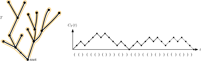
Figure 6. A rooted plane tree whose root edge is indicated with an arrow. The contour function $C_{T}$ (shown here linearly interpolated) tracks the graph distance to the root for a clockwise traversal of the tree. The contour function is a Dyck path, and if we associate to each $+1$ step an open parenthesis and with each $-1$ step a closed parenthesis, then we see that Dyck paths of length $2n$ are in bijection with parenthesis matchings of length $2n$.

Let $n$ be a positive integer, and suppose $T$ is a tree with $n+1$ vertices and $n$ edges. Without loss of generality, we draw $T$ on the plane such that (i) its root is below all other vertices and (ii) the root edge is to the left hand side of other edges attached to the root. Consider a clockwise exploration of $T$ starting from the left side of the root edge (see Figure 6), and define a function $C_{T}$ from $\{0,1,\cdots,2{\color[rgb]{0,0,0}n}\}$ to $\mathbb{Z}$ such that $C_{T}(0)=0$ and for $0\leq t\leq 2{\color[rgb]{0,0,0}n}-1$, $C_{T}(t+1)-C_{T}(t)=+1$ if the $(t+1)$st step of the exploration traverses its edge in the away-from-the-root direction and $-1$ otherwise. We call $C_{T}$ the contour function associated with $T$.

The contour function is an example of a Dyck path of length $2{\color[rgb]{0,0,0}n}$: a nonnegative walk from $\{0,1,\ldots,2{\color[rgb]{0,0,0}n}\}$ to $\mathbb{Z}$ with steps in $\{-1,+1\}$ which starts and ends at 0. We can linearly interpolate the graph of $C_{T}$ and glue the result along maximal horizontal segments lying under the graph to recover $T$ from $C_{T}$. Thus $T\mapsto C_{T}$ is a bijection from the set of rooted plane trees with $n$ edges to the set of Dyck paths of length $2{\color[rgb]{0,0,0}n}$.

A parenthesis matching is a word in two symbols ( and ) that reduces to the empty word under the relation $\texttt{()}=\emptyset$. The gluing action mapping $C_{T}$ to $T$ is equivalent to parenthesis matching the steps of $C_{T}$, with upward steps as open parentheses and down steps as close parentheses (see Figure 6). Thus the set of Dyck paths of length $2n$ is also in natural bijection with the set of parenthesis matchings of length $2n$.

Suppose $S=(M,\mathcal{O})$ is a wooded triangulation, and denote by $T_{\mathrm{b}}(S)$ its blue tree. Among the edges of $T_{\mathrm{b}}(S)$, we let the one immediately clockwise from $\overline{A_{\mathrm{g}}A_{\mathrm{b}}}$ around $A_{\mathrm{b}}$ be the root edge of $T_{\mathrm{b}}(S)$, and similarly for the red and green trees. Let the heads of these root edges be the outer vertices. So their orientations are consistent with the corresponding 3-orientation and $T_{\mathrm{b}}(S)$, $T_{\mathrm{r}}(S)$, and $T_{\mathrm{g}}(S)$ are rooted plane trees.

Given a lattice walk $Z$ whose increments are in $\{(1,-1),(-1,0),(0,1)\}$, we define the associated word $w=w_{1}w_{2}\cdots w_{3n}$ in the letters $\{\mathrm{b,r,g}\}$ by mapping the sequence of increments of $Z$ to its corresponding sequence of colors: for $1\leq k\leq 3n$ we define $w_{k}$ to be $\mathrm{b}$ if $Z_{k}-Z_{k-1}=(1,-1)$, to be r if $Z_{k}-Z_{k-1}=(-1,0)$, and to be g if $Z_{k}-Z_{k-1}=(0,1)$ (see Figure 9). We will often elide the distinction between a walk and its associated word, so we can say $w\in\mathcal{W}_{n}$ if $w$ is the word associated to $Z$ and $Z\in\mathcal{W}_{n}$. Also, we will refer to the two components of an ordered pair as its abscissa and ordinate, respectively.

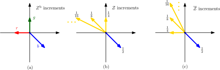
Figure 7. The set of increments of the three types of lattice walk we consider: (a) $Z^{\mathrm{b}}$: $(1,-1)$, $(0,1)$, and $(-1,0)$, (b) $\mathcal{Z}$ (see Lemma 3.1 and 3.2): $\{(1,-1)\}\cup(-\mathbb{Z}_{\geq 0}\times\{1\})$, with probability measure indicated by the labels, and (c) $\overline{\mathcal{Z}}$ (see Definition 5.5): $\{(1,-1)\}\cup(\{-1\}\times\mathbb{Z}_{\geq 0})$.

Given a word $w$, let $w_{\mathrm{g}\mathrm{b}}$ be the sub-word obtained by dropping all r symbols from $w$ and $w_{\mathrm{b}\mathrm{r}}$ be the sub-word obtained by dropping all g symbols from $w$. Then $w\in\mathcal{W}_{n}$ implies that both $w_{\mathrm{g}\mathrm{b}}$ and $w_{\mathrm{b}\mathrm{r}}$ are parenthesis matchings:

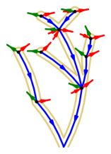
Figure 8. We cut each red and green edge into incoming and outgoing arrows at each vertex and discard the green incoming arrows. Then associating the second traversing of each blue edge with the outgoing red arrow incident to its tail, we see that $w_{\mathrm{b}\mathrm{r}}$ encodes the matching of red incoming and outgoing arrows along the contour of the blue tree. Similarly, associating each outgoing green arrow with the first traversing of the outgoing blue edge from the same vertex, we see that $w_{\mathrm{b}\mathrm{r}}$ describes the contour function of the blue tree.

Proposition 2.1.

For $S\in\mathcal{S}_{n}$, we have $w\colonequals{\color[rgb]{0,0,0}\varphi}(S)\in\mathcal{W}_{n}$. Moreover, $w_{\mathrm{g}\mathrm{b}}$ is the parenthesis matching corresponding to the contour function of $T_{\mathrm{b}}$, and $w_{\mathrm{br}}$ is the parenthesis matching describing $\mathcal{P}_{S}$’s crossings of the red edges (to wit: each first crossing corresponds to an open parenthesis, and each second crossing to a close parenthesis).

Proof.

From Schnyder’s rule and the COLOR algorithm, $\mathcal{P}_{S}$ crosses each green (resp. red) edge $e$ twice, and the tail (resp. head) of $e$ is on the right of $\mathcal{P}_{S}$ at the second crossing.

Obviously $S$ has $n$ edges in each color, so $\varphi(S)$ has $n$ steps in each type and must end at the origin. For each blue edge, the Schnyder’s rule for its tail implies that the $(1,-1)$-step corresponding to this blue edge must be preceded by the $(0,1)$-step corresponding to the outgoing green edge at the tail of this blue edge. So the $\varphi(S)$ cannot go below the upper half plane. For each red edge, if its tail is $v$, then $\mathcal{P}_{S}$ traverses the outgoing blue edge at $v$ for the second time before $\mathcal{P}_{S}$ crosses this red edge for the second time. So the $(-1,0)$-step corresponding to this red edge must be after the $(1,-1)$-step corresponding to the outgoing blue edge at $v$, therefore $\varphi(S)$ never goes to the left half plane. In summary, $\varphi(S)\in\mathcal{W}_{n}$.

We remove the outer edges and cut all of the green and red edges into outgoing and incoming arrows (a.k.a darts). Then every g (resp. r) symbol in $w$ corresponds to a green outgoing (resp. red incoming) arrow. Finally, we remove incoming green arrows (see Figure 8).

The outgoing and incoming red arrows in this arrow-decorated tree form a valid parenthesis matching, by planarity of $S$. By Schnyder’s rule, each b in $w$ corresponds to the blue edge whose second traversal immediately follows $\mathcal{P}_{S}$’s crossing of some outgoing red arrow. Using this identification between outgoing red arrows and b’s in $w$, we see that the sequence of b’s and r’s in $w_{\mathrm{b}\mathrm{r}}$ admits the same parenthesis matching as the sequence of outgoing and incoming red arrows. So $w_{\mathrm{br}}$ is the parenthesis matching describing $\mathcal{P}_{S}$’s crossings of the red edges. Similarly, identifying the outgoing green arrow and outgoing blue edge from each vertex $v$, Schnyder’s rule implies that only incoming red arrows may appear between $\mathcal{P}_{S}$’s first traversal of $v$’s outgoing blue edge and its crossing of $v$’s outgoing green arrow. Thus $w_{\mathrm{g}\mathrm{b}}$ admits the same parenthesis matching as the contour function of the blue tree. ∎

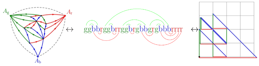
Figure 9. With each wooded triangulation we associate a word and a lattice walk. The values of the lattice walk are perturbed slightly to make it easier to visually follow the path. The green (resp. red) curves above (resp. below) the word denotes the $\mathrm{g}\mathrm{b}$ (resp. $\mathrm{b}\mathrm{r}$) matches.

Recall that a combinatorial map is a graph together with a (clockwise) cyclic order of the edges incident to each vertex. From this data, we may define combinatorial faces and information about how these faces are connected along edges and at vertices. Gluing together polygons according to these rules, we get a surface $X$ together with an embedding of the combinatorial map in $X$. This embedding is unique up to deformation of $X$ [39].

For any word $w$ in the symbols b, r, and g, we say that $(w_{j},w_{k})$ is a gb match if $w_{j}=\mathrm{g}$, $w_{k}=\mathrm{b}$, and sub-word obtained by dropping the r’s from $w_{j+1}\cdots w_{k-1}$ reduces to the empty word under the relation $\mathrm{g}\mathrm{b}=\emptyset$. We also say $w_{k}$ (resp. $w_{j}$) is the gb match of $w_{j}$ (resp. $w_{k}$). We define the term br match similarly. By the constructions of the gb match and the br match, if a letter in $w$ has a gb (resp. br) match, then the gb (resp. br) match must be unique.

The following definition provides a recipe to recover a wooded triangulation from its word.

Definition 2.2.

Given $w\in\mathcal{W}_{n}$, we define a graph $\psi(w)$ with colored oriented edges as follows. The vertex set is the union of the set of $\mathrm{b}$’s in $w$ and the symbols $\{A_{\mathrm{b}},A_{\mathrm{r}},A_{\mathrm{g}}\}$. A vertex $v$ is called an outer vertex if $v\in\{A_{\mathrm{b}},A_{\mathrm{r}},A_{\mathrm{g}}\}$ and an inner vertex otherwise. We define $\overline{A_{\mathrm{b}}A_{\mathrm{r}}},\overline{A_{\mathrm{r}}A_{\mathrm{g}}},$ and $\overline{A_{\mathrm{g}}A_{\mathrm{b}}}$ to be the three outer edges of $\psi(w)$. For each $1\leq i\leq 3n$, we define an inner edge associated with $w_{i}$ as follows (see Figure 10):

1. For $w_{i}=\mathrm{b}$, if there exists $(j,k)$ such that $j<i<k$ and $(w_{j},w_{k})$ is a $\mathrm{g}\mathrm{b}$ match, find the least such $k$ and construct a blue edge from $w_{i}$ to $w_{k}$. Otherwise construct a blue edge from $w_{i}$ to $A_{\mathrm{b}}$.

2. For $w_{i}=\mathrm{r}$, find $w_{i}$’s $\mathrm{b}\mathrm{r}$ match $(w_{i^{\prime}},w_{i})$. If there exists $j>i$ with $w_{j}=\mathrm{g}$, find the smallest such $j$ and identify $w_{j}$’s $\mathrm{g}\mathrm{b}$ match $(w_{j},w_{k})$. Construct a red edge from $w_{i^{\prime}}$ to $w_{k}$. Otherwise construct a red edge from $w_{i^{\prime}}$ to $A_{\mathrm{r}}$.

3. For $w_{i}=\mathrm{g}$, find $w_{i}$’s $\mathrm{g}\mathrm{b}$ match $(w_{i},w_{i^{\prime}})$. If there exists $(j,k)$ such that $j<i<k$ and $(w_{j},w_{k})$ is a $\mathrm{b}\mathrm{r}$ match, find the greatest such $j$ and construct a green edge from $w_{i^{\prime}}$ to $w_{j}$. Otherwise, construct a green edge from $w_{i^{\prime}}$ to $A_{\mathrm{g}}$.

Here we identify symbols in $w$ with inner edges of $\psi(w)$ and identify b symbols with inner vertices of $\psi(w)$ (the tail of a blue edge identified with a b symbol is the vertex corresponding to that b symbol).

By the edge assigning rule, each inner vertex has exactly one outgoing edge of each color. We now upgrade $\psi(w)$ to a combinatorial map by defining a clockwise cyclic order around each vertex. For an inner vertex, the clockwise cycling order is the following and obeys Schnyder’s rule: the unique blue outgoing edge, the incoming red edges, the unique outgoing green edge, the incoming blue edges, the unique outgoing red edge, incoming green edges. We also have to specify the order for incoming edges of each color: the incoming blue edges are in order of the appearance of their corresponding $\mathrm{b}$-symbol in $w$; same rules apply for incoming red edges; the incoming green edges are in the reverse order of appearance of their corresponding $\mathrm{g}$-symbol in $w$.

For the edges attached to $A_{\mathrm{b}}$, we define the clockwise cyclic order by $\overline{A_{\mathrm{b}}A_{\mathrm{g}}}$, followed by incoming blue edges in order of the appearance in $w$, followed by $\overline{A_{\mathrm{b}}A_{\mathrm{r}}}$. For the edges attached to $A_{\mathrm{r}}$, we define the clockwise cyclic order by $\overline{A_{\mathrm{r}}A_{\mathrm{b}}}$, followed by incoming red edges in order of the appearance in $w$, followed by $\overline{A_{\mathrm{r}}A_{\mathrm{g}}}$. For the edges attached to $A_{\mathrm{g}}$, we define the clockwise cyclic order by $\overline{A_{\mathrm{g}}A_{\mathrm{r}}}$, followed by incoming green edges in the reverse order of the appearance in $w$, followed by $\overline{A_{\mathrm{g}}A_{\mathrm{b}}}$.

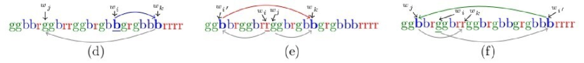
Figure 10. The relevant portions of the path $\mathcal{P}(S)$ for the construction of (a) blue edges, (b) red edges, and (c) green edges. And an illustration of how to construct inner edges from its word in Definition 2.2: (d) blue edges, (e) red edges, and (f) green edges

We will use the following two lemmas to conclude the proof of Theorem 1.4. Given a word $w\in\mathcal{W}_{n}$, define $\mathcal{M}_{\mathrm{b}\mathrm{r}}(w)$ to be the submap of $\psi(w)$ whose edge set consists of all of the blue edges, all of the red edges, and $\overline{A_{\mathrm{b}}A_{\mathrm{r}}}$, and whose vertex set consists of all the vertices of $\psi(w)$ except $A_{\mathrm{g}}$.

Lemma 2.3.

$\mathcal{M}_{\mathrm{b}\mathrm{r}}(w)$ is a planar map, for all $w\in\mathcal{W}_{n}$.

Proof.

Let $\mathcal{M}_{\mathrm{b}}$ be the subgraph of $\psi(w)$ consisting of all its blue edges. Recall the definition of blue edges in Definition 2.2. We can embed $\mathcal{M}_{\mathrm{b}}$ on the plane so that $w_{\mathrm{g}\mathrm{b}}$ is its Dyck word and $A_{b}$ is the head of its root. Moreover $\overline{T}_{\mathrm{b}}:=T_{\mathrm{b}}\cup\{\overline{A_{\mathrm{b}}A_{\mathrm{r}}}\}$ is a spanning tree of $\mathcal{M}_{\mathrm{b}\mathrm{r}}$. We further embed $\overline{A_{\mathrm{b}}A_{\mathrm{r}}}$ so that it is the last edge in the clockwise exploration of $\overline{T}_{\mathrm{b}}$. Now we cut each red edge of $\mathcal{M}_{\mathrm{b}\mathrm{r}}$ into an incoming and outgoing arrow so that $\mathcal{M}_{\mathrm{b}\mathrm{r}}$ is transformed to $\overline{T}_{\mathrm{b}}$ with $2n$ total red arrows attached at its vertices. Now we can embed the red arrows in the plane uniquely so that the edge ordering around each vertex is consistent with the ordering rule in Definition 2.2.

For each inner vertex $v$ we find the symbol $w_{i}=\mathrm{b}$ corresponding to $v$. Let $w_{j}=\mathrm{g}$ and $w_{k}=\mathrm{r}$ be the gb match and br match of $w_{i}$ respectively. Then by Definition 2.2, the edges corresponding to $w_{i},w_{j},w_{k}$ are the unique blue, green, red outgoing edges from $v$. We identify the red outgoing arrow from $w_{k}$ with the b symbol $w_{i}$. Let $\ell=\max\{m<j:w_{m}\neq\mathrm{r}\}$. Then there exists an incoming red arrow at $v$ if and only if $w_{j-1}=\mathrm{r}$ and the $\mathrm{r}$ symbols corresponding to these incoming arrows, appearing in clockwise order, are $w_{\ell+1},\cdots,w_{j-1}$. Let $\ell_{0}=\max\{m:w_{m}\neq\mathrm{r}\}$. Then the $\mathrm{r}$ symbols corresponding to the incoming red arrows at $A_{\mathrm{r}}$, appearing in clockwise order, are $w_{\ell_{0}+1},\ldots,w_{3n}$. Therefore if we clockwise-explore $\overline{T}_{\mathrm{b}}$, the $2n$ red arrows encountered appear in the same order as in $w_{\mathrm{b}\mathrm{r}}$, where each b (resp., r) symbol corresponds to an outgoing (resp., incoming) arrow. Since $w_{\mathrm{b}\mathrm{r}}$ is a parenthesis matching, we may link red arrows in a planar way to recover $\mathcal{M}_{\mathrm{b}\mathrm{r}}$. ∎

Since $\mathcal{M}_{\mathrm{b}\mathrm{r}}(w)$ is planar, we may embed it in the plane so that the face right of $\overline{A_{\mathrm{b}}A_{\mathrm{r}}}$ is the unbounded face. We now describe the face structure of $\mathcal{M}_{\mathrm{b}\mathrm{r}}$. Let $Z^{\mathrm{b}}=(L^{\mathrm{b}},R^{\mathrm{b}})$ be the walk corresponding to $w$. For each $w_{i}=\mathrm{b}$, let $v$ be its corresponding inner vertex and $w_{j}=\mathrm{r}$ be the br match of $w_{i}$. Then the blue and red outgoing edges from $v$ are $w_{i}$ and $w_{j}$. Let

(2.1) $$\mathcal{G}_{i}=\left\{k>i:w_{k}=\mathrm{g}\;\textrm{ and }\;L^{\mathrm{b}}_{k}=L^{\mathrm{b}}_{i}=\min_{i\leq j\leq k}L^{\mathrm{b}}_{j}\right\}.$$

By Definition 2.2, there exist incoming green edges attached to $v$ if and only if $\mathcal{G}_{i}\neq\emptyset$. In this case, write elements in $\mathcal{G}_{i}$ as $k_{1}<\cdots<k_{m}$. Then $i<k_{1}<\cdots<k_{m}<j$ and the green edges attached to $v$ in counterclockwise order between $w_{i}$ and $w_{j}$ are $w_{k_{1}}\cdots,w_{k_{m}}$. Let $v_{0}$ (resp., $v_{m+1}$) be the head of $w_{i}$ (resp., $w_{j}$). For $1\leq\ell\leq m$, let $v_{\ell}$ be the tail of $w_{k_{\ell}}$. Let $\mathcal{F}(e)$ be the face of $\mathcal{M}_{\mathrm{b}\mathrm{r}}$ on the left of $e$ where $e$ is the blue edge corresponding to $w_{i}$. The following lemma describes the structure of $\mathcal{F}(e)$.

Lemma 2.4.

The vertices on $\mathcal{F}(e)$ are $v,v_{0},\cdots,v_{m+1}$ in counterclockwise order.

Furthermore, $\mathcal{F}$ is a bijection between blue edges and inner faces of $\mathcal{M}_{\mathrm{b}\mathrm{r}}$.

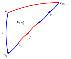
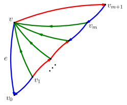
Figure 11. (a) Each face of $\mathcal{M}_{\mathrm{b}\mathrm{r}}$, traversed counterclockwise, consists of a blue forward-oriented edge $e$, followed by a sequence of reverse blue or forward red edges, followed by a reverse red edge back to $e$’s tail. (b) The green edges triangulate each face of $\mathcal{M}_{\mathrm{b}\mathrm{r}}$.

Proof.

First note that $v$ and $v_{m+1}$ are on $\mathcal{F}(e)$. We split the proof into cases.

If $w_{i+1}=\mathrm{r}$, then $m=0$ and $v,v_{0}$, and $v_{1}$ form a triangle where $\overline{v_{1}v_{0}}$ is a blue edge. If $w_{i+1}=\mathrm{b}$, then the match of $w_{i+1}$ in $w_{\mathrm{b}\mathrm{r}}$ is $w_{j-1}$ if $m=0$ and $w_{k_{1}-1}$ if $m>0$. In both cases $\overline{v_{0}v_{1}}$ is a red edge. If $w_{i+1}=\mathrm{g}$, then $\overline{v_{1}v_{0}}$ is a blue edge. Moreover, regardless of the value of $w_{i+1}$, there are no blue and red edges incident to $v_{0}$ between $\overline{v_{0}v}$ and $\overline{v_{0}v_{1}}$. Therefore $v_{0}$ is on $\mathcal{F}(e)$ and is counterclockwise after $v$.

If $m>0$, the same argument with $w_{k_{1}+1}$ in place of $w_{i+1}$ implies that $v_{1}$ is on $\mathcal{F}(e)$ and counterclockwise after $v_{0}$. Moreover, if $w_{k_{1}=1}=\mathrm{b}$, then $\overline{v_{1}v_{2}}$ is a red edge. Otherwise $\overline{v_{2}v_{1}}$ is a blue edge. By induction, the general statement holds for $v_{i}$ and $v_{i+1}$ for all $0\leq i\leq m$. This proves the first statement in Lemma 2.4. Moreover, it also yields that $\mathcal{F}$ is an injection from the blue edges to the inner faces of $\mathcal{M}_{\mathrm{b}\mathrm{r}}$.

Note that $\mathcal{M}_{\mathrm{b}\mathrm{r}}$ has $V=n+2$ vertices and $E=2n+1$ edges. Therefore, Euler’s formula implies that $\mathcal{M}_{\mathrm{b}\mathrm{r}}$ has $2-V+E=n+1$ faces and $n$ inner faces. Since $\mathcal{M}_{\mathrm{b}\mathrm{r}}$ also has $n$ blue edges and $\mathcal{F}$ is an injection, it follows that $\mathcal{F}$ is a bijection. ∎

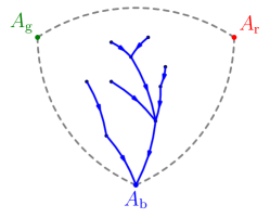
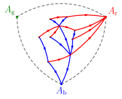
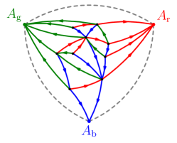
Figure 12. Construction from $w$ to the wooded triangulation $\psi(w)$: (a) draw the planar tree $\mathcal{M}_{\mathrm{b}}$; (b) draw $\mathcal{M}_{\mathrm{b}\mathrm{r}}$ in a planar way as in Proposition 2.3; (c) finally, the green edges triangulate each face in Figure 12(b) in the manner of Figure 11(b).

By Lemma 2.4, each inner face in $\mathcal{M}_{\mathrm{b}\mathrm{r}}$ is of the form in Figure 11(a). Namely, there is a unique blue (resp., red) edge so that the face is left (resp., right) of that edge. Let $\overline{\mathcal{M}}_{\mathrm{b}\mathrm{r}}:=\mathcal{M}_{\mathrm{b}\mathrm{r}}\cup\{\overline{A_{\mathrm{g}}A_{\mathrm{b}}},\overline{A_{\mathrm{g}}A_{\mathrm{r}}}\}$. We can embed $\overline{\mathcal{M}}_{\mathrm{b}\mathrm{r}}$ so that $\overline{A_{\mathrm{b}}A_{\mathrm{r}}},\overline{A_{\mathrm{g}}A_{\mathrm{b}}},\overline{A_{\mathrm{g}}A_{\mathrm{r}}}$ form the unbounded face of $\overline{\mathcal{M}}_{\mathrm{b}\mathrm{r}}$. Let $f_{\mathrm{b}\mathrm{r}}$ be the inner face of $\overline{\mathcal{M}}_{\mathrm{b}\mathrm{r}}$ containing $A_{\mathrm{g}}$. To understand the structure of $f_{\mathrm{b}\mathrm{r}}$, let $w^{\prime}\in\mathcal{W}_{n+1}$ be the concatenation of g,b, $w$, and $\mathrm{r}$. If we identify $\overline{A_{\mathrm{g}}A_{\mathrm{b}}}$ (resp., $\overline{A_{\mathrm{g}}A_{\mathrm{r}}}$) as a blue (resp., red) directed edge, then $\overline{\mathcal{M}}_{\mathrm{b}\mathrm{r}}$ is isomorphic to $\mathcal{M}_{\mathrm{b}\mathrm{r}}(w^{\prime})$ and $f_{\mathrm{b}\mathrm{r}}$ becomes an inner face of $\mathcal{M}_{\mathrm{b}\mathrm{r}}(w^{\prime})$, thus by Lemma 2.4 also has the form in Figure 11(a).

Proof of Theorem 1.4.

By Proposition 2.1, we have $\varphi(\mathcal{S}_{n})\subset\mathcal{W}_{n}$. For all $w\in\mathcal{W}_{n}$, Definition 2.2 constructs a combinatorial map $\psi(w)$. Now we show that $\psi(w)\subset\mathcal{S}_{n}$ and $\varphi(\psi(w))=w$, which will yield the surjectivity of $\varphi$.

According to the structure of inner faces in $\overline{\mathcal{M}}_{\mathrm{b}\mathrm{r}}$ above and Lemma 2.4, we can recover $\psi(w)$ by triangulating each inner face $f$ of $\overline{\mathcal{M}}_{\mathrm{b}\mathrm{r}}$ by green edges. When $f$ is an inner face of $\mathcal{M}_{\mathrm{b}\mathrm{r}}$, then vertices of $f$ are of the form $v,v_{0},v_{1},\cdots,v_{m+1}$ as in Lemma 2.4. In this case we add green edges from $\{v_{i}\}_{1\leq i\leq m}$ to $v$ provided $m>0$. If $f=f_{\mathrm{b}\mathrm{r}}$, we add green edges to $A_{g}$ in the same way. This shows that $\psi(w)$ is a triangulation. Moreover, by the cyclic order in Definition 2.2, $\psi(w)$ is a size-$n$ wooded triangulation. Knowing that $\psi(w)\in\mathcal{S}_{n}$, it is clear that the edge-symbol correspondence in Definition 2.2 is identical to the one defined by clockwise exploring the blue tree of $\psi(w)$ as in Section 1.3.

We are left to show that $\psi(\varphi(S))=S$ for all $S\in\mathcal{S}_{n}$. Let $w=\varphi(S)$. First of all, as mentioned in the proof of Lemma 2.3 , the Dyck word of $\mathcal{M}_{\mathrm{b}}(w)$ is $w_{\mathrm{g}\mathrm{b}}$. So we can identify $\mathcal{M}_{\mathrm{b}}(w)$ with $T_{\mathrm{b}}(S)$ since the Dyck word of $T_{\mathrm{b}}(S)$ is also $w_{\mathrm{g}\mathrm{b}}$. Under this identification, if $w_{k}$ is a b symbol, then the inner vertex of $\psi(w)$ corresponding to $w_{k}$ identifies with the tail of a blue edge in $S$ such that $w_{k}$ is given by $\mathcal{P}_{S}$’s second traversal of this blue edge. Second, for each inner vertex of $\psi(w)$ and $S$, consider the incoming (resp., outgoing) red edges as incoming (resp., outgoing) arrows attched at this vertex, as in the proof of Lemma 2.3. By Schnyder’s rule, the number of outgoing arrows at each inner vertex is one. Suppose $w_{i}$ is a b symbol and $w_{j}$ is the gb match of $w_{i}$. By Definition 2.2, $w_{i}$ corresponds to a blue edge in $\psi(w)$ as long as its tail, say, $v$. As mentioned in the proof of Lemma 2.3, the number of incoming red arrows attached to $v$ is the number of consecutive r symbols right before $w_{j}$ in $w$. On the other hand, by the definition of $\varphi$, $w_{i}$ comes from $\mathcal{P}_{S}$’s second traversal of a blue edge, say, $e$. Moreover, $\mathcal{P}_{S}$’s crossing of the incoming red edge at the tail of $e$ corresponds to the consecutive r symbols right before $w_{j}$ in $w$. Therefore the number of incoming red arrows at the tail of $e$ equals the number of consecutive r symbols right before $w_{j}$ in $w$. So the number of red (incoming and outgoing) arrows at each inner vertex of $S$ is the same as that for the corresponding inner vertex of $\psi(w)$. By Lemma 2.3, $T_{\mathrm{b}}(S)\cup T_{\mathrm{b}}(S)$ coincides with $\mathcal{M}_{\mathrm{b}\mathrm{r}}(w)$. Finally, the way to obtain $\psi(\varphi(S))$ from $\overline{\mathcal{M}}_{\mathrm{b}\mathrm{r}}$ by adding green edges as above is also the way to obtain $S$ from $T_{\mathrm{b}}(S)\cup T_{\mathrm{r}}(S)\cup\{\overline{A_{\mathrm{b}}A_{\mathrm{r}}},\overline{A_{\mathrm{r}}A_{\mathrm{g}}},\overline{A_{\mathrm{g}}A_{\mathrm{b}}}\}$. This yields $\psi(\varphi(S))=S$. ∎

2.2. Dual map, dual tree and counterclockwise exploration

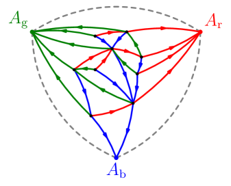
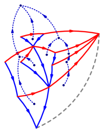
Figure 13. A Schnyder wood along with its dual blue tree and dual red tree.

In light of Theorem 1.4, we may apply the above constructions of $T_{\mathrm{b}},\overline{T}_{\mathrm{b}}$ and $\mathcal{M}_{\mathrm{b}\mathrm{r}}$ to obtain these planar maps for any $S\in\mathcal{S}_{n}$. Fix such an $S$, and note that $\overline{T}_{\mathrm{b}}$ is a spanning tree of $\mathcal{M}_{\mathrm{b}\mathrm{r}}$. We define a spanning tree on the dual map of $\mathcal{M}_{\mathrm{b}\mathrm{r}}$ (that is, the map of faces of $\mathcal{M}_{\mathrm{b}\mathrm{r}}$) rooted at the outer face by counterclockwise rotating each red edge. In other words, we form a directed edge from $F_{1}$ to $F_{2}$ if they are the faces on the right and left sides (respectively) of some directed red edge in $\mathcal{M}_{\mathrm{b}\mathrm{r}}$. We call this tree the dual blue tree of $S$.

We can define $T_{\mathrm{r}}$ and $\overline{T}_{\mathrm{r}}$ similarly to $T_{\mathrm{b}}$ and $\overline{T}_{\mathrm{b}}$ with $\mathrm{r}$ in place of $\mathrm{b}$. Then $\overline{T}_{\mathrm{r}}$ is also a spanning tree of $\mathcal{M}_{\mathrm{b}\mathrm{r}}$. By clockwise rotating each blue edge, we obtain the dual red tree of $S$. For any inner face $f$ of $\mathcal{M}_{\mathrm{b}\mathrm{r}}$, the branch on the dual blue tree from $f$ towards the dual root is called the dual blue flow line. We define the dual red flow line similarly with red in place of blue.

Recall the map $\mathcal{F}$ in Lemma 2.4. We extend $\mathcal{F}$ to the set of all inner edges as follows: let $\mathcal{F}(e)$ be the face of $\mathcal{M}_{\mathrm{b}\mathrm{r}}$ on the left of $e$ if $e$ is a blue or red edge; let $\mathcal{F}(e)$ be the face containing $e$ if $e$ is a green edge. We call $\mathcal{F}$ the face identification map. We also define $\widetilde{\mathcal{F}}(e)$ by replacing left with right in the definition of $\mathcal{F}(e)$.

Recall the exploration path $\mathcal{P}_{S}$ in the definition of $Z^{\mathrm{b}}$. By reversing the direction of $\mathcal{P}_{S}$ and swapping the roles of red and green edges, we can define a lattice walk $\prescript{\mathrm{b}}{}{Z}$ corresponding to the counterclockwise exploration of $T_{\mathrm{b}}$. More precisely, let $\widetilde{\mathcal{P}}_{S}$ be the time reversal of $\mathcal{P}_{S}$. Then $\prescript{\mathrm{b}}{}{Z}$ takes a $(1,-1)$-step if $\widetilde{\mathcal{P}}_{S}$ traverses a blue edge for the second time, a $(0,1)$-step (resp., $(-1,0)$-step) if $\widetilde{\mathcal{P}}_{S}$ crosses a red (resp., green) edge for the second time. We can similarly define $\prescript{\mathrm{r}}{}{Z}$ and $\prescript{\mathrm{g}}{}{Z}$ for the counterclockwise explorations of the red and green tree, respectively. Note that $\prescript{\mathrm{b}}{}{Z}$ is not the time reversal of $Z^{\mathrm{b}}$ in general. We introduce these counterclockwise walks because if we switch from clockwise exploration of $T_{\mathrm{b}}$ to the counterclockwise exploration and swap the roles of red and green, then $(Z^{\mathrm{b}},\mathcal{M}_{\mathrm{b}\mathrm{r}},\overline{T}_{\mathrm{b}},\textrm{ dual blue tree})$ becomes $(\prescript{\mathrm{r}}{}{Z},\mathcal{M}_{\mathrm{b}\mathrm{r}},\overline{T}_{\mathrm{r}},\textrm{ dual red tree})$. This symmetry will be important in Section 5. (Also see Proposition 2.5 below.)

Write $Z^{\mathrm{b}}=(L^{\mathrm{b}},R^{\mathrm{b}})$ and $\prescript{\mathrm{r}}{}{Z}=(\prescript{\mathrm{r}}{}{R},\prescript{\mathrm{r}}{}{L})$. The letters $R$ and $L$ are arranged in this way because $T_{\mathrm{b}}$ (resp., $T_{\mathrm{r}}$) is right (resp., left) of $\mathcal{P}_{S}$ (resp., $\widetilde{\mathcal{P}}_{S}$), while by Proposition 2.1, $R^{\mathrm{b}}$ (resp., $\prescript{\mathrm{r}}{}{L}$) is the contour function (modulo flat steps) of $T_{\mathrm{b}}$ (resp., $T_{\mathrm{r}}$).

To complete the mating-of-trees picture of our bijection $\varphi$, we now show that $L^{\mathrm{b}}$ and $\prescript{\mathrm{r}}{}{R}$ are contour functions (modulo flat steps) of the dual blue and dual red trees respectively.

Proposition 2.5.

In the above setting, for all $1\leq i\leq 3n$, $L^{\mathrm{b}}_{i}$ equals the number of edges on the dual blue flow line from $\mathcal{F}(w_{i})$ to the dual root.

The similar result holds for $\prescript{\mathrm{r}}{}{R}$, $\widetilde{\mathcal{F}}$, and dual red flow lines.

Proof.

It suffices to show that for all $1\leq k\leq 3n$, $L^{\mathrm{b}}_{k}-L^{\mathrm{b}}_{k-1}$ equals the difference between the number of edges on the dual blue flow lines starting from $\mathcal{F}(w_{k+1})$ and $\mathcal{F}(w_{k})$. When $w_{k}=\mathrm{r}$ (resp., $w_{k}=\mathrm{b}$), the face $\mathcal{F}(w_{k})$ is one step forward (resp., backward) along the dual blue flow line from $\mathcal{F}(w_{k-1})$. Moreover, $\mathcal{F}(w_{k})=\mathcal{F}(w_{k-1})$ when $w_{k}=\mathrm{g}$. Therefore the claim holds for each possible value of $w_{i}$. The result for $\prescript{\mathrm{r}}{}{R}$ follows by the symmetry of blue and red in $\mathcal{M}_{\mathrm{b}\mathrm{r}}$. ∎

2.3. Uniform infinite wooded triangulation

Thus far we have considered uniform samples from the set of all wooded triangulations of size $n$. We refer to this as the finite volume setting. In this section we introduce an infinite volume setting by defining an object which serves as the $n\to\infty$ limit of the uniform wooded triangulation of size $n$, rooted at a uniformly selected edge.

Let $\{w_{k}\,:\,1\leq k\leq 3n\}$ be a Markov chain on the state space $\{\mathrm{b},\mathrm{r},\mathrm{g}\}$ with $w_{1}=\mathrm{g}$ and transition matrix given by

(2.2) $$P=\hbox{}\vbox{\kern 0.86108pt\hbox{$\kern 0.0pt\kern 2.5pt\kern-5.0pt\left[\kern 0.0pt\kern-2.5pt\kern-5.55557pt\vbox{\kern-0.86108pt\vbox{\vbox{ \halign{\kern\arraycolsep\hfil\@arstrut$\kbcolstyle#$\hfil\kern\arraycolsep& \kern\arraycolsep\hfil$\@kbrowstyle#$\ifkbalignright\relax\else\hfil\fi\kern\arraycolsep&& \kern\arraycolsep\hfil$\@kbrowstyle#$\ifkbalignright\relax\else\hfil\fi\kern\arraycolsep\cr 5.0pt\hfil\@arstrut$\scriptstyle$\hfil\kern 5.0pt&5.0pt\hfil$\scriptstyle\mathrm{b}$\hfil\kern 5.0pt&5.0pt\hfil$\scriptstyle\mathrm{r}$\hfil\kern 5.0pt&5.0pt\hfil$\scriptstyle\mathrm{g}\\\mathrm{b}$\hfil\kern 5.0pt&5.0pt\hfil$\scriptstyle\frac{1}{2}$\hfil\kern 5.0pt&5.0pt\hfil$\scriptstyle\frac{1}{4}$\hfil\kern 5.0pt&5.0pt\hfil$\scriptstyle\frac{1}{4}\\\mathrm{r}$\hfil\kern 5.0pt&5.0pt\hfil$\scriptstyle 0$\hfil\kern 5.0pt&5.0pt\hfil$\scriptstyle\frac{1}{2}$\hfil\kern 5.0pt&5.0pt\hfil$\scriptstyle\frac{1}{2}\\\mathrm{g}$\hfil\kern 5.0pt&5.0pt\hfil$\scriptstyle\frac{1}{2}$\hfil\kern 5.0pt&5.0pt\hfil$\scriptstyle\frac{1}{4}$\hfil\kern 5.0pt&5.0pt\hfil$\scriptstyle\frac{1}{4}\\$\hfil\kern 5.0pt\crcr}}}}\right]$}}$$

Define $f:\{\mathrm{b},\mathrm{r},\mathrm{g}\}\to\mathbb{Z}^{2}$ by

(2.3) $$f(\mathrm{b})=(1,-1),\quad f(\mathrm{r})=(-1,0),\quad f(\mathrm{g})=(0,1).$$

Define the lattice walk $Z^{\mathrm{b},n}$ inductively by $Z^{\mathrm{b},n}_{0}=(0,0)$ and $Z^{\mathrm{b},n}_{k}-Z^{\mathrm{b},n}_{k-1}=f(w_{k})$ for $1\leq k\leq 3n$. The following proposition tells us that the law of $Z^{\mathrm{\mathrm{b},n}}$ may be mildly conditioned to obtain the uniform measure on $\mathcal{W}_{n}$.

Proposition 2.6.

The conditional law of $Z^{\mathrm{b},n}$ given $\{Z^{\mathrm{b},n}\in\mathcal{W}_{n}\}$ is the uniform measure on $\mathcal{W}_{n}$. Moreover,

(2.4) $$\mathbb{P}[Z^{\mathrm{b},n}\in\mathcal{W}_{n}]=\left(\tfrac{48}{\pi}+o_{n}(1)\right)n^{-5},$$

where $o_{n}(1)$ denotes a quantity tending to zero as $n\to\infty$.

Proof of Proposition 2.6.

We claim that for all walks $w\in\mathcal{W}_{n}$, we have $\mathbb{P}[Z^{\mathrm{b},n}=w]=2\cdot 16^{-n}$. To see this, write the transition matrix as

$$P=\frac{1}{4}\left[\begin{array}[]{ccc}2&1&1\\ 0&2&2\\ 2&1&1\end{array}\right].$$

For a word $w=w_{1}\cdots w_{3n}\in\mathcal{W}_{n}$,

$$\mathbb{P}[\mathrm{word}(Z^{\mathrm{b},n})=w]=\left(\frac{1}{4}\right)^{3n-1}2^{\#(\mathrm{g}\to\mathrm{b})}2^{\#(\mathrm{b}\to\mathrm{b})}2^{\#(\mathrm{r}\to\mathrm{g})}2^{\#(\mathrm{r}\to\mathrm{r})},$$

where $\#(\mathrm{r}\to\mathrm{b})$ denotes the number of integers $1\leq i<3n$ for which $(w_{i},w_{i+1})=(\mathrm{r},\mathrm{b})$, and similarly for the other expressions. Here we used the bijection between $\mathcal{S}_{n}$ and $\mathcal{W}_{n}$. The first two factors multiply to give $2^{n}$, since there are $n$ occurrences of $\mathrm{b}$ in $w$. Similarly, the last two factors multiply to give $2^{n-1}$, since there are $n$ occurrences of $\mathrm{r}$ in $w$, with one at the end. Multiplying these probabilities gives the desired result.

For the second part of the proposition statement, we use the formula (1.3) for the number of wooded triangulations of size $n$. Stirling’s formula implies that the right-hand side of (1.3) is asymptotic to $\tfrac{24}{\pi}n^{-5}16^{n}$. Applying the first part of the present proposition and Theorem 1.4 concludes the proof. ∎

Remark 2.7.

Consider a 2D Brownian motion whose covariance is $-\cos(4\pi/\kappa)$ as in Theorem 1.2. The probability that it stays in the first quadrant over the interval $[0,2n]$ and returns to the origin is of order $n^{-\frac{\kappa}{4}-1}$; see e.g. [17]. The Brownian motion is the limit of the lattice walk, therefore, the exponent $\alpha=5$ in Proposition 2.6 and (1.3) is related to $\kappa=16$ via the equation $\alpha=\frac{\kappa}{4}+1$. This also explains why for uniform spanning tree decorated map we have $\kappa=8$ and $\alpha=3$ [62]; and for a bipolar-oriented map we have $\kappa=12$ and $\alpha=4$ [37].

From now on we slightly abuse the notation and redefine $Z^{\mathrm{b},n}$ to be the conditioned walk in Proposition 2.6. Note that the stationary distribution for $P$ is the uniform measure on $\{\mathrm{b},\mathrm{r},\mathrm{g}\}$. Now we define a bi-infinite random word $w$ so that $\{w_{i}\}_{i\geq 0}$ has the law of the Markov chain $P$ starting from the stationary distribution. And we extend $w$ to $\mathbb{Z}_{<0}$ so that $\{w_{i}\}_{i\in\mathbb{Z}}$ is a stationary sequence. We set $Z^{\mathrm{b},\infty}_{0}=(0,0)$ and $Z^{\mathrm{b},\infty}_{k}-Z^{\mathrm{b},\infty}_{k-1}=f(w_{k})$ for all $k\in\mathbb{Z}$, where $f$ is defined as in (2.3).

Proposition 2.8.

In the above setting, let $U$ be a uniform element of $\{0,1,\ldots,3n-1\}$, independent of $Z^{\mathrm{b},n}$. Define the re-centered walk $\widetilde{Z}^{\mathrm{b},n}_{k}:=Z^{\mathrm{b},n}_{(k+U)}-Z^{\mathrm{b},n}_{U}$ for $-U\leq k\leq 3n-U$. Then $\widetilde{Z}^{\mathrm{b},n}$ converges locally to $Z^{\mathrm{b},\infty}$, in the sense that for any fixed $T$, the law of $\left.\widetilde{Z}^{\mathrm{b},n}\right|_{[-T,T]}$ converges as $n\to\infty$ to the law of $Z^{\mathrm{b},\infty}|_{[-T,T]}$.

Proof.

Since $\mathbb{P}[Z^{\mathrm{b},n}\in\mathcal{W}_{n}]$ has subexponential decay by Proposition 2.6, the result follows by Cramér’s theorem for Markov chains [13, 14]. We refer the reader to Section 4.2 of [62] for more details. ∎

It is straightforward to verify that the bi-infinite word $w$ satisfies the following:

1. the sub-word $w_{\mathrm{g}\mathrm{b}}$ obtained by dropping all $\mathrm{r}$’s in $w$ is a parenthesis matching a.s.

2. the sub-word $w_{\mathrm{b}\mathrm{r}}$ obtained by dropping all $\mathrm{g}$’s in $w$ is a parenthesis matching a.s.

3. every $r$ in $w$ is followed by an r or g but not a $\mathrm{b}$.

Knowing the three properties, we can construct a random infinite graph $S^{\infty}$ with colored directed edges as in Definition 2.2. Namely, we identify the b symbols in $w$ as vertices in $S^{\infty}$. Then using the edge identification rule (1)-(3) in Definition 2.2, we identify b, g, and r symbols in $w$ with blue, red and green directed edges on $S^{\infty}$. We call the edge $e_{0}$ corresponding to $w_{0}$ the root of $S^{\infty}$. Note that we don’t introduce $A_{\mathrm{b}},A_{\mathrm{r}},A_{\mathrm{g}}$ here because in the edge identification rule in Definition 2.2, the possibility when $A_{\mathrm{b}},A_{\mathrm{r}},A_{\mathrm{g}}$ are attached to a colored edge a.s. never occur. Moreover, we don’t define the ordering of edges around vertices at this moment since we don’t want to involve the technicality of infinite combinatorial maps. Therefore $S^{\infty}$ is not a map yet. However, Proposition 2.9 below will imply that $S^{\infty}$ naturally carries an infinite planar map structure and a Schnyder wood structure (that is, a 3-orientation).

We adapt the notion of Benjamini-Schramm convergence [3] to the setting of rooted graphs with colored directed edges: let $(S^{n})_{n\geq 0}$ be a sequence of random rooted graph with colored and directed edges. We say that $S^{n}\to S^{0}$ as $n\to\infty$ in the Benjamini-Schramm sense if for every colored and oriented rooted graph $T$ and every $r>0$, the probability that the radius-$r$ neighborhood of the root in $S^{n}$ is isomorphic to $T$ converges as $n\to\infty$ to the probability that the radius-$r$ neighborhood of the root in $S^{0}$ is isomorphic to $T$.

Proposition 2.9.

Let $S^{n}$ be a uniform wooded triangulation of size $n$ and $e_{n}$ be a uniformly and independently sampled inner edge. Then $(S^{n},e_{n})$ converges in the Benjamini-Schramm sense to $(S^{\infty},e_{0})$.

Figure 14. To prove Proposition 2.9, we use an alternating sequence of enclosing br and gb matches to identify a sequence of subgraphs $G_{1},G_{2}\cdots$. The green region is $G_{1}$ and the blue region is $G_{m^{\prime}}$.

Proof.

Let $w^{n}$ be the word corresponding to $S^{n}$ and $\widetilde{w}^{n}$ be $w_{n}$ recentered at $U_{n}\in\{1,\cdots,3n\}$ where $U_{n}$ is the index corresponding to $e_{n}$ (that is, $w^{n}_{U_{n}}=e_{n}$). Let $(\widetilde{w}^{n}_{j_{1}(n)},\widetilde{w}^{n}_{k_{1}(n)})$ be the br match with minimal $k_{1}(n)$ such that $j_{1}(n)<0<k_{1}(n)$. Let $(w_{j_{1}},w_{k_{1}})$ denote the br match in $w$ with minimal $k_{1}$ so that $j_{1}<0<k_{1}$. Then by Proposition 2.8, we can couple $w,\widetilde{w}^{n}$ so that $\widetilde{w}^{n}([j_{1}(n),k_{1}(n)])=w([j_{1},k_{1}])$ with probability $1-o_{n}(1)$. Let $G^{n}_{1}$ (resp., $G_{1}$) be the graph consisting of edges in $\widetilde{w}^{n}([j_{1}(n),k_{1}(n)])$ (resp., $w([j_{1},k_{1}])$). Then $G^{n}_{1}$ and $G_{1}$ can be coupled so as to be equal with probability $1-o_{n}(1)$. This also means that $G_{1}$ is a.s. planar.

We let $(w_{j_{m}},w_{k_{m}})$ be the br match in $w$ so that $j_{m}<0<k_{m}$ and $k_{m}$ is the $m$-th smallest such index. By examining the word $w_{\mathrm{b}\mathrm{r}}$, it is straightforward to verify that $k_{m}<\infty$ a.s. for all $m$. We define $G^{n}_{m}$ and $G_{m}$ similarly. Then $G^{n}_{m}$ and $G_{m}$ can be coupled so as to be equal with high probability. Therefore, $G_{m}$ is a.s. planar.

Now we claim that the graph distance $r_{m}$ from $e_{0}$ to $S^{\infty}\setminus G_{m}$ tends to $\infty$ a.s. Note that $S^{\infty}=\bigcup_{m=1}^{\infty}G_{m}$. This will conclude the proof. Since $r_{m}$ is a non-decreasing integer sequence, it suffices to show that for all $m$ we can find an $m^{\prime}>m$ such that $r_{m^{\prime}}>r_{m}$. We only explain this for $m=1$ since the general case is the same. By examining $w_{\mathrm{g}\mathrm{r}}$, it is easy to see that there are infinitely many gb matches of the form $(w_{i},w_{l})$ so that $i<0<l$. In particular, we can find one such that $i<j_{1}<k_{1}<l$. Let $m^{\prime}$ be such that $j_{m^{\prime}}<i<l<k_{m^{\prime}}$. We abuse notation and also define $i,l,m^{\prime}$ for $\widetilde{w}^{n}$ as for $w$. Then by the coupling result above, $i,l,m^{\prime}$ are well defined with probability $1-o_{n}(1)$. Moreover, by Schnyder’s rule and the COLOR algorithm, on the event that $i,l,m^{\prime}$ are well defined for $\widetilde{w}^{n}$, the graph $G^{n}_{1}$ is contained in the interior of $G^{n}_{m^{\prime}}$ in the sense that the graph distance from $G^{n}_{1}$ to $S^{n}\setminus G^{n}_{m^{\prime}}$ is positive. (See Figure 14 for an illustration.) In particular, $r_{m^{\prime}}>r_{1}$. ∎

Definition 2.10.

We call $(S^{\infty},e_{0})$ the rooted uniform infinite wooded triangulation, abbreviated to UIWT.

Let $w=\{w_{i}\}_{i\in\mathbb{Z}}$ be the stationary sequence associated to the Markov chain $P$. From proof of Proposition 2.9, a sample of $(S^{\infty},e_{0})$ can be obtained from $w$ as follows. We let $(w_{j_{m}},w_{k_{m}})$ be the br match in $w$ so that $j_{m}<0<k_{m}$ and $k_{m}$ is the $m$-th smallest such index. Let $G_{m}$ be the graph consisting of edges in $w([j_{m},k_{m}])$ as in Figure 14. Then $S^{\infty}=\bigcup_{m=1}^{\infty}G_{m}$ is a sample of UIWT. Let $Z^{\mathrm{b},\infty}_{0}=(0,0)$ and $Z^{\mathrm{b},\infty}_{k}-Z^{\mathrm{b},\infty}_{k-1}=f(w_{k})$ with $f$ in (2.3). Then $w$, $Z^{\mathrm{b},\infty}$, and $(S^{\infty},e_{0})$ determine each other a.s. We call $Z^{\mathrm{b},\infty}$ is the random walk encoding of $S^{\infty}$ associated with the clockwise exploration of the blue tree. Results in Section 2.1 and 2.2 have natural extensions to $(S^{\infty},e_{0})$. We can similarly define $Z^{\mathrm{r},\infty},Z^{\mathrm{g},\infty},\prescript{\mathrm{b}}{}{Z}^{\infty},\prescript{\mathrm{r}}{}{Z}^{\infty},\prescript{\mathrm{g}}{}{Z}^{\infty}$, and we obtain joint convergence for all of them:

Proposition 2.11.

Let $(S^{n},e_{n})$ be defined in Proposition 2.9. Recall Section 2.2. We have six walks $Z^{\mathrm{b},n},Z^{\mathrm{r},n},Z^{\mathrm{g},n}$, $\prescript{\mathrm{b}}{}{Z}^{n},\prescript{\mathrm{r}}{}{Z}^{n},\prescript{{}^{\mathrm{g}}}{}{Z}^{n}$ associated with different explorations of $S^{n}$. The tuple $(S^{n},e_{n},Z^{\mathrm{b},n},Z^{\mathrm{r},n},Z^{\mathrm{g},n},\prescript{\mathrm{b}}{}{Z}^{n}$,$\prescript{\mathrm{r}}{}{Z}^{n}$, $\prescript{\mathrm{g}}{}{Z}^{n})$ jointly converges to $(S^{\infty},e_{0},$ $Z^{\mathrm{b},\infty},Z^{\mathrm{r},\infty},$ $Z^{\mathrm{g},\infty},\prescript{\mathrm{b}}{}{Z}^{\infty},\prescript{\mathrm{r}}{}{Z}^{\infty},\prescript{\mathrm{g}}{}{Z}^{\infty})$ in law. Here the convergence of walks is in the re-centered sense as in Proposition 2.8.

Proof.

As $(S^{n},e_{n},Z^{\mathrm{b},n})$ converges to $(S^{\infty},e_{0},Z^{\mathrm{b},\infty})$, the path $\mathcal{P}_{S^{n}}$ also converges to a bi-infinite path $\mathcal{P}_{S^{\infty}}$. Since $\prescript{\mathrm{b}}{}{Z}^{n}$ is defined in terms of $\mathcal{P}_{S^{n}}$ in a local manner, we see that $(S^{n},e_{n},Z^{\mathrm{b},n},\prescript{\mathrm{b}}{}{Z}^{n})$ jointly converge to $(S^{\infty},e_{0},$ $Z^{\mathrm{b},\infty},\prescript{\mathrm{b}}{}{Z}^{\infty})$ in law. By the clockwise/counterclockwise symmetry, $(S^{\infty},e_{0})$ and $\prescript{\mathrm{b}}{}{Z}^{\infty}$ determine each other a.s. By the symmetry of the three colors, the same joint convergence holds for the red and green colors. Since $(S^{\infty},e_{0})$ determines $Z^{\mathrm{r},\infty}$, $Z^{\mathrm{b},\infty}$, $\prescript{\mathrm{r}}{}{Z}^{\infty}$, and $\prescript{\mathrm{g}}{}{Z}^{\infty}$, we have the joint convergence of everything as desired. ∎

Now for a UIWT, we can define the map $\mathcal{M}_{\mathrm{b}\mathrm{r}}$, which is the union of blue and red edges. Flow lines, dual flow lines and the face identification mappings $\mathcal{F}$ and $\widetilde{\mathcal{F}}$ can also be defined for a UIWT. And the results in Section 2.1 and 2.2 have straightforward extensions to UIWT. In particular, we will use the following corollary of Proposition 2.5 in Section 5.3.

Proposition 2.12.

In the above setting, write ${Z}^{\mathrm{b},\infty}=(L^{\mathrm{b},\infty},R^{\mathrm{b},\infty})$. For any $k_{1}<k_{2}$, let $F$ be the face in $\mathcal{M}_{\mathrm{b}\mathrm{r}}$ where the dual blue flow lines from $\mathcal{F}(w_{k_{1}})$ and $\mathcal{F}(w_{k_{2}})$ merge, which exists almost surely. Then the difference between the number of dual edges from $\mathcal{F}(w_{k_{2}})$ and $\mathcal{F}(w_{k_{1}})$ to $F$ equals $L^{\mathrm{b},\infty}_{k_{2}}-L^{\mathrm{b},\infty}_{k_{1}}$. The similar result holds for $\prescript{\mathrm{r}}{}{Z}^{\infty}$, $\widetilde{\mathcal{F}}$, and dual red flow lines.

We conclude this section by studying the number of incoming green edges at a vertex. Write $\mathrm{Geom}(\frac{1}{2})$ as a geometric random variable with success probability $\frac{1}{2}$ supported on $\mathbb{Z}_{>0}$.

Lemma 2.13.

Let $T$ be a stopping time for $w$ with the property that $w_{T}=\mathrm{b}$ almost surely. Then the number $G$ of incoming green edges incident to the vertex corresponding to $w_{T}$ is distributed as $\mathrm{Geom}(\frac{1}{2})-1$.

Furthermore, $G$ is measurable with respect to the sequence of symbols between $w_{T}$ and its $\mathrm{b}\mathrm{r}$ match.

Proof.

Note that Lemma 2.4 holds for the UIWT, by Proposition 2.9. In the language of (2.1), $G=|\mathcal{G}_{T}|$. Now the lemma follows from the strong Markov property of $Z^{\mathrm{b},\infty}$ and the fact that the transition probability from b to r and g to r are both $\frac{1}{2}$. ∎

3. Convergence of one tree

In this section we prove marginal convergence of the triple of random walks featured in Theorem 1.5. Throughout this section, we let $S^{n}$ be a uniform wooded triangulation of size $n$ and $S^{\infty}$ be a UIWT. Let $Z^{\mathrm{b},n},\prescript{\mathrm{b}}{}{Z}^{n},Z^{\mathrm{b},\infty},\prescript{\mathrm{b}}{}{Z}^{\infty}$ be defined as in Section 2.3. Let $w^{n}$ and $w$ be the words corresponding to $S^{n}$ and $S$.

The following observation is an immediate consequence of Proposition 2.6

Lemma 3.1.

Let $\mathfrak{t}^{n}(0)=1$. For $1\leq k<2n$, let $\mathfrak{t}^{n}(k)=\min\{i>\mathfrak{t}^{n}(k-1):w^{n}_{i}\neq\mathrm{r}\}$. Define $\mathcal{Z}^{\mathrm{b},n}_{k}\colonequals Z^{\mathrm{b},n}_{\mathfrak{t}(k)}-Z^{\mathrm{b},n}_{\mathfrak{t}(0)}$ for $0\leq k<2n$. Let $\mathcal{Z}^{\mathrm{b},n}_{2n}=(0,0)$. Then $(\mathcal{Z}^{n}_{k})_{0\leq k\leq 2n}$ is distributed as a $(2n)$-step random walk with i.i.d. increments of step distribution

$$\tfrac{1}{2}\delta_{(1,-1)}+\sum_{i=0}^{\infty}2^{-i-2}\delta_{(-i,1)}\quad\quad\textrm{(see Figure~{}\ref{fig:steps} (b) for an illustration of the steps)}$$

conditioned on starting and ending at the origin and staying in $\{(i,j)\in\mathbb{Z}^{2}:i\geq 0;j\geq-1\}$. We call $\mathcal{Z}^{\mathrm{b},n}$ the grouped-step walk of $Z^{\mathrm{b},n}$.

Proof.

Recall that $Z^{b,n}$ starts and ends at $(0,0)$ and stays in the closed first quadrant, so it must start with $(0,1)$ and end with $(-1,0)$. Then by the construction we see that $\mathcal{Z}^{\mathrm{b},n}$ must start and end at $(0,0)$ and stay in $\{(i,j)\in\mathbb{Z}^{2}:i\geq 0;j\geq-1\}$. According to (2.2) and Lemma 2.6, the increments of $\mathcal{Z}^{\mathrm{b},n}$ are i.i.d. with the distribution given in the lemma. ∎

We also would like to define the grouped-step walk for $Z^{\mathrm{b},\infty}$. However, care must be taken about where we start grouping red steps. The following lemma is straightforward to check.

Lemma 3.2.

Let $T$ be a forward stopping time (that is, a stopping time for the filtration $\sigma(\{w_{i}\}_{i\leq k})$) of $w$ so that $w_{T}=\mathrm{b}$ or $w_{T}=\mathrm{g}$ a.s. Let $\mathfrak{t}(0)=T$ and for all $k\geq 1$, let $\mathfrak{t}(k)=\min\{i>\mathfrak{t}(k-1):w_{i}\neq r\}$. Let $\mathcal{Z}_{k}=Z^{\mathrm{b},\infty}_{\mathfrak{t}(k)}-Z^{\mathrm{b},\infty}_{T}$ for all $k\geq 0$. Then $\mathcal{Z}$ is distributed as a random walk with i.i.d. increments distributed as $\tfrac{1}{2}\delta_{(1,-1)}+\sum_{i=0}^{\infty}2^{-i-2}\delta_{(-i,1)}$. We call $\mathcal{Z}$ the forward grouped-step walk of $Z^{\mathrm{b},\infty}$ viewed from $T$, and denote its law by $\mathbb{P}^{\infty}$.

Remark 3.3.

The increments $\{(\eta^{x}_{k},\eta^{y}_{k})\}_{k\geq 0}$ of $\mathbb{P}^{\infty}$ satisfy $\mathbb{E}[(\eta^{x}_{k},\eta^{y}_{k})]=(0,0)$, $\mathbb{E}(|\eta^{x}_{k}|^{2})=2$, $\mathbb{E}(|\eta^{y}_{k}|^{2})=1$, and $\mathrm{cov}(\eta^{x}_{k},\eta^{y}_{k})=-1$.

Remark 3.4.

The reason we use a random time $T$ to re-center is because otherwise we would not get the distribution $\mathbb{P}^{\infty}$. However, if we set $T=\min\{i\geq 3nt:w_{i}=b\}$, then the law of $T-3nt$ does not depend on $t$ and has an exponential tail. Therefore, when we consider scaling limit questions where all times are rescaled by $(3n)^{-1}$, we can effectively think of $(3n)^{-1}T$ as the deterministic constant $t$, even in the finite volume setting where we’re conditioning on the polynomially unlikely event $w^{n}\in\mathcal{W}_{n}$.

Lemma 3.5.

Let $\{X_{k}\}_{k\geq 1}$ be a sequence of i.i.d. random variables where $X_{1}$ distributed as $\mathrm{Geom}(\frac{1}{2})$ or $\mathrm{Geom}(\frac{1}{2})-1$ or $\mathfrak{t}(1)-\mathfrak{t}(0)$ in Lemma 3.2. Let $N_{t}=\inf\{n:\sum_{1}^{n}X_{i}\leq t\}$. Then

(3.1) $$\lim_{n\to\infty}\frac{N_{tn}}{tn}=\frac{1}{\mathbb{E}[X_{1}]}\quad\textrm{a.s. for all $t$ simultaneously}.$$

Moreover, there exist absolute constants $c_{1},c_{2}>0$ such that

(3.2) $$\mathbb{P}\left[{\color[rgb]{0,0,0}\max_{1\leq k\leq n}\left|\sum_{i=1}^{k}X_{i}-k\mathbb{E}[X_{1}]\right|}>\sqrt{n}\log n\right]\leq c_{1}n^{-c_{2}\log n}.$$

Proof.

Formula (3.1) follows from the renewal theorem for random variables with finite means, which works for all the three distributions. For (3.2), when $X_{1}=\mathrm{Geom}(\frac{1}{2})$ or $\mathrm{Geom}(\frac{1}{2})-1$, by known concentration results for geometric random variables (see e.g. [36, Theorem 2.1 and 3.1]), we have

(3.3) $$\mathbb{P}\left[\left|{\sum_{i=1}^{k}X_{i}-k\mathbb{E}[X_{1}]}\right|>\sqrt{n}\log n\right]\leq c_{1}n^{-c_{2}\log n}\quad{\textrm{for }1\leq k\leq n}.$$

When $X_{1}\overset{d}{=}\mathfrak{t}(1)-\mathfrak{t}(0)$ in Lemma 3.2, we have $\mathbb{P}[X_{1}=1]=\frac{3}{4}$ and $\mathbb{P}[X_{1}=i]=2^{-i-1}$ for $i\geq 2$. Therefore we can couple $Y=\mathrm{Geom}(\frac{1}{2})-1$ with $X_{1}$ such that $Y=X_{1}$ if $X_{1}\geq 2$,

$$\mathbb{P}[Y=0|X_{1}=1]=\frac{1}{2},\quad\textrm{and}\quad\mathbb{P}[Y=1|X_{1}=1]=\frac{1}{4}.$$

Write $X_{1}=Y+(X_{1}-Y)$. Then $|X_{1}-Y|\leq 2$, thus by Azuma-Hoeffding inequality $X_{1}-Y$ satisfies the concentration in (3.2). Therefore (3.2) holds for $X$ in all three cases. By the union bound we get (3.2) from (3.3) after possibly increasing $c_{1}$ and decreasing $c_{2}$. ∎

Remark 3.6.

Sums of the form of $\sum_{i=1}^{n}X_{i}$ in Lemma 3.5 frequently appear when dealing the scaling limits of UIWT and its associated walks. Lemma 3.5 allows us to replace $\sum_{i=1}^{n}X_{i}$ by $n\mathbb{E}[X_{1}]$. Since the error $n^{-c\log n}$ in (3.2) decays much faster than $\mathbb{P}[w^{n}\in\mathcal{W}_{n}]$, this replacement is still valid under the finite volume conditioning. We will apply this observation several times in Section 5.

Write $Z^{\mathrm{b},\infty}$ as $(L^{\mathrm{b},\infty},R^{\mathrm{b},\infty})$. By taking $T=\inf\{i\geq 0:w_{i}=b\}$ and applying (3.5) to $Z^{\mathrm{b},\infty}$ and $\mathcal{Z}$, we have that $\left(\tfrac{1}{\sqrt{4n}}L^{\mathrm{b},\infty}_{\lfloor 3nt\rfloor},\tfrac{1}{\sqrt{2n}}R^{\mathrm{b},\infty}_{\lfloor 3nt\rfloor}\right)_{t\geq 0}$ weakly converges to a Brownian motion $\mathscr{Z}$ satisfying (1.1). By the stationarity of $w$ we have that $\left(\tfrac{1}{\sqrt{4n}}L^{\mathrm{b},\infty}_{\lfloor 3nt\rfloor},\tfrac{1}{\sqrt{2n}}R^{\mathrm{b},\infty}_{\lfloor 3nt\rfloor}\right)_{t\in\mathbb{R}}$ weakly converges to a two-sided Brownian motion (which we still denote by $\mathscr{Z}$) with the same variance and covariance. We now explain that the scaling limit of the walk ${}^{\mathrm{b}}Z^{\infty}$ is the time reversal of the scaling limit of $Z^{\mathrm{b},\infty}$, although this relation does not hold at the discrete level.

Proposition 3.7.

Write $\prescript{\mathrm{b}}{}{Z}^{\infty}=(\prescript{\mathrm{b}}{}{R}^{\infty},\prescript{\mathrm{b}}{}{L}^{\infty})$. Then

$$\left(\tfrac{1}{\sqrt{4n}}L^{\mathrm{b},\infty}_{\lfloor 3nt\rfloor},\tfrac{1}{\sqrt{2n}}R^{\mathrm{b},\infty}_{\lfloor 3nt\rfloor}\right)_{t\in\mathbb{R}}\quad\textrm{and}\quad\left(\tfrac{1}{\sqrt{4n}}\prescript{\mathrm{b}}{}{R}^{\infty}_{\lfloor 3nt\rfloor},\tfrac{1}{\sqrt{2n}}\prescript{\mathrm{b}}{}{L}^{\infty}_{\lfloor 3nt\rfloor}\right)_{t\in\mathbb{R}}$$

jointly converges in law to the process $\mathscr{Z}$, defined above, and its time reversal.

Proof.

To show that the scaling limits of $Z^{\mathrm{b},\infty}$ and $\prescript{\mathrm{b}}{}{Z}^{\infty}$ are related by time reversal, it suffices by tightness to show that any subsequential limit $(\mathscr{Z},\widehat{\mathscr{Z}}\>\>)$ of the two processes has the property that $\mathscr{Z}$ and $\widehat{\mathscr{Z}}$ are time reversals of each other. In other words, we want to show that $\mathscr{Z}_{t}=\widehat{\mathscr{Z}}_{-t}$ a.s. for all $t$. Without loss of generality we take $t=1$.

The process $R^{\mathrm{b},\infty}$ over the interval $[0,3n]$, with flat steps excised, is equal to the contour function of the portion of the blue tree traced by $\mathcal{P}_{S}$ during that interval. Furthermore, by Lemma 3.5, the asymptotic effect of including the flat steps is to time-scale the contour function by a factor of $\tfrac{3}{2}$. Similarly, $\prescript{\mathrm{b}}{}{L}^{\infty}$ is asymptotically within $o_{n}(1)$ of the contour function of the same portion of the same tree (also time-scaled by a factor of $\tfrac{3}{2}$), but traced in reverse. Therefore, the ordinates of $\mathscr{Z}_{1}$ and $\widehat{\mathscr{Z}}_{-1}$ are equal.

It remains to show that the abscissas of $\mathscr{Z}_{1}$ and $\widehat{\mathscr{Z}}_{-1}$ are equal. Roughly speaking, the idea is to (i) observe that the former counts the discrepancy between unmatched b’s and r’s in the segment $w_{0}\cdots w_{n}$ of the word $w$, and (ii) show that the latter approximately counts the same. By definition, $L^{\mathrm{b},\infty}_{n}$ is equal to $|L\cap[1,3n]_{\mathbb{Z}}|-|R\cap[1,3n]_{\mathbb{Z}}|$, where $L$ is the set of integers $k\geq 1$ such that $(w_{j},w_{k})$ is a br match and $j<0$, and $R$ is the set of integers $j\leq 3n$ such that $(w_{j},w_{k})$ is a br match and $k>3n$. (The absolute value bars denote cardinality.)

For $j\geq 1$, suppose that $w_{q}$ is the $j$th least element of $L$ and define $G^{L}_{j}$ to be the set of all integers $k$ such that $w_{k}=\mathrm{g}$ and there exists $p$ so that $(w_{p},w_{q})$ is the innermost br match enclosing $w_{k}$ (in other words, it is the match with maximal $p$ among those satisfying $p<k<q$). Similarly, for $j\geq 1$, let $w_{p}$ be the $j$th largest element of $R$ and define $G^{R}_{j}$ to be the set of all integers $k$ such that $w_{k}=\mathrm{g}$ and the br match $(w_{p},w_{q})$ is the innermost one enclosing $w_{k}$. Let $G^{L}$ and $G^{R}$ be disjoint unions of these sets, as follows:

(3.4) $$G^{L}=G^{L}_{1}\cup\cdots\cup G^{L}_{|L\,\cap[1,3n]_{\mathbb{Z}}|}\quad\text{ and }\quad G^{R}=G^{R}_{1}\cup\cdots\cup G^{R}_{|R\,\cap[1,3n]_{\mathbb{Z}}|}$$

By Definition 2.2, $\prescript{\mathrm{b}}{}{R}^{\infty}_{-n}$ is equal to $|G^{L}|-|G^{R}|$ . By the measurability part of Lemma 2.13, $(|G^{L}_{j}|)_{j=1}^{\infty}$ and $(|G^{R}_{j}|)_{j=1}^{\infty}$ are i.i.d. random variables with distribution $\mathrm{Geom}(\frac{1}{2})-1$.

Since elements of $L$ and $R$ correspond to running infima of $L^{\mathrm{b},\infty}$ and its time reversal, respectively, we have $|L\cap[1,3n]_{\mathbb{Z}}|\leq\sqrt{n}\log n$ and $|R\cap[1,3n]_{\mathbb{Z}}|\leq\sqrt{n}\log n$ with probability $1-o_{n}(1)$. Combined with (3.4) and Lemma 3.5, we have $L^{\mathrm{b},\infty}_{3n}=\prescript{\mathrm{b}}{}{R}^{\infty}_{3n}+O(n^{1/4})$ with probability $1-o_{n}(1)$. This concludes the proof. ∎

We conclude this section with the finite-volume version of Proposition 3.7.

Proposition 3.8.

Write $Z^{\mathrm{b},n}=(L^{\mathrm{b},n},R^{\mathrm{b},n})$ and $\prescript{\mathrm{b}}{}{Z}^{n}=(\prescript{\mathrm{b}}{}{R}^{n},\prescript{\mathrm{b}}{}{L}^{n})$. Then

$$\left(\tfrac{1}{\sqrt{4n}}L^{\mathrm{b},n}_{\lfloor 3nt\rfloor},\tfrac{1}{\sqrt{2n}}R^{\mathrm{b},n}_{\lfloor 3nt\rfloor}\right)_{t\in[0,1]}\quad\textrm{and}\quad\left(\tfrac{1}{\sqrt{4n}}\prescript{\mathrm{b}}{}{R}^{n}_{\lfloor 3nt\rfloor},\tfrac{1}{\sqrt{2n}}\prescript{\mathrm{b}}{}{L}^{n}_{\lfloor 3nt\rfloor}\right)_{t\in[0,1]}$$

jointly converges in law to $\mathscr{Z}^{\mathrm{b}}$ defined in Theorem 1.5 and its time reversal.

Proof.

Let $\mathcal{Z}^{\mathrm{b},n}=(\mathcal{L}^{\mathrm{b},n},\mathcal{R}^{\mathrm{b},n})$ be the grouped-step walk of $Z^{\mathrm{b},n}$. By the invariance principle for random walks in cones (see, e.g., [17]) and Remark 3.3, $\left(\tfrac{1}{\sqrt{4n}}\mathcal{L}_{\lfloor 2nt\rfloor}^{\mathrm{b},n},\tfrac{1}{\sqrt{2n}}\mathcal{R}_{\lfloor 2nt\rfloor}^{\mathrm{b},n}\right)$ converges to $\mathscr{Z}^{b}$. By the step distribution of $\mathcal{Z}^{\mathrm{b},n}$, we have

(3.5) $$|Z^{\mathrm{b}}_{m}-\mathcal{Z}^{\mathrm{b},n}_{k-1}|\leq|\mathcal{Z}^{\mathrm{b},n}_{k}-\mathcal{Z}^{\mathrm{b},n}_{k-1}|\quad\textrm{for all }1\leq k\leq 3n\textrm{ and }\mathfrak{t}^{n}(k-1)\leq m<\mathfrak{t}^{n}(k).$$

Now the convergence of $\left(\tfrac{1}{\sqrt{4n}}L^{\mathrm{b},n}_{\lfloor 3nt\rfloor},\tfrac{1}{\sqrt{2n}}R^{\mathrm{b},n}_{\lfloor 3nt\rfloor}\right)_{t\in[0,1]}$ follows from Lemma 3.5 by setting $X_{1}=\mathfrak{t}(1)-\mathfrak{t}(0)$.

To show the joint convergence in Proposition 3.8, we note that the proof of Proposition 3.7 works here as well, except that we have to condition on the polynomially unlikely event $\{w^{n}\in\mathcal{W}_{n}\}$. As explained in Remark 3.6, the estimate (3.2) allows us to ignore this conditioning and the argument in Proposition 3.7 goes through. ∎

4. Multiple Peano curves and an excursion theory

In this section we review the necessary background in the continuum. We focus on the case $\kappa\in(0,2)$ since eventually we only need $\kappa=1$. Throughout the section, we set

(4.1) $$\gamma=\sqrt{\kappa}\in(0,\sqrt{2})\quad\textrm{and}\quad\kappa^{\prime}=16/\kappa>8.$$

4.1. SLE, LQG and the peanosphere theory

We review the peanosphere/mating-of-trees theory [15]. We closely follow Sections 3 and 4 of the recent survey [24]. We first recall the LQG area measure. Let $\mathfrak{h}$ be a variant of Gaussian free field (GFF) on the plane. The $\gamma$-LQG area measure $\mu_{\mathfrak{h}}$ is the random measure on the plane formally defined by $e^{\gamma\mathfrak{h}}\,dx\,dy$, which is made rigorous by a regularization and limiting procedure as in [16]. In this section we let $\mathfrak{h}$ be a particular variant of GFF on the complex plane $\mathbb{C}$, which is the field describing a LQG surface called the $\gamma$-quantum cone. In this case, the measure $\mu_{\mathfrak{h}}$ is conjectured to be the scaling limit of the volume measure of the natural infinite volume random planar map model in the $\gamma$-LQG universality class. For example, we conjecture that when $\gamma=1$, the measure $\mu_{\mathfrak{h}}$ is the scaling limit of the vertex counting measure of the UIWT under a conformal embedding. We will not recall the precise definition of $\gamma$-quantum cone and the construction of $\mu_{\mathfrak{h}}$, which can be found in [24, Section 3.4]. For the rest of the paper it suffices to know that $\mu_{\mathfrak{h}}$ is an almost surely infinite random measure on $\mathbb{C}$ such that Theorem 4.1 below holds.

We now recall the space-filling SLE following [24, Section 3.6.3]. Let $R\mathbb{D}=\{z\in\mathbb{C}:|z|<R\}$ with $R>0$. A chordal $\operatorname{SLE}_{\kappa^{\prime}}$ on $R\mathbb{D}$ from $-iR$ to $iR$ is a random non-self-crossing space-filling curve from $-iR$ to $iR$. We denote it by $\eta^{\prime}_{R}$ and parametrize it such that $\eta^{\prime}_{R}(0)=0$ and in each unit of time it traverses a region of Euclidean area 1. Then $\eta^{\prime}_{R}$ converges in law to a space-filling curve $\eta^{\prime}$ on $\mathbb{C}$ in the local uniform topology. The limiting curve $\eta^{\prime}$ modulo monotone reparametrization is called a whole plane space-filling $\operatorname{SLE}_{\kappa^{\prime}}$. Consider an independent coupling of the $\gamma$-quantum cone field $\mathfrak{h}$ and a whole-plane space-filling $\operatorname{SLE}_{\kappa}^{\prime}$ curve $\eta^{\prime}$, with $\kappa^{\prime}=16/\kappa$ and $\gamma=\sqrt{\kappa}$ as in (4.1). In Theorem 4.1, we will parametrize $\eta^{\prime}$ using $\mu_{\mathfrak{h}}$ such that

(4.2) $$\eta^{\prime}(0)=0\quad\textrm{and}\quad\mu_{\mathfrak{h}}(\eta^{\prime}([s,t]))=t-s\quad\textrm{for }s<t.$$

The curve $\eta^{\prime}$ has the following properties which does not depend on its parametrization, although we use the one in (4.2) for concreteness. First, $\lim_{t\to\pm\infty}|\eta^{\prime}(t)|=\infty$. Moreover, for $t\in\mathbb{R}$, the intersection of $\eta^{\prime}(-\infty,t]$ and $\eta^{\prime}[t,\infty)$ can be viewed as the union of two curves from $\eta(t)$ to $\infty$, which we denote by $\eta_{t}^{\mathrm{L}}$ and $\eta_{t}^{\mathrm{R}}$, respectively. We let $\eta_{t}^{\mathrm{L}}$ be the curve such that $\eta^{\prime}(-\infty,t]$ is on the left side of $\eta_{t}^{\mathrm{L}}$ and call $\eta_{t}^{\mathrm{L}}$ the left boundary of $\eta^{\prime}(-\infty,t]$. We call $\eta_{t}^{\mathrm{R}}$ the right boundary of $\eta^{\prime}(-\infty,t]$. Under our assumption that $\kappa\in(0,\sqrt{2})$, the following holds almost surely: for each $t\in\mathbb{R}$ the curves $\eta_{t}^{\mathrm{L}}$ and $\eta_{t}^{\mathrm{R}}$ are simple and they do not intersect except at their endpoints. According to [61, 15], under the independent coupling of $\mathfrak{h}$ and $\eta^{\prime}$, the field $\mathfrak{h}$ induces a length measure called the $\gamma$-quantum length on the left and right boundaries of $\eta^{\prime}(-\infty,t]$ for all $t\in\mathbb{R}$. Let $\mathscr{L}_{t}$ (resp. $\mathscr{R}_{t}$) be the net change of the quantum lengths of the left (resp. right) boundary of $\eta^{\prime}(-\infty,t]$ relative to $\eta^{\prime}(-\infty,0]$. The following mating-of-trees theorem proved in [15, 22] is the infinite volume version of Theorem 1.2:

Theorem 4.1.

$\mathscr{Z}=(\mathscr{L},\mathscr{R})_{t\in\mathbb{R}}$ is a two-sided Brownian motion such that

(4.3) $$\operatorname{Var}[\mathscr{L}_{1}]=\operatorname{Var}[\mathscr{R}_{1}]=1\quad\textrm{and}\quad\operatorname{Cov}[\mathscr{L}_{1},\mathscr{R}_{1}]=-\cos\left(\frac{4\pi}{\kappa^{\prime}}\right),$$

Moreover, $\mathscr{Z}$ determines $(\mathfrak{h},\eta^{\prime})$ up to rotations.

Intuitively, the unit area $1$-LQG sphere in Theorem 1.2 is the $1$-quantum cone conditioned on having mass 1. Various rigorous conditioning procedures are performed in [15, 50] to construct this object. Another construction appears in [10]. See [1] for their equivalence. The proof of Theorem 1.2 in [50] is also via conditioning based on Theorem 4.1.

4.2. Imaginary geometry on LQG surfaces

Let $\eta^{\prime}$ be a whole-plane space-filling $\operatorname{SLE}_{\kappa^{\prime}}$. We first recall some distributional properties of $\eta^{\prime}$ as summarized in [24, Section 3.6.3]. For a fixed deterministic point $z\in\mathbb{C}$, almost surely there exists a unique time $t_{z}$ such that $\eta^{\prime}(t_{z})=z$. The law of the left boundary $\eta^{\mathrm{L}}_{t_{z}}$ and the right boundary $\eta^{\mathrm{R}}_{t_{z}}$ of $\eta^{\prime}(-\infty,t_{z}]$ have the same law, which is a variant of $\operatorname{SLE}_{\kappa}$ curve called the whole plane $\operatorname{SLE}_{\kappa}(2-\kappa)$ from $z$ to $\infty$. Conditioning on $\eta^{\mathrm{L}}_{t_{z}}$ and $\eta^{\mathrm{R}}_{t_{z}}$, the curves $\{\eta^{\prime}(t_{z}+s)\}_{s\geq 0}$ and $\{\eta^{\prime}(t_{z}-s)\}_{s\geq 0}$ evolve as two independent chordal $\operatorname{SLE}_{\kappa^{\prime}}$ from $z$ to $\infty$ on the two connected components of $\mathbb{C}\setminus(\eta^{\mathrm{L}}_{z}\cup\eta^{\mathrm{R}}_{z})$. The law of $\eta^{\prime}$ has time-reversal symmetry.

We now recall the basics of imaginary geometry [47, 48]. For $\kappa\in(0,2)$, let $\chi=2/\sqrt{\kappa}-\sqrt{\kappa}/2$. Fix $\theta\in(-\pi,\pi]$ and $z\in\mathbb{C}$. Consider the ordinary differential equation

(4.4) $$\dot{\eta}=e^{\frac{ih(\eta)}{\chi}+\theta},\quad\eta(0)=z.$$

If $h$ is a smooth function, then the initial-value problem has a unique solution. When $h$ is a variant of GFF, since $h$ is not pointwise defined, the equation (4.4) does not make literal sense. However, according to [47, 48] (in particular [48, Section 1.2.1]), there exists a coupling of a whole-plane $\operatorname{SLE}_{\kappa}(2-\kappa)$ curve $\eta_{z}^{\theta}$ from $z$ to $\infty$ and a particular variant of GFF called the whole-plane Gaussian free field modulo $2\pi\chi$, such that $(h,\eta_{z}^{\theta})$ can be interpreted as satisfying (4.4). We do not recall the definition of this particular variant of GFF and the full construction of this coupling, but only summarize the properties that are relevant to mating of trees. In this coupling $\eta_{z}^{\theta}$ is determined by $h$ a.s. We call $\eta_{z}^{\theta}$ the flow line of angle $\theta$ emanating from $z$. For each $\theta$, there exists a whole-plane space-filling $\operatorname{SLE}_{\kappa^{\prime}}$ curve $\eta^{\prime\theta}$ such that the following holds. For each fixed $z$, almost surely $\eta^{\mathrm{L}}_{t_{z}}$ (resp., $\eta^{\mathrm{R}}_{t_{z}}$) is the flow line of angle $\theta+\frac{\pi}{2}$ (resp., $\theta-\frac{\pi}{2}$) emanating from $z$. This uniquely characterizes a coupling of $(h,\eta^{\prime\theta})$ where $\eta^{\prime\theta}$ is a.s. determined by $h$. If $(h,\widetilde{\eta}^{\prime\theta})$ satisfies the same property, then we must have $\eta^{\prime\theta}=\widetilde{\eta}^{\prime\theta}$ almost surely. We call $\eta^{\prime\theta}$ the Peano curve for $h$ of angle $\theta$.

The three curves in the Theorem 1.5 are three Peano curves for the same $h$ with angle $0,\frac{2\pi}{3},\frac{4\pi}{3}$, respectively, where $\kappa=1$ and $\chi=\frac{3}{2}$. To prove Theorem 1.5, we need to understand the coupling between Peano curves of different angles. We first review the results from [23] on the coupling between one Peano curve and one flow line of an arbitrary angle. Suppose $\mathfrak{h}$ as in Theorem 4.1 and $h$ is a whole-plane GFF modulo $2\pi\chi$, which is independent of $\mathfrak{h}$. Suppose $\eta^{\prime}$ is the Peano curve for $h$ of angle $0$ so that $(\eta^{\prime},\mathfrak{h})$ are coupled independently as in Theorem 4.1. Parametrize $\eta^{\prime}$ by $\mu_{\mathfrak{h}}$ according to (4.2). Fix $\theta\in(-\frac{\pi}{2},\frac{\pi}{2})$. Let $\eta^{\theta}$ be the flow line of $h$ of angle $\theta$. Given $t\geq 0$, we say that $\eta^{\prime}$ crosses $\eta^{\theta}$ at time $t$ if and only if: (1) $\eta^{\prime}(t)$ is on the trace of $\eta^{\theta}$; (2) for each $\varepsilon>0$ there exists $s_{1},s_{2}\in(t-\varepsilon,t+\varepsilon)$ such that $\eta^{\prime}(s_{1})$ and $\eta^{\prime}(s_{2})$ lie on opposite sides of $\eta^{\theta}$. As explained in [23, Remark 3.1], when $\theta$ is such that $\eta^{\theta}$ does not intersect $\eta^{-\frac{\pi}{2}}$ and $\eta^{\frac{\pi}{2}}$, then $\eta^{\prime}$ crosses $\eta^{\theta}$ at time $t$ if and only if $\eta^{\prime}(t)$ is on the trace of $\eta^{\theta}$. When $\kappa=1$, this corresponds to $|\theta|\leq\frac{\pi}{6}$. The following proposition is extracted from [23, Propositions 3.2—3.4]. See Figure 15 for an illustration.

Figure 15. In Proposition 4.2, the point $\eta^{\prime}(t)$ may fall (a) left of the red flow line $\eta^{\theta}$ from $\eta^{\prime}(0)$, or (b) right of it.

Proposition 4.2.

For $\theta\in(-\frac{\pi}{2},\frac{\pi}{2})$, let $\mathcal{A}^{\theta}$ be the set of times when $\eta^{\prime}$ crosses $\eta^{\theta}$. Let $\mathscr{Z}$ be the two-sided Brownian motion determined by $(\eta^{\prime},\mathfrak{h})$ as in Theorem 4.1. For $t>0$, let $\widetilde{\tau}_{t}=\sup\{s\leq t:s\in\mathcal{A}^{\theta}\}$ and $\mathscr{W}_{t}=\mathscr{Z}_{t}-\mathscr{Z}_{\widetilde{\tau}_{t}}$. We have

1. $\mathcal{A}^{\theta}$ has the same distribution as the zero set of the standard Brownian motion.

2. For each $t>0$, $\mathscr{W}|_{[0,t]}$ and $\mathscr{Z}|_{[0,t]}$ almost surely determine each other. More precisely, they generate the same $\sigma$-algebra modulo null events.

3. Let $\ell^{\theta}$ be the Brownian local time of $\mathcal{A}^{\theta}$. There exists a deterministic constant $c>0$ such that for all $t>0$, the $\ell^{\theta}$-local time accumulated on $\{s\in[0,t]:\eta^{\prime}(s)\in\eta^{\theta}\}$ a.s.  equals $c$ times the quantum length of $\eta^{\theta}\cap\eta^{\prime}[0,t]$. (By [23, Lemma 3], $\eta^{\theta}\cap\eta^{\prime}[0,t)$ is a segment of $\eta^{\theta}$.)

We will describe the law of $\mathscr{W}$ in Section 4.3, for which we need the following lemma.

Lemma 4.3.

Let $p(\theta)$ be the probability that $\eta^{\prime}(1)$ lies on the right side of $\eta^{\theta}$, namely the region bounded by $\eta^{\theta}$ and the right frontier of $\eta^{\prime}(-\infty,0]$. Then $p$ is a homeomorphism between $(-\frac{\pi}{2},\frac{\pi}{2})$ and $(0,1)$ and therefore has an inverse function $\theta(p)$. Moreover, $p(\theta)+p(-\theta)=1$.

Proof.

By scaling, $p(\theta)$ also equals the probability that $\eta^{\prime}(t)$ lies on the right side of $\eta^{\theta}$ for any $t>0$. By Fubini’s theorem, $p(\theta)$ equals the expected $\mu_{\mathfrak{h}}$-area of the sub-region of $\eta^{\prime}[0,1]$ on the right side of $\eta^{\theta}$. Now the first statement follows from the monotonicity of flow lines with respect to angle [47] and the Monotone Convergence Theorem. The second statement follows from symmetry since the law of the image of $(\eta^{\prime},\eta^{\theta},\mu_{\mathfrak{h}})$ under the reflection $z\mapsto\bar{z}$ is that of $(\eta^{\prime},\eta^{-\theta},\mu_{\mathfrak{h}})$. ∎

4.3. A Poisson point process on half-plane Brownian excursions

For $\alpha\in(-1,1)$, let $\mathscr{Z}=(\mathscr{L},\mathscr{R})$ be a two-dimensional Brownian motion with covariance matrix

(4.5) $$\left(\begin{array}[]{cc}1&\alpha\\ \alpha&1\end{array}\right)$$

In this section we describe an excursion decomposition of $\mathscr{Z}$ which is the peanosphere counterpart of the theory in Section 4.2. It is implicitly developed in [23, Section 3], but we formulate it here via excursion theory. We will use this machinery to decompose $\mathcal{Z}^{\mathrm{b}}$ into excursions away from the red flow line from the root. This excursion description of the coupling of the blue Peano curve with red flow lines is a key tool in the proof of Theorem 1.5.

For topological spaces $A$ and $B$, we denote by $C(A,B)$ the set of continuous functions from $A$ to $B$. Given $\omega\in C(\mathbb{R}_{+},\mathbb{R})$, we define the infimum process $I(\omega)$ by $I(\omega)_{t}=\inf\{\omega_{s}:s\in[0,t]\}$. For $\ell\geq 0$, we define the hitting and crossing times $\tau^{-}(\omega)$ and $\tau(\omega)$ of $-\ell$:

(4.6) $$\tau^{-}(\omega)_{\ell}=\inf\{t:I(\omega)_{t}=-\ell\}\quad\textrm{and}\quad\tau(\omega)_{\ell}=\inf\{t:I(\omega)_{t}<-\ell\}.$$

Suppose $(B_{t})_{t\geq 0}$ is a standard one dimensional Brownian motion. By Levy’s theorem,then $B-I(B)$ has the same law as the reflected Brownian motion $|B|$. Let $e_{\ell}(t)$ be $B_{\tau^{-}(B)_{\ell}+t}-B_{\tau^{-}(B)_{\ell}}$ if $0\leq t\leq\tau(B)_{\ell}-\tau^{-}(B)_{\ell}$ and 0 otherwise. Then $(e_{\ell}(t)\,:\ell\geq 0)$ is a Poisson point process. We denote its intensity by $ds\otimes\mathbf{n}$ where $ds$ is the Lebesgue measure on $[0,\infty)$ and $\mathbf{n}$ is an infinite measure on $C(\mathbb{R}_{+},\mathbb{R})$. In this construction $(B_{t})_{t\geq 0}$, $B-I(B)$, and $(e_{\ell}:\ell\geq 0)$ determine each other. We call $I(B)$ the local time process of $B-I(B)$. We call $\mathbf{n}$ Ito’s excursion measure for $B-I(B)$. See e.g. [56, Chapter 13] for more background on the excursion theory.

Now let $\mathscr{Z}^{1}=(\mathscr{L}^{1},\mathscr{R}^{1})$ and $\mathscr{Z}^{0}=(\mathscr{L}^{0},\mathscr{R}^{0})$ be two independent copies of the 2D Brownian motion $\mathscr{Z}$ with covariance matrix (4.5). Let

(4.7) $$e^{1}_{\ell}(t)=\left\{\begin{array}[]{ll}\mathscr{Z}^{1}_{\tau^{-}(\mathscr{L}^{1})_{\ell}+t}-\mathscr{Z}^{1}_{\tau^{-}(\mathscr{L}^{1})_{\ell}},&\textrm{if}\;0\leq t\leq\tau(\mathscr{L}^{1})_{\ell}-\tau^{-}(\mathscr{L}^{1})_{\ell};\\ 0&\textrm{if}\;t>\tau(\mathscr{L}^{1})_{\ell}-\tau^{-}(\mathscr{L}^{1})_{\ell}.\end{array}\right.$$

and

(4.8) $$e^{0}_{\ell}(t)=\left\{\begin{array}[]{ll}\mathscr{Z}^{0}_{\tau^{-}(\mathscr{R}^{0})_{\ell}+t}-\mathscr{Z}^{0}_{\tau^{-}(\mathscr{R}^{0})_{\ell}},&\textrm{if}\;0\leq t\leq\tau(\mathscr{R}^{0})_{\ell}-\tau^{-}(\mathscr{R}^{0})_{\ell};\\ 0&\textrm{if}\;t>\tau(\mathscr{R}^{0})_{\ell}-\tau^{-}(\mathscr{R}^{0})_{\ell}.\end{array}\right.$$

Then $(e^{1}_{\ell}(t)\,:\ell\geq 0)$ and $(e^{0}_{\ell}(t)\,:\,\ell\geq 0)$ are Poisson point processes with excursion spaces

$$E^{1} =\bigcup_{\zeta>0}\big{\{}e=(x,y)\in C([0,\zeta],\mathbb{R}^{2})\,:\,e(0)=(0,0)\text{ and }x(\zeta)=0\text{ and }\left.x\right|_{(0,\zeta)}>0\big{\}},\text{ and}$$

$$E^{0} =\bigcup_{\zeta>0}\big{\{}e=(x,y)\in C([0,\zeta],\mathbb{R}^{2})\,:\,e(0)=(0,0)\text{ and }y(\zeta)=0\text{ and }\left.y\right|_{(0,\zeta)}>0\big{\}},$$

respectively. In words, $e^{1}$ (resp., $e^{0}$) is obtained from $\mathscr{Z}$ by keeping track of excursions in the right (resp., upper) half plane. As in the 1D case above, $\mathscr{Z}$ and $e^{1}$ determine each other. If we only keep the $x$-coordinate of excursions in $(e^{1}_{\ell}(t)\,:\ell\geq 0)$, we get a Poisson point process with the same law as $(e_{\ell}:\ell\geq 0)$ above. The same holds for $e^{0}$. In particular, the time set when the excursion occurs is distributed as the zero set of a 1D Brownian motion. Let $\mathbf{n}^{1}$ and $\mathbf{n}^{0}$ be the excursion measures for $e^{1}$ and $e^{0}$, respectively. Then for all $t>0$, $\mathbf{n}^{1}$ conditioned on $\zeta(e)>t$ equals the law of $\mathscr{Z}$ conditioned on staying in the right half plane during $[0,t]$. The same holds for $\mathbf{n}^{0}$ with the upper half plane in place of the right half plane. This specifies the measures $\mathbf{n}^{1}$ and $\mathbf{n}^{0}$ up to a multiplicative constant. We fix the constant by letting $\mathbf{n}^{1}(\zeta(e)>1)$ and $\mathbf{n}^{0}(\zeta(e)>1)$ equal to the corresponding quantity for the 1D excursion measure.

Now fix $p\in(0,1)$. For $\ell>0$, let $e^{p}{[0,\ell]}=e^{1}_{[0,p\ell]}\cup e^{0}_{[0,(1-p)\ell]}$. In words, $e^{p}$ is obtained by taking the union of $e^{1}$ and $e^{0}$ with their intensity diluted by a factor of $p$ and $1-p$, respectively. Then $e^{p}$ is the Poisson point process on $[0,\infty)\times(E^{1}\cup E^{0})$ with intensity $ds\otimes\mathbf{n}^{p}$ where $\mathbf{n}^{p}=p\mathbf{n}^{1}+(1-p)\mathbf{n}^{0}$. Thus we obtain a coupling $(e^{1},e^{0},e^{p},\mathscr{Z}^{1},\mathscr{Z}^{0})$, for which $(e^{1},\mathscr{Z}^{1})$ and $(e^{0},\mathscr{Z}^{0})$ are independent. Moreover, $(e^{1},e^{0})$ and $e^{p}$ determine each other.

We now recall the construction of a two dimensional Brownian motion $\mathscr{Z}^{p}$ out of $e^{p}$ from [23]. In contrast to the construction of $\mathscr{Z}^{1}$ out of $e^{1}$, we rely on imaginary geometry to stitch the excursions of $e^{p}$ together to form a Brownian motion $\mathscr{Z}^{p}$. Given $e\in E^{1}\cup E^{0}$, let $f(e)$ be the $x$-coordinate process of $e$ if $e\in E^{1}$ and the $y$-coordinate process of $e$ if $e\in E^{0}$. Then $f(e^{p}):=(f(e^{p}_{\ell})\,:\ell\geq 0)$ matches in law with the excursion process for $B-I(B)$ above. Therefore, we may define a reflected Brownian motion $\mathscr{X}^{p}$ such that the excursion process of $\mathscr{X}^{p}$ is $f(e^{p})$ (here a function $f$ on an excursion space is understood to act pointwise on the corresponding Poisson point process). For all $t>0$, let

$$\tilde{\tau}^{p}_{t}=\sup\{s:{\color[rgb]{0,0,0}\mathscr{X}^{p}_{s}}=0,s\leq t\},\quad\textrm{and}\quad\tau^{p}_{t}=\inf\{s:\mathscr{X}^{p}_{s}=0,s>t\}.$$

Let $(\ell^{p}_{t}\,:t\geq 0)$ be the local time process for $\mathscr{X}^{p}$. Namely, $(\ell^{p}_{t}\,:t\geq 0)$ is the local time process of a 1D Brownian motion $B$ such that $|B|=\mathscr{X}^{p}$. Then we can define a process $\mathscr{W}^{p}$ by requiring that $\mathscr{W}^{p}|_{[\tilde{\tau}^{p}_{t},\tau^{p}_{t}]}$ evolves as $e^{p}_{\ell^{p}_{t}}$ for all $t\geq 0$; namely $\mathscr{W}^{p}_{\tilde{\tau}^{p}_{t}+s}=e^{p}_{\ell^{p}_{t}}(s)$ for $s\in[0,\tau^{p}_{t}-\tilde{\tau}^{p}_{t}]$. Clearly, $\mathscr{W}^{p}$ is continuous on $\bigcup_{t}\,(\tilde{\tau}^{p}_{t},\tau^{p}_{t})$, and $\tilde{\tau}_{t}^{p}$ is the last discontinuity time of $\mathscr{W}^{p}$ before $t$, almost surely. We now recall [23, Proposition 3.2].

Proposition 4.4 ([23]).

The law of $\mathscr{W}^{p}$ is the same as that of $\mathscr{W}$ in Proposition 4.2 with $\theta=\theta(p)$, where $\theta(p)$ is as in Lemma 4.3.

By Proposition 4.2 (2), $\mathscr{W}^{p}$ determines a Brownian motion $\mathscr{Z}^{p}$. Then $\mathscr{W}^{p}$, $\mathscr{Z}^{p}$, and $e^{p}$ determine each other. We call $e^{p}$ the $p$-excursion of $\mathscr{Z}^{p}$. To summarize, we constructed a coupling of the following objects: $e^{1}$, $e^{0}$, $e^{p}$, $\mathscr{Z}^{1}$, $\mathscr{Z}^{0}$, $\mathscr{Z}^{p}$, $\mathscr{W}^{p}$, $\mathscr{X}^{p}$, and $\ell^{p}$. In this coupling, $\mathscr{Z}^{1}$ and $\mathscr{Z}^{0}$ are independent, and the dependence relations, expressed in terms of $\sigma$-algebras, are as follows:

(4.9) $$\sigma(e^{1})=\sigma(\mathscr{Z}^{1}),\sigma(e^{0})=\sigma(\mathscr{Z}^{0});$$

$$\sigma(e^{p})=\sigma(e^{0},e^{1})=\sigma(\mathscr{Z}^{p})=\sigma(\mathscr{W}^{p});$$

$$\sigma(\ell^{p})\subset\sigma(|\mathscr{X}^{p}|)\subset\sigma(\mathscr{Z}^{p}).$$

The following lemma gives a more explicit connection between $\mathscr{Z}^{1},\mathscr{Z}^{0},$ and $\mathscr{W}^{p}$.

Lemma 4.5.

We write $\mathscr{Z}^{1}=(\mathscr{L}^{1},\mathscr{R}^{1})$ and $\mathscr{Z}^{0}=(\mathscr{L}^{0},\mathscr{R}^{0})$. For $t\geq 0$, let $l_{t}=\sup\{a:{\color[rgb]{0,0,0}\tau^{-}(\mathscr{L}^{1})_{pa}+\tau^{-}(\mathscr{R}^{0})_{(1-p)a}}<t\}$. For each fixed $t\geq 0$, almost surely $\ell^{p}_{t}=l_{t}$ hence

$$\tilde{\tau}^{p}_{t}={\color[rgb]{0,0,0}\tau^{-}(\mathscr{L}^{1})_{pl_{t}}+\tau^{-}(\mathscr{R}^{0})_{(1-p)l_{t}}}\quad\textrm{and}\quad{\color[rgb]{0,0,0}\mathscr{W}^{p}_{\tilde{\tau}^{p}_{t}+s}=e^{p}_{l_{t}}(s)\quad\textrm{for }s\in[0,\tau^{p}_{t}-\tilde{\tau}^{p}_{t}]}.$$

Moreover, for each $t>0$, $e^{p}_{\ell_{t}}=e^{1}_{pl_{t}}$ with probability $p$ and $e^{p}_{\ell_{t}}=e^{0}_{(1-p)l_{t}}$ with probability $1-p$.

Proof.

By definition, $\tilde{\tau}^{p}_{t}=\sum_{\ell<\ell^{p}_{t}}\zeta(e^{p}_{\ell})=\sum_{\ell<p\ell^{p}_{t}}\zeta(e^{1}_{\ell})+\sum_{\ell<(1-p)\ell^{p}_{t}}\zeta(e^{0}_{\ell})$. Therefore $\tilde{\tau}^{p}_{t}=\tau^{-}(\mathscr{L}^{1})_{p\ell^{p}_{t}}+\tau^{-}(\mathscr{R}^{0})_{(1-p)\ell^{p}_{t}}$. Since $\tilde{\tau}^{p}_{t}<t$, we have $l_{t}\geq\ell^{p}_{t}$ a.s.

For a rational $\ell>\ell^{p}_{t}$, find another rational $\ell^{\prime}\in(\ell^{p}_{t},\ell)$. Then a.s. there is an excursion of $e^{p}$ in $(\ell^{\prime},\ell)$. Therefore ${\color[rgb]{0,0,0}\tau^{-}(\mathscr{L}^{1})_{p\ell}+\tau^{-}(\mathscr{R}^{0})_{(1-p)\ell}}>t$. This means $l_{t}\leq\ell$ hence $l_{t}\leq\ell^{p}_{t}$ a.s.

Note that $e^{p}_{\ell^{p}_{t}}\in e^{1}_{p\ell^{p}_{t}}\cup e^{0}_{(1-p)\ell^{p}_{t}}$ a.s. By the definition of $e^{p}$, we have $e^{p}_{\ell^{p}_{t}}\in E^{1}$ with probability $p$. Therefore $e^{p}_{\ell_{t}}=e^{1}_{pl_{t}}$ with probability $p$ and $e^{p}_{\ell_{t}}=e^{0}_{(1-p)l_{t}}$ with probability $1-p$. ∎

Definition 4.6.

For later reference, we define a random variable indicating the event described at the end of the statement of Lemma 4.5: $\delta(t)\colonequals 1$ if $e^{p}_{\ell_{t}}=e_{pl_{t}}^{1}$ and $\delta(t)\colonequals-1$ otherwise.

In Section 5.3, we will have a discrete analogue of the triple $(\mathscr{Z}^{1},\mathscr{Z}^{0},\mathscr{Z}^{p})$ for $\alpha=-\tfrac{\sqrt{2}}{2}$ and $p=\tfrac{\sqrt{2}}{1+\sqrt{2}}$ or $\tfrac{1}{1+\sqrt{2}}$ and establish weak convergence using a tightness plus uniqueness argument. The values of $p$ will be derived from the symmetry of the three trees in the Schnyder wood and the normalizing constants in the random walk scaling limit. Lemma 4.5 combined with the following characterization of the coupling $(\mathscr{Z}^{1},\mathscr{Z}^{0},\mathscr{Z}^{p})$ will help with the uniqueness part of the proof.

Lemma 4.7.

Consider $(\mathscr{Z}^{1},\mathscr{Z}^{0},\mathscr{Z}^{p})$ as coupled above (4.9), where $\mathscr{Z}^{p}$ is measurable with respect to $(\mathscr{Z}^{1},\mathscr{Z}^{0})$. Suppose in addition $\widetilde{\mathscr{Z}}^{p}$ is coupled with $(\mathscr{Z}^{1},\mathscr{Z}^{0})$ such that

1. $\widetilde{\mathscr{Z}}^{p}$ has the same law as $\mathscr{Z}^{0}$.

2. $\forall\,t>0$, $\widetilde{\mathscr{Z}}^{p}_{t}-\widetilde{\mathscr{Z}}^{p}_{\tilde{\tau}_{t}}=\mathscr{W}^{p}_{t}$ a.s. where $\tilde{\tau}$ and $\mathscr{W}^{p}$ are defined from $\mathscr{Z}^{0},\mathscr{Z}^{1}$ as in Lemma 4.5.

3. Both $\mathscr{Z}^{p}$ and $\widetilde{\mathscr{Z}}^{p}$ are $\mathcal{F}$-Brownian motions for $\mathcal{F}_{t}=\sigma((\mathscr{Z}^{p},\widetilde{\mathscr{Z}}^{p})|_{[0,t]})$.

Then $\widetilde{\mathscr{Z}}^{p}=\mathscr{Z}^{p}$.

Proof.

Note that $\tilde{\tau}_{t}$ is cádlág and $\mathscr{Z}^{p}$ is continuous. By considering rational $t$, we have that with probability 1, $\mathscr{Z}^{p}_{t}-\mathscr{Z}^{p}_{\tilde{\tau}_{t}}=\mathscr{W}^{p}_{t}$ for all $t$. Now Lemma 4.7 is an immediate consequence of [23, Lemma 3.17]. ∎

5. Joint convergence to three Peano curves

In Sections 5.1–5.3, we work in the infinite-volume setting. In the discrete, let $S^{\infty}$ be a UIWT as in Definition 2.10. Let $(Z^{\mathrm{b}},Z^{\mathrm{r}},Z^{\mathrm{g}})$ be the triple of lattice walks encoding of $S$ with respect to the clockwise explorations of its three spanning trees. In the continuum, recall the notations of Section 4.1. We assume $\kappa=\gamma=1$ and $\kappa^{\prime}=16$. Let $\mathfrak{h}$ be a field describing the $1$-LQG quantum cone. Let $h$ be a whole plane GFF modulo $2\pi\chi$ with $\chi=\frac{2}{\sqrt{\kappa}}-\frac{\sqrt{\kappa}}{2}$. Let $(\eta^{\mathrm{b}},\eta^{\mathrm{r}},\eta^{\mathrm{g}})$ be the Peano curves for $h$ of angle $(0,\tfrac{2\pi}{3},\tfrac{4\pi}{3})$ as defined below (4.4). For $\mathrm{c}\in\{\mathrm{b},\mathrm{r},\mathrm{g}\}$, let $\mathscr{Z}^{\mathrm{c},\infty}$ be the Brownian motion corresponding to $(\mu_{\mathfrak{h}},\eta^{\mathrm{c}})$ as descibed in Theorem 4.1. In Sections 5.1–5.3 we will prove the following Theorem 5.1, which infinite-volume version of Theorem 1.5. In the statement of Theorem 5.1 and throughout Sections 5.1–5.3, we we drop the supersript $\infty$ to simplify the notion. Namely, we write the UIWT $S^{\infty}$ as $S$, and write $(\mathscr{Z}^{\mathrm{c},\infty})_{t\in\mathbb{R}}$ as $(\mathscr{Z}^{\mathrm{c}})_{t\in\mathbb{R}}$.

Theorem 5.1.

In the above setting, write $Z^{\mathrm{b}}=(L^{\mathrm{b}},R^{\mathrm{b}}),Z^{\mathrm{r}}=(L^{\mathrm{r}},R^{\mathrm{r}}),Z^{\mathrm{g}}=(L^{\mathrm{g}},R^{\mathrm{g}})$. Then

$$\left(\tfrac{1}{\sqrt{4n}}L^{\mathrm{c}}_{\lfloor 3nt\rfloor},\tfrac{1}{\sqrt{2n}}R^{\mathrm{c}}_{\lfloor 3nt\rfloor}\right)_{t\in\mathbb{R}}\stackrel{{\scriptstyle\text{in law}}}{{\longrightarrow}}(\mathscr{Z}^{\mathrm{c}})_{t\in\mathbb{R}}\quad\textrm{for}\;\;\mathrm{c}\in\{\mathrm{b},\mathrm{r},\mathrm{g}\}.$$

and the convergence holds jointly for $(Z^{\mathrm{b}},Z^{\mathrm{r}},Z^{\mathrm{g}})$.

Remark 5.2 (Abuse of notation in the infinite volume setting).

Although $\mathscr{Z}^{\mathrm{c}}$ was also used in Theorem 1.5 to denote the limiting Brownian excursions from the finite volume setting, we believe this abuse of notation does not cause confusion since we will exclusively focus on the infinite volume setting in Sections 5.1–5.3. We will use $Z^{\mathrm{c},n}$ to denote the rescaled walks in Theorem 5.1. Although this notation is used in Section 2 and 3 to denote the unscaled walk in the finite volume case, for the same reason we believe this abuse of notation adds simplicity without causing confusion.

In Section 5.4, we use a conditioning argument to deduce Theorems 1.5 and 1.6 from Theorem 5.1. We now give an overview for the proof of Theorem 5.1, which occupies Sections 5.1–5.3. From Proposition 3.7 we already have the marginal convergence in Theorem 5.1, which in particular implies the tightness of the three walks. It suffices to show that in the subsequential limit the three Brownian motions are coupled as desired. From Section 4.3, we know that the second Brownian motion should be encoded by the first one through the local time for the left/right excursions of the first Peano curve, away flow lines coming from the frontier of the second Peano curve. In Section 5.1 we show that this local time encoding of quantum lengths for flow lines has an exact discrete analog for UIWT. In Section 5.2, we focus on one flow line coupled with the first Peano curve, and show that the random walks and local time processes from UIWT converge to their continuous counterpart as in Proposition 4.7. In Section 5.3 we put flow lines together to get the second Peano curve to show the joint convergence of the first two random walks. By symmetry we get the joint convergence of the three walks.

5.1. A decomposition of a one-dimensional random walk

Let $w$ be the stationary bi-infinite word associated with the UIWT $S$. For $i\in\mathbb{Z}$, let $\mathfrak{y}^{\mathrm{b}}(i)$ be the edge in $S$ corresponding to $w_{i}$. Then $(\mathfrak{y}^{b}(i))_{i\in\mathbb{Z}}$ can be thought of as the Peano curve exploring the blue tree of $S$. For any forward stopping time $T$ such that $w_{T}=\mathrm{b}$ a.s., recall the grouped-step walk $\mathcal{Z}$ defined in Lemma 3.2. We drop the dependence of $\mathcal{Z}$ on $T$ since the law of $\mathcal{Z}$ (namely $\mathbb{P}^{\infty}$) is independent of $T$ (Lemma 3.2).

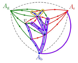
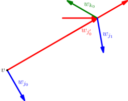
Figure 16. (a) A decomposition of the path $\mathcal{P}(S)$ into excursions right and left of the red flow line from a vertex $v$, shown in purple and gold, respectively. The corresponding decomposition of the word is as follows: $\color[rgb]{.5,.5,.5}{\mathrm{g}\mathrm{g}\mathrm{b}}{\color[rgb]{0.5,0,0.5}\underline{\mathrm{b}\mathrm{r}\mathrm{g}\mathrm{g}\mathrm{b}\mathrm{r}\mathrm{r}}}\>{\color[rgb]{0.7,0.7,0}\underline{\mathrm{g}\mathrm{g}\mathrm{b}\mathrm{r}\mathrm{g}\mathrm{b}}}\>{\color[rgb]{0.5,0,0.5}\underline{\mathrm{b}\mathrm{g}\mathrm{r}}}\>{\color[rgb]{0.7,0.7,0}\underline{\mathrm{g}}}\>{\color[rgb]{0.5,0,0.5}\underline{\mathrm{b}\mathrm{b}\mathrm{b}\mathrm{r}\mathrm{r}\mathrm{r}}}\mathrm{r}$. (b) An illustration of the symbols involved in the excursion decomposition of the word: $(w_{j_{0}},w_{j_{0}^{\prime}})$ is a br match, $w_{k_{0}}$ is the first $g$ after $w_{j_{0}^{\prime}}$ and $(w_{k_{0}},w_{j_{1}})$ is a gb match.

We now develop wooded-triangulation analogues of the objects featured in Sections 4.2 and 4.3. Similar discrete analogues have been considered in the bipolar orientation setting [23]. The forward and reverse explorations of a bipolar orientation are symmetric. However, they behave differently in the wooded triangulation setting considered below. We start from the forward exploration. Given a blue edge $\mathfrak{y}^{\mathrm{b}}(i)$ and its tail $v$, let $P_{i}$ be the red flow line from $v$. As a ray in a topological half plane bounded by the blue and green flow lines from $v$, the path $P_{i}$ admits a natural notion of left and right sides.

Lemma 5.3.

In the above setting, let $T$ be a forward stopping time such that $w_{T}=\mathrm{b}$ a.s. and let $\mathcal{Z}=(\mathcal{L},\mathcal{R})$ be the forward grouped-step walk viewed from $T$. Define a sequence $\sigma$ inductively by $\sigma_{0}=0$ and, for $i\geq 1$,

$$\sigma_{i} =\inf\{j>\sigma_{i-1}\,:\,\mathcal{L}_{j}<\mathcal{L}_{\sigma_{i-1}}\},\text{ if }i\text{ is odd,}$$

$$\sigma_{i} =\inf\{j>\sigma_{i-1}\,:\,\mathcal{R}_{j}<\mathcal{R}_{\sigma_{i-1}}\},\text{ if }i\text{ is even,}$$

Then for all integers $k\in[\mathfrak{t}(\sigma_{i}),\mathfrak{t}(\sigma_{i+1}-1)]$, the edge $\mathfrak{y}^{\mathrm{b}}(k)$ is right of the red flow line $P_{T}$ if $i$ is even and left of $P_{T}$ if $i$ is odd.

See Figure 17 for an illustration of the relationship between the excursion index $i$, the time index $j$ in $\mathcal{Z}$, and index $k$ considered in Lemma 5.3.

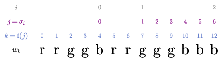
Figure 17. Three indices involved in Lemma 5.3 illustrated for a segment of a word.

Proof.

Beginning with $j_{0}\colonequals T$ (see Figure 16(b)), we perform the following algorithm :

1. Identify $w_{j_{0}}$’s br match $(w_{j_{0}},w_{j_{0}^{\prime}})$;

2. Let $k_{0}=\min\{k>j_{0}^{\prime}:w_{k}=g\}$;

3. Find $w_{k_{0}}$’s gb match $({w_{k_{0}}},w_{j_{1}})$;

4. Repeat, beginning with $j_{1}$ in place of $j_{0}$ to obtain $\{(j_{i},j^{\prime}_{i},k_{i})\}_{i\geq 0}$ iteratively.

According to Definition 2.2, the red edges $\mathfrak{y}^{\mathrm{b}}(j^{\prime}_{0}),\mathfrak{y}^{\mathrm{b}}(j^{\prime}_{1})\cdots$ form the red flow line $P_{T}$. Moreover, $\mathfrak{y}^{\mathrm{b}}$ is right (resp. left) of $P_{T}$ during $[j_{i},j^{\prime}_{i}-1]$ (resp. $[j^{\prime}_{i}+1,j_{i+1}-1]$) for all $i\geq 0$. Recall the sequence $\{\mathfrak{t}(k)\}_{k\geq 0}$ in Lemma 3.2. By the parenthesis matching rule, we have $j_{i}=\mathfrak{t}(\sigma_{2i})$ and $k_{i}=\mathfrak{t}(\sigma_{2i+1})$ for all $i\geq 0$. Therefore $w_{\mathfrak{t}(\sigma_{2i})}=\mathrm{b}$ and thus $\mathfrak{t}(\sigma_{2i}-1)=\mathfrak{t}(\sigma_{2i})-1$. Since $\mathfrak{t}(\sigma_{2i+1}-1)<j^{\prime}_{i}<k_{i}$, we conclude the proof. ∎

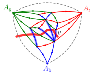
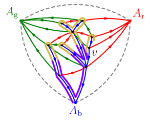
Figure 18. (a) The dual red flow line from $v$, which is obtained by starting from the face left of the outgoing blue edge from $v$. The corresponding sequence of blue edges is illustrated with the thick blue marker, and the path passing through all these edges is shown in red. (b) A decomposition according to the left and right excursions from the dual red flow line.

Definition 5.4.

For each $l\geq 0$, we call the walk $(\mathcal{Z}_{k}-\mathcal{Z}_{\sigma_{2l}})_{\sigma_{2l}\leq k\leq\sigma_{2l+1}}$ a right excursion and the walk $(\mathcal{Z}_{k}-\mathcal{Z}_{\sigma_{2l+1}})_{\sigma_{2l+1}\leq k\leq\sigma_{2l+2}}$ a left excursion.

Let ${\color[rgb]{0,0,0}\mathcal{T}^{1}(k)}=\sum_{0\leq l<k}(\sigma_{2l+1}-\sigma_{2l})$ and ${\color[rgb]{0,0,0}\mathcal{T}^{0}(j)}=\sum_{0\leq l<j}(\sigma_{2l+2}-\sigma_{2l+1})$. Let ${\color[rgb]{0,0,0}\mathcal{Z}^{1}=(\mathcal{L}^{1},\mathcal{R}^{1})}$ be the concatenation of right excursions. More precisely, let $\mathcal{Z}^{1}_{0}=(0,0)$. For $l\geq 0$ and $0\leq i\leq\sigma_{2l+1}-\sigma_{2l}$, let ${\color[rgb]{0,0,0}\mathcal{Z}^{1}_{i+\mathcal{T}^{1}(l)}-\mathcal{Z}^{1}_{\mathcal{T}^{1}(l)}}=\mathcal{Z}_{i+\sigma_{2l}}-\mathcal{Z}_{\sigma_{2l}}$. Let ${\color[rgb]{0,0,0}\mathcal{Z}^{0}=(\mathcal{L}^{0},\mathcal{R}^{0})}$ be the concatenation of left excursions defined in the same way.

When $\sigma_{2l}\leq n<\sigma_{2l+1}$ for some $l\geq 0$, let $(\mathcal{K}_{n},\mathcal{J}_{n})=(l,l)$. When $\sigma_{2l+1}\leq n<\sigma_{2l+2}$ for some $l\geq 0$, let $(\mathcal{K}_{n},\mathcal{J}_{n})=(l,l+1)$. We define the discrete local time of $\mathcal{Z}$ to be

$$\mathfrak{l}_{n}=-\inf_{m\leq\mathcal{T}^{1}(\mathcal{J}_{n})}\mathcal{L}^{1}_{m}-\inf_{m\leq{\mathcal{T}^{0}(\mathcal{K}_{n})}}\mathcal{R}^{0}_{m}.$$

By the strong Markov property, $\mathcal{Z}^{1}$ and $\mathcal{Z}^{0}$ are independent and equal in distribution to $\mathcal{Z}$. The process $(\mathcal{Z},\mathcal{Z}^{0},\mathcal{Z}^{1},\mathfrak{l})$ is a discrete analogue of $(\mathscr{Z}^{p},\mathscr{Z}^{0},\mathscr{Z}^{1},\ell^{p})$ in Lemma 4.5. (In fact, we will show in Section 5.2 that the scaling limit of the former is the latter with $p=\frac{\sqrt{2}}{1+\sqrt{2}}$.) Moreover, $\mathcal{J}_{n}-\mathcal{K}_{n}$ is the indicator of the event that $\mathcal{Z}$ reaches time $n$ during a left excursion, which is analogous to $\delta$ in Definition 4.6.

We have a similar story when considering the time reversal of $\mathfrak{y}^{\mathrm{b}}$ and dual red flow lines in $\mathcal{M}_{\mathrm{b}\mathrm{r}}$ (recall Section 2.3). Recall $Z^{\mathrm{b}}=(L^{\mathrm{b}},R^{\mathrm{b}})$.

Definition 5.5.

Let $T$ be a reverse stopping time of $w$, (that is, a stopping time with respect to the filtration $\mathcal{F}_{n}=\sigma(\{w_{i}\}_{i\geq n})$) such that $w_{T}=\mathrm{b}$ a.s. Let $\overline{\mathfrak{t}}(0)=T-1$ and for all $k\geq 1$, let $\overline{\mathfrak{t}}(k)=\max\{i<\overline{\mathfrak{t}}(k-1):w_{i}\neq r\}$. Let $\overline{\mathcal{L}}_{k}=R^{\mathrm{b}}_{\overline{\mathfrak{t}}(k)}-R^{\mathrm{b}}_{\overline{\mathfrak{t}}(0)}$ and $\overline{\mathcal{R}}_{k}=L^{\mathrm{b}}_{\overline{\mathfrak{t}}(k)}-L^{\mathrm{b}}_{\overline{\mathfrak{t}}(0)}$ for all $k\geq 0$. We call $\overline{\mathcal{Z}}:=(\overline{\mathcal{L}},\overline{\mathcal{R}})$ the reverse grouped-step walk $Z^{\mathrm{b}}$ viewed from $T$.

Note the interchange of $L$ and $R$, owing to the fact that reversing $\mathfrak{y}^{\mathrm{b}}$ swaps the notion of left and right (see the precise convention below). We drop the dependence of $\overline{\mathcal{Z}}$ on $T$ because the following lemma implies that the distribution of $\overline{\mathcal{Z}}$ is independent of $T$.

Lemma 5.6.

Let $\overline{\mathbb{P}}^{\infty}$ be the law of a random walk with i.i.d. increments distributed as $\tfrac{1}{2}\delta_{(1,-1)}+\sum_{i=0}^{\infty}2^{-i-2}\delta_{(-1,i)}$ (see Figure 7(c)). Then $\overline{\mathcal{Z}}$ is distributed as $\overline{\mathbb{P}}^{\infty}$.

Proof.

We have $w_{\overline{\mathfrak{t}}(0)}\neq\mathrm{r}$ a.s. because $w_{T}=\mathrm{b}$. If $w_{\overline{\mathfrak{t}}(0)}=\mathrm{b}$ we have $\overline{\mathcal{Z}}_{1}=(1,-1)$. If $w_{\overline{\mathfrak{t}}(0)}=\mathrm{g}$, then $\overline{\mathcal{L}}_{1}=-1$ and $\overline{\mathcal{R}}_{1}=\overline{\mathfrak{t}}(0)-\overline{\mathfrak{t}}(1)-1$. It is straightforward to check that the first increment of $\overline{\mathcal{Z}}$ has law indicated in Figure 7(c). A similar argument can be used to check the joint distribution of $\{\overline{\mathcal{Z}}_{k}-\overline{\mathcal{Z}}_{k-1}\}_{k\geq 1}$. ∎

The increments $\{(\eta^{x}_{k},\eta^{y}_{k})\}_{k\geq 0}$ of $\overline{\mathbb{P}}^{\infty}$ satisfy $\mathbb{E}[(\eta^{x}_{k},\eta^{y}_{k})]=(0,0)$, $\mathbb{E}(|\eta^{x}_{k}|^{2})=1$, $\mathbb{E}(|\eta^{y}_{k}|^{2})=2$, and $\mathrm{cov}(\eta^{x}_{k},\eta^{y}_{k})=-1$ (compare to Remark 3.3).

Given a blue edge $\mathfrak{y}^{\mathrm{b}}(i)$, its tail $v$ and the face $f=\mathcal{F}(\mathfrak{y}^{\mathrm{b}}(i))$ (recall Lemma 2.4), let $P^{\prime}_{i}$ be the dual red flow line starting from $f$. Since $P^{\prime}_{i}$ lives on the dual map of $\mathcal{M}_{\mathrm{b}\mathrm{r}}$, we have to be careful when talking about the left and right of $P^{\prime}_{i}$. Although particular choices do not matter in the scaling limit, for the sake of concreteness we fix the following convention. Given $P^{\prime}_{i}$, define the edge subset $\overline{P}_{i}$ of $S$ as follows: an edge $e$ is in $\overline{P}_{i}$ iff there is a blue edge $e^{\prime}$ such that $\mathcal{F}(e^{\prime})$ is on $P^{\prime}_{i}$ and $e$ is the next edge after $e^{\prime}$ when clockwise rotating around the tail of $e$. By Lemma 2.4, $\overline{P}_{i}$ is a simple path on $S$. As a ray in a topological half plane bounded by the blue and red flow lines from $v$, we have a natural notion of left and right for $\overline{P}_{i}$. For $k\leq 0$, we say $\mathfrak{y}^{\mathrm{b}}(k)$ is on the right of $P^{\prime}_{i}$ if $\mathfrak{y}^{\mathrm{b}}(k)$ lies on $\overline{P}_{i}$ or to its right. Otherwise we say $\mathfrak{y}^{\mathrm{b}}(k)$ is on the left of $P^{\prime}_{i}$. We have the following analogue of Lemma 5.3.

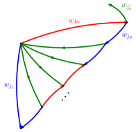
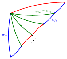
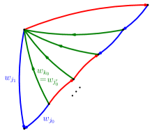
Figure 19. An illustration of one step of the iterative procedure in the proof of Lemma 5.7. We have the case $w_{j_{0}^{\prime}-1}=\mathrm{r}$ in (a), the case $w_{j_{0}^{\prime}-1}=\mathrm{g}$ in (b), and the case $w_{j_{0}^{\prime}-1}=\mathrm{b}$ in (c). In all three cases our proof of Lemma 5.7 works.

Lemma 5.7.

In the above setting, let $T$ be a reverse stopping time such that $w_{T}=\mathrm{b}$ almost surely, and let $\overline{\mathcal{Z}}$ be the reverse grouped-step walk viewed from $T$. Define a sequence $\overline{\sigma}$ inductively by $\overline{\sigma}_{0}=0$ and, for $i\geq 1$,

$$\overline{\sigma}_{i} =\inf\{j>\overline{\sigma}_{i-1}\,:\,\overline{\mathcal{L}}_{j}<\overline{\mathcal{L}}_{\overline{\sigma}_{i-1}}\}\text{ if }i\text{ is odd,}$$

$$\overline{\sigma}_{i} =\inf\{j>\overline{\sigma}_{i-1}\,:\,\overline{\mathcal{R}}_{j}<\overline{\mathcal{R}}_{\overline{\sigma}_{i-1}}\}\text{ if }i\text{ is even}.$$

Then for each $k\in[\overline{\mathfrak{t}}(\sigma_{i+1})+1,\overline{\mathfrak{t}}(\sigma_{i})]$, the edge $\mathfrak{y}^{\mathrm{b}}(k)$ is right of the dual red flow line $P^{\prime}_{T}$ if $i$ is even and left of $P^{\prime}_{T}$ if $i$ is odd.

Proof.

Beginning with $j_{0}\colonequals T$ (see Figure 18(c)), we perform the following algorithm.

1. Identify $w_{j_{0}}$’s gb match $(w_{j_{0}^{\prime}},w_{j_{0}})$

2. Let $k_{0}=\max\{k<j^{\prime}_{0}:w_{k}\neq r\}$+1.

3. Let $j_{1}=\max\{j<k_{0}:w_{j}=\mathrm{b},\;\textrm{and the br match $(w_{j},w_{\ell})$ satisfies}\;\ell\geq k_{0}\}$.

4. Repeat, beginning with $j_{1}$ in place of $j_{0}$ to obtain $\{(j_{i},k_{i})\}_{i\geq 0}$ iteratively.

By Definition 2.2 and Lemma 2.4, edges of $\overline{P}_{T}$ are exactly $\{\mathfrak{y}^{\mathrm{b}}(k_{i})\}_{i\geq 0}$ in order. Moreover, for $i\geq 0$, the edge $\mathfrak{y}^{\mathrm{b}}(k)$ is on the right of $P^{\prime}_{T}$ (according to the convention above) if $k_{i}\leq k<j_{i}$ and on the left of $P^{\prime}_{T}$ if $j_{i+1}\leq k<k_{i}$. Note that $Z^{\mathrm{b}}_{k}-Z^{\mathrm{b}}_{k-1}=f(w_{k})$. It can be checked by induction that $\bar{\mathfrak{t}}(\sigma_{2i+1})=k_{i}-1$ and $\bar{\mathfrak{t}}(\sigma_{2i})=j_{i}-1$ for all $i\geq 0$. This concludes the proof. ∎

We can define $(\overline{\mathcal{Z}},\overline{\mathcal{Z}}^{0},\overline{\mathcal{Z}}^{1},\overline{\mathfrak{l}})$ in the same way as $(\mathcal{Z},\mathcal{Z}^{0},\mathcal{Z}^{1},{\mathfrak{l}})$. The process $(\overline{\mathcal{Z}},\overline{\mathcal{Z}}^{0},\overline{\mathcal{Z}}^{1},\overline{\mathfrak{l}})$ is another discrete analogue of $(\mathscr{Z}^{p},\mathscr{Z}^{0},\mathscr{Z}^{1},\ell^{p})$ in Lemma 4.5. Although we need to analyze both $\mathcal{Z}$ and $\overline{\mathcal{Z}}$, the arguments will be almost identical. And as explained in Remark 5.8 below, $\mathcal{Z}$ offers slightly more technical challenges. So in Section 5.2 and 5.3 we treat $\mathcal{Z}$ in detail and $\overline{\mathcal{Z}}$ in brief.

Remark 5.8.

The right excursions of the flow line exhibit an overshoot phenomenon. More precisely, let $\Delta_{i}=\mathcal{L}_{\sigma_{2i-2}}-\mathcal{L}_{\sigma_{2i-1}}$ for $i\geq 1$. Then by the law $\mathbb{P}^{\infty}$ of $\mathcal{Z}$ described in Lemma 3.2, $\{\Delta_{i}\}_{i\geq 1}$ are i.i.d. with distribution $\mathrm{Geom}(\frac{1}{2})$. Meanwhile, the left excursions of the flow line and both left and right excursions of the dual flow line always hit $-1$ deterministically.

Finally, we note that although the discussion above is in the setting where we view the UIWT $S$ from a blue edge $e=\eta^{\mathrm{b}}(T)$, where $T$ is a forward or reverse stopping time, the combinatorial results are the same if we instead view $S$ from an arbitrary blue edge $e$ on the UIWT or on a finite wooded triangulation.

5.2. Joint convergence of a pair of trees and a flow line

Suppose we are in the setting of Section 5.1. Throughout this subsection, let the forward stopping time $T$ in Lemma 5.3 be $\min\{i\geq 0:w_{i}=b\}$ and the reverse stopping time $T$ in Lemma 5.7 be $\max\{i\leq 0:w_{i}=b\}$. Recall Definition 5.4. Let $(\mathcal{L}^{n}_{t})_{t\geq 0}$ and $(\mathcal{R}^{n}_{t})_{t\geq 0}$ be the linear interpolation of $\left(\frac{1}{\sqrt{4n}}\mathcal{L}_{2nt}\right)_{t\in\frac{1}{2n}\mathbb{N}}$ and $\left(\frac{1}{\sqrt{2n}}\mathcal{R}_{2nt}\right)_{t\in\frac{1}{2n}\mathbb{N}}$, respectively, and set $\mathcal{Z}^{n}_{t}=(\mathcal{L}^{n}_{t},\mathcal{R}^{n}_{t})$ for $t\geq 0$. We define $\mathcal{Z}^{0,n}_{t}=(\mathcal{L}^{0,n}_{t},\mathcal{R}^{0,n}_{t})$ and $\mathcal{Z}^{1,n}_{t}=(\mathcal{L}^{1,n}_{t},\mathcal{R}^{1,n}_{t})$ in the same way with $\mathcal{Z}^{0}$ and $\mathcal{Z}^{1}$ in place of $\mathcal{Z}$. Let

$$J^{n}_{t}=\mathcal{J}_{\lfloor 2nt\rfloor}\quad\textrm{and}\quad K^{n}_{t}=\mathcal{K}_{\lfloor 2nt\rfloor},$$

$$T^{1,n}(j)=(2n)^{-1}\mathcal{T}^{1}(j)\quad\textrm{and}\quad T^{0,n}(k)=(2n)^{-1}\mathcal{T}^{0}(k).$$

Let the rescaled local time of $\mathcal{Z}^{n}$ to be

(5.1) $$\mathfrak{l}^{\,n}_{t}=-\inf_{s\leq T^{1,n}(J_{t})}\mathcal{L}^{1,n}_{s}-\inf_{s\leq{T^{0,n}(K_{t})}}\mathcal{R}^{0,n}_{s}\quad\quad\forall\;t\geq 0.$$

We may also define the rescaled version of $(\overline{\mathcal{Z}},\overline{\mathcal{Z}}^{1},\overline{\mathcal{Z}}^{0},\overline{\mathfrak{l}})$, denoted by $(\overline{\mathcal{Z}}^{n},\overline{\mathcal{Z}}^{1,n},\overline{\mathcal{Z}}^{0,n},\overline{\mathfrak{l}}^{n})$. Since we swap $L$ and $R$ in the definition of $\overline{\mathcal{Z}}$, the scaling of the abscissa and ordinate is also swapped: $\overline{\mathcal{Z}}^{n}_{t}=\left(\frac{1}{\sqrt{2n}}\overline{\mathcal{L}}_{2nt},\frac{1}{\sqrt{4n}}\overline{\mathcal{R}}_{2nt}\right)$. We also adapt the scaling for $\overline{\mathcal{Z}}^{1,n},\overline{\mathcal{Z}}^{0,n},\overline{\mathfrak{l}}^{n}$ accordingly.

Proposition 5.9.

In the above setting, the triple $\left(\tfrac{1}{\sqrt{4n}}L^{\mathrm{b}}_{\lfloor 3nt\rfloor},\tfrac{1}{\sqrt{2n}}R^{\mathrm{b}}_{\lfloor 3nt\rfloor}\right)_{t\in\mathbb{R}},(\mathcal{Z}^{n}_{t})_{t\geq 0},$ and $(\overline{\mathcal{Z}}^{n}_{t})_{t\geq 0}$ jointly converge in law. Write $\mathscr{Z}^{\mathrm{b}}=(\mathscr{L}^{\mathrm{b}},\mathscr{R}^{\mathrm{b}})$ in Theorem 5.1. Then the joint limit of the triple is $(\mathscr{Z}^{\mathrm{b}}_{t})_{t\in\mathbb{R}}$, $(\mathscr{Z}^{\mathrm{b}}_{t})_{t\geq 0}$ and $(\mathscr{R}^{\mathrm{b}}_{-t},\mathscr{L}^{\mathrm{b}}_{-t})_{t\geq 0}$.

Proof.

By Proposition 3.7, $\left(\tfrac{1}{\sqrt{4n}}L^{\mathrm{b}}_{\lfloor 3nt\rfloor},\tfrac{1}{\sqrt{2n}}R^{\mathrm{b}}_{\lfloor 3nt\rfloor}\right)_{t\in\mathbb{R}}$ converges to $(\mathscr{Z}^{\mathrm{b}}_{t})_{t\in\mathbb{R}}$. By the proof of Proposition 3.7 based on Lemma 3.5, $\left(\tfrac{1}{\sqrt{4n}}L^{\mathrm{b}}_{\lfloor 3nt\rfloor},\tfrac{1}{\sqrt{2n}}R^{\mathrm{b}}_{\lfloor 3nt\rfloor}\right)_{t\in\mathbb{R}}$ and $(\mathcal{Z}^{n}_{t})_{t\geq 0}$ jointly converge to $(\mathscr{Z}^{\mathrm{b}}_{t})_{t\in\mathbb{R}}$ and $(\mathscr{Z}^{\mathrm{b}}_{t})_{t\geq 0}$. The same concentration in Lemma 3.5 also applies to the reverse grouped-step walks, which shows that $\left(\tfrac{1}{\sqrt{4n}}L^{\mathrm{b}}_{\lfloor 3nt\rfloor},\tfrac{1}{\sqrt{2n}}R^{\mathrm{b}}_{\lfloor 3nt\rfloor}\right)_{t\in\mathbb{R}}$ and $(\overline{\mathcal{Z}}^{n}_{t})_{t\geq 0}$ jointly converge to $(\mathscr{Z}^{\mathrm{b}}_{t})_{t\in\mathbb{R}}$ and $(\mathscr{R}^{\mathrm{b}}_{-t},\mathscr{L}^{\mathrm{b}}_{-t})_{t\geq 0}$. ∎

The key to the proof of Theorem 5.1 is the following:

Proposition 5.10.

With respect to the topology of uniform convergence on compact sets, $(\mathcal{Z}^{1,n},\mathcal{Z}^{0,n},\mathcal{Z}^{n},\mathfrak{l}^{n})$ jointly converges in law to $(\mathscr{Z}^{1},\mathscr{Z}^{0},\mathscr{Z}^{p},\ell^{p})$ defined in Section 4.3, with $\alpha=-\tfrac{\sqrt{2}}{2}$ and $p=\tfrac{\sqrt{2}}{1+\sqrt{2}}$. Furthermore, in any coupling such that the convergence is almost sure, for any fixed $t\in\mathbb{R}$, we have that $J^{n}_{t}-K^{n}_{t}$ converges to $\mathbf{1}_{\{\delta(t)=1\}}$ a.s., where $\delta(t)$ is the random variable defined in Definition 4.6. The same is true for $(\overline{\mathcal{Z}}^{n},\overline{\mathcal{Z}}^{1,n},\overline{\mathcal{Z}}^{0,n},\overline{\mathfrak{l}}^{n})$.

We begin with two lemmas. Recall the notation $\tau^{-}(\cdot)_{a}$ from (4.7). The first lemma is a standard fact about Brownian motion whose proof we will skip.

Lemma 5.11.

Suppose that $X^{n}$ is a sequence of stochastic process converging a.s. to a 1D standard Brownian motion $X^{0}$ in local uniform topology. Then for all $a>0$, we have $\tau^{-}(X^{n})_{a}$ converges to $\tau^{-}(X^{0})_{a}$ a.s. Furthermore, if we define $\sigma^{n}=\sup\{s\leq 1\,:\,X^{n}_{s}=\inf_{u\leq s}X^{n}_{u}\}$, then $\sigma^{n}\to\sigma^{0}$ a.s.

The second lemma is a 2D extension of Lemma 5.11.

Lemma 5.12.

Define $\widetilde{\tau}^{n}_{1}$ and $\tau_{1}^{n}$ to be the random times for which $(\widetilde{\tau}^{n}_{1},\tau_{1}^{n})$ is the largest open interval containing $t=1$ over which $t\mapsto\mathfrak{l}^{n}_{t}$ is constant. Then in any coupling such that $(\mathcal{Z}^{1,n},\mathcal{Z}^{0,n})_{n=1}^{\infty}$ converges to $(\mathscr{Z}^{1},\mathscr{Z}^{0})$ a.s., we have that $(\tilde{\tau}_{1}^{n},\tau_{1}^{n},\mathfrak{l}_{1}^{\,n},J^{n}_{1}-K^{n}_{1})$ converges to $(\tilde{\tau}_{1}^{p},\tau_{1}^{p},\ell^{p}_{1},\mathbf{1}_{\{\delta(1)=1\}})$ a.s., where $p=\tfrac{\sqrt{2}}{1+\sqrt{2}}$ and $\ell^{p}$ is as in Lemma 4.5.

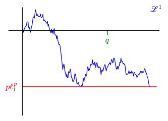
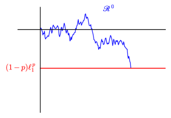
Figure 20. An illustration of the event $E=E^{i}_{q}$ when $i=1$. We lower the horizontal red lines in the two figures at rates $p$ and $1-p$, respectively, until the sum of the first hitting times exceeds $1$. The event $E$ occurs if this jump happens during an excursion of $\mathscr{L}^{1}$ including the time $q$ as shown.

Proof.

Recall that $\mathcal{Z}^{n}$ may be constructed from $(\mathcal{Z}^{1,n},\mathcal{Z}^{0,n})$ by alternately concatenating excursions, by the definition of $(\mathcal{Z}^{1,n},\mathcal{Z}^{0,n})$. After $2k$ such excursions have been concatenated ($k$ from $\mathcal{Z}^{1,n}$ and $k$ from $\mathcal{Z}^{0,n})$, the running infimum of the $\mathcal{R}^{0,n}$ is equal to $-k/\sqrt{2n}$, and the running infimum of $\mathcal{L}^{1,n}$ is $-(\Delta_{1}+\cdots+\Delta_{k})/\sqrt{4n}$, where $\{\Delta_{i}\}$ are the i.i.d. overshoots defined in Remark 5.8. Therefore, by Lemma 3.5,

(5.2) $$\lim_{n\to\infty}\frac{\mathcal{L}_{T^{1,n}(\lfloor a\sqrt{n}\rfloor)}^{1,n}}{\mathcal{R}_{T^{0,n}(\lfloor a\sqrt{n}\rfloor)}^{0,n}}=\frac{\mathbb{E}[\Delta_{1}]}{\sqrt{2}}={\color[rgb]{0,0,0}\sqrt{2}=\frac{p}{1-p}}\;\;\textrm{a.s. for all $a>0$ simultaneously.}$$

When $\delta(1)=1$ (resp. $\delta(1)=-1$), we have that $p\ell^{p}_{1}$ (resp. $(1-p)\ell^{p}_{1}$) is the global minimum of $\mathscr{L}^{1}$ (resp. $\mathscr{R}^{0}$) in $(0,T)$ for some $T>0$. For $q\in\mathbb{Q}_{>0}$, let $E^{1}_{q}$ the event that $\delta(1)=1$ and $p\ell^{p}_{1}$ is the global minimum of $\mathscr{L}^{1}|_{[0,q]}$. Let $E^{0}_{q}$ the event that $\delta(1)=-1$ and $(1-p)\ell^{p}_{1}$ is the global minimum of $\mathscr{R}^{0}|_{[0,q]}$. Then $\mathbb{P}[\bigcup_{i=0,1;\;q\in\mathbb{Q}_{>0}}E^{i}_{q}]=1$.

Let $E=E^{i}_{q}$ for some $i=0$ or 1 and $q\in\mathbb{Q}_{>0}$ such that $\mathbb{P}[E]>0$. For concreteness we may assume $i=1$ but the same argument works for $i=0$. (See Figure 20 for an illustration.) From now on we assume $E$ occurs. Let $a^{n}$ be such that $-pa^{n}\colonequals\min_{t\in[0,q]}\mathcal{L}^{1,n}_{t}$. Then since $(\mathcal{Z}^{1,n},\mathcal{Z}^{0,n})_{n=1}^{\infty}$ converge to $(\mathscr{Z}^{1},\mathscr{Z}^{0})$ a.s., Lemma 5.11 yields that $a^{n}\to\ell^{p}_{1}$ and $\tau^{-}(\mathcal{L}^{1,n})_{pa^{n}}\to\tau^{-}(\mathscr{L}^{1})_{p\ell^{p}_{1}}$ a.s. Let $j^{n}$ be the number of left excursions of $\mathcal{L}^{1}$ over the interal $[0,2qn]$. Then by Lemma 5.11,

$$T^{1,n}(j^{n})=\tau^{-}(\mathcal{L}^{1,n})_{pa^{n}}\to\tau^{-}(\mathscr{L}^{1})_{p\ell^{p}_{1}}\quad\textrm{and}\quad T^{1,n}(j^{n}+1)\to\inf\{t:\mathscr{L}^{1}_{t}<-p\ell^{p}_{1}\}\;\;\text{a.s.}$$

Let $k^{n}=j^{n}$. By (5.2) and the fact that $(1-p)\ell^{p}_{1}$ is a.s. a continuous point of $a\mapsto\tau^{-}(\mathscr{R}^{0})_{a}$, we have that ${\color[rgb]{0,0,0}T^{0,n}(k^{n})}\to\tau^{-}(\mathscr{R}^{0})_{(1-p)\ell^{p}_{1}}$.

Therefore, on the event $E$, for sufficiently large $n$ we have

$$T^{1,n}(j^{n})+T^{0,n}(k^{n})<1\quad\textrm{and}\quad T^{1,n}(j^{n}+1)+T^{0,n}(k^{n})>1\quad\text{ a.s.}$$

Recall the definition of $\mathfrak{l}^{n},J^{n}$ and $K^{n}$. We have $K^{n}_{1}=k_{n}$ and $J^{n}_{1}=j_{n}+1$. Therefore on $E$ we have that $(\tilde{\tau}_{1}^{n},\tau_{1}^{n},\mathfrak{l}_{1}^{\,n},J^{n}_{1}-K^{n}_{1})$ converges a.s. to $(\tilde{\tau}_{1}^{p},\tau_{1}^{p},\ell^{p}_{1},\mathbf{1}_{\delta(1)=1})$ as desired. Letting $E$ range over all the events $E^{i}_{q}$, we conclude the proof. ∎

Proof of Proposition 5.10.

We begin by showing joint convergence of $(\mathcal{Z}^{1,n},\mathcal{Z}^{0,n},\mathcal{Z}^{n})$. This triple is tight since its marginals are tight. By possibly extracting a subsequence if necessary, we consider a coupling of $(\mathcal{Z}^{1,n},\mathcal{Z}^{0,n},\mathcal{Z}^{n})$ where $(\mathcal{Z}^{1,n},\mathcal{Z}^{0,n})$ converges to $(\mathscr{Z}^{1},\mathscr{Z}^{0})$ and $\mathcal{Z}^{n}$ converges to some Brownian motion $\widetilde{\mathscr{Z}}$ a.s. Let $\mathscr{Z}^{p}$ to be coupled with $(\mathscr{Z}^{0},\mathscr{Z}^{1})$ as in Section 4.3. Our goal is to show that $\widetilde{\mathscr{Z}}=\mathscr{Z}^{p}$.

To provide intuition for our proof that $\widetilde{\mathscr{Z}}=\mathscr{Z}^{p}$, let us articulate the reason that $\widetilde{\mathscr{Z}}$ and $\mathscr{Z}^{p}$ might, a priori, be different. The process $\mathscr{Z}^{p}$ is obtained by concatenating its constituent Itô excursions strictly in their order of their local-time appearance. By contrast $\widetilde{\mathscr{Z}}$ is obtained as a limit of processes obtained by concatenating excursions in an alternating manner. So the concern is that this distinction between concatenation procedures introduces some discrepancy in the limit, even though Lemma 5.12 ensures that macroscopic excursions coincide. We will use Lemma 4.7 to resolve this concern.

By Lemma 4.5 and 5.12, we have $\left.(\widetilde{\mathscr{Z}}-\widetilde{\mathscr{Z}}_{\tilde{\tau}^{p}_{1}})\right|_{[\tilde{\tau}^{p}_{1},{\tau}^{p}_{1}]}=\left.(\mathscr{Z}^{p}-\mathscr{Z}^{p}_{\tilde{\tau}^{p}_{1}})\right|_{[\tilde{\tau}^{p}_{1},{\tau}^{p}_{1}]}$ a.s. The same holds if we replace $(\tilde{\tau}^{p}_{1},\tau^{p}_{1})$ by $(\tilde{\tau}^{p}_{t},\tau^{p}_{t})$ for any $t>0$. This verifies the first condition in Lemma 4.7.

To verify the second condition, define $(\mathcal{F}_{t})_{t\geq 0}$ to be the filtration generated by $\widetilde{\mathscr{Z}}$ and $\mathscr{Z}^{p}$. We claim that $\widetilde{\mathscr{Z}}$ and $\mathscr{Z}^{p}$ are both $\mathcal{F}$-Brownian motions. They are adapted to $\mathcal{F}$ by definition, so it suffices to check that $\left.(\widetilde{\mathscr{Z}}-\widetilde{\mathscr{Z}}_{t})\right|_{[t,\infty)}$ and $\left.(\mathscr{Z}^{p}-\mathscr{Z}^{p}_{t})\right|_{[t,\infty)}$ are independent of $\mathcal{F}_{t}$ for all $t\geq 0$. Without loss of generality, we take $t=1$.

We claim that $\mathcal{F}_{1}$ is a subset of the $\sigma$-algebra generated by the collection of all the random walk steps which occur prior to time $1$. That is,

(5.3) $$\mathcal{F}_{1}\subset\Sigma_{1}\colonequals\sigma(\{(\mathcal{Z}^{n}_{t})_{t\leq 1}:n\in\mathbb{N}\}).$$

Since $\mathcal{Z}^{n}$ converges to $\widetilde{\mathscr{Z}}$ a.s., $(\widetilde{\mathscr{Z}}_{t})_{t\leq 1}$ is measurable with respect to $\Sigma_{1}$. Now we show that $(\mathscr{Z}^{p}_{t})_{t\leq 1}$ is measurable with respect to $\Sigma_{1}$ too. Define $\overline{\tau}^{1,n}_{1}$ and $\overline{\tau}_{1}^{0,n}$ to be the times with respect to $\mathcal{Z}^{1,n}$’s and $\mathcal{Z}^{0,n}$’s clocks (respectively) when $\mathcal{Z}^{n}$ reaches time 1. Similarly, define $\overline{\tau}^{1}_{1}$ and $\overline{\tau}_{1}^{0}$ to be the times with respect to $\mathscr{Z}^{1}$’s and $\mathscr{Z}^{0}$’s clocks (respectively) when $\mathscr{Z}^{p}$ reaches time 1. Note that $(\mathscr{Z}^{1}_{t})_{t\leq\overline{\tau}^{1}}$ and $(\mathscr{Z}^{0}_{t})_{t\leq\overline{\tau}^{0}}$ are the a.s. limit of $(\mathcal{Z}^{1,n}_{t})_{t\leq\overline{\tau}^{1,n}}$ and $\mathcal{Z}^{0,n}_{t})_{t\leq\overline{\tau}^{0,n}}$ respectively, thus measurable with respect to $\Sigma_{1}$. By Lemma 4.5 and Item 2 of Proposition 4.2, $(\mathscr{Z}^{p}_{t})_{t\leq 1}$ is determined by $(\mathscr{Z}^{1}_{t})_{t\leq\overline{\tau}^{1}}$ and $(\mathscr{Z}^{0}_{t})_{t\leq\overline{\tau}^{0}}$, thus measurable with respect to $\Sigma_{1}$.

Since $\left.(\mathscr{Z}-\mathscr{Z}_{1})\right|_{[1,\infty)}$ is independent of $\Sigma_{1}$, (5.3) yields that $\widetilde{\mathscr{Z}}$ is an $\mathcal{F}$-Brownian motion. So it remains to show that $\mathscr{Z}^{p}$ is an $\mathcal{F}$-Brownian motion. Similarly as (5.3), we have

$$\mathcal{F}_{\tau_{1}}\subset\sigma(\{(\mathcal{Z}^{n}_{t})_{t\leq\tau^{n}_{1}}:n\in\mathbb{N}\}).$$

Therefore is $\mathcal{F}_{\tau_{1}}$ independent of $(\widetilde{\mathscr{Z}}-\widetilde{\mathscr{Z}}_{\tau_{1}})|_{[\tau_{1},\infty)}$. Moreover, the process $(\mathscr{Z}^{p}-\mathscr{Z}^{p}_{\tau_{1}})|_{[\tau_{1},\infty)}$ is measurable with respect to to the random walk steps appearing after time $\tau^{n}_{1}$ (since these determine $\mathcal{Z}^{n,1}$ and $\mathcal{Z}^{n,0}$ after $\tau^{n}_{1}$, which in turn determine $(\mathscr{Z}^{p}-\mathscr{Z}^{p}_{\tau_{1}})|_{[\tau_{1},\infty)}$). Thus $\mathcal{F}_{\tau_{1}}$ is independent of $(\mathscr{Z}^{p}-\mathscr{Z}^{p}_{\tau_{1}})|_{[\tau_{1},\infty)}$. Note that $\mathscr{Z}|_{[1,\infty)}-\mathscr{Z}_{1}$ and $\mathscr{Z}^{p}|_{[1,\infty)}-\mathscr{Z}^{p}_{1}$ agree up to time $\tau_{1}$. Furthermore, the conditional law of $\mathscr{Z}^{p}|_{[\tau_{1},\infty)}-\mathscr{Z}^{p}_{\tau_{1}}$ given $\mathcal{F}_{\tau_{1}}$ is the same as that of $\widetilde{\mathscr{Z}}|_{[\tau_{1},\infty)}-\widetilde{\mathscr{Z}}_{\tau_{1}}$. Therefore, the conditional law of $\mathscr{Z}^{p}|_{[1,\infty)}-\mathscr{Z}^{p}_{1}$ given $\mathcal{F}_{1}$ is the same as that of $\widetilde{\mathscr{Z}}|_{[1,\infty)}-\widetilde{\mathscr{Z}}_{1}$. Thus $\mathscr{Z}^{p}$ is an $\mathcal{F}$-Brownian motion, and Lemma 4.7 tells us that $\widetilde{\mathscr{Z}}=\mathscr{Z}^{p}$.

The joint convergence of $(\mathcal{Z}^{1,n},\mathcal{Z}^{n,0},\mathfrak{l}^{n})$ follows from Lemma 5.12 and the monotonicity of $\mathfrak{l}^{n}$. Since $\ell^{p}$ is determined by $(\mathscr{Z}^{0},\mathscr{Z}^{1})$ by Lemma 4.5, this concludes the proof for the forward case.

The same proof applies to $(\overline{\mathcal{Z}},\overline{\mathcal{Z}}^{1},\overline{\mathcal{Z}}^{0},\overline{\mathfrak{l}})$, except here we don’t have the geometric overshoot $\Delta$ in Remark 5.8. Therefore the ratio of $\overline{\mathcal{L}}^{1,n}$ to $\overline{\mathcal{R}}^{0,n}$ as in Lemma 5.12 is determined by the scaling of the abscissa and ordinate, which is $\tfrac{1}{\sqrt{2n}}:\tfrac{1}{\sqrt{4n}}=\sqrt{2}$ as in the forward case. ∎

We now provide a geometric interpretation of Proposition 5.10. Recall $\mu_{\mathfrak{h}},\eta^{\mathrm{b}}$ and $\mathscr{Z}^{\mathrm{b}}$ in Theorem 5.1. Let $\theta:=\theta(\tfrac{\sqrt{2}}{1+\sqrt{2}})$ as in Lemma 4.3. We will eventually show that $\theta=\tfrac{\pi}{6}$, but at this moment $\theta$ is an unknown constant. Consider the flow lines $\eta^{\theta},\eta^{\theta+\pi}$ and the time reversal $\prescript{\mathrm{b}}{}{\eta}$ of $\eta^{\mathrm{b}}$. Proposition 5.9 and 5.10 ensure the existence of the following coupling:

Definition 5.13.

We call a coupling of $\mu_{\mathfrak{h}},\eta^{\mathrm{b}},\mathscr{Z}^{\mathrm{b}}$ and a sequence of UIWTs a usual coupling if the following holds. Set $\mathscr{Z}^{p}_{t}:=\mathscr{Z}^{\mathrm{b}}_{t}$ and $\overline{\mathscr{Z}}^{p}_{t}:=(\mathscr{R}^{\mathrm{b}}_{-t},\mathscr{L}^{\mathrm{b}}_{-t})$ for $t\geq 0$. Then

$$(\mathcal{Z}^{n},\mathcal{Z}^{1,n},\mathcal{Z}^{0,n},\mathfrak{l}^{n})\;\;\textrm{converge to}\;\;(\mathscr{Z}^{p},\mathscr{Z}^{1},\mathscr{Z}^{0},\ell^{p})\;\;\textrm{a.s.};$$

$$(\overline{\mathcal{Z}}^{n},\overline{\mathcal{Z}}^{1,n},\overline{\mathcal{Z}}^{0,n},\overline{\mathfrak{l}}^{n})\;\;\textrm{converge to}\;\;(\overline{\mathscr{Z}}^{p},\overline{\mathscr{Z}}^{1},\overline{\mathscr{Z}}^{0},\overline{\ell}^{p})\;\;\textrm{a.s.};$$

and moreover, the same convergence holds with $\mathcal{Z}$ (resp. $\overline{\mathcal{Z}}$) replaced by the forward (resp., reverse) grouped-step walk viewed at $\min\{i\geq 3nt:w_{i}=b\}$ (resp. $\max\{i\leq 3nt:w_{i}=b\}$) and $\mathscr{Z}^{\mathrm{b}}$ recentered at $t$, simultaneously for all $t\in\mathbb{Q}$.

By definition, in a usual coupling, $(\mathscr{Z}^{p},\mathscr{Z}^{1},\mathscr{Z}^{0})$ (resp. $(\overline{\mathscr{Z}}^{p},\overline{\mathscr{Z}}^{1},\overline{\mathscr{Z}}^{0})$) is the Brownian motion decomposition corresponding to $(\eta^{\mathrm{b}},\eta^{\theta})$ (resp. $(\prescript{\mathrm{b}}{}{\eta},\eta^{\theta+\pi})$) in Section 4.2.

Consider the setting of Proposition 4.2 with $\eta^{\prime}=\eta^{\mathrm{b}}$. For $t>0$, let $\ell_{t}$ be the quantum length of $\eta^{\theta}\cap\eta^{\mathrm{b}}([0,t])$. The curve $\eta^{\theta}$ divides $\eta^{\mathrm{b}}([0,1])$ into a right region and a left region whose $\mu_{\mathfrak{h}}$-area is denoted by $A_{1}$ and $1-A_{1}$, respectively. (Recall from Lemma 4.3 that the right side of $\eta^{\theta}$ is the region bounded by $\eta^{\theta}$ and the right frontier of $\eta^{\mathrm{b}}(-\infty,0]$.)

We define discrete analogues of the same quantities. Consider a UIWT $S$, its encoding walk $Z^{\mathrm{b}}$ and its blue tree exploration path $\mathfrak{y}^{\mathrm{b}}$. We define $\mathfrak{y}^{\mathrm{b},n}=\mathfrak{y}^{\mathrm{b}}(\lfloor 3nt\rfloor)$. We define the discrete quantum length of a portion of a flow line (resp. dual flow line) to be $\frac{1}{\sqrt{2n}}$ (resp. $\frac{1}{\sqrt{4n}}$) times its number of edges. In light of Proposition 2.5, this scaling allows $\mathcal{Z}^{n}$ and $\overline{\mathcal{Z}}^{n}$ to measure the net change of the quantum length of flow lines and dual flow lines. For any edge subset of the $n$th UIWT in a usual coupling, we define its discrete quantum area to be $\tfrac{1}{3n}$ times its cardinality.

For $t>0$, let $\ell^{n}_{t}$ denote the discrete quantum length of the intersection of $\mathfrak{y}^{\mathrm{b},n}([0,t])$ and the red flow line from the tail of $\mathfrak{y}^{\mathrm{b},n}(0)$. By Lemma 5.3 $\sqrt{2n}\ell^{n}_{t}$ equals $J^{n}_{t}$ in Proposition 5.10. Now without loss of generality we focus on $t=1$. Let $A_{1}^{n}$ denote the set of edges in $\mathfrak{y}^{\mathrm{b},n}([0,1])$ right of the red flow line from the tail of $\mathfrak{y}^{\mathrm{b},n}(0)$. We also use $A_{1}^{n}$ to denote its discrete quantum area. We similarly define $\bar{\ell}^{n}$ and $\overline{A}_{1}^{n}$ with red dual flow line in place of red flow line and $\mathfrak{y}^{\mathrm{b},n}([-1,0])$ in place of $\mathfrak{y}^{\mathrm{b},n}([0,1])$.

Proposition 5.14.

In a usual coupling, we have that $A_{1}^{n}$ converges to $A_{1}$ in probability. The corresponding result holds for $\overline{A}^{n}_{1}$ as well.

Proof.

Let

$$\mathcal{A}_{1}^{n}={\color[rgb]{0,0,0}\frac{1}{2n}}|\{T\leq i\leq 3n:w_{i}\neq\mathrm{r}\;\textrm{and}\;\eta^{\mathrm{b}}(i)\in A_{1}^{n}\}|,$$

$$\widetilde{\mathcal{A}}_{1}^{n}={\color[rgb]{0,0,0}\frac{1}{2n}}|\{0\leq i\leq 3n:w_{i}\neq\mathrm{r}\;\textrm{and}\;\eta^{\mathrm{b}}(i)\in A_{1}^{n}\}|.$$

where $T=\min\{i\geq 0:w_{i}=b\}$. Then by Lemma 5.12, we have $\mathcal{A}_{1}^{n}\to A^{1}$ a.s. By Remark 5.15 and Lemma 3.5, $\mathbb{P}[\widetilde{\mathcal{A}}_{1}^{n}-\mathcal{A}_{1}^{n}\geq n^{-0.1}]$ and $\mathbb{P}[\widetilde{\mathcal{A}}_{1}^{n}-{\color[rgb]{0,0,0}A_{1}^{n}}\geq n^{-0.1}]$ decay superpolynomially. This concludes the proof for $A^{n}_{1}$. The reverse case follows from the same argument. ∎

Remark 5.15.

As in the proof of Proposition 5.14, when we transfer the convergence in Proposition 5.10 to the convergence of a natural geometric quantity, there is an error coming from the discrepancy introduced by starting $\mathcal{Z}^{\mathrm{b},n}$ at the first $\mathrm{b}$ following time 0. This error can be handled by Remark 3.4. There is another error coming from skipping the red edges, which can be handled by Lemma 3.5. The same issues will appear often in the argument below and can always be handled this way. So for simplicity we will elide this issue henceforth.

Proposition 5.16.

In a usual coupling, we have that $\ell^{n}$ converges to $\tfrac{c}{1+\sqrt{2}}\ell$ in probability. Here $c$ is the constant in Proposition 4.2 with $\theta=\theta\left(\tfrac{\sqrt{2}}{1+\sqrt{2}}\right)$ as above. The corresponding result holds if we consider $(\overline{\mathcal{Z}}^{n},\overline{\mathcal{Z}}^{1,n},\overline{\mathcal{Z}}^{0,n},\overline{\mathfrak{l}}^{n})$ and $\overline{\ell}^{n}$.

Proof.

Pursuant to Remark 5.15, we may consider the red flow line starting from the tail of $\eta^{\mathrm{b}}(T)$ where $T=\min\{i\geq 0:w_{i}=\mathrm{b}\}$. (In other words, the discrete quantum length of the red flow line from the tail of $\eta^{\mathrm{b}}(0)$ differs from this flow line by $o_{n}(n^{-0.1})$ with superpolynomial probability, and hence negligibly). By Lemma 5.3, the discrete quantum length of this flow line is $\tfrac{1}{\sqrt{2n}}$ times the number of left and right excursion pairs encountered over the time interval $[0,t]$. Recall (5.1) and Remark 5.8. Each left excursion increases the local time $\mathfrak{l}^{n}$ by $\tfrac{1}{\sqrt{2n}}$, and each right excursion increases $\mathfrak{l}^{n}$ by $\tfrac{1}{\sqrt{4n}}\mathrm{Geom}(\frac{1}{2})$. By Lemma 3.5 and the fact that $\mathfrak{l}^{n}\to\ell^{p}$, we have $\ell^{n}$ converges to $(1+\sqrt{2})^{-1}\ell^{p}$ in probability. Now the result follows from the definition of $c$.

The reverse direction is similar but simpler since the length of the dual flow line is just $\tfrac{1}{\sqrt{4n}}$ times the number of right/left excursion pairs (as there is no overshoot). So each edge results in an $\overline{\mathfrak{l}}^{n}$ increment of $\tfrac{1}{\sqrt{2n}}+\tfrac{1}{\sqrt{4n}}=\tfrac{1}{\sqrt{4n}}\cdot(1+\sqrt{2})$. Now the dual flow line result follows from the same argument as in the flow line case before. ∎

5.3. Scaling limit in the infinite-volume case

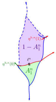
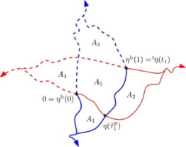
Figure 21. (a) The blue flow lines and dual flow lines from $\eta^{\mathrm{b},n}(0)$ (which happens to be a green edge here) and $\eta^{\mathrm{b},n}(1)$ (which happens to be a red edge), together with the red flow line from the tail of $\eta^{\mathrm{b}}(0)$. (b) The five-region picture in Proposition 5.18 in the case $t_{1}<0$. [Yiting: change $\eta^{\mathrm{r}}$ to ${}^{\mathrm{r}}\eta$ ]

Throughout this section we work in the setting of a usual coupling, where $\eta^{\mathrm{b}}$ is the zero-angle Peano curve in an imaginary geometry. Let $\eta^{\mathrm{r}}$ be the Peano curve of angle $\theta+\tfrac{\pi}{2}$ so that $\eta^{\theta}$ is a right boundary of $\eta^{\mathrm{r}}$. Let $\prescript{\mathrm{r}}{}{\eta}$ be the Peano curve of angle $\theta-\tfrac{\pi}{2}$, which is also the time reversal of $\eta^{\mathrm{r}}$. For $q\in\mathbb{Q}$, we define $t_{q}$ to be the a.s. unique time such that $\eta^{\mathrm{b}}(q)=\prescript{\mathrm{r}}{}{\eta}(t_{q})$. The time $t_{1}$ is negative if and only if $\eta^{\mathrm{b}}(1)$ is left of $\eta^{\theta}$, which is further equivalent to $\{\delta=1\}$ in Proposition 5.10. See Figure 21(b) for an illustration of this case. For concreteness we focus on this case in the rest of this section as the case $t_{1}>0$ can be treated in the same way. The left and right boundary of $\eta^{\mathrm{b}}$ at $t=0$ and $t=1$ and the left and right boundary of ${}^{r}\eta$ at $t=1$ and $t=t_{1}$ divide $\eta^{\mathrm{b}}([0,1])\cup\>\prescript{\mathrm{r}}{}{\eta}([t_{1},0])$ into five regions. We use $\{A_{i}\}_{1\leq i\leq 5}$ to denote the five regions as well as their $\mu_{\mathfrak{h}}$-area, as indicated in Figure 21(b). Note that $t_{1}=-A_{2}-A_{5}-A_{4}$ in this case.

We have a similar discrete picture for the sequence of UIWTs in a usual coupling. More precisely, let $\prescript{\mathrm{r}}{}{\mathfrak{y}}$ be the counterclockwise exploration path of a UIWT analogous to $\mathfrak{y}^{\mathrm{b}}$, and let $\prescript{\mathrm{r}}{}{Z}=(\prescript{\mathrm{r}}{}{R},\prescript{\mathrm{r}}{}{L})$ be the walk associated with $\prescript{\mathrm{r}}{}{\mathfrak{y}}$ (Section 2.2). For the $n$th UIWT in a usual coupling, let $\prescript{\mathrm{r}}{}{\mathfrak{y}}^{n}(t)=\prescript{\mathrm{r}}{}{\mathfrak{y}}(\lfloor 3nt\rfloor)$ and $\prescript{\mathrm{r}}{}{Z^{n}}=(\tfrac{1}{4n}\prescript{\mathrm{r}}{}{R}_{\lfloor 3nt\rfloor},\tfrac{1}{2n}\prescript{\mathrm{r}}{}{L}_{\lfloor 3nt\rfloor})$. (Note that the notation $\prescript{\mathrm{r}}{}{Z^{n}}$ has a different meaning from Section 2 and 3.) In light of Proposition 2.5 and the scaling in the definition of discrete quantum length, the abscissa and ordinate of $\prescript{\mathrm{r}}{}{Z^{n}}$ measure the net change of the discrete quantum length of the right and left “boundary” of $\prescript{\mathrm{r}}{}{\mathfrak{y}}^{n}$ respectively, which are dual red flow lines and red flow lines.

Let us define discrete analogues to $t_{q}$ via

$$t_{q}^{n}\colonequals\inf\{t\in\mathbb{R}\,:\,\mathfrak{y}^{\mathrm{b},n}(q)=\prescript{\mathrm{r}}{}{\mathfrak{y}}^{n}(t)\}\quad\forall\;q\in\mathbb{Q}.$$

In analogue with $(A_{i})_{1\leq i\leq 5}$, the region $\mathfrak{y}^{\mathrm{b},n}([0,1])\cup\prescript{\mathrm{r}}{}{\mathfrak{y}}^{n}([t^{n}_{1},0])$ can be divided into five subregions $(A^{n}_{i})_{1\leq i\leq 5}$ bounded by the red and blue flow lines and dual flow lines from $\mathfrak{y}^{\mathrm{b},n}(0)$ and $\mathfrak{y}^{\mathrm{b},n}(1)$. We also use the same notation $(A_{i}^{n})_{1\leq i\leq 5}$ to represent the discrete quantum areas ( Figure 22 (a)) of the corresponding subregion.

Remark 5.17.

When defining these five subregions and their discrete quantum areas, we are not careful about whether to include their boundaries or not. The reason is that these boundaries consist of portions of flow line and dual flow lines. Once scaled by $(3n)^{-1}$, they have $o(n^{-0.1})$ quantum area with superpolynomial probability. Therefore they are negligible in the scaling limit. This remark applies to all edge subsets whose discrete quantum areas are relevant. So we ignore the boundary issue from now on.

When we talk about the boundaries of these subregions, which are flow lines and dual flow lines, we simply say that they start from $\mathfrak{y}^{\mathrm{b},n}(0)$ and $\mathfrak{y}^{\mathrm{b},n}(1)$ without further specifying the starting vertex or face. The reason is that due to Remark 5.15, the precise starting point is immaterial in the scaling limit.

Since we assume $\delta=1$ in the continuum, in a usual coupling, $J^{n}_{1}-K^{n}_{1}$ in Proposition 5.10 converges to $1$ a.s. Therefore $\eta^{\mathrm{b},n}(1)$ is left of the red flow line from the tail of $\eta^{\mathrm{b},n}(0)$ for large enough $n$. See Figure 22 (a) for an illustration of the discrete picture in this case. Note that in this case $A^{n}_{1}$ in Proposition 5.14 is the same as $A^{n}_{1}$ defined here. Moreover, $A^{n}_{1}+A^{n}_{3}+A^{n}_{5}=1$.

Proposition 5.18.

In a usual coupling, $(A_{i}^{n})_{i=1}^{5}$ converges to $(A_{i})_{i=1}^{5}$ in probability.

Moreover, for any fixed $q\in\mathbb{Q}$, $t^{n}_{q}$ converges to $t_{q}$ in probability.

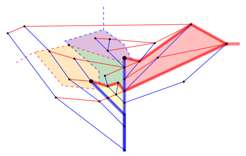
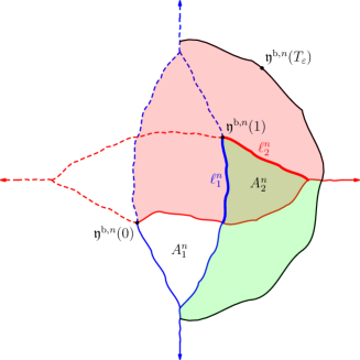
Figure 22. (a) The five regions in Figure 21 shown for a small portion of an infinite wooded triangulation. The tails of $\mathfrak{y}^{\mathrm{b},n}(0)$ and $\mathfrak{y}^{\mathrm{b},n}(1)$ are indicated with large dots, and flow lines from these vertices are shown in bold red and blue. Dual flow lines from $\mathfrak{y}^{\mathrm{b},n}(0)$ and $\mathfrak{y}^{\mathrm{b},n}(1)$ are shown as dashed. (b) To show that $A_{2}^{n}\to A_{2}$, we fix a large enough $T_{\varepsilon}>0$ and consider the region $\mathfrak{y}^{\mathrm{b},n}[0,T_{\varepsilon}]$. We define the green shaded area $B_{1}^{n}$ and the pink shaded area $B_{2}^{n}$ (the pink and green regions both include the region marked $A_{2}^{n}$) and note that the area of $\mathfrak{y}^{\mathrm{b},n}[0,T_{\varepsilon}]$ is equal to $A_{1}^{n}+B_{1}^{n}+B_{2}^{n}-A_{2}^{n}$. Thus $A_{2}^{n}=B_{1}^{n}+B_{2}^{n}-A_{1}^{n}-T_{\varepsilon}$.

Proof.

Suppose we are in the setting of a usual coupling; recall Proposition 5.14 and 5.16. We further assume that $t_{1}<0$ and $\delta=1$ as the other case is the same. Then Proposition 5.14 implies that $A_{1}^{n}\to A_{1}$ and $A^{n}_{3}+A^{n}_{5}\to A_{3}+A_{5}$ in probability. Regarding $\mathfrak{y}^{\mathrm{b},n}(1)$ as the root of the UIWT and considering the time reversal of $\mathfrak{y}^{\mathrm{b},n}$, we can treat $A^{3}_{n}$ as the right region of the dual red flow line. Since the bi-infinite word of a UIWT is stationary, the UIWT recentered at $\mathfrak{y}^{\mathrm{b},n}(1)$ is still a UIWT. Now the second statement (on $\overline{A}^{n}_{1}$) in Proposition 5.14 gives $A_{3}^{n}\to A_{3}$ in probability, hence $A_{5}^{n}\to A_{5}$ in probability.

Most of the remainder of the proof is dedicated to the convergence of $A_{2}^{n}$. We refer to Figure 22(b) for various quantities involved in this argument.

We first show that $(A_{2}^{n})_{n\in\mathbb{N}}$ are tight. By Proposition 5.10, the discrete quantum length $\ell^{n}_{1}$ of the blue flow line starting from $\mathfrak{y}^{\mathrm{b},n}(1)$ inside ${}^{r}\mathfrak{y}^{n}([t^{n}_{1},0])$ converges a.s. to a finite number. By the symmetry between blue and red in the UIWT, we can apply Proposition 5.10, 5.14 and 5.16 to the exploration ${}^{r}\mathfrak{y}^{n}$ for the UIWT recentered at $\mathfrak{y}^{\mathrm{b},n}(1)$. Then $A^{n}_{2}$ can be seen as the discrete quantum area of ${}^{r}\mathfrak{y}^{n}$ on the left of the blue flow line from $\mathfrak{y}^{\mathrm{b},n}(1)$, when the local time of this blue flow line reaches $(1+\sqrt{2}+o_{n}(1))\ell^{n}_{1}$ (recall Proposition 5.16). This gives the tightness of $A^{n}_{2}$.

Now we claim that for all $\varepsilon>0$, there exists $T_{\varepsilon}<\infty$ such that with probability $1-\varepsilon$, the regions $A^{n}_{1},A^{n}_{2},A^{n}_{3},A^{n}_{5}$ are all contained in $\mathfrak{y}^{\mathrm{b},n}[0,T_{\varepsilon}]$. To show this, note that we can recenter the UIWT at $\mathfrak{y}^{\mathrm{b},n}(1)$ and treat $\mathfrak{y}^{\mathrm{b},n}(0)$ as $\mathfrak{y}^{\mathrm{b},n}(-1)$. Therefore $A^{n}_{4}$ can be treated in the same way as $A^{n}_{2}$. In particular, $A^{n}_{4}$ is tight. Since we assume $\delta=1$, under a usual coupling, $J^{n}_{1}-K^{n}_{1}$ in Proposition 5.10 converges to $1$ a.s. Therefore

(5.4) $$t_{1}^{n}=-(A_{2}^{n}+A_{5}^{n}+A_{4}^{n})+o_{n}(1),$$

where $o_{n}(1)$ comes from Remark 5.17. This means $(t_{1}^{n})_{n\in\mathbb{N}}$ is tight. The same argument showing the tightness of $(A^{n}_{2})_{n\in\mathbb{N}}$ gives the existence of $T_{\varepsilon}$.

Now we work on the event $T_{\varepsilon}<\infty$. we define $B_{1}^{n}(T_{\varepsilon})$ to be the area of the intersection of $\mathfrak{y}^{\mathrm{b},n}([1,T_{\varepsilon}])$ and the region right of the red flow line from $\mathfrak{y}^{\mathrm{b},n}(1)$. We define $B_{2}^{n}(T_{\varepsilon})$ to be the area of the intersection of $\mathfrak{y}^{\mathrm{b},n}([0,T_{\varepsilon}])$ and the region left of the red flow line from $\mathfrak{y}^{\mathrm{b},n}(0)$. Then by the inclusion-exclusion principle applied to the discrete quantum area, we have

(5.5) $$A_{2}^{n}=B_{1}^{n}(T_{\varepsilon})+B_{2}^{n}(T_{\varepsilon})+A_{1}^{n}-T_{\varepsilon}.$$

The inclusion-exclusion principle also applies in the continuum, yielding a continuum analogue of (5.5) with the LHS being $A_{2}$ and the RHS being the continuum limit of the RHS of (5.5). This yields that $A_{2}^{n}\to A_{2}$ in probability.

As explained in the argument for the existence of $T_{\varepsilon}$, the region $A^{n}_{4}$ can be treated similarly as $A^{n}_{2}$ by recentering the UIWT at $\mathfrak{y}^{\mathrm{b},n}(1)$. Therefore $A_{4}^{n}\to A_{4}$ in probability. By (5.4), we have $t^{n}_{1}\to t_{1}$ in probability. The argument for general $t^{n}_{q}$ is the same. ∎

Proof of Theorem 5.1.

Suppose we are in a usual coupling. Since $\prescript{\mathrm{r}}{}{Z}^{n}$ converges in law, by possibly extracting a subsequence, we may further assume that in this coupling $\prescript{\mathrm{r}}{}{Z}^{n}$ converges to a Brownian motion $\mathscr{Z}=(\mathscr{R},\mathscr{L})$ a.s. in the locally uniform topology. We claim that

(5.6) $$\mathscr{L}=\widetilde{\mathscr{L}}\quad\textrm{and}\quad\mathscr{R}=\widetilde{\mathscr{R}}\quad\textrm{a.s.}$$

where $\widetilde{\mathscr{Z}}={\color[rgb]{0,0,0}(\widetilde{\mathscr{R}},\widetilde{\mathscr{L}})}$ is the Brownian motion associated with $(\mu_{\mathfrak{h}},$${}^{r}\eta)$ in Theorem 4.1. We postpone the proof of this claim and proceed to prove Theorem 5.1.

Let $\mathscr{Z}^{\mathrm{r}}$ denote the mating of tree Brownian motion associated with $(\mu_{\mathfrak{h}},$$\eta^{\mathrm{r}})$ and let $\mathscr{Z}^{\mathrm{g}}$ be the Brownian motion such that $(\mathscr{Z}^{\mathrm{b}},\mathscr{Z}^{\mathrm{r}})\overset{d}{=}(\mathscr{Z}^{\mathrm{r}},\mathscr{Z}^{\mathrm{g}})$. Note that in Theorem 5.1, the Brownian motions $\mathscr{Z}^{\mathrm{b}},\mathscr{Z}^{r},\mathscr{Z}^{\mathrm{g}}$ correspond to the Peano curves of angle $0,\tfrac{2\pi}{3},\tfrac{4\pi}{3}$ respectively. But at the moment we only know that $\eta^{\mathrm{b}}$ and $\eta^{\mathrm{r}}$ are of angle 0 and that $\theta+\tfrac{\pi}{2}$, respectively. We abuse notation with $\mathscr{Z}^{\mathrm{r}}$ and $\mathscr{Z}^{\mathrm{g}}$ here since we will see $\theta+\tfrac{\pi}{2}=\tfrac{2\pi}{3}$ momentarily. Note that $\mathscr{Z}^{\mathrm{b}},\mathscr{Z}^{\mathrm{r}},\mathscr{Z}^{\mathrm{g}}$ determine each other a.s.

Recall from Remark 5.2 that to simplify notation, we use $Z^{\mathrm{b},n},Z^{\mathrm{r},n},Z^{\mathrm{g},n}$ to denote the rescaled walks in Theorem 5.1. Proposition 3.7 and (5.6) imply that $(Z^{\mathrm{b},n},Z^{\mathrm{r},n})$ converges in law to $(\mathscr{Z}^{\mathrm{b}},\mathscr{Z}^{\mathrm{r}})$. As a result of the symmetry between colors, $(Z^{\mathrm{r},n},Z^{g,n})$ converges in law to $(\mathscr{Z}^{\mathrm{r}},\mathscr{Z}^{\mathrm{g}})$. Since $\mathscr{Z}^{\mathrm{b}},\mathscr{Z}^{\mathrm{r}},\mathscr{Z}^{\mathrm{g}}$ determine each other a.s., $(Z^{\mathrm{b},n},Z^{\mathrm{r},n},Z^{g,n})$ must jointly converge to $(\mathscr{Z}^{b},\mathscr{Z}^{r},\mathscr{Z}^{g})$. By symmetry $(\mathscr{Z}^{\mathrm{b}},\mathscr{Z}^{\mathrm{r}})\overset{d}{=}(\mathscr{Z}^{\mathrm{r}},\mathscr{Z}^{\mathrm{g}})\overset{d}{=}(\mathscr{Z}^{\mathrm{g}},\mathscr{Z}^{\mathrm{b}})$. This yields that the angle difference between $\eta^{\mathrm{b}}$ and $\eta^{\mathrm{r}}$ is $\tfrac{2\pi}{3}$ and $\theta=\tfrac{\pi}{6}$. This will conclude the proof of Theorem 5.1.

We are left to prove (5.6). We focus on proving $\mathscr{R}=\widetilde{\mathscr{R}}$ as $\mathscr{L}=\widetilde{\mathscr{L}}$ follows the same argument. By Proposition 5.18 and possibly extracting a subsequence, we can assume that in our coupling, $t_{q}^{n}\to t_{q}$ a.s. for all $q\in\mathbb{Q}$. By Proposition 2.12, 4.2 and 5.16, we have $\mathscr{R}_{t_{q}}=\tfrac{c}{1+\sqrt{2}}$ $\widetilde{\mathscr{R}}_{t_{q}}$ for all $q\in\mathbb{Q}$, where $c$ is the constant in Proposition 5.16. More precisely, for a fixed $q$, $\mathscr{R}_{t_{q}}$ and $\tfrac{c}{1+\sqrt{2}}$ $\widetilde{\mathscr{R}}_{t_{q}}$ are two expressions of the scaling limit of the relative change of discrete quantum length of the dual red flow line from time $0$ to time $t^{n}_{q}$. The $\mathscr{R}_{t_{q}}$ limit comes from the fact that $\prescript{\mathrm{r}}{}{Z}^{n}$ converges to $\mathscr{Z}=(\mathscr{R},\mathscr{L})$ a.s. locally uniformly. The $\tfrac{c}{1+\sqrt{2}}$ $\widetilde{\mathscr{R}}_{t_{q}}$ limit comes from the perspective where we view the lengths of the dual red flow lines as counting the local time of the left/right excursions for the counterclockwise exploration of the red tree. In particular, we apply Proposition 5.16 with $\mathcal{Z}$ and $\overline{Z}$ being the forward and reversed grouped-step walks of $\prescript{\mathrm{r}}{}{Z}^{n}$. Here we need to make sure that the merging time (w.r.t. the counterclockwise exploration of the red tree) of the dual red flow lines from $\mathfrak{y}^{\mathrm{b},n}(0)$ and $\mathfrak{y}^{\mathrm{b},n}(1)$ is tight as $n\to\infty$. To see this, let $e^{n}$ be the first common edge of these two dual flow red lines. Then the discrete quantum lengths from $e^{n}$ to $\mathfrak{y}^{\mathrm{b},n}(0)$ is tight due to the local uniform convergence of $\prescript{\mathrm{r}}{}{Z}^{n}$ and the tightness of $t_{q}^{n}$. This length can also be viewed as the local time accumulated for the left/right excursions for the counterclockwise exploration of the red tree until the merging time. Since the local time process converge to $(\ell^{p}_{t})_{t\geq 0}$ which goes to $\infty$ as $t\to\infty$, the merging time must be tight as desired.

Note that the set $\{\eta^{\mathrm{b}}(q)\}_{q\in\mathbb{Q}}$ is dense in $\mathbb{C}$. Therefore $\forall\;a<b$, the open set $\prescript{\mathrm{r}}{}{\eta}(a,b)$ contains a point in that set. This means that $\{t_{q}\,:\,q\in\mathbb{Q}\}$ is dense in $\mathbb{R}$. Since $\mathscr{R}_{t_{q}}=\tfrac{c}{1+\sqrt{2}}$ $\widetilde{\mathscr{R}}_{t_{q}}$ for all $q\in\mathbb{Q}$, we have that $\mathscr{R}_{t}=\tfrac{c}{1+\sqrt{2}}\widetilde{\mathscr{R}}_{t}$ a.s. for all $t\in\mathbb{R}$. Since $\mathscr{R}\overset{d}{=}\widetilde{\mathscr{R}}$ hence $c=1+\sqrt{2}$. This concludes the proof. ∎

Remark 5.19.

Our proof of Theorem 5.1 implies that when $\theta=\tfrac{\pi}{6}$ and $\kappa=16$, the constants $p$ and $c$ defined in Lemma 4.3 and Proposition 4.2 satisfy $p=\frac{\sqrt{2}}{1+\sqrt{2}}$ and $c=1+\sqrt{2}$. In [23], it is shown that $c=2$ when $\theta=\tfrac{\pi}{2}$ and $\kappa=12$. So far we don’t have a derivation for these values independent of discrete models. And we do not know the general dependence of $p$ and $c$ on $\theta$ and $\kappa$ except that $p(\tfrac{\pi}{2})=\frac{1}{2}$ holds for all $\kappa$ by symmetry.

5.4. From infinite- to finite-volume

We will prove Theorem 1.5 from Theorem 5.1 using a general approach for transferring convergence results of unconditioned random walks to the corresponding result for conditioned random walks. Roughly speaking, the idea is that a random walk conditioned on starting and ending at the origin and staying in the first quadrant is, away from the origin, sufficiently similar to the corresponding infinite-volume walk (see Proposition 5.20). A similar approach could be applied to the joint convergence result proved in [23].

Consider a Brownian motion $\mathscr{Z}$ distributed as $\mathscr{Z}^{\mathrm{b}}$ and denote by $\mathbb{P}$ the law of $\mathscr{Z}|_{[0,1]}$. For $\varepsilon\geq 0$, let $E^{\varepsilon}$ be the event that $\mathscr{Z}|_{[0,1]}\in[-\varepsilon,\infty)^{2}$ and $|\mathscr{Z}_{1}|\leq\varepsilon$, and define $\mathbb{P}^{\varepsilon}=\mathbb{P}[\cdot\,|\,E^{\varepsilon}]$. It is well known that $\mathbb{P}^{\varepsilon}$ converges weakly to $\mathbb{P}^{0}$ which is supported on the space of continuous curves in the first quadrant which start and end at the origin.

Let $\mathcal{Z}^{n}$ be the normalized lattice walk as defined at the beginning of Section 5.2, which has i.i.d. increments. Let $\mathbb{P}^{n}$ be the law of $\mathcal{Z}^{n}|_{[0,1]}$. For $\varepsilon>0$, let $E^{\varepsilon,n}$ be the event that $\mathcal{Z}^{n}|_{[0,1]}\in[-\varepsilon,\infty)^{2}$ and $|\mathcal{Z}^{n}_{1}|\leq\varepsilon$, and let $\mathbb{P}^{n,\varepsilon}=\mathbb{P}^{n}[\cdot\,|\,E^{\varepsilon,n}]$. Let $\mathbb{P}^{n,0}$ be the conditional law of $\mathcal{Z}^{n}|_{[0,1]}$ given that $\mathcal{Z}^{n}|_{[0,1]}$ remains in $\{(x,y)\in\mathbb{R}^{2}:x\geq 0;y\geq-\frac{1}{\sqrt{2n}}\}$ and starts and ends at the origin. Then $\mathbb{P}^{n,0}$ is the law of $\left(\tfrac{1}{\sqrt{4n}}\mathcal{L}_{\lfloor 2nt\rfloor}^{\mathrm{b},n},\tfrac{1}{\sqrt{2n}}\mathcal{R}_{\lfloor 2nt\rfloor}^{\mathrm{b},n}\right)$ in the proof of Proposition 3.8. In particular, $\mathbb{P}^{n,0}$ weakly converges to $\mathbb{P}^{0}$. The following proposition allows us to transfer weak convergence under $\mathbb{P}^{n}$ to the same result under $\mathbb{P}^{n,0}$.

Proposition 5.20.

Fix $0<\xi<u<1$. Let $\mathcal{F}_{\xi,u}$ be the sub-$\sigma$-algebra of the Borel $\sigma$-algebra of $\mathcal{C}([0,1],\mathbb{R}^{2})$ generated by the evaluation functionals at $x$, for all $x\in[\xi,u]$. Suppose $\{Y_{n}\}_{n\geq 1}$ and $Y$ are $\mathcal{F}_{\xi,u}$-measurable random variables. If the $\mathbb{P}^{n}$-law of $(\mathcal{Z}^{n},Y_{n})$ weakly converges to the $\mathbb{P}$-law of $(\mathscr{Z},Y)$, then the $\mathbb{P}^{n,0}$-law of $(\mathcal{Z}^{n},Y_{n})$ weakly converges to the $\mathbb{P}^{0}$-law of $(\mathscr{Z},Y)$.

We will prove Proposition 5.20 in Appendix A. Now we proceed to the proof of Theorem 1.5 and 1.6, which relies on Proposition 5.20 and several arguments similar to the ones in Sections 5.1–5.3. So we will only highlight the new technical ingredients.

We still use the same notations as in the infinite volume setting. Namely, let $S$ be a uniform wooded triangulation of size $n$ and $Z^{\mathrm{b}},Z^{\mathrm{r}},Z^{\mathrm{g}}$ be its encoding walks for counterclockwise explorations. Let $\mathcal{Z}=(\mathcal{L},\mathcal{R})$ be the grouped-step walk of $\mathcal{Z}^{\mathrm{b}}$ as defined in Lemma 3.1. Let $Z^{\mathrm{b},n},Z^{\mathrm{r},n},Z^{\mathrm{g},n}$ be the rescaled walks in Theorem 1.5 and $\mathcal{Z}^{n}=(\tfrac{1}{\sqrt{4n}}\mathcal{L}^{n}_{2nt},\tfrac{1}{\sqrt{2n}}\mathcal{R}^{n}_{2nt})$.

Remark 5.21 (Abuse of notations in the finite-volume setting).

In Section 3 we used $S^{n}$ to denote a uniform wooded triangulation of size $n$, $Z^{\mathrm{b},n},Z^{\mathrm{r},n},Z^{\mathrm{g},n}$ to denote the corresponding unscaled random walks, and $\mathcal{Z}^{\mathrm{b},n}$ as the grouped-step walk of $Z^{\mathrm{b},n}$. In this section we denote them by $S$, $Z^{\mathrm{b}}$, $Z^{\mathrm{r}}$, $Z^{\mathrm{g}}$, and $\mathcal{Z}$ for simplicity. On the other hand, we use $Z^{\mathrm{b},n},Z^{\mathrm{r},n},Z^{\mathrm{g},n}$ and $\mathcal{Z}^{n}$ to denote the rescaled walks as in the infinite volume case; see Remark 5.2. Similarly, most of our notations below are in parallel to the infinite volume case. This is convenient because our finite-volume result is derived from the infinite volume case.

By Lemma 3.1, the law of $\mathcal{Z}^{n}$ is $\mathbb{P}^{n,0}$ above.

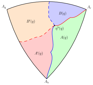
Figure 23. The red and blue flow lines and dual flow lines from $\eta^{\mathrm{b}}(q)$ divide the unit area $1$-LQG sphere into four regions whose areas are $A(q)$, $B(q)$, $A^{\prime}(q)$, $B^{\prime}(q)$ as indicated. In the continuum, the outer face $\Delta A_{\mathrm{b}}A_{\mathrm{r}}A_{\mathrm{g}}$ should be viewed as $\infty$.

For $q\in(0,1)\cap\mathbb{Q}$, we can define left and right excursion for $\mathcal{Z}^{n}|_{[q,1]}-\mathcal{Z}^{n}_{q}$ as in Section 5.1 and 5.2. Let $\mathcal{A}^{n}(q)$ and $\mathcal{B}^{n}(q)$ be the total time in the right and left excursions during $[q,1]$ respectively. In the continuum, let $\mu_{\mathfrak{h}},\eta^{\mathrm{b}},\eta^{\mathrm{r}},\eta^{\mathrm{g}}$ and $\mathscr{Z}^{\mathrm{b}},\mathscr{Z}^{\mathrm{r}},\mathscr{Z}^{\mathrm{g}}$ be defined as in Theorem 1.5. Note that $\mu_{\mathfrak{h}}$ has unit mass. Let $\eta^{\theta}_{q}$ be the flow line from $\eta^{\mathrm{b}}(q)$ of angle $\theta\colonequals\tfrac{\pi}{6}$. Let $A(q)$ and $B(q)$ be the $\mu_{\mathfrak{h}}$-area in $\eta^{\mathrm{b}}[q,1]$ on the right and left of $\eta^{\theta}_{q}$ (see Figure 23). We claim that

(5.7) $$(\mathcal{Z}^{n},\mathcal{A}^{n}(q),\mathcal{B}^{n}(q))\to(\mathscr{Z}^{\mathrm{b}},A(q),B(q))\quad\textrm{in law}.$$

For $\varepsilon>0$ small, let $\mathcal{A}^{n,\varepsilon}(q)$ and $\mathcal{B}^{n,\varepsilon}(q)$ be the total time in the right and left excursions during $[q,1-\varepsilon]$ respectively. And let $A^{\varepsilon}(q)$ and $B^{\varepsilon}(q)$ be the $\mu_{\mathfrak{h}}$-area in $\eta^{\mathrm{b}}[q,1-\varepsilon]$ on the right and left of $\eta^{\theta}_{q}$. The by Proposition 5.10 and 5.20, $(\mathcal{Z}^{n},\mathcal{A}^{\varepsilon}(q),\mathcal{B}^{\varepsilon}(q))\to(\mathscr{Z}^{\mathrm{b}},A^{\varepsilon}(q),B^{\varepsilon}(q))$ in law. By the tightness of $(\mathcal{Z}^{n},\mathcal{A}^{n}(q),\mathcal{B}^{n}(q))$, by possibly extracting a subsequence, we may find a coupling so that a.s. $(\mathcal{A}^{n}(q),\mathcal{B}^{n}(q))$ converges to some $(A,B)$ and $(\mathcal{A}^{n,\varepsilon}(q),\mathcal{B}^{n,\varepsilon}(q))\to(A^{\varepsilon}(q),B^{\varepsilon}(q))$ for all rational $\varepsilon$. Since $\mathcal{A}^{n,\varepsilon}(q)\leq\mathcal{A}^{n}(q)$ and $\mathcal{B}^{n,\varepsilon}(q)\leq\mathcal{B}^{n}(q)$, we have $A^{\varepsilon}(q)\leq A$ and $B^{\varepsilon}\leq B$ a.s. Letting $\varepsilon\to 0$, we have $A(q)\leq A$ and $B(q)\leq B$ a.s. On the other hand, $A+B=A(q)+B(q)=1-q$. Therefore $A(q)=A$ and $B(q)=B$ a.s. This proves (5.7).

Let $\mathfrak{y}^{\mathrm{b},n}$ be the rescaled clockwise blue tree exploration path of the Schnyder wood as in the infinite volume setting. Let $A^{n}(q)$ and $B^{n}(q)$ be the discrete quantum area of $\eta^{\mathrm{b}}[q,1]$ on the right and left of the red flow line from $\mathfrak{y}^{\mathrm{b},n}(q)$. We claim that due to (5.7) we have $(Z^{\mathrm{b},n},A^{n}(q),B^{n}(q))\to(\mathscr{Z}^{\mathrm{b}},A(q),B(q))$ in law. There are two caveats for this claim: (1) the time $q$ for $\eta^{\mathrm{b},n}$ (i.e., for $Z^{\mathrm{b},n}$) is not exactly the same as the time $q$ for $\mathcal{Z}$; (2) the boundary contributions of the two regions $A^{n}(q)$ and $B^{q}(n)$ are nonzero. These two concerns are handled by Remark 5.15 and 5.17, respectively. Note that the $o_{n}(1)$ errors there have rapidly decaying tails, in the contrast to the polynomial decay of the conditioning event in Proposition 2.6. Therefore the two remarks also apply to the finite volume setting, and the claim holds.

For $q\in(0,1)$, we can reverse $\mathfrak{y}^{\mathrm{b},n}$ to define the left and right excursions of the dual red flow line from time $q$ to time $0$. Let $A^{\prime n}(q),B^{\prime n}(q)$ be the discrete quantum area of on the left and right of that dual flow line and $A^{\prime}(q),B^{\prime}(q)$ be their continuum analog (see Figure 23). Then similar to the forward case, we have $(Z^{\mathrm{b},n},A^{\prime n}(q),B^{\prime n}(q))\to(\mathscr{Z}^{\mathrm{b}},A^{\prime}(q),B^{\prime}(q))$ in law. Let $\mathfrak{y}^{\mathrm{r},n}$ be the clockwise red tree exploration and $t^{n}_{q}=:\inf\{t:\mathfrak{y}^{\mathrm{r},n}(t)=\mathfrak{y}^{\mathrm{b},n}(q)\}$. Then $t^{n}_{q}=A^{n}(q)+A^{\prime n}(q)+o_{n}(1)$ where $o_{n}(1)$ comes from Remark 5.17. Let $t_{q}$ be the a.s. unique time such that $\eta^{\mathrm{b}}(q)=\eta^{\mathrm{r}}(t_{q})$. Then

(5.8) $$(Z^{\mathrm{b},n},t^{n}_{q})\to(\mathscr{Z}^{\mathrm{b}},t_{q})\quad\textrm{in law}\quad\forall\;q\in(0,1)\cap\mathbb{Q}.$$

Consider a coupling such that $Z^{\mathrm{b},n}\to\mathscr{Z}^{\mathrm{b}}$ and $t^{n}_{q}\to t_{q}$ a.s. for all $q\in(0,1)\cap\mathbb{Q}$. Let $\mathfrak{l}^{n}(q)$ be the local time accumulated by $\mathcal{Z}^{n}|_{[q,1]}-\mathcal{Z}^{n}_{q}$ during $[q,1]$ defined as in (5.1). By possibly extracting a subsequence, we may further assume $Z^{\mathrm{r},n}$ converges a.s. to some $\mathscr{Z}=(\mathscr{L},\mathscr{R})$ and $\lim_{n\to\infty}\mathfrak{l}^{n}(q)$ exists a.s. Write $Z^{\mathrm{r},n}=(L^{\mathrm{r},n},R^{\mathrm{r},n})$. By Proposition 2.1, $R^{\mathrm{r},n}_{t^{n}_{q}}$ is the total discrete quantum length of the red flow from $\mathfrak{y}^{\mathrm{b},n}(q)$. By a truncation argument similar to the one used above to show $A(q)\leq A$, combined with Proposition 4.2, we have

(5.9) $$\lim_{n\to\infty}\mathfrak{l}^{n}(q)\leq(1+\sqrt{2})\mathscr{R}_{t_{q}}.$$

Write $\mathscr{Z}^{\mathrm{r}}$ in Theorem 1.5 as $(\mathscr{L}^{\mathrm{r}},\mathscr{R}^{\mathrm{r}})$. Then the quantum length of $\eta^{\theta}\cap\eta^{\mathrm{b}}[q,1]$ equals $\mathscr{R}^{r}_{t_{q}}$. Remark 3.6 and (3.2) in Lemma 3.5 ensures that Lemma 5.16 can be applied to the finite volume setting. Combined with (5.9), we have $\mathscr{R}^{\mathrm{r}}_{t_{q}}\leq\mathscr{R}_{t_{q}}$.

Since $\{t_{q}\}_{q\in(0,1)\cap\mathbb{Q}}$ is dense in $[0,1]$ as in the proof of Theorem 5.1, $\mathscr{R}^{\mathrm{r}}_{t}\leq\mathscr{R}_{t}$ a.s. for all $t\in[0,1]$. Since $\mathscr{R}\overset{d}{=}\mathscr{R}^{r}$, we must have $\mathscr{R}=\mathscr{R}^{\mathrm{r}}$ a.s. The same argument gives $\mathscr{L}=\mathscr{L}^{\mathrm{r}}$. Thus $(Z^{\mathrm{b},n},Z^{\mathrm{r},n})$ converge to $(\mathscr{Z}^{\mathrm{b}},\mathscr{Z}^{r})$ in law. By symmetry in the role of the colors, we conclude the proof of Theorem 1.5.

To prove Theorem 1.6, note that $(Z^{\mathrm{b},n},A^{n}(t))\to(\mathscr{Z}^{\mathrm{b}},A(t))$ in law for all $t\in[0,1]$. Therefore the discrete quantum area of the region bounded by red and blue flow lines from a uniformly chosen vertex converges to the corresponding continuum quantum area. The ratio between the number of faces and edges in this region is $2:3$, modulo the negligible boundary contribution (Remark 5.17). This gives the convergence of the $z$-coordinate (Figure 4.) in Theorem 1.6. Since $(Z^{\mathrm{b},n},Z^{\mathrm{r},n},Z^{\mathrm{g},n})$ jointly converge as in Theorem 1.5, the three coordinates jointly converge as stated in Theorem 1.6.

Appendix A Proof of Proposition 5.20

Suppose we are in the setting of Proposition 5.20. For a probability measure $\mathbb{Q}$ on $\mathcal{C}([0,1],\mathbb{R}^{2})$ under the uniform topology, let $\mathbb{Q}_{\xi,u}$ be $\mathbb{Q}$ restricted to $\mathcal{F}_{\xi,u}$. Since $\mathcal{Z}^{n}_{1}$ under $\mathbb{P}^{n}$ converges to $\mathscr{Z}_{1}$ under $\mathbb{P}$, we have that $Y_{n}$ under $\mathbb{P}^{n,\varepsilon}$ weakly converges to $Y$ under $\mathbb{P}^{\varepsilon}$. Therefore, Proposition 5.20 follows from Lemma A.1 and A.2 below.

Lemma A.1.

(A.1) $$d_{\mathrm{tv}}(\mathbb{P}^{\varepsilon}_{\xi,u},\mathbb{P}^{0}_{\xi,u})=o_{\varepsilon}(1),$$

where $d_{\mathrm{tv}}$ denotes the total variational distance.

Lemma A.2.

(A.2) $$d_{\mathrm{tv}}(\mathbb{P}^{n,\varepsilon}_{\xi,u},\mathbb{P}^{n,0}_{\xi,u})=o_{\varepsilon}(1),$$

where $o_{\varepsilon}(1)$ is uniform in $n$.

Proof of Lemma A.1.

Denote by $\mathscr{Z}^{\varepsilon}$ a sample from $\mathbb{P}^{\varepsilon}$, for all $\varepsilon\geq 0$. We want to find a coupling $\mathbb{Q}^{\varepsilon}$ of $\mathscr{Z}^{\varepsilon}$ and $\mathscr{Z}^{0}$ such that

(A.3) $$\mathbb{Q}^{\varepsilon}[\mathscr{Z}^{\varepsilon}_{t}=\mathscr{Z}^{0}_{t}\;\;\textrm{for all}\;\xi\leq t\leq u]=1-o_{\varepsilon}(1).$$

Let $\xi_{0}=\xi/2$ and $u_{0}=(u+1)/2$. Let $G^{\varepsilon}=\{\mathscr{Z}^{\varepsilon}|_{[\xi_{0},u_{0}]}\in[-\varepsilon,\infty)^{2}\}$ for all $\varepsilon\geq 0$. Let $\widetilde{\mathscr{Z}}^{\varepsilon}$ and $\widetilde{\mathscr{Z}}^{0}$ be $\mathscr{Z}$ conditioned on $E^{\varepsilon}\setminus G^{\varepsilon}$ and $E^{0}\setminus G^{0}$ respectively. We start by showing that there exists a coupling $\widetilde{\mathbb{Q}}^{\varepsilon}$ of $\widetilde{\mathscr{Z}}^{\varepsilon}$ and $\widetilde{\mathscr{Z}}^{0}$ where

(A.4) $$\widetilde{\mathbb{Q}}^{\varepsilon}[\widetilde{\mathscr{Z}}^{\varepsilon}_{t}=\widetilde{\mathscr{Z}}^{0}_{t}\;\;\textrm{for all}\;\xi\leq t\leq u]=1-o_{\varepsilon}(1).$$

We first notice that

(A.5) $$\lim_{\varepsilon\to 0}(\widetilde{\mathscr{Z}}^{\varepsilon}_{\xi_{0}},\widetilde{\mathscr{Z}}^{\varepsilon}_{u_{0}})=(\widetilde{\mathscr{Z}}^{0}_{\xi_{0}},\widetilde{\mathscr{Z}}^{0}_{u_{0}})\quad\textrm{in law}.$$

By Skorohod’s embedding theorem, we can find a coupling $\widetilde{\mathbb{Q}}$ of $\{\widetilde{\mathscr{Z}}^{\varepsilon}\}_{\varepsilon\geq 0}$ such that for each fixed $\delta_{0}>0$,

$$\widetilde{\mathbb{Q}}[|\widetilde{\mathscr{Z}}^{\varepsilon}_{\xi_{0}}-\widetilde{\mathscr{Z}}^{0}_{\xi_{0}}|>\delta_{0}]=o_{\varepsilon}(1)\quad\textrm{and}\quad\widetilde{\mathbb{Q}}[|\widetilde{\mathscr{Z}}^{\varepsilon}_{u_{0}}-\widetilde{\mathscr{Z}}^{0}_{u_{0}}|>\delta_{0}]=o_{\varepsilon}(1)$$

where $o_{\varepsilon}(1)$ depends only on $\delta_{0},\xi,$ and $u$. For all $\varepsilon>0$, given a sample of $(\widetilde{\mathscr{Z}}^{\varepsilon},\widetilde{\mathscr{Z}}^{0})$ under $\widetilde{\mathbb{Q}}$, we claim that by resampling $\widetilde{\mathscr{Z}}^{\varepsilon}|_{[\xi_{0},u_{0}]}$ and $\widetilde{\mathscr{Z}}^{0}|_{[\xi_{0},u_{0}]}$ conditioned on $\widetilde{\mathscr{Z}}^{\varepsilon}_{[0,\xi_{0}]},$ $\widetilde{\mathscr{Z}}^{\varepsilon}_{[u_{0},1]},$ $\widetilde{\mathscr{Z}}^{0}_{[0,\xi_{0}]},$ $\widetilde{\mathscr{Z}}^{0}_{[u_{0},1]}$, we can obtain a coupling satisfying (A.4).

In fact, the $[\xi_{0},u_{0}]$ segment of $\widetilde{\mathscr{Z}}^{\varepsilon}$ and $\widetilde{\mathscr{Z}}^{0}$ are both planar Brownian bridges conditioning on its end points. Therefore, by the explicit Brownian heat kernel, we can couple $(\widetilde{\mathscr{Z}}^{\varepsilon},\widetilde{\mathscr{Z}}^{0})$ so that

(A.6) $$\widetilde{\mathbb{Q}}^{\varepsilon}\left[\widetilde{\mathscr{Z}}^{\varepsilon}_{\xi_{0}}=\widetilde{\mathscr{Z}}^{0}_{\xi_{0}}\;\;\textrm{and}\;\widetilde{\mathscr{Z}}^{\varepsilon}_{u_{0}}=\widetilde{\mathscr{Z}}^{0}_{u_{0}}\right]=1-o_{\varepsilon}(1).$$

Now we can resample the $[\xi_{0},u_{0}]$ segment of $\widetilde{\mathscr{Z}}^{\varepsilon}$ and $\widetilde{\mathscr{Z}}^{0}$ using the same Brownian bridge to achieve (A.4).

For all $\varepsilon\geq 0$, the process $\mathscr{Z}^{\varepsilon}$ is $\widetilde{\mathscr{Z}}^{\varepsilon}$ conditioning on $G^{\varepsilon}$. Since $\widetilde{\mathbb{Q}}^{\varepsilon}[G^{\varepsilon}\Delta G^{0}]=o_{\varepsilon}(1)$ and $\widetilde{\mathbb{Q}}^{\varepsilon}[G^{0}]\asymp 1$, by a further rejection sampling, we can find a coupling $\mathbb{Q}^{\varepsilon}$ satisfying (A.3). ∎

Proof of Lemma A.2.

The proof goes exactly in the same way as Lemma A.1. So we only point out the necessary modification. Recall the setting of Lemma A.1. We use the notations $\mathcal{Z}^{n,\varepsilon}$, $\mathcal{Z}^{n,0}$, $G^{n,\varepsilon}$, $G^{n,0}$, $\mathbb{Q}^{n,\varepsilon}$, $\widetilde{\mathbb{Q}}^{n,\varepsilon}$, $\widetilde{\mathbb{Q}}^{n}$, $\widetilde{\mathcal{Z}}^{n,\varepsilon}$, $\widetilde{\mathcal{Z}}^{n,0}$ to denote the discrete analogues of $\mathscr{Z}^{\varepsilon},\mathscr{Z}^{0},G^{\varepsilon},G^{0},\mathbb{Q}^{\varepsilon},\widetilde{\mathbb{Q}}^{\varepsilon},\widetilde{\mathbb{Q}},\widetilde{\mathscr{Z}}^{\varepsilon},\widetilde{\mathscr{Z}}^{0}$.

We can first find a coupling $\widetilde{\mathbb{Q}}^{n}$ of $\widetilde{\mathcal{Z}}^{n,\varepsilon}$ and $\widetilde{\mathcal{Z}}^{n,0}$ such that for each fixed $\delta_{0}>0$

$$\mathbb{Q}^{n}\left[|\mathcal{Z}^{n,\varepsilon}_{\xi_{0}}-\mathcal{Z}^{n,0}_{\xi_{0}}|>\delta_{0}\right]=o_{\varepsilon}(1)\quad\textrm{and}\quad\mathbb{Q}^{n}\left[|\mathcal{Z}^{n,\varepsilon}_{u_{0}}-\mathcal{Z}^{n,0}_{u_{0}}|>\delta_{0}\right]=o_{\varepsilon}(1)$$

where the quantity denoted $o_{\varepsilon}(1)$ may depend on $\delta_{0},\xi,u$, but not on $n$. In fact, by the invariance principle of random walk in cones [17],

(A.7) $$\lim_{n\to\infty}(\widetilde{\mathcal{Z}}^{n,\varepsilon}_{\xi_{0}},\widetilde{\mathcal{Z}}^{n,\varepsilon}_{u_{0}})=(\widetilde{Z}^{\varepsilon}_{\xi_{0}},\widetilde{Z}^{\varepsilon}_{u_{0}})\;\;\textrm{and}\;\;\lim_{n\to\infty}(\widetilde{\mathcal{Z}}^{n,0}_{\xi_{0}},\widetilde{\mathcal{Z}}^{n,0}_{u_{0}})=(\widetilde{Z}^{0}_{\xi_{0}},\widetilde{Z}^{0}_{u_{0}})\;\;\textrm{in law}.$$

Now the existence of $\widetilde{\mathbb{Q}}^{n}$ is equivalent to the definition of weak convergence in terms of Lévy-Prokhorov metric.

We can perform a resampling procedure analogous to the one in Lemma A.1 to get $\widetilde{\mathbb{Q}}^{n,\varepsilon}$ such that

(A.8) $$\widetilde{\mathbb{Q}}^{n,\varepsilon}\left[\widetilde{\mathcal{Z}}^{n,\varepsilon}_{t}=\widetilde{\mathcal{Z}}^{n,0}_{t}\;\;\textrm{for all}\;\xi\leq t\leq u\right]=1-o_{\varepsilon}(1).$$

The only difference is that the $[\xi_{0},u_{0}]$ segment of $\widetilde{\mathcal{Z}}^{\varepsilon}$ and $\widetilde{\mathcal{Z}}^{0}$ are planar random walk bridges rather than Brownian bridges. Therefore we need to use a random walk heat kernel estimate (in place of the Brownian motion heat kernel) to couple $(\widetilde{\mathcal{Z}}^{n,\varepsilon},\widetilde{\mathcal{Z}}^{n,0})$ so that

(A.9) $$\widetilde{\mathbb{Q}}^{n,\varepsilon}[\widetilde{\mathcal{Z}}^{n,\varepsilon}_{\xi_{0}}=\widetilde{\mathcal{Z}}^{n,0}_{\xi_{0}}\;\;\textrm{and}\;\widetilde{\mathcal{Z}}^{n,\varepsilon}_{u_{0}}=\widetilde{\mathcal{Z}}^{n,0}_{u_{0}}]=1-o_{\varepsilon}(1).$$

Since the increment $\xi$ of our walk in Lemma 3.1 satisfies $E[e^{b|\xi|}]<\infty$ for some $b>0$ and has zero mean, the following local central limit theorem (as an immediate corollary of [40, Theorem 2.3.11]) can be applied to find the coupling in (A.9):

Let $p_{n}$ be the heat kernel of the random walk $\mathbb{P}^{\infty}$ in Lemma 3.1 and $\bar{p}_{n}$ be the heat kernel of the Brownian motion. When we estimate $p_{n}$ using CLT, then

(A.10) $$(p_{n}(x)+p_{n+1}(x))/2=\bar{p}_{n}(x)\exp\left\{O\left(\frac{1}{\sqrt{n}}\right)+O\left(\frac{|x|}{n}\right)\right\},\;\;\quad\forall\;|x|\leq\sqrt{n}\log n.$$

The appearance of $(p_{n}(x)+p_{n+1}(x))/2$ is due to the parity issue, namely that $p_{n}(0,0)=0$ for odd $n$. However, (A.10) implies the desired result in our case, since $\widetilde{\mathcal{Z}}^{n,\varepsilon}_{\xi_{0}}$ and $\widetilde{\mathcal{Z}}^{n,0}_{\xi_{0}}$ (as well as $\widetilde{\mathcal{Z}}^{n,\varepsilon}_{u_{0}}$ and $\widetilde{\mathcal{Z}}^{n,0}_{u_{0}}$) are always in the same parity class, as they are two possible locations of a random walk at the same time.

The rest of the argument is the same as in the proof of Lemma A.1. ∎

Remark A.3.

Our proof of Proposition 5.20 holds for all lattice walks with zero mean and some finite exponential moment. This is useful when one studies the scaling limit of the mating of trees encoding of other decorated random planar maps, such as the spanning-tree-decorated maps and bipolar oriented maps [62, 37]. Moreover, in light of [40, Lemma 2.4.3], we expect that the finite exponential moment assumption can be significantly weakened. However, we won’t pursue this here.

Typesetting note. The figures in this article were produced using Asymptote, SageMath, TikZ, and Ipe.

Acknowledgment: We thank Olivier Bernardi, Ewain Gwynne, Nina Holden, Richard Kenyon and Scott Sheffield for helpful discussions. We are also grateful to the anonymous referees for their thorough and helpful feedback on an early version of the paper.

References

- [1] Juhan Aru, Yichao Huang and Xin Sun, Two perspectives of the 2D unit area quantum sphere and their equivalence, Comm. Math. Phys. 356 (2017), no. 1, 261–283, DOI 10.1007/s00220-017-2979-6. MR 3694028
- [2] Rodney Baxter, F model on a triangular lattice, J. Math. Phys. 10 (1969), no. 7, 1211–1216, DOI 10.1063/1.1664960.
- [3] Itai Benjamini and Oded Schramm, Recurrence of distributional limits of finite planar graphs, Electron. J. Probab. 6 (2001), no. 23, 1–13, DOI 10.1214/EJP.v6-96. MR 2883381
- [4] NathanaÎl Berestycki and Ellen Powell, Gaussian free field, Liouville quantum gravity and Gaussian multiplicative chaos, Lecture notes, 2021. available at this website.
- [5] Olivier Bernardi, Bijective counting of tree-rooted maps and shuffles of parenthesis systems, Electron. J. Combin. 14 (2007), no. 9, 1–36, DOI 10.37236/928. MR 2285813
- [6] Olivier Bernardi and Nicolas Bonichon, Intervals in Catalan lattices and realizers of triangulations, J. Combin. Theory Ser. A 116 (2009), no. 1, 55–75, DOI 10.1016/j.jcta.2008.05.005. MR 2469248
- [7] Olivier Bernardi and Éric Fusy, Schnyder decompositions for regular plane graphs and application to drawing, Algorithmica, 62 (2012), no. 3–4 1159–1197, DOI 10.1007/s00453-011-9514-5. MR 2871142
- [8] Olivier Bernardi, Nina Holden and Xin Sun, Percolation on triangulations: A bijective path to Liouville quantum gravity, Mem. Amer. Math. Soc., to appear.
- [9] Dmitry Chelkak, Hugo Duminil-Copin, Clément Hongler, Antti Kemppainen and Stanislav Smirnov, Convergence of Ising interfaces to Schramm’s SLE curves, C. R. Acad. Sci. Paris, Ser. I 352 (2014), no. 2, 157–161, DOI 10.1016/j.crma.2013.12.002. MR 3151886
- [10] François David, Antti Kupiainen, Rémi Rhodes and Vincent Vargas, Liouville quantum gravity on the Riemann sphere, Comm. Math. Phys. 342 (2016), no. 3, 869–907, DOI 10.1007/s00220-016-2572-4. MR 3465434
- [11] Giuseppe Di Battista and Fabrizio Frati, Drawing trees, outerplanar graphs, series-parallel graphs, and planar graphs in a small area, Thirty essays on geometric graph theory, Springer, New York, 2013, pp. 121–165. MR 3205153
- [12] Jian Ding, Julien Dubédat, Alexander Dunlap and Hugo Falconet, Tightness of Liouville first passage percolation for , Publ. Math. Inst. Hautes Études Sci. 132 (2020), no. 1, 353–403, DOI 10.1007/s10240-020-00121-1. MR 4179836
- [13] Monroe D. Donsker and S. R. S. Varadhan, Asymptotic evaluation of certain Markov process expectations for large time, I, Comm. Pure Appl. Math. 28 (1975), no 1, 1–47, DOI 10.1002/cpa.3160280102. MR 0386024
- [14] Monroe D. Donsker and S. R. S. Varadhan, Asymptotic evaluation of certain Markov process expectations for large time, II, Comm. Pure Appl. Math. 28 (1975), no. 2, 279–301, DOI 10.1002/cpa.3160280206. MR 0386024
- [15] Bertrand Duplantier, Jason Miller and Scott Sheffield, Liouville quantum gravity as a mating of trees, Asterisque, to appear.
- [16] Bertrand Duplantier and Scott Sheffield, Liouville quantum gravity and KPZ, Invent. Math. 185 (2011), no. 2, 333–393, DOI 10.1007/s00222-010-0308-1. MR 2819163
- [17] Jetlir Duraj and Vitali Wachtel, Invariance principles for random walks in cones, Stochastic Process. Appl. 130 (2020), no.7, 3920–-3942, DOI 10.1016/j.spa.2019.11.004. MR 4102254
- [18] István Fáry, On straight line representation of planar graphs, Acta Univ. Szeged. Sect. Sci. Math. 11 (1948), no. 4, 229–233. MR 0026311
- [19] Stefan Felsner, Éric Fusy, Marc Noy and David Orden, Bijections for Baxter families and related objects, J. Combin. Theory Ser. A 118 (2011), no. 3, 993–1020, DOI 10.1016/j.jcta.2010.03.017. MR 2763051
- [20] Stefan Felsner and Florian Zickfeld, Schnyder woods and orthogonal surfaces, Discrete Comput. Geom. 40 (2008), no. 1, 103–126, DOI 10.1007/s00454-007-9027-9. MR 2429650
- [21] Hubert de Fraysseix, János Pach and Richard Pollack, How to draw a planar graph on a grid, Combinatorica 10 (1990), no. 1, 41–51, DOI 10.1007/BF02122694. MR 1075065
- [22] Ewain Gwynne, Nina Holden, Jason Miller and Xin Sun, Brownian motion correlation in the peanosphere for , Ann. Inst. Henri Poincaré Probab. Stat. 53 (2017), no. 4, 1866–1889, DOI 10.1214/16-AIHP774. MR 3729638
- [23] Ewain Gwynne, Nina Holden and Xin Sun, Joint scaling limit of a bipolar-oriented triangulation and its dual in the peanosphere sense, arXiv:1603.01194.
- [24] Ewain Gwynne, Nina Holden and Xin Sun, Mating of trees for random planar maps and Liouville quantum gravity: a survey , Panoramas et Synthèses, to appear.
- [25] Ewain Gwynne, Nina Holden and Xin Sun, A mating-of-trees approach for graph distances in random planar maps, Probab. Theory Related Fields 177 (2020), no. 3–4, 1043–1102, DOI 10.1007/s00440-020-00969-8. MR 4126936
- [26] Ewain Gwynne, Adrien Kassel, Jason Miller and David B. Wilson, Active spanning trees with bending energy on planar maps and SLE-decorated Liouville quantum gravity for , Comm. Math. Phys. 358 (2018), no. 3, 1065–-1115, DOI 10.1007/s00220-018-3104-1. MR 3778352
- [27] Ewain Gwynne, Cheng Mao and Xin Sun, Scaling limits for the critical Fortuin-Kasteleyn model on a random planar map I: cone times, Ann. Inst. Henri Poincaré Probab. Stat. 55 (2019), no. 1, 1–60, DOI 10.1214/17-AIHP874. MR 3901640
- [28] Ewain Gwynne and Jason Miller, Existence and uniqueness of the Liouville quantum gravity metric for , Invent. Math. 223 (2021), no. 1, 213–333, DOI 10.1007/s00222-020-00991-6. MR 4199443
- [29] Ewain Gwynne, Jason Miller and Scott Sheffield. The Tutte embedding of the Poisson-Voronoi tessellation of the Brownian disk converges to -Liouville quantum gravity, Comm. Math. Phys. 374 (2020), no. 2, 735–784, DOI 10.1007/s00220-019-03610-5. MR 4072229
- [30] Ewain Gwynne, Jason Miller, and Scott Sheffield, The Tutte embedding of the the mated-CRT map converges Liouville quantum gravity, Ann. Probab. 49 (2021), no. 4, 1677–1717 DOI 10.1214/20-AOP1487. MR 4260465
- [31] Ewain Gwynne, Jason Miller, and Scott Sheffield, An invariance principle for ergodic scale-free random environments, Acta Math. 228 (2022), no. 2, 303–384, DOI: 10.4310/ACTA.2022.v228.n2.a2. MR 4448682
- [32] Ewain Gwynne and Xin Sun, Scaling limits for the critical Fortuin-Kasteleyn model on a random planar map II: local estimates and empty reduced word exponent, Electron. J. Probab. 22 (2017), no. 45, 1–56, DOI 10.1214/17-EJP64. MR 3661659
- [33] Ewain Gwynne and Xin Sun, Scaling limits for the critical Fortuin-Kasteleyn model on a random planar map III: finite volume case, arXiv:1510.06346.
- [34] Nina Holden and Xin Sun, Convergence of uniform triangulations under the Cardy embedding, Acta Mathematica, to appear.
- [35] Nina Holden and Xin Sun, SLE as a mating of trees in Euclidean geometry, Comm. Math. Phys. 364 (2018), no. 1, 171–-201, DOI 10.1007/s00220-018-3149-1. MR 3861296
- [36] Svante Janson, Tail bounds for sums of geometric and exponential variables, Statist. Probab. Lett. 135 (2018), 1–6, DOI 10.1016/j.spl.2017.11.017. MR 3758253
- [37] Richard Kenyon, Jason Miller, Scott Sheffield and David B. Wilson, Bipolar orientations on planar maps and SLE, Ann. Probab. 47 (2019), no. 3, 1240–1269, DOI 10.1214/18-AOP1282. MR 3945746
- [38] Richard Kenyon, Jason Miller, Scott Sheffield and David B. Wilson, The six-vertex model and Schramm-Loewner evolution, Phys. Rev. E 95 (2017), no. 5, 052146, DOI 10.1103/PhysRevE.95.052146.
- [39] Sergei K. Lando and Alexander K. Zvonkin, Graphs on surfaces and their applications, Encyclopaedia of Mathematical Sciences, vol 141, Springer-Verlag, Berlin, 2004. MR 2036721
- [40] Gregory F. Lawler and Vlada Limic, Random walk: a modern introduction, Cambridge Studies in Advanced Mathematics, vol 123, Cambridge University Press, Cambridge, 2010. MR 2677157
- [41] Gregory F. Lawler, Oded Schramm and Wendelin Werner, On the scaling limit of planar self-avoiding walk, Fractal Geometry and Applications: A Jubilee of Benoît Mandelbrot, Proc. Sympos. Pure Math., vol 72.2, Amer. Math. Soc., Providence, RI, 2004, pp. 339–364. MR 2112127
- [42] Gregory F. Lawler, Oded Schramm and Wendelin Werner, Conformal invariance of planar loop-erased random walks and uniform spanning trees, Ann. Probab. 32 (2004), no. 1B, 939–995, DOI 10.1214/aop/1079021469. MR 2044671
- [43] Jean François Le Gall, Random trees and applications, Probab. Surv. 2 (2005), 245–311, DOI 10.1214/154957805100000140. MR 2203728
- [44] Jean François Le Gall, Uniqueness and universality of the Brownian map, Ann. Probab. 41 (2013), no. 4, 2880–2960, DOI 10.1214/12-AOP792. MR 3112934
- [45] Martin Loebl and Jean-Sébastien Sereni, Graph counting, Lecture 7, Spring 2009. available at this website.
- [46] Grégory Miermont, The Brownian map is the scaling limit of uniform random plane quadrangulations, Acta Math. 210 (2013), no. 2, 319–401, DOI 10.1007/s11511-013-0096-8. MR 3070569
- [47] Jason Miller and Scott Sheffield, Imaginary geometry I: interacting SLEs, Probab. Theory Related Fields 164 (2016), no. 3–4, 553–705, DOI 10.1007/s00440-016-0698-0. MR 3477777
- [48] Jason Miller and Scott Sheffield, Imaginary geometry IV: interior rays, whole-plane reversibility, and space-filling trees, Probab. Theory Related Fields 169 (2017), no. 3–4, 729–869, DOI 10.1007/s00440-017-0780-2. MR 3719057
- [49] Jason Miller and Scott Sheffield, Liouville quantum gravity and the Brownian map I: The QLE(8/3,0) metric, Invent. math. 219 (2020), no. 1, 75–152, DOI 10.1007/s00222-019-00905-1. MR 4050102
- [50] Jason Miller and Scott Sheffield, Liouville quantum gravity spheres as matings of finite-diameter trees, Ann. Inst. Henri Poincaré Probab. Stat. 55 (2019), no. 3, 1712–1750, DOI 10.1214/18-AIHP932. MR 4010949
- [51] Jason Miller and Scott Sheffield, Liouville quantum gravity and the Brownian map II: geodesics and continuity of the embedding, Ann. Probab. 49 (2021), no. 6, 2732–-2829, DOI 10.1214/21-AOP1506. MR 4348679
- [52] Jason Miller and Scott Sheffield, Liouville quantum gravity and the Brownian map III: the conformal structure is determined, Probab. Theory Related Fields 179 (2021), no. 3–4, 1183–1211, DOI 10.1007/s00440-021-01026-8. MR 4242633
- [53] Sarah Miracle, Dana Randall, Amanda Pascoe Streib and Prasad Tetali, Sampling and counting 3-orientations of planar triangulations, SIAM J. Discrete Math. 30 (2016), no. 2, 801–831, DOI 10.1137/140965752. MR 3490888
- [54] Ronald C. Mullin, On the enumeration of tree-rooted maps, Canad. J. Math. 19 (1967), 174–183, DOI 10.4153/CJM-1967-010-x. MR 0205882
- [55] Alexander M. Polyakov, Quantum geometry of bosonic strings, Phys. Lett. B 103 (1981), no. 3, 207–210, DOI 10.1016/0370-2693(81)90743-7. MR 0623209
- [56] Daniel Revuz and Marc Yor, Continuous martingales and Brownian motion, Grundlehren der mathematischen Wissenschaften, vol. 293. Springer Science & Business Media, 2013.
- [57] Walter Schnyder, Planar graphs and poset dimension, Order 5 (1989), no. 4, 323–343, DOI 10.1007/BF00353652. MR 1010382
- [58] Walter Schnyder, Embedding planar graphs on the grid, SODA ’90: Proceedings of the first annual ACM-SIAM symposium on Discrete algorithms, Society for Industrial and Applied Mathematics, Philadelphia, PA, 1990, pp. 138–148.
- [59] Oded Schramm, Scaling limits of loop-erased random walks and uniform spanning trees, Israel J. Math. 118 (2000), no. 1, 221–288, DOI 10.1007/BF02803524. MR 1776084
- [60] Oded Schramm and Scott Sheffield, Contour lines of the two-dimensional discrete Gaussian free field, Acta Math. 202 (2009), no. 1, 21–137, DOI 10.1007/s11511-009-0034-y. MR 2486487
- [61] Scott Sheffield, Conformal weldings of random surfaces: SLE and the quantum gravity zipper, Ann. Probab. 44 (2016), no. 5, 3474–3545, DOI 10.1214/15-AOP1055. MR 3551203
- [62] Scott Sheffield, Quantum gravity and inventory accumulation, Ann. Probab. 44 (2016), no. 6, 3804–3848, DOI 10.1214/15-AOP1061. MR 3572324
- [63] Stanislav Smirnov, Critical percolation in the plane: conformal invariance, Cardy’s formula, scaling limits, C. R. Acad. Sci. Paris Sér. I Math. 333 (2001), no 3, 239–244, DOI 10.1016/S0764-4442(01)01991-7. MR 1851632
- [64] Stanislav Smirnov, Conformal invariance in random cluster models. I. holmorphic fermions in the Ising model, Ann. of Math. (2) 172 (2010), no. 2, 1435–1467, DOI 10.4007/annals.2010.172.1435. MR 2680496
- [65] Xin Sun and Samuel S. Watson, The scaling limit of the Schnyder embedding and Liouville quantum gravity with , In preparation (2017).
- [66] Roberto Tamassia (Ed.), Handbook of graph drawing and visualization, Discrete Mathematics and its Applications, CRC Press, Boca Raton, FL, 2004. MR 3156770