Performance Optimization in Two-dimensional Brownian Rotary Ratchet Models

Abstract

With a model for two-dimensional (2D) Brownian rotary ratchets being capable of producing a net torque under athermal random forces, its optimization for mean angular momentum ($L$), mean angular velocity ($\omega$), and efficiency ($\eta$) is considered. In the model, supposing that such a small ratchet system is placed in a thermal bath, the motion of the rotor in the stator is described by the Langevin dynamics of a particle in a 2D ratchet potential, which consists of a static and a time-dependent interaction between rotor and stator; for the latter, we examine a force [randomly directed d.c. field (RDDF)] for which only the direction is instantaneously updated in a sequence of events in a Poisson process. Because of the chirality of the static part of the potential, it is found that the RDDF causes net rotation while coupling with the thermal fluctuations. Then, to maximize the efficiency of the power consumption of the net rotation, we consider optimizing the static part of the ratchet potential. A crucial point is that the newly designed form of ratchet potential enables us to capture the essential feature of 2D ratchet potentials with two closed curves and allows us to systematically construct an optimization strategy. In this paper, we show a method for maximizing $L$, $\omega$, and $\eta$, its outcome in 2D two-tooth ratchet systems, and a direction of optimization for a three-tooth ratchet system.

I Introduction

A ratchet is a mechanical device that combines a pawl and a wheel such that the former limits the rotation of the latter to only one direction. Also, a ratchet mechanism can refer to dynamism among objects that rectifies incoming stimulative actions into directed movement. The mechanism of a ratchet is attributed to the nature of a nonequilibrium (or macroscopic) system. If the size of the ratchet is reduced to nanoscale, the rectifying action of the ratchet becomes unreliable or probabilistic because the influence of the surrounding molecules is comparable to the input stimuli to the ratchet; the pawl moves erroneously and allows the wheel to rotate in the opposite (i.e., undesired) direction. Such a very small ratchet system is called a Brownian ratchet (BR) or Smoluchowski–Feynman ratchet from Smoluchowski’s (and Feynman’s) thought experiment v. Smoluchowski (1912); Feynman et al. (1963). To be consistent with the Second Law of Thermodynamics, if the temperature of the “agents” causing the input stimuli to the ratchet equals the temperature of the ratchet, there can be no net rotation of the wheel. This contraposition implies that if net rotation does appear, the statistical property of the input agents differs from that in thermal equilibrium, or that the temperature of the pawl is lower than that of the input agents Feynman et al. (1963); Magnasco (1993); Zheng et al. (2010). The problem of how net rotation or unidirectional motion results from unbiased stimuli in the thermal environment has been analyzed by numerous studies with various types of ratchet model Reimann (2002); Hänggi and Marchesoni (2009). Because of its universal nature in nonequilibrium phenomena, the concept of a ratchet mechanism has attracted a great deal of attention from various perspectives, e.g., biological Vale and Oosawa (1990); Wang and Oster (2002); Kawaguchi et al. (2014) and artificial molecular motors Kay et al. (2007); Hänggi and Marchesoni (2009); Kühne et al. (2010); Kim et al. (2016), optical thermal ratchets Faucheux et al. (1995), dielectrophoretic ratchets Germs et al. (2012), and granular ratchet systemsCleuren and Eichhorn (2008); Eshuis et al. (2010); Talbot et al. (2011); Heckel et al. (2012); Gnoli et al. (2013a); Sarracino et al. (2013); Gnoli et al. (2013b); Sano et al. (2016).

In this study, we consider the rectification behavior of two-dimensional (2D) BR models for a rotating thin rod inside a cylinder, and its optimization for the rotational performance. Firstly, we outline our dynamical model, in which we suppose that the thin rod (rotor) contacts diagonally with the cylinder (stator) at the upper and lower edges, and rotates inside the cylinder through mutual ratchet interaction under temporally varying fields Tutu and Hoshino (2011); Tutu and Nagata (2013); Tutu et al. (2015). Real systems that are relevant to such Brownian rotary ratchets may be found in microscopic light-driven rotors Galajda and Ormos (2001), the artificial molecular rotor of caged supramolecules Kühne et al. (2010), or synthetic molecular systems, e.g., Pollard et al. (2007); Murphy and Sykes (2014).

As in Tutu and Hoshino (2011); Tutu and Nagata (2013); Tutu et al. (2015), we describe the state of rotation as a trajectory on a 2D plane. Representing the state of the rotor tip at time $t$ as $\boldsymbol{X}\equiv(X_{t},Y_{t})^{\mathrm{T}}$ (hereinafter, $\mathrm{T}$ denotes the transpose of a vector or matrix, and bold face represents a 2D vector), we assume that $\boldsymbol{X}$ obeys Langevin dynamics:

$$\gamma\dot{\boldsymbol{X}}=-\partial_{\boldsymbol{X}}V_{0}(\boldsymbol{X})-\partial_{\boldsymbol{X}}V_{h}(\boldsymbol{X},t)+\boldsymbol{f}_{I}(\boldsymbol{x})+\boldsymbol{R}_{t}.$$ (1)

Here, $\partial_{\boldsymbol{x}}\equiv(\frac{\partial}{\partial x},\frac{\partial}{\partial y})^{\mathrm{T}}$, $\gamma$ ($=1$) denotes a viscosity coefficient, and $\boldsymbol{R}_{t}$ is a random force with properties $\langle\boldsymbol{R}_{t}\rangle=\boldsymbol{0}$ and $\langle\boldsymbol{R}_{t}\boldsymbol{R}_{t^{\prime}}^{\mathrm{T}}\rangle=2D\delta(t-t^{\prime})\hat{1}$, where $\hat{1}$ and $\langle A_{t}\rangle$ denote a $2\times 2$ unit matrix and the average of $A_{t}$ over all possible process of $\boldsymbol{R}_{t}$, respectively. Here, $\boldsymbol{R}_{t}$ corresponds to the thermal fluctuation, and the noise intensity $D$ is assumed to satisfy $D=k_{\mathrm{B}}T$ with a temperature $T$ and the Boltzmann constant $k_{\mathrm{B}}$. In addition, $V_{0}(\boldsymbol{x})$ represents the 2D ratchet potential for the static part of the rotor–stator interaction (one can imagine the interaction between the pawl and the wheel for this). The function $V_{h}(\boldsymbol{x},t)$ is the temporally varying part of the interaction:

$$V_{h}(\boldsymbol{x},t) =-h\boldsymbol{N}_{t}\cdot\boldsymbol{x},\quad\boldsymbol{N}_{t}=(\cos\Phi_{t},\sin\Phi_{t})^{\mathrm{T}},$$ (2)

where $h\boldsymbol{N}_{t}$ represents a force on the rotor. The angle $\Phi_{t}$ switches successively to independent values in $[0,2\pi)$ in a sequence of events described as a Poisson process with a mean interval $\Omega^{-1}$. In other words, the mean and auto-correlation function of $\boldsymbol{N}_{t}$ obey

$$\left\langle\boldsymbol{N}_{t}\right\rangle_{\Phi}=\boldsymbol{0},\quad\left\langle\boldsymbol{N}_{t}\boldsymbol{N}_{0}^{\mathrm{T}}\right\rangle_{\Phi}=\frac{e^{-\Omega t}}{2}\hat{1},$$ (3)

where $\langle A_{t}\rangle_{\Phi}$ denotes the average of $A_{t}$ over all possible process of $\Phi_{t}$ (Appendix. A). We can regard $h\boldsymbol{N}_{t}$ as an external field or a force due to a temporal deformation of the stator, and call this a randomly directed d.c. field (RDDF). For simplicity, we consider the load $\boldsymbol{f}_{I}(\boldsymbol{x})$ for the rotation as

$$\boldsymbol{f}_{I}(\boldsymbol{x})=\frac{I}{2\pi}\left(\frac{y}{\lvert\boldsymbol{x}\rvert^{2}},-\frac{x}{\lvert\boldsymbol{x}\rvert^{2}}\right)^{\mathrm{T}}\equiv-\frac{I}{2\pi}\partial_{\boldsymbol{x}}\theta(\boldsymbol{x}),$$ (4)

where $\theta(\boldsymbol{x})\equiv\tan^{-1}\frac{y}{x}$ and $I$ denotes the load torque.

In the absence of an external field and load ($h=I=0$) in Eq. (1), we have an equilibrium state that corresponds to thermal equilibrium; there is no net circulation of $\boldsymbol{X}$ about the origin, so there is no net rotation. As mentioned above, net rotation requires the (agents of) external field to be athermal Magnasco (1993); Reimann (2002). Here, as in Eq. (3), the RDDF can have a sufficiently long correlation time and be athermal. In general, there are two basic types of 2D field: either one in which only the field angle varies but the magnitude is constant, or a uni-axially polarized field. The RDDF is classed as the former type because the force angle varies randomly without bias. An example of the latter field type is reported in Tutu and Hoshino (2011); with dynamics in a two-tooth ratchet potential under a uni-axially polarized sinusoidal field, it is shown that a net rotation appears with a rotational direction that depends on the polarization angle. The ranges of angle for the clockwise and counterclockwise rotations are asymmetric, reflecting the chirality of the ratchet potential (cf. Rozenbaum et al. (2008), which reports on the occurrence of unidirectional rotation with a symmetric (achiral) two-well hindered-rotation potential).

An aim of the present study is to show that a combination of the two-tooth ratchet potential and the RDDF (as a basic example of an athermal unbiased field) can support net rotation in a constant direction that is determined by only the chirality of the ratchet potential. Such a net rotational state is also capable of producing a positive power against the load in Eq. (4) for a sufficiently small $I$. Another aim is to formulate a method of optimizing the 2D ratchet potential to maximize the efficiency of rotational output. In previous papers by some or all of the authors Tutu and Hoshino (2011); Tutu and Nagata (2013); Tutu et al. (2015), analyses of the two- and three-tooth models with the four- and six-state approaches have been shown Tutu and Hoshino (2011); Tutu and Nagata (2013), and the analytical framework for estimating energetic efficiency Tutu et al. (2015) has been developed, in which any optimization has been disregarded.

Here, we define the efficiency of the rotational output. The balance between the input power of the external field ($\boldsymbol{f}_{h}\equiv h\boldsymbol{N}_{t}$) and the combined power consumed by the load [$\boldsymbol{f}_{I}\equiv\boldsymbol{f}_{I}(\boldsymbol{X})$] and the other resistive forces is

$$\overline{\dot{\boldsymbol{X}}\cdot\boldsymbol{f}_{h}}=\overline{(-\dot{\boldsymbol{X}}\cdot\boldsymbol{f}_{I})}+\gamma\left(\overline{\lvert\langle\dot{\boldsymbol{X}}\rangle\rvert^{2}}+\overline{L_{t}^{\prime}}\,\overline{\omega_{t}^{\prime}}\right)+Q_{T},$$ (5)

where

$$L_{t}^{\prime}\equiv \;X_{t}(\dot{Y}_{t}-\langle\dot{Y}_{t}\rangle)-Y_{t}(\dot{X}_{t}-\langle\dot{X}_{t}\rangle),$$ (6)

$$\omega_{t}^{\prime}\equiv \;\frac{X_{t}(\dot{Y}_{t}-\langle\dot{Y}_{t}\rangle)-Y_{t}(\dot{X}_{t}-\langle\dot{X}_{t}\rangle)}{X_{t}^{2}+Y_{t}^{2}},$$ (7)

$$Q_{T}\equiv \;\frac{k_{\mathrm{B}}T}{\gamma}(\overline{\partial_{x}F_{x}+\partial_{y}F_{y}})+\gamma\overline{\left(L_{t}^{\prime}-\overline{L_{t}^{\prime}}\right)\left(\omega_{t}^{\prime}-\overline{\omega_{t}^{\prime}}\right)}$$

$$+\frac{1}{\gamma}\overline{\left(\frac{X_{t}\tilde{F}_{x}+Y_{t}\tilde{F}_{y}}{\sqrt{X_{t}^{2}+Y_{t}^{2}}}\right)^{2}},$$ (8)

with $\boldsymbol{F}\equiv(F_{x},F_{y})^{\top}\equiv\boldsymbol{f}_{h}+\boldsymbol{f}_{I}$ and $\tilde{\boldsymbol{F}}\equiv\boldsymbol{F}-\gamma\langle\dot{\boldsymbol{X}}\rangle$. The equality (5) is derived in Tutu et al. (2015) based on Rozenbaum et al. (2007); Derényi et al. (1999); Suzuki and Munakata (2003); Machura et al. (2004). Here, we define the long time average of $A$ as $\overline{A}\equiv\overline{A(\boldsymbol{X},\Phi_{t})}\equiv\int_{0}^{T_{\mathrm{tot}}}dt\,A(\boldsymbol{X},\Phi_{t})/T_{\mathrm{tot}}$ for $T_{\mathrm{tot}}\gg\Omega^{-1}$, and assume $\overline{A}=\left\langle\!\langle A(\boldsymbol{X},\Phi_{t})\rangle\!\right\rangle_{\Phi}$ (ergodic hypothesis), where $\left\langle\!\langle A\rangle\!\right\rangle_{\Phi}$ means doubly averaging over all possible realization of the stochastic processes $\{\boldsymbol{R}_{t}\}_{t=0}^{T_{\mathrm{tot}}}$ and $\{\Phi_{t}\}_{t=0}^{T_{\mathrm{tot}}}$. The products of the dynamical variables are considered in the Stratonovich sense Sekimoto (2010).

The left-hand side (LHS) in Eq. (5) is the input power. The first term on the right-hand side (RHS) is the power consumed by the load. The second and third terms are the dissipation rates associated with the mean translational and rotational motions, respectively (these can be interpreted as the power consumed while drawing in the surrounding molecules). Here, $L_{t}^{\prime}$ and $\omega_{t}^{\prime}$ denote the angular momentum and angular velocity, respectively, defined in coordinates fixed to the mean translational motion. The final term $Q_{T}$ in Eq. (5) can be regarded as an excess dissipation rate resulting from the difference between the dissipation due to velocity fluctuations—consisting of the second (rotational component) and third (radial component) terms in Eq. (8)—and the input power from the thermal bath (the first term multiplied by minus one). Using the input power and the output powers associated with the rotation in the RHS of Eq. (5), the rectification efficiency (or generalized efficiency) Rozenbaum et al. (2007); Derényi et al. (1999); Suzuki and Munakata (2003); Machura et al. (2004) is defined as

$$\eta=\frac{\gamma\overline{L_{t}^{\prime}}\,\overline{\omega_{t}^{\prime}}-\overline{\dot{\boldsymbol{X}}\cdot\boldsymbol{f}_{I}}}{\overline{\dot{\boldsymbol{X}}\cdot\boldsymbol{f}_{h}}}.$$ (9)

This definition is usable even in the absence of a load ($I=0$).

There have been many studies of the rotation or transport efficiency of ratchet systems. In one-dimensional ratchet systems in particular, proposals have been made for exact expressions for the efficiency or for models that realize highly efficient performance, e.g., Chauwin et al. (1994); Parmeggiani et al. (1999); Makhnovskii et al. (2004); Rozenbaum et al. (2007); Spiechowicz et al. (2014). In the context of maximization of efficiency, although there are various aspects to optimization Sánchez Salas and Hernández (2003); Mertens et al. (2006), basic approaches may be classified into two types: those that optimize the temporally varying part of the ratchet potential Tarlie and Astumian (1998); Berger et al. (2009); Fiasconaro et al. (2013), and those that optimize the static part Rozenbaum et al. (2007); Makhnovskii et al. (2004). Experiments relevant to these optimization approaches can be found in Faucheux et al. (1995); Germs et al. (2012). However, in the present context and to the best of our knowledge, there have been few theoretical studies on 2D ratchet modelsSchmid et al. (2009).

In considering the optimization of the static part of the ratchet potential, a basic idea is to design the ratchet potential in the following form:

$$V_{0}(\boldsymbol{x})=\frac{1}{4}\left[1-\left\{v_{0}(\boldsymbol{x})\right\}^{m}\right]^{2}-Kv_{1}(\boldsymbol{x}),$$ (10)

where $m\geq 1$. For $m\gg 1$, the curve of $v_{0}(\boldsymbol{x})=1$ approximates a potential valley that mimics a constraint on the rotor–stator contact and along which the orbit of the rotational-motion concentrates. The purpose of $v_{1}(\boldsymbol{x})$ is to create the local minima and saddles in the valley. The functions $v_{0}(\boldsymbol{x})$ and $v_{1}(\boldsymbol{x})$ are non-decreasing functions of $\lvert\boldsymbol{x}\rvert$, and the region specified by $v_{0}(\boldsymbol{x})\leq 1$ is a simply connected space. These details are shown in Sec. II. Here, an important point is that for $m\gg 1$ we can characterize a ratchet potential with two curves specified by $v_{0}(\boldsymbol{x})=1$ and $v_{1}(\boldsymbol{x})=E$ with a constant $E$ as shown later. This allows us to easily design an optimized ratchet potential that maximizes the rotational output.

In this study, we develop an optimization method by using a 2D two-tooth ratchet potential. Of course, our approach is applicable to more general 2D ratchet potentials in the form of Eq. (10). In Sec. II, for the two-tooth ratchet model, we provide $v_{0}(\boldsymbol{x})$ and $v_{1}(\boldsymbol{x})$ and describe their details. In Sec. III, we define indexes with which to characterize the performance of the ratchet model; we show analytical expressions for these, which are obtained using the same approach as in Tutu et al. (2015). In Sec. IV, we formulate the optimization problem. In Sec. V, we test the results of the optimization. In Sec. VI, we suggest a way to optimize three-tooth ratchet models. In. Sec. VII, we summarize the whole study.

II Two-tooth Ratchet Model

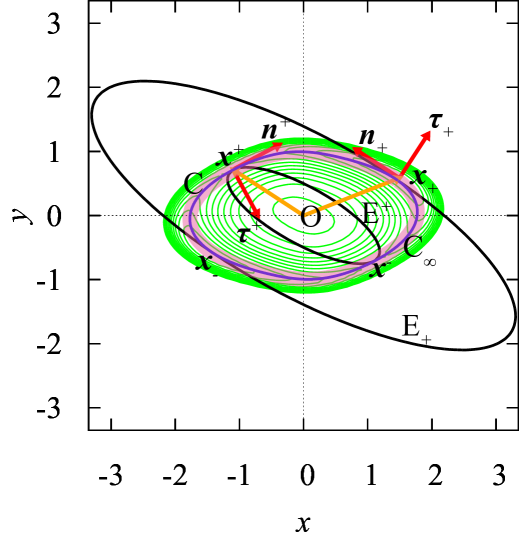
Figure 1: (Color online) Contour plot of $V_{0}(\boldsymbol{x})$ with a skeleton of curves $\mathrm{C}_{\infty}:\{\boldsymbol{x}\mid v_{0}(\boldsymbol{x})=1\}$, $\mathrm{E}_{+}:\{\boldsymbol{x}\mid v_{1}(\boldsymbol{x})=E_{+}\}$ and $\mathrm{E}^{+}:\{\boldsymbol{x}\mid v_{1}(\boldsymbol{x})=E^{+}\}$. The parameters of $V_{0}(\boldsymbol{x})$ are $(m,a,b,K,d,e,f,\lambda,\alpha,\beta)=(2,1.8,1,0.02396,3,8,1,0.27,0.34\pi,0.05\pi)$ (the “$d=3$” row of B1 in Table 2), for which $E_{+}=13.7888$ and $E^{+}=1.78493$. The tangent points between $\mathrm{C}_{\infty}$ and $\mathrm{E}_{+}$ ($\mathrm{E}^{+}$) almost agree with the local minima (saddles) of $V_{0}(\boldsymbol{x})$, i.e., $\boldsymbol{x}_{+}$ and $-\boldsymbol{x}_{+}$ ($\boldsymbol{x}^{+}$ and $-\boldsymbol{x}^{+}$), and so do the valleys $\mathrm{C}$ and $\mathrm{C}_{\infty}$. $\{\boldsymbol{n}_{+},\boldsymbol{\tau}_{+}\}$ ($\{\boldsymbol{n}^{+},\boldsymbol{\tau}^{+}\}$) denote the eigenvectors of $\hat{G}_{0}(\boldsymbol{x})$ at the minima (saddles), which also almost agree with the common tangent and normal vectors, i.e., $\{\boldsymbol{n}_{v},\boldsymbol{\tau}_{v}\}$, between $\mathrm{C}_{\infty}$ and $\mathrm{E}_{+}$ ($\mathrm{C}_{\infty}$ and $\mathrm{E}^{+}$).

For $V_{0}(\boldsymbol{x})$ in Eq. (10), let us consider a ratchet potential with a two-fold symmetry as shown in Fig. 1, and call it the two-tooth ratchet model. In such a case, $v_{0}(\boldsymbol{x})$ and $v_{1}(\boldsymbol{x})$ also have two-fold symmetry. Here, we define them as

$$v_{0}(\boldsymbol{x}) =\lvert\boldsymbol{a}\cdot\boldsymbol{x}\lvert^{2}+\lambda\frac{\lvert\boldsymbol{e}\cdot\boldsymbol{x}\rvert^{2}\lvert\boldsymbol{e}_{\perp}\cdot\boldsymbol{x}\rvert^{2}}{\lvert\boldsymbol{x}\rvert^{2}},$$ (11)

$$v_{1}(\boldsymbol{x}) =\frac{1}{2}\lvert\boldsymbol{d}\cdot\boldsymbol{x}\rvert^{2},$$ (12)

where $\boldsymbol{a}$, $\boldsymbol{d}$, $\boldsymbol{e}$, and $\boldsymbol{e}_{\perp}$ are complex vector-valued parameters:

$$\boldsymbol{a}=\begin{pmatrix}\frac{1}{a}\\ \frac{i}{b}\end{pmatrix},\quad\boldsymbol{e}=\begin{pmatrix}\cos\beta&-\sin\beta\\ \sin\beta&\cos\beta\end{pmatrix}\begin{pmatrix}\frac{1}{e}\\ \frac{i}{f}\end{pmatrix},$$

$$\boldsymbol{e}_{\perp}=\begin{pmatrix}0&-1\\ 1&0\end{pmatrix}\boldsymbol{e},\quad\boldsymbol{d}\equiv\begin{pmatrix}\cos\alpha&-\sin\alpha\\ \sin\alpha&\cos\alpha\end{pmatrix}\begin{pmatrix}d\\ i\end{pmatrix},$$

with $i^{2}=-1$, $a>0$, $b>0$, $e\geq 0$, $f\geq 0$, and $0\leq\beta<\frac{\pi}{4}$.

We assume $m\gg 1$ and $0<K\ll 1$ in Eq. (10), unless stated otherwise. Then, the curve $\mathrm{C}_{\infty}:\{\boldsymbol{x}\mid v_{0}(\boldsymbol{x})=1\}$ approximately indicates the potential valley. If $\lambda=0$, $\mathrm{C}_{\infty}$ is an ellipse, i.e., $\lvert\boldsymbol{a}\cdot\boldsymbol{x}\rvert^{2}=(\boldsymbol{a}\cdot\boldsymbol{x})(\boldsymbol{a}^{\ast}\cdot\boldsymbol{x})=\left(\frac{x}{a}\right)^{2}+\left(\frac{y}{b}\right)^{2}=1$, otherwise, for $\lambda\neq 0$, it adds a fourth harmonic deformation, with reference axes $(\cos\beta,\sin\beta)^{\mathrm{T}}$ and $(-\sin\beta,\cos\beta)^{\mathrm{T}}$. The sharpness of the potential profile normal to $\mathrm{C}_{\infty}$ is tuned by $m$ (as shown in Sec. II.2, the curvature is proportional to $m^{2}$ for $m\geq 1$). Function $v_{1}(\boldsymbol{x})$ is a potential function with an anisotropic axis $(\cos\alpha,\sin\alpha)^{\mathrm{T}}$. The curve of $\lvert\boldsymbol{d}\cdot\boldsymbol{x}\rvert^{2}=\mathrm{constant}$ is an ellipse whose short axis is along $(\cos\alpha,\sin\alpha)^{\mathrm{T}}$ and whose eccentricity is $\sqrt{1-d^{-2}}$ ($d>1$). If $\mathrm{C}_{\infty}$ does not have line symmetry with respect to the anisotropic axis, the pathway along the valley has a ratchet property.

II.1 Features of the potential function

Let $\mathrm{O}$, $\mathrm{C}$, $\boldsymbol{x}_{\sigma}$ ($\sigma\in\{-,+\}$), and $\boldsymbol{x}^{\mu}$ ($\mu\in\{-,+\}$) be the origin, the potential valley of $V_{0}(\boldsymbol{x})$, the local minimum, and the saddle, respectively (Fig. 1) [ $\boldsymbol{x}_{+}$ and $\boldsymbol{x}^{+}$ are placed in $x>0$ and $y>0$, and $\boldsymbol{x}_{-}=-\boldsymbol{x}_{+}$ and $\boldsymbol{x}^{-}=-\boldsymbol{x}^{+}$].

The minima and saddles satisfy $\partial_{\boldsymbol{x}}V_{0}(\boldsymbol{x})=\boldsymbol{0}$, and Eq. (10) leads to

$$\frac{m}{2}\left[1-\left\{v_{0}(\boldsymbol{x})\right\}^{m}\right]\left\{v_{0}(\boldsymbol{x})\right\}^{m-1}\partial_{\boldsymbol{x}}v_{0}(\boldsymbol{x})+K\partial_{\boldsymbol{x}}v_{1}(\boldsymbol{x})=\boldsymbol{0}.$$ (13)

Using the orthogonal vectors

$$\boldsymbol{\tau}_{v}\equiv\frac{\partial_{\boldsymbol{x}}v_{0}(\boldsymbol{x})}{\lvert\partial_{\boldsymbol{x}}v_{0}(\boldsymbol{x})\rvert},\quad\boldsymbol{n}_{v}\equiv\begin{pmatrix}0&-1\\ 1&0\end{pmatrix}\boldsymbol{\tau}_{v},$$ (14)

we decompose Eq. (13) in two directions as

$$\frac{m}{2}\left[1-\left\{v_{0}(\boldsymbol{x})\right\}^{m}\right]\left\{v_{0}(\boldsymbol{x})\right\}^{m-1}=-K\frac{\boldsymbol{\tau}_{v}\cdot\partial_{\boldsymbol{x}}v_{1}(\boldsymbol{x})}{\lvert\partial_{\boldsymbol{x}}v_{0}(\boldsymbol{x})\rvert},$$ (15)

$$\boldsymbol{n}_{v}\cdot\partial_{\boldsymbol{x}}v_{1}(\boldsymbol{x})=0.$$ (16)

When taking the limit $m\rightarrow\infty$ in Eqs. (15) and (16), the minima and the saddles, $\{\boldsymbol{x}_{\sigma},\boldsymbol{x}^{\mu}\}$, satisfy

$$\boldsymbol{n}_{v}\cdot\partial_{\boldsymbol{x}}v_{1}(\boldsymbol{x})=0,\quad\boldsymbol{x}\in\mathrm{C}_{\infty}.$$ (17)

For a geometrical interpretation of Eq. (17), let us define $\mathrm{E}:\{\boldsymbol{x}\mid v_{1}(\boldsymbol{x})=E\}$ as a family of curves specified by the parameter $E$. Then, Eq. (17) means that with certain values of $E$, the curves $\mathrm{E}$ and $\mathrm{C}_{\infty}$ have tangent points at $\boldsymbol{x}\in\{\boldsymbol{x}_{\sigma},\boldsymbol{x}^{\mu}\}$ at which $\boldsymbol{n}_{v}$ is tangent to both curves. As shown in Fig. 1, there are two cases of tangency depending on $E$; let $\mathrm{E}_{+}:\{\boldsymbol{x}\mid v_{1}(\boldsymbol{x})=E_{+}\}$ [ $\mathrm{E}^{+}:\{\boldsymbol{x}\mid v_{1}(\boldsymbol{x})=E^{+}\}$] be a curve that is tangent to $\mathrm{C}_{\infty}$ at $\boldsymbol{x}=\boldsymbol{x}_{\sigma}$ [$\boldsymbol{x}=\boldsymbol{x}^{\mu}$] as $E$ reaches $E_{+}$ [$E^{+}$]. Since we choose $K>0$, we have $E^{+}\leq E_{+}$. Therefore, $\mathrm{E}_{+}$ is externally tangent to $\mathrm{C}_{\infty}$, and $\mathrm{E}^{+}$ is internally tangent to $\mathrm{C}_{\infty}$. However, these describe only the local relationships between $v_{0}(\boldsymbol{x})$ and $v_{1}(\boldsymbol{x})$ at $\boldsymbol{x}=\boldsymbol{x}_{\sigma}$ ($E=E^{+}$) and $\boldsymbol{x}^{\mu}$ ($E^{+}$) as they contact; the global relationships between them remain undefined. As global conditions in which $\mathrm{E}_{+}$ ($\mathrm{E}^{+}$) contacts with $\mathrm{C}_{\infty}$ only at two points $\boldsymbol{x}=\boldsymbol{x}_{+}$ and $\boldsymbol{x}_{-}$ ($\boldsymbol{x}=\boldsymbol{x}^{+}$ and $\boldsymbol{x}^{-}$), we insist that all points on $\mathrm{C}_{\infty}$ satisfy

$$E^{+}\leq v_{1}(\boldsymbol{x})\leq E_{+},$$ (18)

where equal cases of the left and right sides hold at $\boldsymbol{x}=\boldsymbol{x}^{\mu}$ and $\boldsymbol{x}_{\sigma}$, respectively. In this case, letting $\Delta V$ be the difference of $V_{0}(\boldsymbol{x})$ [Eq. (10)] between the saddle and the local minimum, we have

$$\Delta V=K(E_{+}-E^{+}).$$ (19)

II.2 Hessian matrix

The Hessian matrix $\hat{G}_{0}(\boldsymbol{x})\equiv\partial_{\boldsymbol{x}}\partial_{\boldsymbol{x}}^{\mathrm{T}}V_{0}(\boldsymbol{x})$ is diagonalized approximately for $m\gg 1$. We denote its eigenvectors by $\boldsymbol{n}(\boldsymbol{x})$ and $\boldsymbol{\tau}(\boldsymbol{x})$, i.e.,

$$\hat{G}_{0}(\boldsymbol{x})\boldsymbol{\tau}(\boldsymbol{x}) =\Lambda_{\tau}(\boldsymbol{x})\boldsymbol{\tau}(\boldsymbol{x}),$$ (20)

$$\hat{G}_{0}(\boldsymbol{x})\boldsymbol{n}(\boldsymbol{x}) =\Lambda_{n}(\boldsymbol{x})\boldsymbol{n}(\boldsymbol{x}),$$ (21)

where $\Lambda_{n}(\boldsymbol{x})$ and $\Lambda_{\tau}(\boldsymbol{x})$ are the corresponding eigenvalues, respectively; $\boldsymbol{n}(\boldsymbol{x})$ and $\boldsymbol{\tau}(\boldsymbol{x})$ are tangent and normal to $\mathrm{C}$ at $\boldsymbol{x}\in\{\boldsymbol{x}_{\sigma},\boldsymbol{x}^{\mu}\}$; $\Lambda_{n}(\boldsymbol{x})$ and $\Lambda_{\tau}(\boldsymbol{x})$ are equivalent to the curvatures of $V_{0}(\boldsymbol{x})$ along the $\boldsymbol{n}(\boldsymbol{x})$ and $\boldsymbol{\tau}(\boldsymbol{x})$ axes, respectively. Hereinafter, we denote these eigenvectors by $\boldsymbol{n}(\boldsymbol{x}_{\sigma})\equiv\boldsymbol{n}_{\sigma}$, $\boldsymbol{\tau}(\boldsymbol{x}_{\sigma})\equiv\boldsymbol{\tau}_{\sigma}$, $\boldsymbol{n}(\boldsymbol{x}^{\mu})\equiv\boldsymbol{n}^{\mu}$, and $\boldsymbol{\tau}(\boldsymbol{x}^{\mu})\equiv\boldsymbol{\tau}^{\mu}$. In addition, we define the reference direction of $\boldsymbol{n}_{\sigma}$ ($\boldsymbol{n}^{\mu}$) as directed in the counterclockwise (clockwise) pathway of $\mathrm{C}$, and $\boldsymbol{\tau}_{\sigma}$ ($\boldsymbol{\tau}^{\mu}$) as directed in the right-hand side of $\boldsymbol{n}_{\sigma}$ ($\boldsymbol{n}^{\mu}$) (see Fig. 1).

From Eq. (10), we have

$$\hat{G}_{0}(\boldsymbol{x})= -\frac{m}{2}\left[m-1-(2m-1)v_{0}(\boldsymbol{x})^{m}\right]v_{0}(\boldsymbol{x})^{m-2}\partial_{\boldsymbol{x}}v_{0}(\boldsymbol{x})\partial_{\boldsymbol{x}}^{\mathrm{T}}v_{0}(\boldsymbol{x})$$

$$-\frac{m}{2}\left[1-v_{0}(\boldsymbol{x})^{m}\right]v_{0}(\boldsymbol{x})^{m-1}\partial_{\boldsymbol{x}}\partial_{\boldsymbol{x}}^{\mathrm{T}}v_{0}(\boldsymbol{x})-K\partial_{\boldsymbol{x}}\partial_{\boldsymbol{x}}^{\mathrm{T}}v_{1}(\boldsymbol{x}).$$ (22)

Substituting $v_{0}(\boldsymbol{x})=1$ into the first two factors in the first term in Eq. (22), and $v_{0}(\boldsymbol{x})=1+\delta v_{0}$ into the second term, we approximate $\hat{G}_{0}(\boldsymbol{x})$ as

$$\hat{G}_{0}(\boldsymbol{x})\approx \frac{m^{2}}{2}\lvert\partial_{\boldsymbol{x}}v_{0}(\boldsymbol{x})\rvert^{2}\boldsymbol{\tau}_{v}\boldsymbol{\tau}_{v}^{\mathrm{T}}+\frac{m^{2}}{2}\delta v_{0}\partial_{\boldsymbol{x}}\partial_{\boldsymbol{x}}^{\mathrm{T}}v_{0}(\boldsymbol{x})-K\partial_{\boldsymbol{x}}\partial_{\boldsymbol{x}}^{\mathrm{T}}v_{1}(\boldsymbol{x}),$$ (23)

where $\boldsymbol{\tau}_{v}$ is defined in Eq. (14), and, from Eq. (15), $\delta v_{0}$ is estimated as

$$\delta v_{0}\approx\frac{2K\boldsymbol{\tau}_{v}\cdot\partial_{\boldsymbol{x}}v_{1}(\boldsymbol{x})}{m^{2}\lvert\partial_{\boldsymbol{x}}v_{0}(\boldsymbol{x})\rvert}.$$ (24)

From Eqs. (23) and (24), neglecting the nondiagonal components (which are not essential), we obtain

$$\hat{G}_{0}(\boldsymbol{x})\approx\frac{m^{2}}{2}\lvert\partial_{\boldsymbol{x}}v_{0}(\boldsymbol{x})\rvert^{2}\boldsymbol{\tau}_{v}\boldsymbol{\tau}_{v}^{\mathrm{T}}+Kg(\boldsymbol{x})\boldsymbol{n}_{v}\boldsymbol{n}_{v}^{\mathrm{T}},$$ (25)

$$g(\boldsymbol{x})\equiv\boldsymbol{n}_{v}^{\mathrm{T}}\left[\left\{\boldsymbol{\tau}_{v}\cdot\partial_{\boldsymbol{x}}v_{1}(\boldsymbol{x})\right\}\frac{\partial_{\boldsymbol{x}}\partial_{\boldsymbol{x}}^{\mathrm{T}}v_{0}(\boldsymbol{x})}{\lvert\partial_{\boldsymbol{x}}v_{0}(\boldsymbol{x})\rvert}-\partial_{\boldsymbol{x}}\partial_{\boldsymbol{x}}^{\mathrm{T}}v_{1}(\boldsymbol{x})\right]\boldsymbol{n}_{v}$$ (26)

for $\boldsymbol{x}\in\{\boldsymbol{x}_{\sigma},\boldsymbol{x}^{\mu}\}$. This is valid for $m\gg 1$, in which the eigenvectors of the Hessian matrix at $\boldsymbol{x}\in\{\boldsymbol{x}_{\sigma},\boldsymbol{x}^{\mu}\}$, i.e., $\boldsymbol{\tau}_{\sigma}$, $\boldsymbol{n}_{\sigma}$, $\boldsymbol{\tau}^{\mu}$ and $\boldsymbol{n}^{\mu}$, are well approximated with $\boldsymbol{\tau}_{v}$ and $\boldsymbol{n}_{v}$ in Eq. (14). We thus have

$$\Lambda_{\tau}(\boldsymbol{x})\approx\frac{m^{2}}{2}\lvert\partial_{\boldsymbol{x}}v_{0}(\boldsymbol{x})\rvert^{2},\quad\Lambda_{n}(\boldsymbol{x})\approx Kg(\boldsymbol{x})$$ (27)

at $\boldsymbol{x}\in\{\boldsymbol{x}_{\sigma},\boldsymbol{x}^{\mu}\}$ for $m\gg 1$.

III Performance indexes

We characterize the rotational-motion performance of the 2D ratchet using the mean angular momentum (MAM)

$$L\equiv\overline{X_{t}\dot{Y}_{t}-Y_{t}\dot{X}_{t}},$$ (28)

the mean angular velocity (MAV) $\omega\equiv\overline{\dot{\Theta}_{t}}$, and the efficiency

$$\eta=\frac{\gamma L\omega+P_{I}}{P_{h}},$$ (29)

where

$$\Theta_{t}\equiv\int_{0}^{t}ds\left(\frac{X_{s}\dot{Y}_{s}-Y_{s}\dot{X}_{s}}{\lvert\boldsymbol{X}\rvert^{2}}\right)\equiv\theta(\boldsymbol{X})-\theta(\boldsymbol{X}_{0}),$$ (30)

$$P_{I}\equiv-\overline{\dot{\boldsymbol{X}}\cdot\boldsymbol{f}_{I}(\boldsymbol{X})}=\frac{I}{2\pi}\overline{\dot{\theta}(\boldsymbol{X})}=\frac{I\omega}{2\pi},$$ (31)

$$P_{h}\equiv\overline{h\boldsymbol{N}_{t}\cdot\dot{\boldsymbol{X}}(t)},$$ (32)

i.e., the counterclockwise displacement angle about the origin, the power consumed by the load, and the input power of the external field (which is equivalent to the total power consumption), respectively. We have replaced Eq. (9) with Eq. (29) because the long-time averages of the relative angular momentum $L_{t}^{\prime}$ [Eq. (6)] and the relative angular velocity $\omega_{t}^{\prime}$ [Eq. (7)] agree with $L$ and $\omega$, respectively, to $o(h^{2})$ (see Appendix C.3). Hereinafter, $O(\cdot)$ and $o(\cdot)$ denote the Landau symbols (Big- and Little-O).

In Eq. (28), the direction $L>0$ corresponds to counterclockwise rotation. The direction of the ratchet (chirality) is defined as the direction in which one goes around a circular pathway along $\mathrm{C}$ through each of the minima from the side of steeper gradient to the more gentle one. Hence, the ratchet in Fig. 1 has counterclockwise chirality. In the following analytical and numerical simulation results, under the RDDF, the net rotation of the ratchet tends to be the same as the chirality. In the numerical simulations, we examine only the case of $I=0$ and we treat the efficiency as

$$\eta=\frac{\gamma L\omega}{P_{h}}.$$ (33)

In this paper, we consider a ratchet system in a thermal bath under a weak and slow external field, and we impose the following requirements: 1) the typical magnitudes of $V_{h}(\boldsymbol{x},t)$ and $I$ (which are denoted by $O(h)$ and $O(I)$, respectively, in an energetic dimension) are smaller than the energy barrier $\Delta V$ [see Eq. (19)] to a sufficient extent, it being assumed hereinafter that $O(I)\sim O(h)$; 2) the mean switching time of the RDDF ($T_{p}\equiv\frac{2\pi}{\Omega}$) is longer than the typical relaxation time $T_{r}$ of a trajectory to a sufficient extent, i.e., $\Omega T_{r}\ll 1$, where $T_{r}^{-1}$ is related to the curvature of $V_{0}(\boldsymbol{x})$ at the minima [or more likely is governed by the smallest eigenvalue of $\hat{G}_{0}(\boldsymbol{x}_{\sigma})$].

In a previous paper Tutu et al. (2015), we proposed a framework for obtaining approximate expressions for the performance indexes ($L$, $\omega$, and $P_{h}$) using a master equation for coarse-grained states under the assumptions mentioned above. For a self-contained description, we briefly introduce the basic construction of the master equation and its applications to the computation of $L$, $\omega$, and $P_{h}$ in Secs. III.1 and III.2. In Sec. III.3, we show the final expressions for $L$, $\omega$, and $P_{h}$ that we use in later sections.

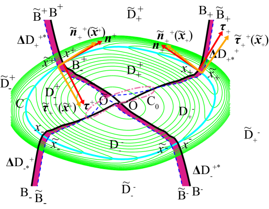
Figure 2: (Color online) Notation for moving domain boundaries on $V(\boldsymbol{x},t)$. With $\sigma\in\{-,+\}$ and $\mu\in\{-,+\}$, $\tilde{\mathrm{O}}$, $\tilde{\boldsymbol{x}}_{\sigma}$, and $\tilde{\boldsymbol{x}}^{\mu}$ represent the local maximum, the local minimum, and the saddle points, respectively, of $V(\boldsymbol{x},t)$. The 2D space is divided into four domains $\tilde{\mathrm{D}}_{\sigma}^{\mu}$ by the ridge curves $\tilde{\mathrm{B}}_{\sigma}$ and $\tilde{\mathrm{B}}^{\mu}$ of $V(\boldsymbol{x},t)$. $\tilde{\boldsymbol{\tau}}_{\sigma}^{\mu}(\tilde{\boldsymbol{x}}_{\sigma})$ and $\tilde{\boldsymbol{\tau}}_{\sigma}^{\mu}(\tilde{\boldsymbol{x}}^{\mu})$ [$\tilde{\boldsymbol{n}}_{\sigma}^{\mu}(\tilde{\boldsymbol{x}}_{\sigma})$ and $\tilde{\boldsymbol{n}}_{\sigma}^{\mu}(\tilde{\boldsymbol{x}}^{\mu})$] are the tangent (normal) vectors to $\tilde{\mathrm{B}}_{\sigma}$ and $\tilde{\mathrm{B}}^{\mu}$ at the minimum and the saddle points. $\mathrm{C}_{0}$ (dashed–dotted curve) denotes a closed curve surrounding a central region of the potential that at least includes $\mathrm{O}$, $\tilde{\mathrm{O}}^{\prime}$ and either a cross point between $\mathrm{B}_{\sigma}$ and $\tilde{\mathrm{B}}_{\sigma}$, or another between $\mathrm{B}^{\mu}$ and $\tilde{\mathrm{B}}^{\mu}$. $\Delta\mathrm{D}_{\sigma\ast}^{\mu}$ [$\Delta\mathrm{D}_{\sigma}^{\mu\ast}$] (hatched regions) denotes the region surrounded by $\tilde{\mathrm{B}}_{\sigma}$ and $\mathrm{B}^{\mu}$ [$\tilde{\mathrm{B}}^{\mu}$ and $\mathrm{B}_{\mu}$] but excluding the interior of $\mathrm{C}_{0}$.

III.1 Coarse-grained states and related definitions

As shown in Fig. 2, we denote $\mathrm{O}$, $\boldsymbol{x}_{\sigma}$, and $\boldsymbol{x}^{\mu}$ ($\sigma\in\{+,-\}$ and $\mu\in\{+,-\}$) as the origin, the local minimum, and the saddle, respectively, determined by $\partial_{\boldsymbol{x}}V_{0}(\boldsymbol{x})=\boldsymbol{0}$. Hereinafter, the signs “$+$” and “$-$” are identical with $+1$ and $-1$, thereby $\boldsymbol{x}_{\sigma}=\sigma\boldsymbol{x}_{+}$ and $\boldsymbol{x}^{\mu}=\mu\boldsymbol{x}^{+}$, where $\boldsymbol{x}_{+}$ and $\boldsymbol{x}^{+}$ lie in $x>0$ and $y>0$, respectively. Furthermore, $\mathrm{B}_{\sigma}$ ($\mathrm{B}^{\mu}$) denotes the ridge curve running from $\mathrm{O}$ through $\boldsymbol{x}_{\sigma}$ ($\boldsymbol{x}^{\mu}$) outward; $\mathrm{D}_{\sigma}^{\mu}$ denotes the domain surrounded by $\mathrm{B}_{\sigma}$ and $\mathrm{B}^{\mu}$; $\mathrm{C}$ denotes the potential valley of $V_{0}(\boldsymbol{x})$.

We extend these static ridge curves to temporally varying ridge curves on the basis of the function

$$V(\boldsymbol{x},t)\equiv V_{0}(\boldsymbol{x})+V_{h}(\boldsymbol{x},t)+\frac{I}{2\pi}\theta(\boldsymbol{x})$$ (34)

with the second and third terms in Eqs. (2) and (4); $\tilde{\mathrm{O}}$, $\tilde{\boldsymbol{x}}_{\sigma}$, and $\tilde{\boldsymbol{x}}^{\mu}$ denote the local maximum, the local minimum, and the saddle (Fig. 2) given by $\partial_{\boldsymbol{x}}V(\boldsymbol{x},t)=\boldsymbol{0}$, respectively, which move temporally with the external field. Similarly, $\tilde{\mathrm{B}}_{\sigma}$ ($\tilde{\mathrm{B}}^{\mu}$) denotes the ridge curves running from $\tilde{\mathrm{O}}$ through $\tilde{\boldsymbol{x}}_{\sigma}$ ($\tilde{\boldsymbol{x}}^{\mu}$) outward; $\tilde{\mathrm{D}}_{\sigma}^{\mu}$ denotes the domain surrounded by $\tilde{\mathrm{B}}_{\sigma}$ and $\tilde{\mathrm{B}}^{\mu}$; $\tilde{\mathrm{C}}$ denotes the potential valley of $V(\boldsymbol{x},t)$.

Corresponding to $\boldsymbol{\tau}(\boldsymbol{x})$ and $\boldsymbol{n}(\boldsymbol{x})$ in Eqs. (20) and (21), we denote by $\tilde{\boldsymbol{\tau}}_{\sigma}^{\mu}(\boldsymbol{x})$ and $\tilde{\boldsymbol{n}}_{\sigma}^{\mu}(\boldsymbol{x})$ the tangent and normal vectors at the point $\boldsymbol{x}$ on the boundary of $\tilde{\mathrm{D}}_{\sigma}^{\mu}$ ($\boldsymbol{x}\in\tilde{\mathrm{B}}_{\sigma}$ or $\boldsymbol{x}\in\tilde{\mathrm{B}}^{\mu}$), where the reference direction of $\tilde{\boldsymbol{n}}_{\sigma}^{\mu}(\boldsymbol{x})$ lies in $\tilde{\mathrm{D}}_{\sigma}^{\mu}$, and $\tilde{\boldsymbol{\tau}}_{\sigma}^{\mu}(\boldsymbol{x})$ is oriented in the right-hand direction of $\tilde{\boldsymbol{n}}_{\sigma}^{\mu}(\boldsymbol{x})$ (Fig. 2). The vectors $\tilde{\boldsymbol{\tau}}_{\sigma}^{\mu}(\boldsymbol{x})$ and $\tilde{\boldsymbol{n}}_{\sigma}^{\mu}(\boldsymbol{x})$ are the eigenvectors of the Hessian matrix $\hat{G}(\boldsymbol{x})\equiv\partial_{\boldsymbol{x}}\partial_{\boldsymbol{x}}^{\mathrm{T}}V(\boldsymbol{x},t)$, i.e.,

$$\hat{G}(\boldsymbol{x})\tilde{\boldsymbol{\tau}}_{\sigma}^{\mu}(\boldsymbol{x}) =\Lambda_{\tau}(\boldsymbol{x})\tilde{\boldsymbol{\tau}}_{\sigma}^{\mu}(\boldsymbol{x}),$$ (35)

$$\hat{G}(\boldsymbol{x})\tilde{\boldsymbol{n}}_{\sigma}^{\mu}(\boldsymbol{x}) =\Lambda_{n}(\boldsymbol{x})\tilde{\boldsymbol{n}}_{\sigma}^{\mu}(\boldsymbol{x}),$$ (36)

where $\Lambda_{\tau}(\boldsymbol{x})$ and $\Lambda_{n}(\boldsymbol{x})$ are the corresponding eigenvalues. In particular, at $\boldsymbol{x}\in\{\tilde{\boldsymbol{x}}_{\sigma},\tilde{\boldsymbol{x}}^{\mu}\}$, $\Lambda_{\tau}(\boldsymbol{x})$ and $\Lambda_{n}(\boldsymbol{x})$ are the curvatures of $V(\boldsymbol{x},t)$ along the ridge curve and the valley, respectively; therefore, we have $\Lambda_{\tau}(\tilde{\boldsymbol{x}}_{\sigma})>0$, $\Lambda_{n}(\tilde{\boldsymbol{x}}_{\sigma})>0$, $\Lambda_{\tau}(\tilde{\boldsymbol{x}}^{\mu})>0$, and $\Lambda_{n}(\tilde{\boldsymbol{x}}^{\mu})<0$.

III.2 Master equation for coarse-grained states

The time evolution of probability density function (PDF) $p(\boldsymbol{x},t)$ for $\boldsymbol{X}=\boldsymbol{x}$ obeys the Fokker–Planck equation as

$$\partial_{t}p(\boldsymbol{x},t)=-\partial_{\boldsymbol{x}}\cdot\boldsymbol{J}(\boldsymbol{x},t),$$ (37)

$$\boldsymbol{J}(\boldsymbol{x},t)\equiv\left[-\partial_{\boldsymbol{x}}V(\boldsymbol{x},t)\right]p(\boldsymbol{x},t)-D\partial_{\boldsymbol{x}}p(\boldsymbol{x},t),$$ (38)

where $\partial_{t}\equiv\frac{\partial}{\partial t}$ and $\partial_{\boldsymbol{x}}\cdot\boldsymbol{J}(\boldsymbol{x},t)$ means the 2D divergence of the probability current density.

In terms of $p(\boldsymbol{x},t)$, a probability for an event $\boldsymbol{X}\in\mathrm{D}_{\sigma}^{\mu}$ is given by

$$P(\sigma,\mu,t)\equiv\int_{\boldsymbol{x}\in\mathrm{D}_{\sigma}^{\mu}}d\boldsymbol{x}p(\boldsymbol{x},t).$$ (39)

Using this, probabilities for events $\boldsymbol{X}\in\mathrm{D}_{\sigma}^{+}\cup\mathrm{D}_{\sigma}^{-}$ and $\boldsymbol{X}\in\mathrm{D}_{+}^{\mu}\cup\mathrm{D}_{-}^{\mu}$ are represented as $P(\sigma,t)=\sum_{\mu}P(\sigma,\mu,t)$ and $Q(\mu,t)=\sum_{\sigma}P(\sigma,\mu,t)$, respectively. Furthermore, the conditional probabilities, the relative probabilities of the event $\boldsymbol{X}\in\mathrm{D}_{\sigma}^{\mu}$ under the conditions $\boldsymbol{X}\in\mathrm{D}_{\sigma}^{+}\cup\mathrm{D}_{\sigma}^{-}$ and $\boldsymbol{X}\in\mathrm{D}_{+}^{\mu}\cup\mathrm{D}_{-}^{\mu}$, are defined respectively as

$$P(\sigma\mid\mu,t)\equiv\frac{P(\sigma,\mu,t)}{Q(\mu,t)},\quad Q(\mu\mid\sigma,t)\equiv\frac{P(\sigma,\mu,t)}{P(\sigma,t)}.$$ (40)

In addition to the assumptions 1) $V_{h}\ll\Delta V$ and 2) $\Omega T_{r}\ll 1$, we assume that $D$ is so small that $D\ll\Delta V$ hereinafter. Then, the PDF peaks sharply at $\tilde{\boldsymbol{x}}_{\sigma}$ [=$\boldsymbol{x}_{\sigma}+O(h)$], otherwise almost vanishes in the other region, and the trajectories in the transition between two states $\boldsymbol{X}\in\tilde{\mathrm{D}}_{+}^{\mu}$ and $\boldsymbol{X}\in\tilde{\mathrm{D}}_{-}^{\mu}$ concentrate to $\tilde{\mathrm{C}}$.

From Eqs. (37) and (39), the time derivative of $P(\sigma,\mu,t)$ leads to

$$\partial_{t}P(\sigma,\mu,t)=\int_{\boldsymbol{x}\in\mathrm{D}_{\sigma}^{\mu}}d\boldsymbol{x}\left[-\partial_{\boldsymbol{x}}\cdot\boldsymbol{J}(\boldsymbol{x},t)\right].$$ (41)

We divide the domain of integration $\mathrm{D}_{\sigma}^{\mu}$ into $\tilde{\mathrm{D}}_{\sigma}^{\mu}$ and $\Delta\mathrm{D}_{\sigma}^{\mu}\equiv\mathrm{D}_{\sigma}^{\mu}-\tilde{\mathrm{D}}_{\sigma}^{\mu}$; $\Delta\mathrm{D}_{\sigma}^{\mu}$ consists of two domains $\{\boldsymbol{x}\mid\boldsymbol{x}\in\mathrm{D}_{\sigma}^{\mu},\boldsymbol{x}\notin\tilde{\mathrm{D}}_{\sigma}^{\mu}\}$ and $\{\boldsymbol{x}\mid\boldsymbol{x}\in\tilde{\mathrm{D}}_{\sigma}^{\mu},\boldsymbol{x}\notin\mathrm{D}_{\sigma}^{\mu}\}$. Therefore, $\Delta\mathrm{D}_{\sigma}^{\mu}$ partly possesses a “negative domain” for which the sign of the integral is inverted. From the assumptions $h\ll\Delta V$ and $D\ll\Delta V$, we can regard the PDF as actually vanishing around $\tilde{\mathrm{O}}$ and $\mathrm{O}$, or the interior of $\mathrm{C}_{0}$ in Fig. 2. We can thus consider the region $\Delta\mathrm{D}_{\sigma}^{\mu}$ as a sum of the part surrounded by $\mathrm{B}_{\sigma}$ and $\tilde{\mathrm{B}}_{\sigma}$ excluding the interior of $\mathrm{C}_{0}$, and the other surrounded by $\mathrm{B}^{\mu}$ and $\tilde{\mathrm{B}}^{\mu}$ excluding the interior of $\mathrm{C}_{0}$, as indicated by hatched regions in Fig. 2. Hereinafter, we denote by $\Delta\mathrm{D}_{\sigma\ast}^{\mu}$ the former region, and by $\Delta\mathrm{D}_{\sigma}^{\mu\ast}$ the latter one. Dividing the domain of integration $\mathrm{D}_{\sigma}^{\mu}$ into $\tilde{\mathrm{D}}_{\sigma}^{\mu}$, $\Delta\mathrm{D}_{\sigma\ast}^{\mu}$, and $\Delta\mathrm{D}_{\sigma}^{\mu\ast}$, we have

$$\partial_{t}P(\sigma,\mu,t)\approx \int_{\boldsymbol{x}\in\tilde{\mathrm{D}}_{\sigma}^{\mu}}d\boldsymbol{x}\left[-\partial_{\boldsymbol{x}}\cdot\boldsymbol{J}(\boldsymbol{x},t)\right]$$

$$-\partial_{t}P(\sigma,\mu,t)\bigr{|}_{Q}+\partial_{t}P(\sigma,\mu,t)\bigr{|}_{P},$$ (42)

where $\partial_{t}P(\sigma,\mu,t)\bigr{|}_{Q}\equiv-\int_{\Delta\mathrm{D}_{\sigma}^{\mu\ast}}d\boldsymbol{x}\left[-\partial_{\boldsymbol{x}}\cdot\boldsymbol{J}(\boldsymbol{x},t)\right]$ and $\partial_{t}P(\sigma,\mu,t)\bigr{|}_{P}\equiv\int_{\Delta\mathrm{D}_{\sigma\ast}^{\mu}}d\boldsymbol{x}\left[-\partial_{\boldsymbol{x}}\cdot\boldsymbol{J}(\boldsymbol{x},t)\right]$.

From the assumptions, we can approximate $p(\boldsymbol{x},t)$ with the thermal equilibrium PDF [$\propto e^{-V(\boldsymbol{x},t)/D}$] around the minima of $V(\boldsymbol{x},t)$, and we assume $\boldsymbol{J}(\boldsymbol{x},t)=\boldsymbol{0}$ on $\tilde{\mathrm{B}}_{\sigma}$. Applying this to the first term in Eq. (42), we obtain

$$\int_{\boldsymbol{x}\in\tilde{\mathrm{D}}_{\sigma}^{\mu}}d\boldsymbol{x}\left[-\partial_{\boldsymbol{x}}\cdot\boldsymbol{J}(\boldsymbol{x},t)\right] \approx\int_{\boldsymbol{x}\in\tilde{\mathrm{B}}^{\mu}}d\boldsymbol{x}\,\tilde{\boldsymbol{n}}_{\sigma}^{\mu}(\boldsymbol{x})\cdot\boldsymbol{J}(\boldsymbol{x},t)$$

$$\equiv\left(\delta_{\sigma,-\mu}-\delta_{\sigma,\mu}\right)J^{\mu}(t),$$ (43)

where $J^{\mu}(t)$ represents the probability current from $\tilde{\mathrm{D}}_{\mu}^{\mu}$ to $\tilde{\mathrm{D}}_{-\mu}^{\mu}$. Terms $\partial_{t}P(\sigma,\mu,t)\bigr{|}_{Q}$ and $\partial_{t}P(\sigma,\mu,t)\bigr{|}_{P}$ are considered as follows. For simplicity, we show them for the case $\sigma=\mu$ as

$$\partial_{t}P(\mu,\mu,t)\bigr{|}_{Q} =\int_{\boldsymbol{x}\in\tilde{\mathrm{B}}^{\mu}}\,d\boldsymbol{x}\,\tilde{\boldsymbol{n}}_{\mu}^{\mu}(\boldsymbol{x})\cdot\boldsymbol{J}(\boldsymbol{x},t)-\int_{\boldsymbol{x}\in\mathrm{B}^{\mu}}\,d\boldsymbol{x}\,\boldsymbol{n}^{\mu}(\boldsymbol{x})\cdot\boldsymbol{J}(\boldsymbol{x},t)$$

$$\approx Q(\mu,t)\int_{\boldsymbol{x}\in\mathrm{B}^{\mu}}\,d\boldsymbol{x}\,\frac{\boldsymbol{n}^{\mu}(\boldsymbol{x})\cdot\left[\boldsymbol{J}(\tilde{\boldsymbol{x}}(\boldsymbol{x}),t)-\boldsymbol{J}(\boldsymbol{x},t)\right]}{Q(\mu,t)}$$ (44)

$$\approx Q(\mu,t)\partial_{t}P(\mu\mid\mu,t),$$ (45)

$$\partial_{t}P(\mu,\mu,t)\bigr{|}_{P} \approx P(\mu,t)\int_{\boldsymbol{x}\in\mathrm{B}_{\mu}}\,d\boldsymbol{x}\,\frac{\boldsymbol{n}_{\mu}(\boldsymbol{x})\cdot\boldsymbol{J}(\boldsymbol{x},t)}{P(\mu,t)}$$ (46)

$$\approx P(\mu,t)\partial_{t}Q(\mu\mid\mu,t),$$ (47)

where $\tilde{\boldsymbol{x}}(\boldsymbol{x})$ in Eq. (44) represents a map from a point $\boldsymbol{x}$ on $\mathrm{B}^{\mu}$ to the corresponding nearest point on $\tilde{\mathrm{B}}^{\mu}$. An action of relative current density $\boldsymbol{J}(\tilde{\boldsymbol{x}}(\boldsymbol{x}),t)-\boldsymbol{J}(\boldsymbol{x},t)$ in the integrand in Eq. (44) [Eq. (46), in which $\boldsymbol{J}(\tilde{\boldsymbol{x}}(\boldsymbol{x}),t)=\boldsymbol{0}$ ($\tilde{\boldsymbol{x}}(\boldsymbol{x})\in\tilde{\mathrm{B}}_{\mu}$)] is regarded as increasing $P(\mu\mid\mu,t)$ [decreasing $Q(\mu\mid\mu,t)$] without varying $Q(\mu,t)$ [$P(\mu,t)$].

In consequence, Eq. (42) becomes

$$\partial_{t}P(\sigma,\mu,t)\approx\left(\delta_{\sigma,-\mu}-\delta_{\sigma,\mu}\right)J^{\mu}(t)+J_{\sigma}^{\mu}(t),$$ (48)

$$J_{\sigma}^{\mu}(t)\equiv P(\sigma,t)\partial_{t}Q(\mu\mid\sigma,t)-Q(\mu,t)\partial_{t}P(\sigma\mid\mu,t).$$ (49)

Based on reaction rate theory Hänggi et al. (1990) or Langer’s method Langer (1968), we obtain $J^{\mu}(t)$ in Eq. (43) as

$$J^{\mu}(t)\approx W(-\mu,\mu,t)P(\mu,t)-W(\mu,\mu,t)P(-\mu,t),$$ (50)

$$W(\sigma,\mu,t)\equiv\frac{1}{2\pi}e^{-[V(\boldsymbol{x}^{\mu},t)-V(\boldsymbol{x}_{-\sigma},t)]/D}\sqrt{\frac{\Lambda_{\tau}(\boldsymbol{x}_{-\sigma})\Lambda_{n}(\boldsymbol{x}_{-\sigma})\lvert\Lambda_{n}(\tilde{\boldsymbol{x}}^{\mu})\rvert}{\Lambda_{\tau}(\tilde{\boldsymbol{x}}^{\mu})}},$$ (51)

where $W(-\mu,\mu,t)$ [$W(\mu,\mu,t)$] is the transition probability from a state $\boldsymbol{X}\in\mathrm{D}_{-\mu}$ to a state $\boldsymbol{X}\in\mathrm{D}_{\mu}^{\mu}$ [$\boldsymbol{X}\in\mathrm{D}_{\mu}$ to $\boldsymbol{X}\in\mathrm{D}_{-\mu}^{\mu}$]; $\Lambda_{\tau}(\boldsymbol{x})$ and $\Lambda_{n}(\boldsymbol{x})$ are the eigenvalues of the Hessian matrix $\hat{G}(\boldsymbol{x})$. For details, see Appendix B.

From Eq. (48), the expectation value for the time derivative of a quantity $A(\boldsymbol{X})\equiv A$ can be approximated with the corresponding coarse-grained variable $A(\boldsymbol{x}_{\sigma})\equiv A_{\sigma}$ as

$$\langle\dot{A}\rangle \approx\sum_{\mu}\left(A_{-\mu}-A_{\mu}\right)J^{\mu}(t)+\sum_{\sigma,\mu}A_{\sigma}J_{\sigma}^{\mu}(t),$$ (52)

where $\langle A\rangle=\sum_{\sigma,\mu}A(\boldsymbol{x}_{\sigma})P(\sigma,\mu,t)$, and $A$ is assumed to be a single-valued function of the position. However, the MAM ($L$) and MAV ($\omega$) cannot be expressed straightforwardly as in Eq. (52), e.g., it seems that the idea regarding $\omega$ as being $\sum_{\sigma,\mu}\theta(\boldsymbol{x}_{\sigma})\partial_{t}P(\sigma,\mu,t)$ fails. This may be because the angular momentum and angular velocity are classified as axial vectors that possess information about the rotational direction as well as their magnitudes. Here, apart from Eq. (52), we directly relate $L$ and $\omega$ with the currents $J^{\mu}(t)$ and $J_{\sigma}^{\mu}(t)$ on the basis of physical consideration. For an example with $\omega$, recalling that $J^{\mu}(t)$, $J_{\mu}^{\mu}(t)$, and $-J_{-\mu}^{\mu}(t)$ express the counterclockwise currents through $\mathrm{B}^{\mu}$, $\left\{\theta(\boldsymbol{x}_{-\mu})-\theta(\boldsymbol{x}_{\mu})\right\}J^{\mu}(t)$, $\left\{\theta(\boldsymbol{x}_{-\mu})-\theta(\boldsymbol{x}_{\mu})\right\}J_{\mu}^{\mu}(t)$, and $\left\{\theta(\boldsymbol{x}_{\mu})-\theta(\boldsymbol{x}_{-\mu})\right\}J_{-\mu}^{\mu}(t)$ approximate the phase velocities measured on the pathway from $\theta(\boldsymbol{x}_{\mu})$ to $\theta(\boldsymbol{x}_{-\mu})$ through $\mathrm{B}^{\mu}$.

We represent $L$ and $\omega$ as a superposition of two parts as $L=L^{(I)}+L^{(h)}$ and $\omega=\omega^{(I)}+\omega^{(h)}$, and express each term as

$$L^{(I)} \approx\frac{g_{L}}{2}\sum_{\mu}\left[\boldsymbol{x}^{\mu}\times(\boldsymbol{x}_{-\mu}-\boldsymbol{x}_{\mu})\right]_{z}\overline{J^{\mu}(t)},$$ (53)

$$L^{(h)} \approx g_{L}^{\prime}\sum_{\sigma,\mu}(\boldsymbol{x}_{\sigma}\times\boldsymbol{x}^{\mu})_{z}$$

$$\times\overline{\left[P(\sigma,t)\partial_{t}Q(\mu\mid\sigma,t)-Q(\mu,t)\partial_{t}P(\sigma\mid\mu,t)\right]},$$ (54)

$$\omega^{(I)} \approx\;g_{O}\sum_{\mu}\left[\theta(\boldsymbol{x}_{-\mu})-\theta(\boldsymbol{x}_{\mu})\right]\overline{J^{\mu}(t)},$$ (55)

$$\omega^{(h)} \approx\;g_{O}^{\prime}\sum_{\sigma,\mu}\left[\theta(\boldsymbol{x}_{-\mu})-\theta(\boldsymbol{x}_{\mu})\right]\left(\delta_{\sigma,\mu}-\delta_{\sigma,-\mu}\right)$$

$$\times\overline{\left[P(\sigma,t)\partial_{t}Q(\mu\mid\sigma,t)-Q(\mu,t)\partial_{t}P(\sigma\mid\mu,t)\right]},$$ (56)

where $L^{(I)}$ and $L^{(h)}$, also $\omega^{(I)}$ and $\omega^{(h)}$, come from the two types of current, $J^{\mu}(t)$ and $J_{\sigma}^{\mu}(t)$. Since the coarse-grained variables for the position and velocity vectors are not exact, we employ dimensionless parameters $g_{L}$, $g_{L}^{\prime}$, $g_{O}$, and $g_{O}^{\prime}$ to adjust the approximations to the numerical results; as shown in Sec. V, their actual values are $O(1)$. Each summand in Eq. (53) represents the $z$-component of the angular momentum at $\boldsymbol{x}^{\mu}$ with the position $\boldsymbol{x}^{\mu}$ and the momentum $\frac{1}{2}(\boldsymbol{x}_{-\mu}-\boldsymbol{x}_{\mu})J^{\mu}(t)$, where the latter is the mean of $(\boldsymbol{x}_{-\mu}-\boldsymbol{x}^{\mu})J^{\mu}(t)$ and $(\boldsymbol{x}^{\mu}-\boldsymbol{x}_{\mu})J^{\mu}(t)$. In Eq. (54), we regard the terms $\boldsymbol{x}_{\mu}\times[(\boldsymbol{x}^{\mu}-\boldsymbol{x}_{\mu})J_{\mu}^{\mu}(t)]$ ($\sigma=\mu$) and $\boldsymbol{x}^{\mu}\times[-(\boldsymbol{x}_{-\mu}-\boldsymbol{x}^{\mu})J_{-\mu}^{\mu}(t)]$ ($\sigma=-\mu$) as the counterclockwise angular momentum. The interpretation of each summand in Eqs. (55) and (56) has already been mentioned in the previous paragraph. Note that $\theta(\boldsymbol{x}_{-\mu})-\theta(\boldsymbol{x}_{\mu})=\pi$.

The long time average in Eqs. (54) and (56) reads as

$$\overline{P(\sigma,t)\partial_{t}Q(\mu,t\mid\sigma,t)-Q(\mu,t)\partial_{t}P(\sigma,t\mid\mu,t)}$$

$$= \overline{-P(\sigma,\mu,t)\partial_{t}\ln P(\sigma,t)+P(\sigma,\mu,t)\partial_{t}\ln Q(\mu,t)}$$

$$= \overline{\ln\frac{P(\sigma,t)}{Q(\mu,t)}\partial_{t}P(\sigma,\mu,t)}$$

from Eq. (40) and the partial integration. Substituting this into Eqs. (54) and (56), we obtain

$$L^{(h)} =g_{L}^{\prime}\sum_{\sigma,\mu}(\boldsymbol{x}_{\sigma}\times\boldsymbol{x}^{\mu})_{z}\left(\delta_{\sigma,-\mu}-\delta_{\sigma,\mu}\right)\overline{J^{\mu}(t)\ln\frac{P(\sigma,t)}{Q(\mu,t)}}$$

$$\approx-g_{L}^{\prime}\sum_{\mu}(\boldsymbol{x}_{\mu}\times\boldsymbol{x}^{\mu})_{z}\overline{\left[\ln\frac{P(\mu,t)}{Q(\mu,t)}+\ln\frac{P(-\mu,t)}{Q(\mu,t)}\right]J^{\mu}(t)},$$ (57)

$$\omega^{(h)} \approx-\pi g_{O}^{\prime}\sum_{\mu}\overline{\left[\ln\frac{P(\mu,t)}{Q(\mu,t)}+\ln\frac{P(-\mu,t)}{Q(\mu,t)}\right]J^{\mu}(t)},$$ (58)

where we assume that $J_{\sigma}^{\mu}(t)$ is of higher order in $h$ than $J^{\mu}(t)$ [$\sim O(h)$] in Eqs. (48) and (49).

The mean power consumption $P_{h}$ in Eq. (32) can be written as $\overline{h\boldsymbol{N}_{t}\cdot\langle\dot{\boldsymbol{X}}\rangle}$. Then, $\langle\dot{\boldsymbol{X}}\rangle$ is estimated by applying the first term in Eq. (52) as

$$\langle\dot{\boldsymbol{X}}\rangle\approx g_{V}\sum_{\mu}(\boldsymbol{x}_{-\mu}-\boldsymbol{x}_{\mu})J^{\mu}(t)$$ (59)

with an adjustable parameter $g_{V}$ neglecting the higher-order terms other than $O(h)$, and we obtain

$$P_{h}=-2g_{V}h\sum_{\mu}\overline{J^{\mu}(t)\boldsymbol{N}_{t}}\cdot\boldsymbol{x}_{\mu}.$$ (60)

Calculations for $L^{(I)}$, $L^{(h)}$, $\omega^{(I)}$, $\omega^{(h)}$, and $P_{h}$ are shown in Appendix C.

III.3 Expressions for $L$, $\omega$ and $P_{h}$

From the details given in Appendix C.1 [Eqs. (121)–(128)], we obtain

$$L\approx\frac{g_{L}W_{0}}{2D}\left(\boldsymbol{x}_{+}\times\boldsymbol{x}^{+}\right)_{z}\,\{I_{0}(D)-I\},$$ (61)

$$\omega\approx\frac{\pi g_{O}W_{0}}{2D}\left\{I_{0}(D)-I\right\},$$ (62)

where

$$W_{0} \equiv\frac{1}{2\pi}e^{-[V_{0}(\boldsymbol{x}^{+})-V_{0}(\boldsymbol{x}_{+})]/D}\sqrt{\frac{H_{\tau}H_{n}\lvert G_{n}\rvert}{G_{\tau}}},$$ (63)

$$\approx\frac{K}{2\pi}\frac{\lvert\partial_{\boldsymbol{x}}v_{0}(\boldsymbol{x}_{+})\rvert}{\lvert\partial_{\boldsymbol{x}}v_{0}(\boldsymbol{x}^{+})\rvert}\sqrt{g(\boldsymbol{x}_{+})\lvert g(\boldsymbol{x}^{+})\rvert}e^{-\Delta V/D}\quad(m\gg 1),$$ (64)

$$I_{0}(D) \equiv-\frac{8g_{L}^{\prime}h^{2}\Omega}{g_{L}\sqrt{2\pi DH_{n}}}\frac{\boldsymbol{x}_{+}\cdot\boldsymbol{n}_{+}}{\Omega+4W_{0}},$$ (65)

$$\approx-\frac{8g_{L}^{\prime}h^{2}\Omega}{g_{L}\sqrt{2\pi KDg(\boldsymbol{x}_{+})}}\frac{\boldsymbol{x}_{+}\cdot\boldsymbol{n}_{v}(\boldsymbol{x}_{+})}{\Omega+4W_{0}}\quad(m\gg 1).$$ (66)

Here, $H_{\tau}\equiv\Lambda_{\tau}(\boldsymbol{x}_{\sigma})$, $H_{n}\equiv\Lambda_{n}(\boldsymbol{x}_{\sigma})$, $G_{n}\equiv\Lambda_{n}(\boldsymbol{x}^{\mu})$, and $G_{\tau}\equiv\Lambda_{\tau}(\boldsymbol{x}^{\mu})$ from Eqs. (20) and (21); $g_{L}$, $g_{L}^{\prime}$, and $g_{O}$ are adjustable parameters of $O(1)$. Equations (64) and (66) are obtained from Eqs. (19) and (27).

Equations (61) and (62) suggests that the stimuli of the RDDF can support positive work and torque for the load as long as $I<I_{0}(D)$ ($\gamma L$ is regarded as a viscous torque). Thus, the quantity $\displaystyle\max_{D}{I_{0}(D)}$ indicates the maximal load for such productive work; it quantifies the maximal performance of the ratchet. From Eq. (65), it is found that a higher value of $\displaystyle\max_{D}I_{0}(D)$ is gained if the value of $-\boldsymbol{x}_{+}\cdot\boldsymbol{n}_{+}$ is increased. As shown in Fig. 1, the factor $-\boldsymbol{x}_{+}\cdot\boldsymbol{n}_{+}$ characterizes the asymmetry in the ratchet shape. Additionally, one may anticipate another way of increasing $\displaystyle\max_{D}I_{0}(D)$, namely by decreasing $H_{n}$. However, we note that Eq. (65) is not always valid for small $H_{n}$ either because it eventually conflicts with the prerequisite $\Omega T_{r}\ll 1$ for small $H_{n}$ or, because of the time-dependent fields, the potential with small $H_{n}$ possibly yields temporal minima other than $\{\boldsymbol{x}_{\sigma}\}$. Namely, as $H_{n}$ becomes vanishingly small, the influence of the time-dependent fields becomes relatively strong, possibly breaking the local equilibrium condition on which our theory crucially depends (see Appendix B). So, the effect of decreasing $H_{n}$ may be limited.

From the results in Appendix C.2, we also obtain $P_{h}$ as

$$P_{h}\approx\frac{2g_{V}h^{2}\left|\boldsymbol{x}_{+}\right|^{2}}{D}\frac{\Omega W_{0}}{\Omega+4W_{0}},$$ (67)

where $g_{V}$ is an adjustable parameter.

IV Optimization of ratchet potential

IV.1 Optimization problem

We now consider the problem of maximizing $\omega$ and $L$ through $I_{0}(D)$ by optimizing $V_{0}(\boldsymbol{x})$ [see Eqs. (61)–(65)]. This also has the appreciable effect of increasing $\eta$ through the numerator $L\omega$ in Eq. (29), whereas the optimization of $V_{0}(\boldsymbol{x})$ does not crucially affect the denominator $P_{h}$ according to Eq. (67).

As mentioned in Sec. III, from Eq. (65), we can carry out the maximization of $I_{0}(D)$ by designing $V_{0}(\boldsymbol{x})$ so as to maximize the factor $-\boldsymbol{x}_{+}\cdot\boldsymbol{n}_{+}(\boldsymbol{x}_{+})$, which can be replaced with the approximation $-\boldsymbol{x}_{+}\cdot\boldsymbol{n}_{v}(\boldsymbol{x}_{+})$ for $m\gg 1$ from Eq. (66). In addition to this, we may minimize $H_{n}$ [which corresponds to $g(\boldsymbol{x}_{+})$ in Eq. (66)] within a valid range for the local equilibrium condition around the potential minima. Hereinafter, we assume $m\gg 1$ even in cases in which the essential 2D ratchet characteristics are retained. We then treat $-\boldsymbol{x}_{+}\cdot\boldsymbol{n}_{v}(\boldsymbol{x}_{+})$ as the main objective function to maximize and, if necessary, treat $g(\boldsymbol{x}_{+})$ as an optional objective function to minimize within some limited range.

Thus, a goal of the optimization is to optimize $v_{0}(\boldsymbol{x})$ or $v_{1}(\boldsymbol{x})$ to maximize $-\boldsymbol{x}_{+}\cdot\boldsymbol{n}_{v}(\boldsymbol{x}_{+})$. As shown in Sec. II, functions $v_{0}(\boldsymbol{x})$ and $v_{1}(\boldsymbol{x})$ set up the shape of the potential valley and the local minima and saddles in it. Taking these into account, we first optimize $v_{1}(\boldsymbol{x})$ because it immediately affects $-\boldsymbol{x}_{+}\cdot\boldsymbol{n}_{v}(\boldsymbol{x}_{+})$ through $\boldsymbol{x}_{+}$. Here, let $p$ be a parameter in $v_{1}(\boldsymbol{x})$, and rewrite it as $v_{1}(\boldsymbol{x})\equiv v_{1}(\boldsymbol{x};p)$ to express its dependence on $p$; $\boldsymbol{x}_{+}$ also depends on $p$. In Eq. (12), $p$ corresponds to $\alpha$ or $d$. Then, our problem is to find an optimized value of $p$ ($\equiv p_{\ast}$), i.e.,

$$p_{\ast}\equiv\operatorname*{arg\,max}_{p}\left\{-\boldsymbol{x}_{+}\cdot\boldsymbol{n}_{v}(\boldsymbol{x}_{+})\right\},$$ (68)

where $\boldsymbol{x}_{+}$ ($\in\mathrm{C}_{\infty}$) is subject to $E_{+}=v_{1}(\boldsymbol{x}_{+};p)$ and

$$E^{+}\leq v_{1}(\boldsymbol{x};p)\leq E_{+},\quad\forall\boldsymbol{x}\in\mathrm{C}_{\infty},$$ (69)

with $E^{+}=v_{1}(\boldsymbol{x}^{+};p)$ ($\boldsymbol{x}^{+}\in\mathrm{C}_{\infty}$).

Because this expression is rather complicated for compact wording, an alternative for practical computation is as follows. Here, let us consider $v_{1}(\boldsymbol{x})$ with the specific form $v_{1}(\boldsymbol{x})\equiv\boldsymbol{x}^{\mathrm{T}}\hat{O}_{\alpha}\hat{E}_{d}\hat{O}_{\alpha}^{\mathrm{T}}\boldsymbol{x}$, where

$$\hat{O}_{\alpha}\equiv\begin{pmatrix}\cos\alpha&-\sin\alpha\\ \sin\alpha&\cos\alpha\end{pmatrix},\quad\hat{E}_{d}\equiv\begin{pmatrix}d^{2}&0\\ 0&1\end{pmatrix}.$$ (70)

In the actual procedure, with $\boldsymbol{x}_{+}$ determined in

$$\mathrm{G}_{1}:\ \boldsymbol{x}_{+}=\operatorname*{arg\,max}_{\boldsymbol{x}\in\mathrm{C}_{\infty}}\left\{-\boldsymbol{x}\cdot\boldsymbol{n}_{v}(\boldsymbol{x})\right\},$$ (71)

we fix $(\alpha,d)$ through Eq. (17) or

$$\mathrm{G}_{2}:\ \boldsymbol{n}_{v}^{\mathrm{T}}(\boldsymbol{x}_{+})\hat{O}_{\alpha}\hat{E}_{d}\hat{O}_{\alpha}^{\mathrm{T}}\boldsymbol{x}_{+}=0.$$ (72)

Hereinafter, $\alpha$ and $d$ range as $0\leq\alpha<\frac{\pi}{2}$ and $d>1$, which makes the ratchet direction counterclockwise (see Fig. 1). Note that Eq. (69) is unchanged under $d\rightarrow\frac{1}{d}$, $\alpha\rightarrow\frac{\pi}{2}+\alpha$, $E_{+}\rightarrow\frac{E_{+}}{d^{2}}$, and $E_{-}\rightarrow\frac{E_{-}}{d^{2}}$. So far, either $\alpha$ or $d$ is a free parameter, but not both. For example, using the replacement $d\equiv\tan\delta$ and the matrix $\hat{A}_{\alpha}$ defined as

$$\hat{O}_{\alpha}\hat{E}_{d}\hat{O}_{\alpha}^{\mathrm{T}}=\frac{1+d^{2}}{2}\hat{1}-\frac{1-d^{2}}{2}\hat{A}_{\alpha},\quad\hat{A}_{\alpha}\equiv\begin{pmatrix}\cos 2\alpha&\sin 2\alpha\\ \sin 2\alpha&-\cos 2\alpha\end{pmatrix},$$ (73)

Eq. (72) is read as

$$\mathrm{G}_{2}^{\prime}:\ \cos 2\delta=\frac{-\boldsymbol{n}_{v}(\boldsymbol{x}_{+})\cdot\boldsymbol{x}_{+}}{-\boldsymbol{n}_{v}(\boldsymbol{x}_{+})^{\mathrm{T}}\hat{A}_{\alpha}\boldsymbol{x}_{+}}\quad\left(\frac{\pi}{4}<\delta<\frac{\pi}{2}\right).$$ (74)

This is useful when one chooses $\alpha$ as the free parameter, and determines $\delta$ (also $d$) with $\alpha$. If $d$ is given instead, $\alpha$ is determined by solving Eq. (72).

After determining $\boldsymbol{x}_{+}$ and $(\alpha,d)$, if the right inequality in Eq. (69) is satisfied for $E_{+}=\boldsymbol{x}_{+}^{\mathrm{T}}\hat{O}_{\alpha}\hat{E}_{d}\hat{O}_{\alpha}^{\mathrm{T}}\boldsymbol{x}_{+}$, we settle the (elliptic) curve $\mathrm{E}_{+}$ with these values. Otherwise, if the inequality is unsatisfied, we may search for other values of $\boldsymbol{x}_{+}$ and $(\alpha,d)$, which may be found at the second extreme point $\boldsymbol{x}\in\mathrm{C}_{\infty}$ of $-\boldsymbol{x}\cdot\boldsymbol{n}_{v}(\boldsymbol{x})$, or may refine $v_{0}(\boldsymbol{x})$. This procedure is finalized by finding $\boldsymbol{x}^{+}$ ($\in\mathrm{C}_{\infty}$), which satisfies $\boldsymbol{n}_{v}^{\mathrm{T}}(\boldsymbol{x}^{+})\hat{O}_{\alpha}\hat{E}_{d}\hat{O}_{\alpha}^{\mathrm{T}}\boldsymbol{x}^{+}=0$ and the left inequality in Eq. (69) for $E^{+}=\boldsymbol{x}^{+\mathrm{T}}\hat{O}_{\alpha}\hat{E}_{d}\hat{O}_{\alpha}^{\mathrm{T}}\boldsymbol{x}^{+}$. The curve $\mathrm{E}^{+}$ is also settled with $\boldsymbol{x}^{+}$ and $E^{+}$.

IV.1.1 Elliptic case ($\lambda=0$)

We show analytical results for $L$, $P_{h}$, and $\eta$ maximized by optimizing $v_{1}(\boldsymbol{x})$, through the parameters $\alpha$ and $d$, with $\mathrm{G}_{1}$ [Eq. (71)] and $\mathrm{G}_{2}$ [Eq. (72)] for the elliptic $\mathrm{C}_{\infty}$ ($\lambda=0$) and $m\gg 1$. The maximized expressions for those in Eqs. (61), (64), (66), (67), and (33) are obtained as

$$L\approx\frac{g_{L}abW_{0}}{2D}\{I_{0}(D)-I\},$$ (75)

$$P_{h}\approx\frac{2g_{V}h^{2}(a^{2}+b^{2}-ab)}{D}\frac{\Omega W_{0}}{\Omega+4W_{0}},$$ (76)

$$\eta\approx\frac{2\gamma g_{O}g_{L}^{{}^{\prime}2}h^{2}\{ab(a-b)\}^{2}}{g_{L}g_{V}(a^{2}+b^{2}-ab)\Delta VD^{2}}\frac{\Omega W_{0}}{\Omega+4W_{0}},$$ (77)

where, for $a>b>0$,

$$W_{0}\approx\frac{\Delta V}{\pi(a^{2}+b^{2}-ab)}e^{-\Delta V/D},$$ (78)

$$I_{0}(D)\approx\frac{4g_{L}^{\prime}h^{2}\Omega}{g_{L}\sqrt{\pi\Delta VD}}\frac{\sqrt{ab}(a-b)}{\Omega+4W_{0}},$$ (79)

$$\Delta V=\frac{K}{2}\sqrt{ab}(a+b)(d^{2}-1)\sin(2\alpha).$$ (80)

The details of the above process are given in Appendix D. From Eq. (62), $\omega$ is proportional to $L$. Corresponding to Eq. (72) or (74), $\alpha$ and $d$ ($>1$) are related as

$$\frac{d^{2}+1}{d^{2}-1}=\frac{\sqrt{ab}}{a+b}\sin 2\alpha-\frac{{a}^{2}+{b}^{2}}{a^{2}-b^{2}}\cos 2\alpha.$$ (81)

In the elliptic case, according to Eq. (81), we can choose any value for $\alpha$ unless the prerequisite $\Delta V\gg D$ in the approximation (see Appendix A) is violated. Furthermore, we do not need to minimize $g(\boldsymbol{x}_{+})$ (or to optimize $v_{1}(\boldsymbol{x})$ through $\alpha$). Note that, in the particular case of $\alpha\rightarrow\frac{\pi}{2}$ (or $0$), Eq. (80) leads to $\Delta V\rightarrow 0$, and $\Delta V\gg D$ is violated, where $\mathrm{E}_{+}$ and $\mathrm{E}^{+}$ coincide with $\mathrm{C}_{\infty}$ [$d\rightarrow\frac{a}{b}$ (or $\frac{b}{a}$)].

IV.2 Nonelliptic case ($\lambda\neq 0$)

Here, as a second optimization, we consider a strategy for minimizing $E_{+}$. In the case of $\lambda\neq 0$, the curve $\mathrm{E}_{+}$ never coincides with $\mathrm{C}_{\infty}$ for any $(\alpha,d)$. When minimizing $E_{+}$ with respect to $(\alpha,d)$, $E_{+}>E^{+}$ is retained, and both $\alpha$ and $d$ acquire definitive values. At the minimized $E_{+}$, the two curves $\mathrm{E}_{+}$ and $\mathrm{E}^{+}$ tightly enclose $\mathrm{C}_{\infty}$. This suggests that minimizing $E_{+}$ causes $g(\boldsymbol{x}_{+})$ (corresponding to $H_{n}$) to decrease.

In the case of $\lambda\neq 0$, in addition to the procedure $\mathrm{G}_{1}$ in Eq. (71), firstly, we impose

$$\mathrm{G}_{3}:\quad(\alpha_{\ast},d_{\ast})=\operatorname*{arg\,min}_{0\leq\alpha<\frac{\pi}{2},d(\alpha)>1}E_{+},$$ (82)

where $d(\alpha)$ denotes $d$ as a function of $\alpha$ defined in Eq. (74) [or Eq. (72)]; thus, the essential number of optimization parameters is one. Specifically, after determining $\boldsymbol{x}_{+}$ via $\mathrm{G}_{1}$, from the set of the pairs $(\alpha,d)$ satisfied in $\mathrm{G}_{2}$, $\mathrm{G}_{3}$ selects $\alpha_{\ast}$ and $d_{\ast}$ such that they minimize $E_{+}$ (this automates the tuning of parameters). As mentioned above, the procedure $\mathrm{G}_{3}$ flattens the potential profile along the valley, and narrows the intersection of the valley. It is then expected that the fluctuation of the rotor trajectory may be suppressed within the valley. This accords with our intention to improve the rotational efficiency.

Here, we should note that $\boldsymbol{x}_{+}$ in Eq. (74) has been obtained in the limit $m\rightarrow\infty$ and in the absence of the external fields ($h=0$ and $I=0$). However, the actual minimum point deviates from $\boldsymbol{x}_{+}$; if determining $\boldsymbol{x}_{+}$ with $\partial_{\boldsymbol{x}}V_{0}(\boldsymbol{x})=h\boldsymbol{N}_{t}+\boldsymbol{f}_{I}(\boldsymbol{x})$, Eqs. (15) and (16) are modified. In particular, in the case of $h\neq 0$, $I=0$, and $m\rightarrow\infty$, Eq. (17) is modified as $\boldsymbol{n}_{v}\cdot\partial_{\boldsymbol{x}}v_{1}^{\prime}(\boldsymbol{x},\Phi_{t})=0$ ($\boldsymbol{x}\in\mathrm{C}_{\infty}$) with

$$v_{1}^{\prime}(\boldsymbol{x},\Phi_{t})\equiv v_{1}(\boldsymbol{x})-\frac{h}{K}\boldsymbol{x}\cdot\boldsymbol{N}_{t}$$ (83)

for minima and saddles. In this case, a curve $\mathrm{E}(\Phi_{t}):\{\boldsymbol{x}\mid v_{1}^{\prime}(\boldsymbol{x},\Phi_{t})=E\}$ is the same ellipse as $\mathrm{E}$ except that the center of $\mathrm{E}(\Phi_{t})$ moves around the origin. Because of this movement, the minimum point, at which $\mathrm{E}(\Phi_{t})$ is circumscribed to $\mathrm{C}_{\infty}$, also moves along $\mathrm{C}_{\infty}$. There is a single circumscribed point corresponding to the global minimum and a single inscribed point corresponding to a saddle, which we denote by $\boldsymbol{x}_{\ast t}$ and $\boldsymbol{x}_{t}^{\ast}$, respectively. Similarly, corresponding to Eq. (69), such a minimum and a saddle satisfy $E^{\ast}(\Phi_{t})\leq v_{1}^{\prime}(\boldsymbol{x},\Phi_{t})\leq E_{\ast}(\Phi_{t})$ for $\forall\boldsymbol{x}\in\mathrm{C}_{\infty}$ with $E^{\ast}(\Phi_{t})\equiv v_{1}^{\prime}(\boldsymbol{x}_{t}^{\ast},\Phi_{t})$ and $E_{\ast}(\Phi_{t})\equiv v_{1}^{\prime}(\boldsymbol{x}_{\ast t},\Phi_{t})$.

As the circumscribed ellipse $\mathrm{E}_{\ast}(\Phi_{t}):\{\boldsymbol{x}\mid v_{1}^{\prime}(\boldsymbol{x},\Phi_{t})=E_{\ast}(\Phi_{t})\}$ varies with the external field, $\boldsymbol{x}_{\ast t}$ ($\boldsymbol{x}_{t}^{\ast}$) is not always close to either $\boldsymbol{x}_{+}$ or $\boldsymbol{x}_{-}$ ($\boldsymbol{x}^{+}$ or $\boldsymbol{x}^{-}$). Rather, it may sometimes jump to another point on $\mathrm{C}_{\infty}$ away from them, which creates a temporal minimum. The occurrence of such events depends on the parameters $(\alpha,d)$ or the shape of $\mathrm{C}_{\infty}$. In the experimental observation shown in Sec. V.2, the temporal minimum is likely to arise when $\mathrm{C}_{\infty}$ (of larger $\lambda$) is tightly enclosed by $\mathrm{E}_{+}$ and $\mathrm{E}^{+}$, as a result of optimizing $(\alpha,d)$ in $\mathrm{G}_{3}$. It is also expected that the temporal minimum may become an obstacle in the conversion of power to net rotational output, and may have a negative influence on the efficiency. Therefore, we moderate $\mathrm{G}_{3}$ by adding a relaxation such that the gap between $\mathrm{E}^{+}$ and $\mathrm{E}_{+}$ becomes wider to a sufficient extent. Since $d$ is minimized to $d_{\ast}$ in $\mathrm{G}_{3}$, then, to relax it, we replace $d$ with

$$d=d_{\ast}+\epsilon\quad(\epsilon>0),$$ (84)

where $\epsilon$ is a relaxation parameter. Again applying this $d$ to $\mathrm{G}_{2}$ [Eq. (72)], we obtain a revised $\alpha$. Now, with the ratchet potential of this $(\alpha,d)$, we can expect that the contact point between the ellipse $\mathrm{E}_{+}(\Phi_{t})$ and $\mathrm{C}_{\infty}$ is always close to either $\boldsymbol{x}_{+}$ or $\boldsymbol{x}_{-}$, and that the local equilibrium can be retained.

V Numerical results

Label	Key param. vals.		Fig. 3	$\Delta V$, $K$, and/or $d$.
A1	$\alpha$	$0.03\pi$	(a)	$(K,\Delta V,d)$	$(0.0284,0.1500,d_{0.4\pi})$
		$0.4\pi$	(b)		$(0.102,0.1498,d_{0.4\pi})$
		$0.48\pi$	(c)		$(0.193,0.1501,2.1)$
A2	$(a,b)$	$(1.8,1)$	(b)	$(K,\Delta V)$	$(0.102,0.1498)$
		$(2.7,1.5)$	(d)		$(0.0454,0.1500)$
		$(3.6,2)$	(e)		$(0.0255,0.1500)$
A3	$m$	$1$	(f)	$\Delta V$	$0.1896$
		$2$	(b)		$0.1498$
		$3$	(g)		$0.1436$
A4	$a$	$1.2$	(h)	$(K,\Delta V)$	$(0.672,0.1501)$
		$1.8$	(b)		$(0.102,0.1498)$
		$2.4$	(i)		$(0.038,0.1495)$

Table 1: List of parameter families in the elliptic case ($\lambda=0$). The families are labeled as in the first column, and their key parameters are listed in the second and third columns. The common parameters in each family are as follows: A1: $(m,a,b)=(2,1.8,1)$, A2: $(m,d,\alpha)=(2,d_{0.4\pi},0.4\pi)$, A3: $(a,b,K,d,\alpha)=(1.8,1.0,0.102,d_{0.4\pi},0.4\pi)$, A4: $(m,b,\alpha)=(2,1,0.4\pi)$. In A4, $d$ is determined by Eq. (81) for each $(a,b,\alpha)$. $\Delta V\approx 0.15$ is maintained by modifying $K$ (fifth and sixth columns) except for A3. $d_{0.4\pi}\approx 1.860118$.

We show the numerical results of $L$ (MAM) in Eq. (28), $\omega=\left\langle\frac{\Theta_{T_{\mathrm{tot}}}}{T_{\mathrm{tot}}}\right\rangle_{\Phi}$ (MAV) with $\Theta_{t}$ in Eq. (30), $P_{h}$ in Eq. (32), and $\eta$ in Eq. (33) for several parameter families of $V_{0}(\boldsymbol{x})$. We also discuss the utility of the optimization strategy described in Secs. IV.1 and IV.2. The numerical simulation of Eq. (1) was carried out using the second-order stochastic Runge–Kutta method with a time increment of $0.005$ ($m=1,2$) or $0.002$ ($m=3$). The long time average, $\overline{A(\boldsymbol{X},\Phi_{t})}$, was obtained by averaging $128$ independent trials of the time series of $T_{\mathrm{tot}}\Omega=2^{17}$. Throughout this paper, the parameters of $V_{h}(\boldsymbol{x},t)$ in Eq. (2) are set to $h=0.01$ and $\Omega=0.001$; no load is applied ($I=0$); the fitting parameters in Eqs. (61), (62), (65), and (67) are set to $g_{L}=2.2$, $g_{L}^{\prime}=1.0$, $g_{O}=0.82g_{L}$, and $g_{V}=0.75$.

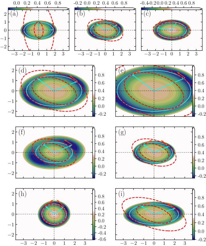
Figure 3: (Color online) Contour graphs of $V_{0}(\boldsymbol{x})$ on $\{\boldsymbol{x}\mid\lvert x\rvert\leq 3.75,\lvert y\rvert\leq 2.5\}$ in the parameter families A1, A2, A3, and A4 in Table 1. In (a), (b), and (c), the locations of the local minima differ (A1); in (b), (d), and (e), the shapes of the elliptic valley have a similarity with the ratio of diameters as $1:2:3$ (A2); in (f), (b), and (g), $m=1$, $2$, and $3$ (A3); in (h), (b), and (i), the eccentricities differ (A4). See the fourth column in Table 1 for the correspondences. The solid and dashed closed curves indicate $\mathrm{C}_{\infty}$, $\mathrm{E}_{+}$ (ellipse circumscribed to $\mathrm{C}_{\infty}$), and $\mathrm{E}^{+}$ (ellipse inscribed to $\mathrm{C}_{\infty}$), respectively. The arrows starting at the origin and ending at the minimum and saddle (near the circumscribed and inscribed points) indicate $\boldsymbol{x}_{+}$ (minimum) and $\boldsymbol{x}^{+}$ (saddle), respectively. The arrows tangent to $\mathrm{C}_{\infty}$ at $\boldsymbol{x}_{+}$ and $\boldsymbol{x}^{+}$ indicate $\boldsymbol{n}_{+}$ and $\boldsymbol{n}^{+}$, respectively.

V.1 Elliptic case ($\lambda=0$)

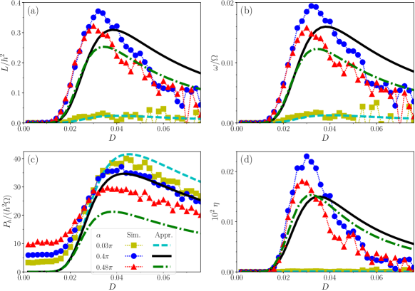
Figure 4: (Color online) (a) Scaled mean angular momentum $L/h^{2}$, (b) scaled mean angular velocity $\omega/\Omega$, (c) scaled input power $P_{h}/(h^{2}\Omega)$, and (d) efficiency $\eta$ versus noise intensity $D$. As shown in the legend box in the lower-right panel, connected symbols ($\Box$, $\bullet$, and $\triangle$) and (dashed, solid, and dotted) curves represent the numerical (Sim.) and approximation (Appr.) results under the potentials of parameter family A1, which are shown in Fig. 3(a)–(c).

We show the outcome of the optimization for the performance indexes according to the parameter families A1–A4 in Table 1, and test the results in Eqs. (75) and (76). The contour graphs of $V_{0}(\boldsymbol{x})$ for the parameter sets in Table 1 are displayed in Fig. 3.

In parameter family A1, it is mainly $\alpha$ that is varied so that the local minima are positioned near the $x$ axis ($\alpha=0.03\pi$) as in Fig. 3(a), the optimized position ($\alpha=0.4\pi$) as in (b), and near the $y$ axis ($\alpha=0.48\pi$) as in (c). In the second case, the factor $-\boldsymbol{x}_{+}\cdot\boldsymbol{n}_{+}$ in $I_{0}(D)$ [Eq. (65)] is maximized with the optimized position $\boldsymbol{x}_{+}$ in Eq. (71), and the parameter $d$ satisfies Eq. (81) [corresponding to Eq. (16) or Eq. (72)]. In contrast, in the first and third cases, $\alpha$ and $d$ do not satisfy Eq. (81). As in Fig. 3(a) and (c), neither $\mathrm{E}_{+}$ nor $\mathrm{E}^{+}$ are tangent to $\mathrm{C}_{\infty}$.

Figure 4 shows the plots of $L$, $\omega$, $P_{h}$, and $\eta$ for $D$ in parameter family A1. The sets of connected symbols and the (dashed, solid, and dashed–dotted) curves represent the results of the numerical simulations (Sim.) and the approximations (Appr.), i.e., Eqs. (61), (62), (67), and (33), respectively (see the legend box for the correspondences between the parameters and the types of symbol or curve). Each of these curves has a peak with respect to $D$ that can be estimated from the relation $\Omega\sim W_{0}$ as the steepest point of the factor $W_{0}/(\Omega+4W_{0})$ in Eqs. (75)–(77). Comparing the peaks of $L$ (also $\omega$ and $\eta$) in the series of $\alpha$, the highest one is found at $\alpha=0.4\pi$, where $d=d_{0.4\pi}$ [for such comparisons, we attempt to impose consistency on $\Delta V$ by modifying $K$ ($\Delta V\approx 0.15$ in Sec. V.1)]. This confirms that the optimization for $v_{1}(\boldsymbol{x})$ (or $\alpha$ and $d$ in it) via $\mathrm{G}_{1}$ [Eq. (71)] and $\mathrm{G}_{2}$ [Eq. (72) or $\mathrm{G}_{2}^{\prime}$ in Eq. (74)] works well.

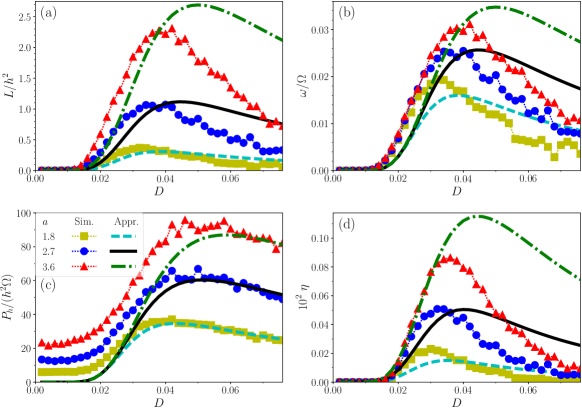
Figure 5: (Color online) (a) $L/h^{2}$, (b) $\omega/\Omega$, (c) $P_{h}/(h^{2}\Omega)$, and (d) $\eta$ versus $D$ under the potentials of parameter family A2 [Fig. 3(b), (d), and (e)].

In parameter family A2, the major and minor radii of the elliptic pathway of the valley are varied as $(a,b)=(1.8,1)$, $(2.7,1.5)$, and $(3.6,2)$ while retaining the similarity. Their corresponding potential landscapes are shown in Fig. 3(b), (d), and (e). With the common parameters $(m,\alpha,\lambda)=(2,0.4\pi,0)$, we set $d$ as in Eq. (81). Thus, $v_{1}(\boldsymbol{x})$ is optimized so that the factor $-\boldsymbol{x}_{+}\cdot\boldsymbol{n}_{+}$ is maximized. Figure 5 shows that the peaks of $L$, $\omega$, $P_{h}$, and $\eta$ increase with the diameter of the elliptic pathway. These are consistent with Eqs. (75)–(80). Here, it should be noted that as the diameter of the pathway increases, the typical magnitude of $V_{h}(\boldsymbol{x},t)$ for $\Delta V$ increases. Then, in order to maintain the local equilibrium condition, it is necessary to decrease $h$ and $\Omega$ with the diameter.

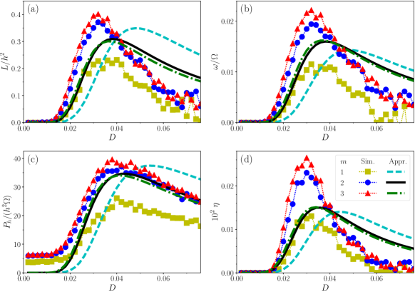
Figure 6: (Color online) (a) $L/h^{2}$, (b) $\omega/\Omega$, (c) $P_{h}/(h^{2}\Omega)$, and (d) $\eta$ versus $D$ under the potentials of parameter family A3 [Fig. 3(b), (f), and (g)].

In parameter family A3, only $m$ is increased as $m\in\{1,2,3\}$. The corresponding potential landscapes are shown in Fig. 3(f), (b), and (g), respectively. In this family, the intersection of the valley narrows for large $m$, whereas the diameters of the pathway are nearly equal. In Fig. 6, we can see that for both numerical and approximation results, each curve of $L$, $\omega$, $P_{h}$, and $\eta$ is likely to approach a certain curve as $m$ increases. The approximation result of $m=1$ deviates exceptionally from such an asymptotic approach. For this reason, we consider that the influence of the external field on the thermal equilibrium condition is relatively large at $m=1$ because of the smaller curvature in the intersection of the valley.

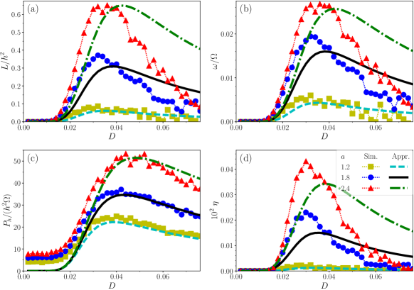
Figure 7: (Color online) (a) $L/h^{2}$, (b) $\omega/\Omega$, (c) $P_{h}/(h^{2}\Omega)$, and (d) $\eta$ versus $D$ under the potentials of parameter family A4 [Fig. 3(b), (h), and (i)].

In parameter family A4, the eccentricity of the elliptic pathway is increased as $\frac{a}{b}=1.2$ [Fig. 3(h)], $1.8$ [(b)], and $2.4$ [(i)]. Each value of $d$ obeys Eq. (81), in which case $-\boldsymbol{x}_{+}\cdot\boldsymbol{n}_{+}$ is maximized. In Fig. 7, we can see that the peaks of $L$, $\omega$, $P_{h}$, and $\eta$ increase with $\frac{a}{b}$. These are consistent with Eqs. (75)–(80). As mentioned previously, for consistency with the local equilibrium condition at larger $\frac{a}{b}$, it is necessary to keep $\Omega$ and $h$ sufficiently small.

We make two remarks about the comparison of the approximation and simulation results. Firstly, our approximation has the adjustable parameters $g_{L}$, $g_{L}^{\prime}$, $g_{O}$, and $g_{V}$ for absorbing complexities in the coarse-grained approach, which we have determined by eye so that the approximations agree as much as possible with all the simulation results. Therefore, rather than focusing on the difference in height between the two results for each individual parameter, it is reasonable to compare them in relation to the similarities among the plotted curves in a parameter family. From this respect, regarding the relationship between the peak heights in Figs. 4–7, the approximation is consistent with the simulation results except for the case of $m=1$ in Fig. 6. As mentioned above, if the local equilibrium condition holds well, our approximation can have such a consistency. Secondly, it can be observed that the agreement between the two results seems better for the lowest curves in Figs. 4 and 7. We consider this to be a visual effect whereby, when observing the upper and lower curves for a couple of parameter sets in a panel in these figures, the difference between the two results for the lower curve is more inconspicuous than that for the upper one.

V.2 Weakly distorted elliptic case ($\lambda\neq 0$)

Label	Key param. vals.		Figs.	$\alpha$ and/or $d$
B1	$d$	$1.9000_{\ast}$	Fig. 8(a)	$\alpha$	$0.4766\pi_{\ast}$
		$2$	Fig. 8(b)		$0.4095\pi$
		$3$	Fig. 1		$0.3392\pi$
B2	$e$	$2$	Fig. 8(c)	$(\alpha,d)$	$(0.4824\pi_{\ast},1.7384_{\ast})$
		$3$	Fig. 8(d)		$(0.4785\pi_{\ast},1.8270_{\ast})$
		$8$	Fig. 8(a)		$(0.4766\pi_{\ast},1.9000_{\ast})$
B3	$\lambda$	$0.1$	Fig. 8(e)	$(\alpha,d)$	$(0.4902\pi_{\ast},1.8335_{\ast})$
		$0.1$			$(0.4249\pi,1.85)$
		$0.27$	Fig. 8(a)		$(0.4766\pi_{\ast},1.9000_{\ast})$
		$1.2$	Fig. 8(f)		$(0.4297\pi_{\ast},2.4091_{\ast})$
B4	$\beta$	$0$	Fig. 8(g)	$(\alpha,d)$	$(0.4639\pi_{\ast},1.8784_{\ast})$
		$0$			$(0.4150\pi,1.9)$
		$0.05\pi$	Fig. 8(a)		$(0.4766\pi_{\ast},1.9000_{\ast})$
		$0.05\pi$			$(0.4238\pi,1.95)$
		$0.15\pi$	Fig. 8(h)		$(0.4980\pi_{\ast},1.8133_{\ast})$

Table 2: List of parameter families in weakly distorted elliptic case. The first and second columns consist of labels and key parameters, respectively. For values of $\alpha$ and $d$ in the sixth column, those with an asterisk “$*$” were determined through $\mathrm{G}_{3}$ [Eq. (82)]; without an asterisk, $d$ is modified as $d=d_{\ast}+\epsilon$ with $\epsilon>0$, and then $\alpha$ is determined through $\mathrm{G}_{2}$. The common parameters for each family are as follows: B1: $(m,a,b,e,f,\lambda,\beta)=(2,1.8,1,8,1,0.27,0.05\pi)$; B2: $(m,a,b,f,\lambda,\beta)=(2,1.8,1,1,0.27,0.05\pi)$; B3: $(m,a,b,e,f,\beta)=(2,1.8,1,8,1,0.05\pi)$; B4: $(m,a,b,e,f,\lambda)=(2,1.8,1,8,1,0.27)$. $\Delta V=0.15$ is maintained by modifying $K$, which is more precise than the elliptic case.

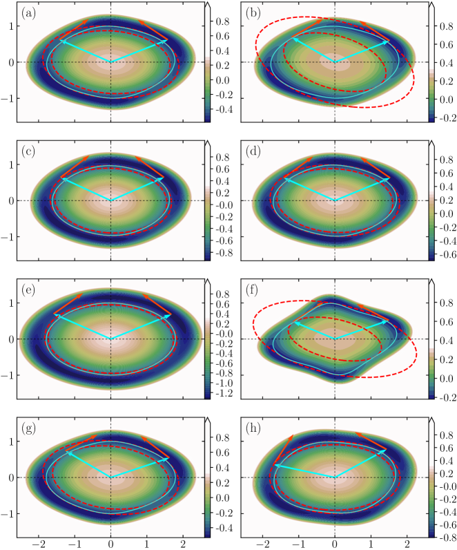
Figure 8: (Color online) Contour graphs of $V_{0}(\boldsymbol{x})$ on $\{\boldsymbol{x}\mid\lvert x\rvert\leq 2.6,\lvert y\rvert\leq 1.664\}$ in the parameter families B1, B2, B3, and B4 in Table 2, and the curves $\mathrm{C}_{\infty}$, $\mathrm{E}_{+}$, and $\mathrm{E}^{+}$. In (a) and (b), $d=d_{\ast}$ and $d_{\ast}+\epsilon$ (B1); in (c) and (d), modulation of the four-fold symmetry ($\frac{e}{f}$) differs (B2); in (e) and (f), $\lambda$ differs (B3); in (g) and (h), $\beta$ differs (B4). See the fourth column in Table 2 for the correspondences.

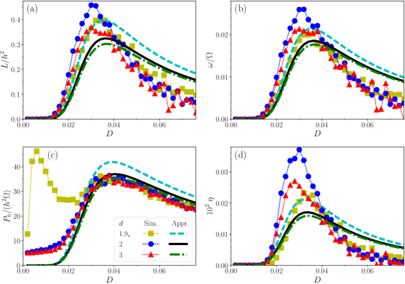
Figure 9: (Color online) (a) $L/h^{2}$, (b) $\omega/\Omega$, (c) $P_{h}/(h^{2}\Omega)$, and (d) $\eta$ versus $D$ under the potentials of parameter family B1 [Figs. 8(a), 8(b), and 1].

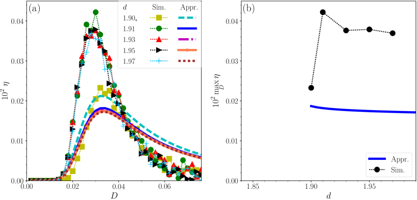
Figure 10: (Color online) (a) $\eta$ versus $D$ for a series of $d$. For each of $d\in\{1.90_{\ast},1.91,1.93,1.95,1.97\}$, retaining $\Delta V=0.15$ and $(m,a,b,e,f,\lambda,\beta)=(2,1.8,1,8,1,0.27,0.05\pi)$, $\alpha$ is optimized via $\mathrm{G}_{2}$; particularly, in the case of $d=1.90_{\ast}$, which being in the parameter family B1 (the first line in Table. 2), $(\alpha,d)$ is optimized via $\mathrm{G}_{3}$. (b) $\displaystyle\max_{D}\eta$ as a function of $d$ for $d\geq 1.90$. As $d$ varies, $\alpha$ is optimized simultaneously via $\mathrm{G}_{2}$ with the other parameters being the same as those in (a). For $1\leq d<1.90$, there is no optimized value of $\alpha$, and the curve is not drawn. The correspondences between the parameters and the types of symbol (numerical simulation results) and curve (approximation results) are shown in the legend boxes.

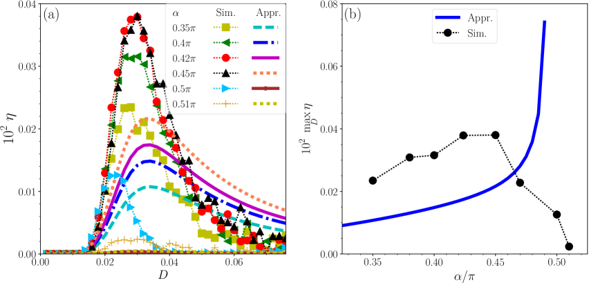
Figure 11: (Color online) (a) $\eta$ versus $D$ for a series of $\alpha$ from $0.35\pi$ to $0.51\pi$. (b) $\displaystyle\max_{D}\eta$ as a function of $\alpha$ over the range treated in (a). While $\alpha$ varies, $d$ is fixed at $1.95$ (i.e., $v_{1}(\boldsymbol{x})$ is not optimized), $\Delta V=0.15$ is retained, and $(m,a,b,e,f,\lambda,\beta)=(2,1.8,1,8,1,0.27,0.05\pi)$.

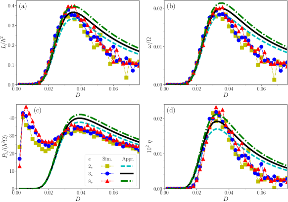
Figure 12: (Color online) (a) $L/h^{2}$, (b) $\omega/\Omega$, (c) $P_{h}/(h^{2}\Omega)$, and (d) $\eta$ versus $D$ under the potentials of parameter family B2 [Fig. 8(c), (d), and (a)].

Outcomes of the optimization described in Sec. IV.2 for $V_{0}(\boldsymbol{x})$ of nonelliptic pathway ($\mathrm{C}_{\infty}$) are shown with the results of the performance indexes according to the parameter families B1–B4 in Table 2. Firstly, let us observe the effect of the relaxation for $d$ in Eq. (84). In parameter family B1, $d$ is varied as $d_{\ast}$, $2$, and $3$, i.e., the first one is determined by $\mathrm{G}_{3}$ [Eq. (82)] together with $\alpha_{\ast}$, and the second and third ones are increased from $d_{\ast}$ in accordance with the moderation procedure [Eq. (84)] followed by readjustment of $\alpha$ through $\mathrm{G}_{2}$. To see the curves $\mathrm{C}_{\infty}$, $\mathrm{E}_{+}$, and $\mathrm{E}^{+}$ in Figs. 8(a), 8(b), and 1, $\mathrm{E}_{+}$ and $\mathrm{E}^{+}$ closely contact to $\mathrm{C}_{\infty}$ for $d=d_{\ast}$ [Fig. 8(a)] and, as $d$ is increased, the space between $\mathrm{E}_{+}$ and $\mathrm{E}^{+}$ becomes wider [Figs. 8(b) and 1].

The simulation results of $L$, $\omega$, and $\eta$ in Fig. 9 demonstrate that the curves of $d=2$ are higher than those of $d=d_{\ast}\approx 1.900$ around the peak region. Turning to the plot of $P_{h}$, the curve of $d=d_{\ast}$ has another peak around $D\approx 0.006$, while the others have only a single peak. A reason for this new peak in $P_{h}$ is, as mentioned in Sec. IV.2, as follows. In the presence of time-dependent fields, instead of the curves $\mathrm{E}_{+}$ and $\mathrm{E}^{+}$, which are defined for $m\rightarrow\infty$ and $h=I=0$, we should consider the temporally moving curves $E^{\ast}(\Phi_{t})$ and $E_{\ast}(\Phi_{t})$ with $v_{1}^{\prime}(\boldsymbol{x},\Phi_{t})$ in Eq. (83). The motion of the circumscribed point of $E_{\ast}(\Phi_{t})$ may temporally create another minimum at a point distant from both $\boldsymbol{x}_{+}$ and $\boldsymbol{x}_{-}$, and then may induce a jump of state. Such a jump motion may expend power associated with a small amount of thermal activation. We can thus relate such a power consumption to the new peak in $P_{h}$. This also suggests that the input power is not applied efficiently to the rotation while employing $v_{1}(\boldsymbol{x})$ such that $\mathrm{E}_{+}$ and $\mathrm{E}^{+}$ enclose $\mathrm{C}_{\infty}$ without sufficient room. In contrast, when making a suitably loose gap between $\mathrm{E}_{+}$ and $\mathrm{E}^{+}$ with $\epsilon$ in Eq. (84), the movement of the minimum can be restricted near either $\boldsymbol{x}_{+}$ or $\boldsymbol{x}_{-}$, in which case the local equilibrium is maintained. We then expect that incorporating the moderation brings a better efficiency. This is consistent with the numerical results for $\eta$ in Fig. 9.

We should also note that the presented approximation cannot predict the extra peak of $P_{h}$. This is because we have assumed that the local equilibrium always holds around the minima of $V_{0}(\boldsymbol{x})$, and have ignored any temporally induced current due to the creation of a temporal minimum. Thus, for the case of $V_{0}(\boldsymbol{x})$ optimized with the moderation, we can assume a local equilibrium, and basically regard the approximation to be consistent with the results of numerical simulation.

We give a more detailed view on the marginal behaviors of $\eta$ in the optimization for $v_{1}(\boldsymbol{x})$ under the procedure $\mathrm{G}_{3}$ followed by the moderation Eq. (84). Figure 10(a) shows the graphs of $\eta$ versus $D$ for a series of $d$ from $1.90$ (the case of $d=1.90_{\ast}\equiv d_{\ast}$ and $\alpha=0.48\pi_{\ast}\equiv\alpha_{\ast}$ in the parameter family B1 in Table 2) to $1.97$, where, for each $d$, $\alpha$ is simultaneously readjusted in accordance with $\mathrm{G}_{2}$, i.e., $\alpha=\displaystyle\operatorname*{arg\,max}_{0\leq\alpha<\frac{\pi}{2}}(-\boldsymbol{x}_{+}\cdot\boldsymbol{n}_{v})$, and $\Delta V=0.15$ is retained by modulating $K$. These curves indicate that the peak is higher as $d$ is closer to $d_{\ast}$, but drops at $d=d_{\ast}$. Figure 10(b) shows the dependence of the peak height on $d$ in the aforementioned settings of parameters. The solid curve thus may approximate $\displaystyle\max_{D,\alpha}\eta$ for $d>d_{\ast}$, whereas it is not defined for $1\leq d<d_{\ast}$, in which no optimized value of $\alpha$ satisfying $\mathrm{G}_{2}$ exists. One can see that the numerical results (symbols) follow the solid curve, except for the difference in their heights. Figure 11 shows (a) the graphs of $\eta$ versus $D$ as only $\alpha$ varies around $\alpha\approx 0.42\pi$ with $d=1.95$, $\Delta V=0.15$ and $(m,a,b,e,f,\lambda,\beta)=(2,1.8,1,8,1,0.27,0.05\pi)$, and (b) $\displaystyle\max_{D}\eta$ over the range of $\alpha$ treated in the panel (a). Recalling that the referenced parameters $\alpha\approx 0.42\pi$ and $d=1.95$ (filled circles or solid curve) are obtained in the moderation procedure for the case of $\alpha_{\ast}>0.42\pi$ and $d_{\ast}$, there is a possibility of raising the peak of $\eta$, i.e., $\displaystyle\max_{D}\eta$, by increasing $\alpha$ from $\alpha\approx 0.42\pi$. However, in the numerical results (symbols), as $\alpha$ is increased, $\displaystyle\max_{D}\eta$ soon plateaus and goes down for $\alpha\geq 0.45\pi$. For $\alpha<0.42\pi$, the peak diminishes monotonically; this implies that $\alpha$ moves away from the optimized point on $d=1.95$. The solid curve for $\displaystyle\max_{D}\eta$ in Fig. 11(b) has a discontinuity at $\alpha\approx 0.49\pi$, where the original two minima of $V_{0}(\boldsymbol{x})$ switch to another two minima (The number of minima of $V_{0}(\boldsymbol{x})$ changes as two, four, and two for $\alpha<0.47\pi$, $0.47\pi\leq\alpha\leq 0.49\pi$, and $0.49\pi<\alpha$, respectively), therefore, the curve is drawn only for the domain lower than the singular point ($\alpha\approx 0.49\pi$). Around that point, it is expected that the local equilibrium assumption breaks, the rotational performance drops as mentioned above, and also our approximation becomes inconsistent with the original assumptions such that the potential always has two minima. Consequently, these results reveal that the moderation procedure works well with a small relaxation parameter.

In parameter family B2, $e$ is increased; with $\frac{e}{f}$ [see Eq. (11)], we can enhance the fourth-order circular harmonic distortion of the shape of the pathway along the potential valley. It is deformed gradually from an ellipse as $\frac{e}{f}$ differs from one. In Fig. 8, we see the shapes of the pathway for $e=2$ (c), $3$ (d), and $8$ (a). In Fig. 12, the approximation curves indicate that the indexes rise as $e$ increases, and the numerical results seem to follow such a tendency, although it is not as clear. The emergence of the peak at $D\approx 0.006$ in $P_{h}$ is, as mentioned above, because of the fact that $(\alpha,d)$ is determined by $\mathrm{G}_{3}$ without the moderation. As in the figure legends, we add an asterisk “$\ast$” to the parameter value(s) for which $(\alpha,d)$ is determined in $\mathrm{G}_{3}$ (see Table 2).

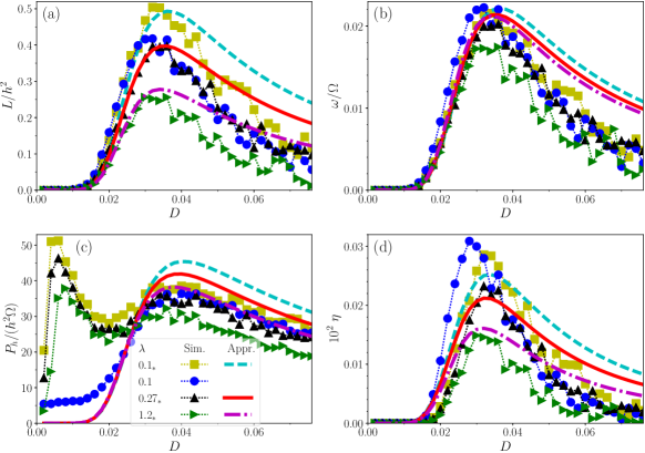
Figure 13: (Color online) (a) $L/h^{2}$, (b) $\omega/\Omega$, (c) $P_{h}/(h^{2}\Omega)$, and (d) $\eta$ versus $D$ under the potentials of parameter family B3 [Fig. 8(e), (a), and (f)].

In parameter family B3, $\lambda$ in Eq. (11) is increased as $0.1$, $0.27$, and $1.2$. As shown in Fig. 8(e), (a), and (f) for $\lambda=0.1$, $0.27$, and $1.2$, the four-fold symmetric modulation on the pathway is conspicuous with $\lambda$. In Fig. 13, we see that the peaks of $L$, $\omega$, $P_{h}$, and $\eta$ decrease with $\lambda$, except for the case $\lambda=0.1$ (filled circles) in which $(\alpha,d)$ is optimized with the modulation. A characteristic of this decrease is that as $\lambda$ is increased, the factor $-\boldsymbol{x}_{+}\cdot\boldsymbol{n}_{+}$ increases; however, the other factor $H_{n}$ increases simultaneously, in which case all the performance indexes decrease.

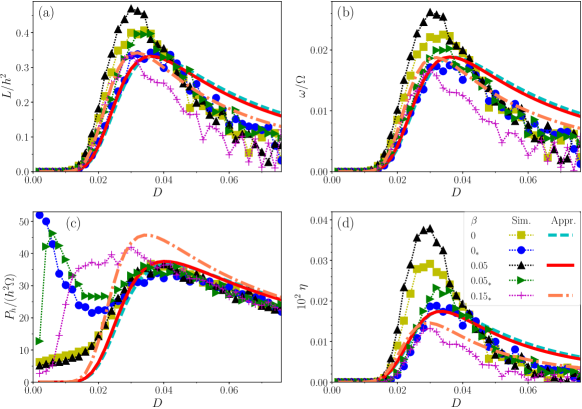
Figure 14: (Color online) (a) $L/h^{2}$, (b) $\omega/\Omega$, (c) $P_{h}/(h^{2}\Omega)$, and (d) $\eta$ versus $D$ under the potentials of parameter family B4 [Fig. 8(g), (a), and (h)].

In parameter family B4, $\beta$ is varied as $\beta=0$, $0.05\pi$, and $0.15\pi$; with $\beta$, the axis of the fourth-order harmonic distortion rotates. In Fig. 8(g), (a), and (h) for $\beta=0$, $0.05\pi$, and $0.15\pi$, respectively, we can see such a rotation. Figure 14 shows that $L$, $\omega$, and $\eta$ have higher peaks for $\beta=0.05\pi$ as $v_{1}(\boldsymbol{x})$ is optimized with the moderation. Finally, let us compare the best result in the elliptic case ($\lambda=0$) in Sec. V.1 with that in the parameter families B1–B4 under the same conditions of $(m,a,b)$ with respect to the peak of $\eta$. For the former, see the case of $(m,a,b)=(2,1.8,1)$, i.e., the curve of $a=1.8$ in Fig. 7 (or that of $m=2$ in Fig. 6 or that of $a=1.8$ in Fig. 5). We can see that $\eta$ for $\beta=0.05\pi$ in Fig. 14 has a higher peak, $\eta\approx 0.038\times 10^{-2}$, than the best one, $\eta\approx 0.023\times 10^{-2}$, in the elliptic case. This result suggests that the term $\lambda$ can contribute to a better efficiency. It also implies that the efficiency could be improved by designing $v_{0}(\boldsymbol{x})$ and $v_{1}(\boldsymbol{x})$ more carefully.

So far, maximizing the performance indexes under the RDDF [Eq. (2)] has been considered by optimizing $V_{0}(\boldsymbol{x})$; however, the value of $\eta$ is very small. Finally, let us discuss the reason for such small efficiency, and a possible way of remodeling to improve it. In the present model, for a small $h$, the field $h\boldsymbol{N}_{t}$ has a role in modulating the ratchet (saw-tooth) profile along the valley by varying the positions of the minima and saddle (or ridge curves) of $V(\boldsymbol{x},t)$ and the slopes around the minima. This eventually causes net rotational motion because of the circular ratchet structure of $V_{0}(\boldsymbol{x})$. However, because the primary action of the field is to cause a linear displacement of the minima and saddles, not all the power of the field is applied to the unidirectional rotational motion; instead, a great deal of the power is scattered to other motions (i.e., rocking motions without bias in the rotational and radial directions) Tutu et al. (2015). Thus, we can conclude that the main reason for the small efficiency lies in the form of the field. The problem of improving the efficiency within the non-biased fields can therefore be recast into a problem of designing the time-dependent part of the potential, $V_{h}(\boldsymbol{x},t)$, or external fields to maximize its power conversion efficiency. Exploiting an idea from one-dimensional ratchet models that incorporate a mechanism for avoiding such a rocking motion with saw-tooth type potentials that are shifted randomly back or forth by an appropriate distance Chauwin et al. (1994); Parmeggiani et al. (1999); Makhnovskii et al. (2004), we may consider a form of the field as $\boldsymbol{f}_{h}(\boldsymbol{x},t)=hq(\boldsymbol{x},t)\partial_{\boldsymbol{x}}\theta(\boldsymbol{x})$. This represents a circular field around the origin, the direction of which varies randomly with the spatial dependency of $q(\boldsymbol{x},t)$. We expect that this can reduce the rocking motion in the radial direction, and may also suppress such diffusive motion in the rotational direction if we appropriately design the spatial and temporal variations of $q(\boldsymbol{x},t)$ in accordance with $V_{0}(\boldsymbol{x})$ imposing a constraint that the spatial average of $\boldsymbol{f}_{h}(\boldsymbol{x},t)$ has no bias.

VI Direction For Three-tooth Ratchet Model

So far, we have dealt with optimizing the two-tooth ratchet potential in Eqs. (10)–(12). However, our approach could be applied to more general ratchet potentials. Here, we show how a similar approach holds for a three-tooth ratchet potential of the same form as $V_{0}(\boldsymbol{x})$ in Eq. (10).

It is necessary that $v_{0}(\boldsymbol{x})$ and $v_{1}(\boldsymbol{x})$ have three-fold symmetry. For $m\gg 1$, the curve $\mathrm{C}_{\infty}:\{\boldsymbol{x}|v_{0}(\boldsymbol{x})=1\}$ corresponds to a potential valley, and the region of $v_{0}(\boldsymbol{x})<1$ must be a simply connected space. Therefore, a simple expression is proposed as

$$v_{0}(\boldsymbol{x})\equiv\lvert\boldsymbol{x}\rvert^{2}+a\lvert\boldsymbol{x}\rvert^{4}+b(\boldsymbol{e}_{0}\cdot\boldsymbol{x})(\hat{g}_{1}\boldsymbol{e}_{0}\cdot\boldsymbol{x})(\hat{g}_{2}\boldsymbol{e}_{0}\cdot\boldsymbol{x}),$$ (85)

where $a$ is positive, so that we have $v_{0}(\boldsymbol{x})\rightarrow\infty$ for $\lvert\boldsymbol{x}\rvert\rightarrow\infty$, and $\lvert b\rvert$ is sufficiently small for such $\mathrm{C}_{\infty}$ of a simply connected curve. Term $\hat{g}_{1}$ ($\hat{g}_{2}$) represents a matrix for a rotation of angle $+\frac{2\pi}{3}$ ($-\frac{2\pi}{3}$):

$$\hat{g}_{1}\equiv\frac{1}{2}\begin{pmatrix}-1&-\sqrt{3}\\ \sqrt{3}&-1\end{pmatrix},\quad\hat{g}_{2}\equiv\frac{1}{2}\begin{pmatrix}-1&\sqrt{3}\\ -\sqrt{3}&-1\end{pmatrix}.$$ (86)

The third term adds a third circular harmonic in $\mathrm{C}_{\infty}$; $\boldsymbol{e}_{0}$ is a reference axis on the azimuthal angle about the origin. Note that as $\boldsymbol{e}_{0}$ rotates, $\mathrm{C}_{\infty}$ rotates by the same angle about the origin. Without loss of generality, we have $b>0$ and $\boldsymbol{e}_{0}=(1,0)^{\mathrm{T}}$. Similarly, $v_{1}(\boldsymbol{x})$ is given as

$$v_{1}(\boldsymbol{x})\equiv\lvert\boldsymbol{x}\rvert^{2}+c\lvert\boldsymbol{x}\rvert^{4}+d(\boldsymbol{e}_{1}\cdot\boldsymbol{x})(\hat{g}_{1}\boldsymbol{e}_{1}\cdot\boldsymbol{x})(\hat{g}_{2}\boldsymbol{e}_{1}\cdot\boldsymbol{x})$$ (87)

with a reference axis $\boldsymbol{e}_{1}\equiv(\cos\alpha,\sin\alpha)^{\mathrm{T}}$ and positive values $c$ and $d$.

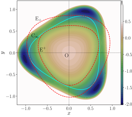
Figure 15: (Color online) Contour plot of a three-tooth ratchet potential with skeletons of $\mathrm{C}_{\infty}:\{v_{0}(\boldsymbol{x})=1\}$, $\mathrm{E}_{+}$, and $\mathrm{E}^{+}$. The parameters of $V_{0}(\boldsymbol{x})$ of Eqs. (10), (85)–(87) are $(m,a,b,c,d,K,\alpha)=(2,1,3,1,2,1,0.52\pi)$. $\mathrm{E}_{+}$ and $\mathrm{E}^{+}$ correspond to the curves $\{v_{1}(\boldsymbol{x})=E\}$ for $E=1.62$ (externally tangent case) and $0.67$ (internally tangent case), respectively.

Figure 15 shows a contour graph of the three-tooth ratchet potential of Eqs. (10), (85)–(87). The curves $\mathrm{E}_{+}$ and $\mathrm{E}^{+}$ on the graph represent the circumscribed and inscribed curves of $\mathrm{E}:\{\boldsymbol{x}\mid v_{1}(\boldsymbol{x})=E\}$ to $\mathrm{C}_{\infty}$ with $E=1.62$ and $0.67$, respectively. The externally (internally) tangent points correspond to the local minima (saddles) of $V_{0}(\boldsymbol{x})$. For $m\rightarrow\infty$, these minima and saddles satisfy Eq. (17).

The optimization of $L$, $\omega$, and $\eta$ can be carried out through the maximization of a factor such as $I_{0}(D)$ [Eq. (65)], which can be obtained by following the procedure in Appendix D. Similarly, let us assume that the factor $-\boldsymbol{x}_{\ast}\cdot\boldsymbol{n}(\boldsymbol{x}_{\ast})$ at a local minimum point $\boldsymbol{x}_{\ast}$ affects the maximization of $I_{0}(D)$ more than it does $H_{n}$. We then employ the strategy to maximize $-\boldsymbol{x}\cdot\boldsymbol{n}_{v}(\boldsymbol{x})$ using $v_{0}(\boldsymbol{x})$ and $v_{1}(\boldsymbol{x})$ with the assumption that $m\gg 1$. In particular, letting $p$ be a target parameter in $v_{1}(\boldsymbol{x})$ for the optimization, the problem is to solve Eqs. (68) and (69); the actual procedure follows Eq. (71) in Sec. IV.1 as

$$\boldsymbol{x}_{\ast}=\operatorname*{arg\,max}_{\boldsymbol{x}\in\mathrm{C}_{\infty}}\left\{-\boldsymbol{x}\cdot\boldsymbol{n}_{v}(\boldsymbol{x})\right\},$$ (88)

and then, with this $\boldsymbol{x}_{\ast}$, we find such $p$ as satisfies Eqs. (17) and (69) [replace $\boldsymbol{x}_{\ast}$ with $\boldsymbol{x}_{+}$].

As described in Sec. IV.2, if we choose $v_{1}(\boldsymbol{x})$ to be a different functional form from $v_{0}(\boldsymbol{x})$, we can further arrange the values of target parameters in $v_{1}(\boldsymbol{x})$ to decrease $g(\boldsymbol{x})$ within a suitable range. For example, we can consider a $v_{0}(\boldsymbol{x})$ that has the sixth circular harmonic deformation. In such a case, as in Sec. IV.2, letting $\alpha$ and $d$ in $v_{1}(\boldsymbol{x})$ be target parameters, we first determine $\alpha_{\ast}$ and $d_{\ast}$ as

$$(\alpha_{\ast},d_{\ast})=\operatorname*{arg\,min}_{0\leq\alpha<\frac{\pi}{3},d(\alpha)}E_{+},$$ (89)

where $d(\alpha)$ means a function that relates $\alpha$ to $d$ through Eq. (17). Next, to prevent the creation of temporal minima, we moderate the above minimization by replacing $d$ with $d=d_{\ast}+\epsilon$ ($\epsilon>0$), and revise $\alpha$ to satisfy Eq. (17) with this $d$. We expect this procedure to bring about a robust local equilibrium for external fields and to reduce the power consumption for rotation. By observing the numerical result for $P_{h}$, we can confirm whether the local equilibrium has been retained.

VII Summary

The underlying themes in this study have been to elucidate the types of ratchet model (as combinations of the 2D ratchet potential and the unbiased randomly varying field) that produce a robust net rotation, and to determine how to maximize the rotational output and efficiency. In this paper, we have shown that the proposed ratchet model, consisting of a 2D two-tooth ratchet potential and an RDDF, generates a net rotation in the direction of the ratchet potential, i.e., the chirality. The 2D three-tooth ratchet model also possesses such a property Tutu and Nagata (2013); Tutu et al. (2015).

The mechanism of net rotation is not so obvious because the deformation along the valley in the 2D ratchet model can be composed of various types of deformation. The mathematical origin of the net rotation can be found in Eq. (124), i.e., $L,\omega\propto\overline{\ln\left[\frac{P(\mu,t)P(-\mu,t)}{Q(\mu,t)^{2}}\right]J^{\mu}(t)}$, in which $J^{\mu}(t)$, the barrier-crossing current, and the multiplied factor, the entropy-like measure for the deviation of the positional distribution from the equilibrium one, are correlated as a result of the rectification effect due to the chirality, and the average of these products remains a bias [Eq. (126)].

Another explanation uses a ratchet exposed to an external field made of superimposed uni-axially polarized fields within the same 2D plane. The mechanism for the net rotation of a two-tooth ratchet under a uni-axially polarized randomly varying field can be explained using the mechanism for the propeller rotation of a “gee-haw whammy diddle” or “propeller stick” Wikipedia (2016) (cf. Tutu and Hoshino (2011)). Employing $M$ copies of such a uni-axially polarized field, we orient their angles of polarization to $\phi_{k}=\frac{2\pi k}{M}$ ($0\leq k<M$), respectively, whereby the ratchet is exposed to the field $\sum_{k}h_{k}(t)\boldsymbol{N}_{k}$ (cf. Eq. (2)), where $\boldsymbol{N}_{k}=(\cos\phi_{k},\sin\phi_{k})$ and $h_{k}(t)$ is a unbiased dichotomic noise, independent of the others and varying between $-\frac{h}{\sqrt{M}}$ and $\frac{h}{\sqrt{M}}$ with mean frequency $\Omega$. Thus, this field mimics the RDDF. Then, as a total of the propeller-stick-like responses to the individual fields, we can expect this ratchet to yield a net rotation in the direction determined by its chirality.

The optimization of the 2D ratchet potential has been considered by employing the redesigned form of the ratchet potential in Eq. (10). In the proposed potential, the parameter $m$ controls the sharpness of the valley; thereby, for $m\gg 1$, the two curves with $\mathrm{C}_{\infty}:\{\boldsymbol{x}\mid v_{0}(\boldsymbol{x})=1\}$ and $\mathrm{E}:\{\boldsymbol{x}\mid v_{1}(\boldsymbol{x})=E\}$ determine a skeleton of the 2D ratchet potential, and the eigenvalues of the Hessian matrix are expressed approximately in terms of the quantities derived from $\mathrm{C}_{\infty}$ and $\mathrm{E}$ (Sec. II). These enable us to easily design a strategy for maximizing the performance indexes [$L$ (MAM), $\omega$ (MAV), and $\eta$ (efficiency)].

From the analytic expressions for $L$ and $\omega$ (Secs. III.3), we have specified the factor $-\boldsymbol{x}_{+}\cdot\boldsymbol{n}_{+}$ as the main objective function to maximize, and $H_{n}$ as the optional one to minimize within the appropriate range for the local equilibrium condition. Quantities $-\boldsymbol{x}_{+}\cdot\boldsymbol{n}_{+}$ and $H_{n}$ are relevant to the asymmetry of the potential profile along the pathway and the curvature at the potential minimum, respectively. Through the optimization of $v_{1}(\boldsymbol{x})$, the procedure to maximize the main factor $-\boldsymbol{x}_{+}\cdot\boldsymbol{n}_{+}$ consists of $\mathrm{G}_{1}$ [Eq. (71)] and $\mathrm{G}_{2}$ [Eq. (72)] (Sec. IV.1), and the one to minimize $H_{n}$ consists of $\mathrm{G}_{3}$ [Eq. (82)] and its moderation [Eq. (84)] (Sec. IV.2). The moderation of $\mathrm{G}_{3}$ is required to prevent the creation of temporal minima. We reason that such temporal minima cause extra dissipation that is observed as another peak in $P_{h}$; the relaxation parameter $\epsilon$ [Eq. (84)] is determined so that $P_{h}$ has no additional peak in the plot for the noise intensity $D$. Although the proposed optimization method has been implemented on the basis of the two-tooth ratchet model, it is applicable to three-tooth or other similar ratchet models (Sec. VI) if $\mathrm{G}_{2}$ is generalized as in Eq. (17).

The outcomes of the optimization have been shown in Secs. IV.1.1 and V for the cases of $\mathrm{C}_{\infty}$ given by elliptic or nonelliptic curves. The analytical expressions for the maximized $L$, $\omega$, and $\eta$ are shown in the elliptic case (Secs. IV.1.1 and D). Consistent with the numerical simulation results in Sec. V.1, these suggest that the peaks of $L$, $\omega$, and $\eta$ increase as the diameter or eccentricity of the ellipse becomes larger. A note for applying such larger values of diameter or eccentricity is that $h$ and $\Omega$ must be sufficiently small to retain the local equilibrium. In the nonelliptic case (Sec. IV.2), the optimization procedure $\mathrm{G}_{3}$ with the moderation is useful; compared with no moderation, it improves the efficiency with a suitable choice of the relaxation parameter. In comparing the efficiency between the elliptic ($\lambda=0$) and nonelliptic ($\lambda\neq 0$) cases under the same condition of $(m,a,b)$, we have seen that the best result in the latter case exhibits a higher peak than the best one in the former. This suggests that a more sophisticated design of $v_{0}(\boldsymbol{x})$, incorporating higher-order harmonic deformations, could improve efficiency.

Appendix A correlation matrix of randomly directed force

We consider the time correlation matrix for $\boldsymbol{N}_{t}=(\cos\Phi_{t},\sin\Phi_{t})^{\mathrm{T}}$, which changes its direction randomly at the rate $\Omega$ independent of the current direction. The angle $\Phi_{t}\in[0,2\pi)$ is a stationary Markov jump process, whose conditional probability density for the transition from $\Phi_{t}=\phi^{\prime}$ during an infinitesimal interval $\Delta t>0$ obeys $p_{\Phi}(\phi,t+\Delta t\mid\phi^{\prime},t)=(1-\Delta t\Omega)\delta(\phi-\phi^{\prime})+\Delta t\Omega p_{\Phi}(\phi)+o(\Delta t)$ with non-negative $p_{\Phi}(\phi)$ satisfying $\int_{0}^{2\pi}p_{\Phi}(\phi)d\phi=1$ and the Dirac’s delta function $\delta(\cdot)$. This leads to the master equation for $p_{\Phi}(\phi,t\mid\phi^{\prime},t^{\prime})$ ($t\geq t^{\prime}$) as

$$\partial_{t}p_{\Phi}(\phi,t\mid\phi^{\prime},t^{\prime})=-\Omega p_{\Phi}(\phi,t\mid\phi^{\prime},t^{\prime})+\Omega p_{\Phi}(\phi).$$ (90)

It is obvious that the stationary probability density of $\Phi_{t}$ coincides with $p_{\Phi}(\phi)$.

The master equation is solved as

$$p_{\Phi}(\phi,t\mid\phi^{\prime},t^{\prime})=p_{\Phi}(\phi)+e^{-\Omega(t-t^{\prime})}\left\{\delta(\phi-\phi^{\prime})-p_{\Phi}(\phi)\right\}.$$ (91)

For $A_{t}\equiv A(\Phi_{t})$ and $B_{t}\equiv B(\Phi_{t})$, where $A(\phi)$ and $B(\phi)$ are any functions of $\phi$, the statistical average of $A_{t}B_{0}$ ($t\geq 0$) with respect to $\{\Phi_{t}\}$ reads as

$$\left\langle A_{t}B_{0}\right\rangle_{\Phi} =\int_{0}^{2\pi}d\phi\int_{0}^{2\pi}d\phi^{\prime}A(\phi)B(\phi^{\prime})p_{\Phi}(\phi,t\mid\phi^{\prime},0)p_{\Phi}(\phi^{\prime})$$

$$=\int_{0}^{2\pi}d\phi\int_{0}^{2\pi}d\phi^{\prime}A(\phi)B(\phi^{\prime})\left[p_{\Phi}(\phi)+e^{-\Omega t}\left\{\delta(\phi-\phi^{\prime})-p_{\Phi}(\phi)\right\}\right]p_{\Phi}(\phi^{\prime})$$

$$=(1-e^{-\Omega t})\langle A_{0}\rangle_{\Phi}\langle B_{0}\rangle_{\Phi}+\langle A_{0}B_{0}\rangle_{\Phi}e^{-\Omega t},$$ (92)

which leads to the time correlation function for $t\geq 0$:

$$\left\langle A_{t}B_{0}\right\rangle_{\Phi}-\langle A_{0}\rangle_{\Phi}\langle B_{0}\rangle_{\Phi}=e^{-\Omega t}\{\langle A_{0}B_{0}\rangle_{\Phi}-\langle A_{0}\rangle_{\Phi}\langle B_{0}\rangle_{\Phi}\}.$$ (93)

The rotational symmetry for $\boldsymbol{N}_{t}$, i.e., $p_{\Phi}(\phi)=\frac{1}{2\pi}$, is further assumed in the paper, which leads to $\left\langle\cos\Phi_{0}\sin\Phi_{0}\right\rangle_{\Phi}=\left\langle\sin\Phi_{0}\cos\Phi_{0}\right\rangle_{\Phi}=0$ and $\left\langle\cos\Phi_{0}\cos\Phi_{0}\right\rangle_{\Phi}=\left\langle\sin\Phi_{0}\sin\Phi_{0}\right\rangle_{\Phi}=1/2$, and thus, by Eq. (93), $\left\langle\boldsymbol{N}_{t}\boldsymbol{N}_{0}^{\mathrm{T}}\right\rangle_{\Phi}=(e^{-\Omega t}/2)\hat{1}$ (Eq. (3)).

Appendix B Transition Rates

The transition rate $W(\sigma,\mu,t)$ [$\sigma,\mu\in\{+,-\}$] in Eq. (51) is derived based on Langer’s method Langer (1968); Hänggi et al. (1990). Let $\tilde{\mathrm{B}}_{\epsilon}^{\mu}$ be a narrow band region with thickness $2\epsilon$ inside which the ridge curve $\tilde{\mathrm{B}}^{\mu}$ is contained (see Fig. 2, or Fig. 6 in Tutu et al. (2015)). In the regions $\tilde{\mathrm{B}}_{\epsilon}^{\mu}$, the current density $\boldsymbol{J}(\boldsymbol{x},t)$ is concentrated by bottleneck structures, whereas, in the central region of $\mathrm{D}_{\epsilon}^{\mu}$, $\boldsymbol{J}(\boldsymbol{x},t)$ can be regarded approximately as vanishing. Thus, we may specify locally non-equilibrium or equilibrium regions either inside or outside $\tilde{\mathrm{B}}_{\epsilon}^{\mu}$. On each region, we assume $\boldsymbol{J}(\boldsymbol{x},t)$ as follows Tutu et al. (2015).

1. In the domain $\mathrm{D}_{\sigma}^{\mu}$ complementary to $\tilde{\mathrm{B}}_{\epsilon}^{\mu}$, i.e., $\mathrm{D}_{\sigma}^{\mu}\setminus\tilde{\mathrm{B}}_{\epsilon}^{\mu}$, we assume $\boldsymbol{J}(\boldsymbol{x},t)\approx\boldsymbol{0}$, i.e., $p(\boldsymbol{x},t)$ approximately obeys the thermal equilibrium probability density function. Then, we have $p(\boldsymbol{x},t)\approx e^{-V(\boldsymbol{x},t)/D}e^{V(\boldsymbol{y},t)/D}p(\boldsymbol{y},t)$ for $\boldsymbol{x},\boldsymbol{y}\in\mathrm{D}_{\sigma}^{\mu}\setminus\tilde{\mathrm{B}}_{\epsilon}^{\mu}$. From Eq. (39), this leads to

   $$P(\sigma,\mu,t)\approx\int_{\boldsymbol{x}\in\mathrm{D}_{\sigma}^{\mu}}d\boldsymbol{x}\,e^{-V(\boldsymbol{x},t)/D}e^{V(\boldsymbol{y},t)/D}p(\boldsymbol{y},t),$$ (94)

   where we assume $p(\boldsymbol{x},t)\approx 0$ for $\boldsymbol{x}\in\tilde{\mathrm{B}}_{\epsilon}^{\mu}$. Also, we have

   $$P(\sigma,t)\approx\int_{\boldsymbol{x}\in\mathrm{D}_{\sigma}}d\boldsymbol{x}\,e^{-V(\boldsymbol{x},t)/D}e^{V(\boldsymbol{y},t)/D}p(\boldsymbol{y},t).$$ (95)

2. Consider a family of curves that are parallel to the curve $\tilde{\mathrm{B}}^{\mu}$ in $\tilde{\mathrm{B}}_{\epsilon}^{\mu}$, and unit vectors $\tilde{\boldsymbol{\tau}}_{\sigma}^{\mu}(\boldsymbol{x})$ and $\tilde{\boldsymbol{n}}_{\sigma}^{\mu}(\boldsymbol{x})$ that are tangent and normal, respectively, to such a curve passing through a point $\boldsymbol{x}\in\tilde{\mathrm{B}}_{\epsilon}^{\mu}$. Then, we assume that a current can arise along the vector field $\tilde{\boldsymbol{n}}_{\sigma}^{\mu}(\boldsymbol{x})$, while an equilibrium condition is retained along the direction $\tilde{\boldsymbol{\tau}}_{\sigma}^{\mu}(\boldsymbol{x})$. Namely, we have $\tilde{\boldsymbol{\tau}}_{\sigma}^{\mu}(\boldsymbol{x})\cdot\boldsymbol{J}(\boldsymbol{x},t)=0$ and $\tilde{J}_{\mu}\equiv\tilde{\boldsymbol{n}}_{\sigma}^{\mu}(\boldsymbol{x})\cdot\boldsymbol{J}(\boldsymbol{x},t)$ in which $\tilde{J}_{\mu}$ is a constant on a curve perpendicularly crossing the family of the curves parallel to $\tilde{\mathrm{B}}^{\mu}$ ($\tilde{J}_{\mu}$ depends on the coordinate on $\tilde{\mathrm{B}}^{\mu}$). Therefore, $J^{\mu}(t)$ in Eq. (43) reads as

   $$J^{\mu}(t)\approx\left(\delta_{\sigma,-\mu}-\delta_{\sigma,\mu}\right)\int_{\boldsymbol{x}\in\tilde{\mathrm{B}}^{\mu}}d\boldsymbol{x}\,\tilde{J}_{\mu}.$$ (96)

To estimate the integration in Eq. (94), let us define a local coordinate system $\boldsymbol{x}=\boldsymbol{x}_{\sigma}+\sigma\mu(\xi\boldsymbol{\tau}_{\sigma}+\eta\boldsymbol{n}_{\sigma})$ near $\boldsymbol{x}_{\sigma}$ with the unit tangential and normal vectors to $\mathrm{B}_{\sigma}$, $\boldsymbol{\tau}_{\sigma}$, and $\boldsymbol{n}_{\sigma}$, at $\boldsymbol{x}=\boldsymbol{x}_{\sigma}$, as eigenvectors of $\hat{G}(\boldsymbol{x}_{\sigma})=\partial_{\boldsymbol{x}}\partial_{\boldsymbol{x}}^{\mathrm{T}}V(\boldsymbol{x}_{\sigma},t)$. Here, the values of $\sigma$ and $\mu$, “$+$” and “$-$”, are mapped to the numbers $+1$ and $-1$, respectively. Then, we expand $V(\boldsymbol{x},t)$ as

$$V(\boldsymbol{x},t)\approx V(\boldsymbol{x}_{\sigma},t)-\mu\boldsymbol{f}_{\sigma}\cdot\left(\xi\boldsymbol{\tau}_{+}+\eta\boldsymbol{n}_{+}\right)+\frac{1}{2}\Lambda_{\tau}(\boldsymbol{x}_{\sigma})\xi^{2}+\frac{1}{2}\Lambda_{n}(\boldsymbol{x}_{\sigma})\eta^{2},$$ (97)

where $\boldsymbol{f}_{\sigma}\equiv\boldsymbol{f}_{I}(\boldsymbol{x}_{\sigma})+h\boldsymbol{N}_{t}$. Note that the eigenvalues of $\hat{G}(\boldsymbol{x}_{\sigma})$, $\Lambda_{\tau}(\boldsymbol{x}_{\sigma})$, and $\Lambda_{n}(\boldsymbol{x}_{\sigma})$ depend on $I$. Since $h$ and $D$ are assumed to be small, neglecting the terms of $O(h^{2})$, we estimate the integration in Eq. (94) as

$$\int_{\boldsymbol{x}\in\mathrm{D}_{\sigma}^{\mu}}d\boldsymbol{x}e^{-\frac{V(\boldsymbol{x},t)}{D}} \approx e^{-\frac{V(\boldsymbol{x}_{\sigma},t)}{D}}\int_{0}^{\infty}d\eta\int_{-\infty}^{\infty}d\xi e^{-\frac{\Lambda_{\tau}(\boldsymbol{x}_{\sigma})\xi^{2}+\Lambda_{n}(\boldsymbol{x}_{\sigma})\eta^{2}}{2D}}\left(1+\frac{\mu\boldsymbol{f}_{\sigma}\cdot\boldsymbol{n}_{+}}{D}\eta\right)$$

$$\approx\frac{e^{-\frac{V(\boldsymbol{x}_{\sigma},t)}{D}}}{2}\sqrt{\frac{2\pi D}{\Lambda_{\tau}(\boldsymbol{x}_{\sigma})}}\left(\sqrt{\frac{2\pi D}{\Lambda_{n}(\boldsymbol{x}_{\sigma})}}+\frac{2\mu\boldsymbol{f}_{\sigma}\cdot\boldsymbol{n}_{+}}{\Lambda_{n}(\boldsymbol{x}_{\sigma})}\right),$$ (98)

where we have used the Gaussian integral approximation by the replacement $\int_{\boldsymbol{x}\in\mathrm{D}_{\sigma}^{\mu}}d\boldsymbol{x}\rightarrow\int_{-\infty}^{\infty}\int_{0}^{\infty}d\xi d\eta$.

Substituting Eq. (98) to Eqs. (94) and (95), we obtain

$$P(\sigma,t)\approx\frac{2\pi D}{\sqrt{\Lambda_{\tau}(\boldsymbol{x}_{\sigma})\Lambda_{n}(\boldsymbol{x}_{\sigma})}}e^{-V(\boldsymbol{x}_{\sigma},t)/D}e^{V(\boldsymbol{y},t)/D}p(\boldsymbol{y},t),$$ (99)

$$P(\sigma,\mu,t)\approx Q(\mu\mid\sigma,t)P(\sigma,t),$$ (100)

$$Q(\mu\mid\sigma,t)\approx\frac{1}{2}\left(1+\frac{2\mu\boldsymbol{f}_{\sigma}\cdot\boldsymbol{n}_{+}}{\sqrt{2\pi D\Lambda_{n}(\boldsymbol{x}_{\sigma})}}\right).$$ (101)

Similarly, on the local coordinate system near $\tilde{\boldsymbol{x}}^{\mu}\in\tilde{\mathrm{B}}^{\mu}$, $\boldsymbol{x}=\tilde{\boldsymbol{x}}^{\mu}+\xi\tilde{\boldsymbol{\tau}}^{\mu}_{\sigma}+\eta\tilde{\boldsymbol{n}}^{\mu}_{\sigma}$, where $\tilde{\boldsymbol{\tau}}_{\sigma}^{\mu}\equiv\tilde{\boldsymbol{\tau}}_{\sigma}^{\mu}(\tilde{\boldsymbol{x}}^{\mu})$ and $\tilde{\boldsymbol{n}}_{\sigma}^{\mu}\equiv\tilde{\boldsymbol{n}}_{\sigma}^{\mu}(\tilde{\boldsymbol{x}}^{\mu})$ (see Sec. III.1), we expand $V(\boldsymbol{x},t)$ as

$$V(\boldsymbol{x},t)\approx V(\tilde{\boldsymbol{x}}^{\mu},t)+V_{\tau}(\xi,t)+V_{n}(\eta,t),$$ (102)

$$V_{\tau}(\xi,t)\equiv\frac{1}{2}\Lambda_{\tau}(\tilde{\boldsymbol{x}}^{\mu})\xi^{2},\quad V_{n}(\eta,t)\equiv\frac{1}{2}\Lambda_{n}(\tilde{\boldsymbol{x}}^{\mu})\eta^{2}.$$ (103)

Because $\tilde{\boldsymbol{\tau}}_{\sigma}^{\mu}\cdot\boldsymbol{J}(\boldsymbol{x},t)=0$, or

$$0=\left[-\partial_{\xi}V(\boldsymbol{x},t)\right]p(\boldsymbol{x},t)-D\partial_{\xi}p(\boldsymbol{x},t),$$ (104)

then by separation of variables, we have $p(\boldsymbol{x},t)\equiv\exp\left[-\frac{V_{\tau}(\xi,t)}{D}\right]p_{n}(\eta,t)$ for $\boldsymbol{x}\in\tilde{\mathrm{B}}_{\epsilon}^{\mu}$.

Multiplying $\tilde{J}_{\mu}=\tilde{\boldsymbol{n}}_{\sigma}^{\mu}(\boldsymbol{x})\cdot\boldsymbol{J}(\boldsymbol{x},t)$ by $e^{V_{n}(\eta,t)/D}$, and integrating over $\eta$ in the range $[-\epsilon,\epsilon]$, we obtain

$$\int_{-\epsilon}^{\epsilon}d\eta\,e^{V_{n}(\eta,t)/D}\tilde{J}_{\mu}=\int_{-\epsilon}^{\epsilon}d\eta\,e^{V_{n}(\eta,t)/D}\left\{\left[-\partial_{\eta}V(\boldsymbol{x},t)\right]p(\boldsymbol{x},t)-D\partial_{\eta}p(\boldsymbol{x},t)\right\}.$$ (105)

From the assumption for $\tilde{J}_{\mu}$, this leads to

$$\tilde{J}_{\mu}=\frac{D}{\int_{-\epsilon}^{\epsilon}dy\,e^{V_{n}(y,t)/D}}\left.\exp\left[\frac{-V_{\tau}(\xi,t)+V_{n}(\eta,t)}{D}\right]p_{n}(\eta,t)\right\rvert_{\eta=\epsilon}^{\eta=-\epsilon}.$$ (106)

From Eq. (99), we have

$$e^{V(\boldsymbol{y},t)/D}p(\boldsymbol{y},t)\bigr{\rvert}_{\boldsymbol{y}=\tilde{\boldsymbol{x}}^{\mu}+\epsilon\mu\tilde{\boldsymbol{n}}_{\sigma}} \approx\frac{\sqrt{\Lambda_{\tau}(\boldsymbol{x}_{\mu\sigma})\Lambda_{n}(\boldsymbol{x}_{\mu\sigma})}}{2\pi De^{-V(\boldsymbol{x}_{\mu\sigma},t)/D}}P(\mu\sigma,t).$$ (107)

Applying this to $e^{V_{n}(\eta,t)/D}p_{n}(\eta,t)\bigr{\rvert}_{\eta=\epsilon}^{\eta=-\epsilon}=e^{\{V(\boldsymbol{y},t)-V(\tilde{\boldsymbol{x}}^{\mu},t)\}/D}p(\boldsymbol{y},t)\bigr{\rvert}_{\boldsymbol{y}=\tilde{\boldsymbol{x}}^{\mu}+\epsilon\mu\tilde{\boldsymbol{n}}_{\sigma}}^{\boldsymbol{y}=\tilde{\boldsymbol{x}}^{\mu}-\epsilon\mu\tilde{\boldsymbol{n}}_{\sigma}}$ in Eq. (106), we obtain

$$\tilde{J}^{\mu}=W_{\xi}(\sigma,\mu,t)P(-\sigma,t)-W_{\xi}(-\sigma,\mu,t)P(\sigma,t)$$ (108)

with

$$W_{\xi}(\sigma,\mu,t)\equiv\frac{1}{2\pi}\frac{\sqrt{\Lambda_{\tau}(\boldsymbol{x}_{-\sigma})\Lambda_{n}(\boldsymbol{x}_{-\sigma})}}{\int_{-\epsilon}^{\epsilon}dy\,e^{V_{n}(y,t)/D}}\exp\left\{\frac{V(\boldsymbol{x}_{-\sigma},t)-V_{\tau}(\xi,t)-V(\tilde{\boldsymbol{x}}^{\mu},t)}{D}\right\}.$$ (109)

From Eqs. (96) and (109), the transition rate $W(\sigma,\mu,t)$ in Eq. (50) is found to be

$$W(\sigma,\mu,t)\approx\frac{1}{2\pi}e^{-\left[V(\boldsymbol{x}^{\mu},t)-V(\boldsymbol{x}_{-\sigma},t)\right]/D}\sqrt{\frac{\Lambda_{\tau}(\boldsymbol{x}_{-\sigma})\Lambda_{n}(\boldsymbol{x}_{-\sigma})\lvert\Lambda_{n}(\tilde{\boldsymbol{x}}^{\mu})\rvert}{\Lambda_{\tau}(\tilde{\boldsymbol{x}}^{\mu})}}.$$ (110)

Here, we have approximated $\int_{-\epsilon}^{\epsilon}dy\,e^{V_{n}(y,t)/D}$ and $\int_{\boldsymbol{x}\in\mathrm{B}^{\mu}}d\xi\,e^{-V_{\tau}(\xi,t)/D}$ with the Gaussian integrals $\int_{-\infty}^{\infty}d\eta\,e^{\Lambda_{n}(\tilde{\boldsymbol{x}}^{\mu})\eta^{2}/(2D)}=\sqrt{\frac{2\pi D}{\lvert\Lambda_{n}(\tilde{\boldsymbol{x}}^{\mu})\rvert}}$ and $\int_{-\infty}^{\infty}d\xi\,e^{-\Lambda_{\tau}(\tilde{\boldsymbol{x}}^{\mu})\xi^{2}/(2D)}=\sqrt{\frac{2\pi D}{\Lambda_{\tau}(\tilde{\boldsymbol{x}}^{\mu})}}$, respectively. We have also replaced $V(\tilde{\boldsymbol{x}}^{\mu},t)$ with $V(\boldsymbol{x}^{\mu},t)$, because, from $\tilde{\boldsymbol{x}}^{\mu}-\boldsymbol{x}^{\mu}\sim O(h)$, $V(\tilde{\boldsymbol{x}}^{\mu},t)=V(\boldsymbol{x}^{\mu},t)+O(h^{2})$. Then we obtain Eq. (51).

Appendix C Linear response approximations

In this section, $J^{\mu}(t)$, $P(\sigma,t)$, and $Q(\mu,t)$, which are required in the calculations for $L$, $\omega$, and $P_{h}$, are estimated within a linear response approximation for small $h$ and $I$. For those estimations in $O(h)$ and $O(I)$, we employ

$$\partial_{t}P(\sigma,\mu,t)\approx\delta_{\sigma,-\mu}J^{\mu}(t)-\delta_{\sigma,\mu}J^{\mu}(t),$$ (111)

assuming $J_{\sigma}^{\mu}(t)\sim O(h^{2})$ [which is confirmed later in Eq. (126)] in Eqs. (48) and (49). We expand $P(\sigma,t)$ and $W(\sigma,\mu,t)$ in Eqs. (50) and (51) as

$$P(\sigma,t)\approx P_{0}(\sigma)+P_{1}(\sigma,t),$$ (112)

$$W(\sigma,\mu,t)\approx W_{0}\left[1+\frac{h}{D}\boldsymbol{N}_{t}\cdot(\boldsymbol{x}^{\mu}-\boldsymbol{x}_{-\sigma})-I\frac{\theta(\boldsymbol{x}^{\mu})-\theta(\boldsymbol{x}_{-\sigma})}{2\pi D}\right],$$ (113)

where the first and second [and the third in Eq. (113)] terms are of zeroth- and first-order in $h$ and $I$, respectively; normalizations $\sum_{\sigma}P_{0}(\sigma)=1$ and $\sum_{\sigma}P_{1}(\sigma,t)=0$ are assumed. Term $W_{0}$, defined in Eq. (63), represents the rate of barrier-crossing events under the thermal activation in the absence of the load and the external field. In the expansion for Eq. (113), the eigenvalues of $\hat{G}(\boldsymbol{x})$ in Eq. (51) are replaced with those of $\partial_{\boldsymbol{x}}\partial_{\boldsymbol{x}}^{\mathrm{T}}V_{0}(\boldsymbol{x})$, for simplicity.

Substituting Eqs. (112) and (113) into Eq. (50), we obtain $P_{0}(\sigma)=1/2$ from the zeroth-order equality, and, up to $O(h)$ and $O(I)$,

$$J^{\mu}(t)\approx W_{0}\biggl{[} P_{1}(\mu,t)-P_{1}(-\mu,t)-\frac{\mu h}{D}\boldsymbol{N}_{t}\cdot\boldsymbol{x}_{+}-\frac{I}{4D}\biggr{]}.$$ (114)

Note that we have $\boldsymbol{x}_{-\sigma}=-\boldsymbol{x}_{\sigma}$ from the two-fold symmetry, and, since $\theta(\boldsymbol{x}^{\mu})-\theta(\boldsymbol{x}_{-\sigma})=\angle\boldsymbol{x}_{-\sigma}\mathrm{O}\boldsymbol{x}^{\mu}$ denoting the angle from $\boldsymbol{x}_{-\sigma}$ to $\boldsymbol{x}^{\mu}$, $\angle\boldsymbol{x}_{\mu}\mathrm{O}\boldsymbol{x}^{\mu}>0$ and $\angle\boldsymbol{x}_{-\mu}\mathrm{O}\boldsymbol{x}^{\mu}<0$, we have $\theta(\boldsymbol{x}^{\mu})-\theta(\boldsymbol{x}_{\mu})-[\theta(\boldsymbol{x}^{\mu})-\theta(\boldsymbol{x}_{-\mu})]=\pi$.

Applying this to $\partial_{t}P_{1}(\sigma,t)\approx J^{-\sigma}(t)-J^{\sigma}(t)$ from Eq. (111), we find

$$P_{1}(\sigma,t)=\sigma\int_{-\infty}^{t}dsK(t-s)F_{s},$$ (115)

where $K(t)=e^{-4W_{0}t}$ ($t\geq 0$) and $F_{t}=\frac{2hW_{0}}{D}\boldsymbol{N}_{t}\cdot\boldsymbol{x}_{+}$. Hence, we obtain

$$P(\sigma,t) \approx\frac{1}{2}\left[1+2\sigma\int_{-\infty}^{t}dsK(t-s)F_{s}\right].$$ (116)

Assuming the local equilibrium around the potential minima, $P(\sigma,\mu,t)$ and $Q(\mu\mid\sigma,t)$ are found as

$$P(\sigma,\mu,t)\approx Q(\mu\mid\sigma,t)P(\sigma,t),$$ (117)

$$Q(\mu\mid\sigma,t)\approx\frac{1}{2}\left(1+\frac{2\mu\boldsymbol{f}_{\sigma}\cdot\boldsymbol{n}_{+}}{\sqrt{2\pi D\Lambda_{n}(\boldsymbol{x}_{\sigma})}}\right),$$ (118)

where $\boldsymbol{f}_{\sigma}\equiv\boldsymbol{f}_{I}(\boldsymbol{x}_{\sigma})+h\boldsymbol{N}_{t}$ (Eq. (101) in Appendix B). Therefore, substituting Eqs. (116) and (118) into $Q(\mu,t)=\sum_{\sigma\in\{\mu,-\mu\}}Q(\mu\mid\sigma,t)P(\sigma,t)$, we find

$$Q(\mu,t)\approx\frac{1}{2}\biggl{(}1+\frac{2\mu h\boldsymbol{N}_{t}\cdot\boldsymbol{n}_{+}}{\sqrt{2\pi DH_{n}}}\biggr{)}.$$ (119)

Substituting Eq. (116) into Eq. (114), we obtain

$$J^{\mu}(t)\approx 2\mu W_{0}\int_{-\infty}^{t}dsK(t-s)F_{s}-\frac{\mu}{2}F_{t}-\frac{IW_{0}}{4D}.$$ (120)

C.1 Calculations of MAM ($L$) and MAV ($\omega$)

Firstly, $L^{(I)}$ and $\omega^{(I)}$ in Eqs. (53) and (55) are calculated as follows. From Eqs. (3) and (120), we have $\overline{J^{\mu}(t)}=\langle J^{\mu}(t)\rangle_{\Phi}=-\frac{IW_{0}}{4D}$, and

$$L^{(I)} \approx-\frac{g_{L}W_{0}I}{2D}\left(\boldsymbol{x}_{+}\times\boldsymbol{x}^{+}\right)_{z},$$ (121)

$$\omega^{(I)} \approx-\frac{\pi g_{O}W_{0}I}{2D}.$$ (122)

Note that $\left(\boldsymbol{x}_{+}\times\boldsymbol{x}^{+}\right)_{z}>0$.

Terms $L^{(h)}$ and $\omega^{(h)}$ are approximated up to $O(h^{2})$ as follows. From Eqs. (116) and (119), up to $O(h)$, $\ln\frac{P(\sigma,t)}{Q(\mu,t)}$ in Eqs. (57) and (58) reads as

$$\ln\frac{P(\sigma,t)}{Q(\mu,t)}\approx 2\sigma\int_{-\infty}^{t}dsK(t-s)F_{s}-\frac{2\mu h\boldsymbol{N}_{t}\cdot\boldsymbol{n}_{+}}{\sqrt{2\pi DH_{n}}}.$$ (123)

Thus, we have

$$\overline{\left[\ln\frac{P(\mu,t)}{Q(\mu,t)}+\ln\frac{P(-\mu,t)}{Q(\mu,t)}\right]J^{\mu}(t)}=-\frac{4\mu h}{\sqrt{2\pi DH_{n}}}\overline{\left(\boldsymbol{N}_{t}\cdot\boldsymbol{n}_{+}\right)J^{\mu}(t)},$$ (124)

and, from Eq. (120),

$$\mu\overline{\left(\boldsymbol{N}_{t}\cdot\boldsymbol{n}_{+}\right)J^{\mu}(t)} =\mu\overline{\left(\boldsymbol{N}_{t}\cdot\boldsymbol{n}_{+}\right)\left[2\mu W_{0}\int_{-\infty}^{t}dsK(t-s)F_{s}-\frac{\mu}{2}F_{t}\right]}$$

$$=2W_{0}\int_{-\infty}^{t}dse^{-4W_{0}(t-s)}\left\langle F_{s}\left(\boldsymbol{N}_{t}\cdot\boldsymbol{n}_{+}\right)\right\rangle_{\Phi}-\frac{1}{2}\left\langle F_{t}\left(\boldsymbol{N}_{t}\cdot\boldsymbol{n}_{+}\right)\right\rangle_{\Phi}.$$ (125)

From Eqs. (3) and (115), we also have

$$\left\langle F_{s}\left(\boldsymbol{N}_{t}\cdot\boldsymbol{n}_{+}\right)\right\rangle_{\Phi} =\frac{2hW_{0}}{D}\left\langle\left(\boldsymbol{N}_{s}\cdot\boldsymbol{x}_{+}\right)\left(\boldsymbol{N}_{t}\cdot\boldsymbol{n}_{+}\right)\right\rangle_{\Phi}$$

$$=\frac{hW_{0}}{D}\left(\boldsymbol{x}_{+}\cdot\boldsymbol{n}_{+}\right)e^{-\Omega(t-s)},$$

and

$$\left\langle F_{t}\left(\boldsymbol{N}_{t}\cdot\boldsymbol{n}_{+}\right)\right\rangle_{\Phi} =\frac{hW_{0}}{D}\boldsymbol{x}_{+}\cdot\boldsymbol{n}_{+}.$$

Substituting these into Eq. (125), we find

$$\mu\overline{\left(\boldsymbol{N}_{t}\cdot\boldsymbol{n}_{+}\right)J^{\mu}(t)} =\frac{2hW_{0}^{2}}{D}\left(\boldsymbol{x}_{+}\cdot\boldsymbol{n}_{+}\right)\int_{-\infty}^{t}dse^{-4W_{0}(t-s)}e^{-\Omega(t-s)}-\frac{hW_{0}}{2D}\left(\boldsymbol{x}_{+}\cdot\boldsymbol{n}_{+}\right)$$

$$=-\frac{hW_{0}}{2D}\frac{\Omega}{\Omega+4W_{0}}\left(\boldsymbol{x}_{+}\cdot\boldsymbol{n}_{+}\right).$$

Thus, Eq. (124) reads as

$$\overline{\left[\ln\frac{P(\mu,t)P(-\mu,t)}{Q(\mu,t)^{2}}\right]J^{\mu}(t)}=\frac{2h^{2}}{D\sqrt{2\pi DH_{n}}}\frac{\Omega W_{0}}{\Omega+4W_{0}}\left(\boldsymbol{x}_{+}\cdot\boldsymbol{n}_{+}\right).$$ (126)

Substituting this into Eqs. (57) and (58), we obtain

$$L^{(h)}\approx-\frac{4g_{L}^{\prime}h^{2}}{D\sqrt{2\pi DH_{n}}}\frac{\Omega W_{0}}{\Omega+4W_{0}}(\boldsymbol{x}_{+}\times\boldsymbol{x}^{+})_{z}\left(\boldsymbol{x}_{+}\cdot\boldsymbol{n}_{+}\right),$$ (127)

$$\omega^{(h)}\approx-\frac{4\pi g_{O}^{\prime}h^{2}}{D\sqrt{2\pi DH_{n}}}\frac{\Omega W_{0}}{\Omega+4W_{0}}\boldsymbol{x}_{+}\cdot\boldsymbol{n}_{+}.$$ (128)

Combining Eqs. (121) and (127), also Eqs. (122) and (128), we obtain Eqs. (61)–(65). Here, $\frac{g_{O}^{\prime}}{g_{O}}=\frac{g_{L}^{\prime}}{g_{L}}$ is assumed so that $\omega$ is proportional to $L$.

C.2 Power

Applying Eqs. (3) and (120) to Eq. (60), within the approximation of $O(h^{2})$, we obtain

$$P_{h} \approx-g_{V}h\sum_{\mu}\overline{\left[4W_{0}\int_{-\infty}^{t}\!dsK(t-s)F_{s}-F_{t}\right]\left(\mu\boldsymbol{N}_{t}\cdot\boldsymbol{x}_{\mu}\right)}$$

$$=-\frac{4g_{V}h^{2}W_{0}}{D}\left[4W_{0}\int_{-\infty}^{t}dse^{-4W_{0}(t-s)}\left\langle\left(\boldsymbol{N}_{s}\cdot\boldsymbol{x}_{+}\right)\left(\boldsymbol{N}_{t}\cdot\boldsymbol{x}_{+}\right)\right\rangle_{\Phi}-\left\langle\left(\boldsymbol{N}_{t}\cdot\boldsymbol{x}_{+}\right)^{2}\right\rangle_{\Phi}\right]$$

$$=-\frac{2g_{V}h^{2}\left\lvert\boldsymbol{x}_{+}\right\rvert^{2}W_{0}}{D}\left[4W_{0}\int_{-\infty}^{t}\!dse^{-4W_{0}(t-s)-\Omega(t-s)}-1\right]$$

$$=\frac{2g_{V}h^{2}\left\lvert\boldsymbol{x}_{+}\right\rvert^{2}W_{0}}{D}\frac{\Omega}{\Omega+4W_{0}}.$$ (129)

Therefore, we find Eq. (67).

C.3 Check of $\overline{L_{t}^{\prime}}\approx L$ and $\overline{\omega_{t}^{\prime}}\approx\omega_{t}$

From Eq. (6), we have

$$\overline{L_{t}^{\prime}}=L-\overline{\left(\langle\boldsymbol{X}\rangle\times\langle\dot{\boldsymbol{X}}\rangle\right)_{z}}.$$ (130)

Substituting Eqs. (116) and (120) into $\langle\boldsymbol{X}\rangle\approx\sum_{\sigma}\boldsymbol{x}_{\sigma}P(\sigma,t)$ and $\langle\dot{\boldsymbol{X}}\rangle\approx g_{V}\sum_{\mu}\boldsymbol{x}_{\mu}\left\{J^{-\mu}(t)-J^{\mu}(t)\right\}$ [Eq. (59)], we obtain $\langle\boldsymbol{X}\rangle\propto\sum_{\sigma}\sigma\boldsymbol{x}_{\sigma}$ and $\langle\dot{\boldsymbol{X}}\rangle\propto-\sum_{\mu}\mu\boldsymbol{x}_{\mu}$ omitting the proportional coefficients. Therefore, the second term in Eq. (130) reads as

$$\overline{\left(\langle\boldsymbol{X}\rangle\times\langle\dot{\boldsymbol{X}}\rangle\right)_{z}}\propto-\sum_{\sigma,\mu}\sigma\mu\left(\boldsymbol{x}_{\sigma}\times\boldsymbol{x}_{\mu}\right)_{z}=0.$$ (131)

Since we have neglected the terms of $O(h^{2})$ in $\langle\boldsymbol{X}\rangle$ and $\langle\dot{\boldsymbol{X}}\rangle$, we can regard Eq. (130) as $\overline{L_{t}^{\prime}}=L+o(h^{2})$. Similarly, $\omega_{t}^{\prime}$ in Eq. (7) reads as

$$\overline{\omega_{t}^{\prime}}=\omega_{t}-\frac{1}{\lvert\boldsymbol{x}\rvert^{2}}\overline{\left(\langle\boldsymbol{X}\rangle\times\langle\dot{\boldsymbol{X}}\rangle\right)_{z}}+o(h^{2}).$$ (132)

Therefore, neglecting the terms of $o(h^{2})$, we have $\overline{\omega_{t}^{\prime}}\approx\omega_{t}$.

Appendix D Detailed analysis in the elliptic two-tooth ratchet case

For the elliptic curve $\mathrm{C}_{\infty}=\left\{\boldsymbol{x}\mid v_{0}(\boldsymbol{x})=\frac{x^{2}}{a^{2}}+\frac{y^{2}}{b^{2}}=1\right\}$ ($a>b$), its trajectory, as well as the normal and tangential vectors along it, are parameterized with the angular variable $\theta\in[0,2\pi)$ as $\boldsymbol{x}\equiv(a\cos\theta,b\sin\theta)^{\mathrm{T}}$ and

$$\boldsymbol{\tau}_{v}=\frac{1}{N_{v}}\begin{pmatrix}b\cos\theta\\ a\sin\theta\end{pmatrix},\quad\boldsymbol{n}_{v}=\frac{1}{N_{v}}\begin{pmatrix}-a\sin\theta\\ b\cos\theta\end{pmatrix},$$ (133)

respectively, where $N_{v}=\sqrt{a^{2}\sin^{2}\theta+b^{2}\cos^{2}\theta}$. Letting $\theta_{+}$ be the angle corresponding to the local minimum $\boldsymbol{x}_{+}$, it is determined by $\mathrm{G}_{1}$: $\theta_{+}=\operatorname*{arg\,max}_{\theta}\{-\boldsymbol{n}_{v}\cdot\boldsymbol{x}\}$. We therefore have

$$\cos 2\theta_{+}=\frac{a-b}{a+b},\quad\sin 2\theta_{+}=\frac{2\sqrt{ab}}{a+b},$$ (134)

and $\max_{\theta}\{-\boldsymbol{n}_{v}\cdot\boldsymbol{x}_{+}\}=a-b$. Also, in the same parameterization, $v_{1}(\boldsymbol{x})$ is represented as

$$\boldsymbol{x}^{\mathrm{T}}\hat{O}_{\alpha}\hat{E}_{d}\hat{O}_{\alpha}^{\mathrm{T}}\boldsymbol{x}\equiv E_{0}+\frac{\epsilon}{2}\cos(2\theta-2\theta_{+})\equiv E(\theta),$$ (135)

where

$$4E_{0}\equiv\left({d}^{2}-1\right)\left({a}^{2}-{b}^{2}\right)\cos\left(2\,\alpha\right)+\left({d}^{2}+1\right)\left({a}^{2}+{b}^{2}\right),$$

$$2\epsilon\cos 2\theta_{+}\equiv\left({d}^{2}-1\right)\left({a}^{2}+{b}^{2}\right)\cos\left(2\,\alpha\right)+\left({d}^{2}+1\right)\left({a}^{2}-{b}^{2}\right),$$ (136)

$$\epsilon\sin 2\theta_{+}\equiv ab\left(d^{2}-1\right)\sin\left(2\,\alpha\right).$$ (137)

From Eq. (135), assuming $m\rightarrow\infty$ with $\epsilon\geq 0$, $d>1$, and $0\leq\alpha<\frac{\pi}{2}$, the local minimum and the saddle on $\mathrm{C}_{\infty}$ correspond to $\theta=\theta_{+}$ and $\frac{\pi}{2}+\theta_{+}$, and we have $E_{+}=E_{0}+\frac{\epsilon}{2}$ and $E^{+}=E_{0}-\frac{\epsilon}{2}$ [$K\epsilon=\Delta V$ from Eq. (19)] for the circumscribed and inscribed ellipses $\mathrm{E}_{+}$ and $\mathrm{E}^{+}$, respectively.

We obtain Eqs. (80) and (81) as follows: from Eq. (134), $\epsilon=\left.\epsilon\cos(2\theta-2\theta_{+})\right|_{\theta=\theta_{+}}$ and $\left.\frac{dE(\theta)}{d\theta}\right|_{\theta=\theta_{+}}=0$ (which corresponds to $\mathrm{G}_{2}$), we have

$$\epsilon=\left[\epsilon\cos 2\theta_{+}\cos 2\theta+\epsilon\sin 2\theta_{+}\sin 2\theta\right]_{\theta=\theta_{+}}$$

$$=\left(\epsilon\cos 2\theta_{+}\right)\frac{a-b}{a+b}+\left(\epsilon\sin 2\theta_{+}\right)\frac{2\sqrt{ab}}{a+b},$$ (138)

$$0=\left[\epsilon\sin 2\theta_{+}\cos 2\theta-\epsilon\cos 2\theta_{+}\sin 2\theta\right]_{\theta=\theta_{+}}$$

$$=\left(\epsilon\sin 2\theta_{+}\right)\frac{a-b}{a+b}-\left(\epsilon\cos 2\theta_{+}\right)\frac{2\sqrt{ab}}{a+b},$$ (139)

then, substituting Eqs. (136) and (137) into Eq. (139), we find Eq. (81), and also substituting Eq. (137) and $2\epsilon\cos 2\theta_{+}=\sqrt{ab}(a-b)\left(d^{2}-1\right)\sin\left(2\,\alpha\right)$ [from Eqs. (81) and (136)] to Eq. (138), we find Eq. (80).

Furthermore, based on Eqs. (25) and (26) in Sec. II.2, we obtain the eigenvalues of the Hessian matrix at the local minimum and the saddle in $m\gg 1$ as follows. Since, from Eqs. (17) and (133)–(135), we have

$$\partial_{\boldsymbol{x}}v_{0}(\boldsymbol{x})=\frac{2}{ab}\begin{pmatrix}b\cos\theta\\ a\sin\theta\end{pmatrix},\quad\partial_{\boldsymbol{x}}\partial_{\boldsymbol{x}}^{\mathrm{T}}v_{0}(\boldsymbol{x})=2\begin{pmatrix}\frac{1}{a^{2}}&0\\ 0&\frac{1}{b^{2}}\end{pmatrix},$$

$$\boldsymbol{\tau}_{v}\cdot\partial_{\boldsymbol{x}}v_{1}(\boldsymbol{x})=2\boldsymbol{\tau}_{v}^{\mathrm{T}}\hat{O}_{\alpha}\hat{E}_{d}\hat{O}_{\alpha}^{\mathrm{T}}\boldsymbol{x}=\frac{2E(\theta)}{\boldsymbol{x}\cdot\boldsymbol{\tau}_{v}}=2N_{v}\frac{E(\theta)}{ab},$$

$$N_{v}^{2}\boldsymbol{n}_{v}^{\mathrm{T}}\left\{\partial_{\boldsymbol{x}}\partial_{\boldsymbol{x}}^{\mathrm{T}}v_{1}(\boldsymbol{x})\right\}\boldsymbol{n}_{v}=\left.\boldsymbol{x}^{\mathrm{T}}\partial_{\boldsymbol{x}}\partial_{\boldsymbol{x}}^{\mathrm{T}}v_{1}(\boldsymbol{x})\boldsymbol{x}\right|_{\theta\rightarrow\theta+\frac{\pi}{2}}=2E\left(\theta+\frac{\pi}{2}\right),$$

noting that $\boldsymbol{x}=(\boldsymbol{x}\cdot\boldsymbol{\tau}_{v})\boldsymbol{\tau}_{v}+(\boldsymbol{x}\cdot\boldsymbol{n}_{v})\boldsymbol{n}_{v}$ and Eq. (17) in the second line, we find the diagonal components of $\hat{G}_{0}(\boldsymbol{x})$ in Eqs. (25) and (26) as

$$\frac{m^{2}}{2}\lvert\partial_{\boldsymbol{x}}v_{0}(\boldsymbol{x})\rvert^{2}=\frac{m^{2}}{a^{2}b^{2}}\left\{a^{2}+b^{2}-(a^{2}-b^{2})\cos 2\theta\right\},$$ (140)

$$g(\boldsymbol{x})=2\frac{E(\theta)-E(\theta+\frac{\pi}{2})}{a^{2}\sin^{2}\theta+b^{2}\cos^{2}\theta}=\frac{4\epsilon\cos(2\theta-2\theta_{+})}{a^{2}+b^{2}-(a^{2}-b^{2})\cos 2\theta}.$$ (141)

Then, at $\boldsymbol{x}=\boldsymbol{x}_{+}$ ($\theta=\theta_{+}$) and $\boldsymbol{x}=\boldsymbol{x}^{+}$ ($\theta=\frac{\pi}{2}+\theta_{+}$), Eq. (25) reads as

$$\hat{G}_{0}(\boldsymbol{x}_{+}) \approx\frac{2m^{2}}{ab}\boldsymbol{\tau}_{v}\boldsymbol{\tau}_{v}^{\mathrm{T}}+\frac{2\Delta V}{ab}\boldsymbol{n}_{v}\boldsymbol{n}_{v}^{\mathrm{T}},$$ (142)

$$\hat{G}_{0}(\boldsymbol{x}^{+}) \approx\frac{2m^{2}}{a^{2}b^{2}}(a^{2}+b^{2}-ab)\boldsymbol{\tau}_{v}\boldsymbol{\tau}_{v}^{\mathrm{T}}-\frac{2\Delta V}{a^{2}+b^{2}-ab}\boldsymbol{n}_{v}\boldsymbol{n}_{v}^{\mathrm{T}}.$$ (143)

The diagonal components of $\hat{G}_{0}(\boldsymbol{x}_{+})$ [$\hat{G}_{0}(\boldsymbol{x}^{+})$] in Eq. (142) [Eq. (143)] correspond to $H_{\tau}$ and $H_{n}$ ($G_{\tau}$ and $G_{n}$) in Eqs. (63) and (65), respectively.

Substituting these results into Eqs. (61), (64), (66), (67), and (33), we find Eqs. (75)–(79).

References

- v. Smoluchowski (1912) M. v. Smoluchowski, Phys. Z. 13, 1069 (1912).
- Feynman et al. (1963) R. Feynman, R. Leighton, and M. Sands, The Feynman Lectures on Physics, Vol. 1 (Addison-Wesley, Boston, MA, 1963).
- Magnasco (1993) M. O. Magnasco, Phys. Rev. Lett. 71, 1477 (1993).
- Zheng et al. (2010) J. Zheng, X. Zheng, C. Yam, and G. Chen, Phys. Rev. E 81, 061104 (2010).
- Reimann (2002) P. Reimann, Phys. Rep. 361, 57 (2002).
- Hänggi and Marchesoni (2009) P. Hänggi and F. Marchesoni, Rev. Mod. Phys. 81, 387 (2009).
- Vale and Oosawa (1990) R. D. Vale and F. Oosawa, Advances in Biophysics 26, 97 (1990).
- Wang and Oster (2002) H. Wang and G. Oster, Applied Physics A 75, 315 (2002).
- Kawaguchi et al. (2014) K. Kawaguchi, S. Sasa, and T. Sagawa, Biophys. J. 106, 2450 (2014).
- Kay et al. (2007) E. R. Kay, D. A. Leigh, and F. Zerbetto, Angew. Chem. Int. Ed. 46, 72 (2007).
- Kühne et al. (2010) D. Kühne, F. Klappenberger, W. Krenner, S. Klyatskaya, M. Ruben, and J. V. Barth, Proc. Natl. Acad. Sci. USA 107, 21332 (2010), http://www.pnas.org/content/107/50/21332.full.pdf+html .
- Kim et al. (2016) K. Kim, J. Guo, Z. X. Liang, F. Q. Zhu, and D. L. Fan, Nanoscale 8, 10471 (2016).
- Faucheux et al. (1995) L. P. Faucheux, L. S. Bourdieu, P. D. Kaplan, and A. J. Libchaber, Phys. Rev. Lett. 74, 1504 (1995).
- Germs et al. (2012) W. C. Germs, E. M. Roeling, L. J. van IJzendoorn, B. Smalbrugge, T. de Vries, E. J. Geluk, R. A. J. Janssen, and M. Kemerink, Phys. Rev. E 86, 041106 (2012).
- Cleuren and Eichhorn (2008) B. Cleuren and R. Eichhorn, Journal of Statistical Mechanics: Theory and Experiment 2008, P10011 (2008).
- Eshuis et al. (2010) P. Eshuis, K. van der Weele, D. Lohse, and D. van der Meer, Phys. Rev. Lett. 104, 248001 (2010).
- Talbot et al. (2011) J. Talbot, R. D. Wildman, and P. Viot, Phys. Rev. Lett. 107, 138001 (2011).
- Heckel et al. (2012) M. Heckel, P. Müller, T. Pöschel, and J. A. C. Gallas, Phys. Rev. E 86, 061310 (2012).
- Gnoli et al. (2013a) A. Gnoli, A. Petri, F. Dalton, G. Pontuale, G. Gradenigo, A. Sarracino, and A. Puglisi, Phys. Rev. Lett. 110, 120601 (2013a).
- Sarracino et al. (2013) A. Sarracino, A. Gnoli, and A. Puglisi, Phys. Rev. E 87, 040101 (2013).
- Gnoli et al. (2013b) A. Gnoli, A. Sarracino, A. Puglisi, and A. Petri, Phys. Rev. E 87, 052209 (2013b).
- Sano et al. (2016) T. G. Sano, K. Kanazawa, and H. Hayakawa, Phys. Rev. E 94, 032910 (2016).
- Tutu and Hoshino (2011) H. Tutu and Y. Hoshino, Phys. Rev. E 84, 061119 (2011).
- Tutu and Nagata (2013) H. Tutu and S. Nagata, Phys. Rev. E 87, 022144 (2013).
- Tutu et al. (2015) H. Tutu, T. Horita, and K. Ouchi, Journal of the Physical Society of Japan 84, 044004 (2015), http://dx.doi.org/10.7566/JPSJ.84.044004 .
- Galajda and Ormos (2001) P. Galajda and P. Ormos, Applied Physics Letters 78, 249 (2001).
- Pollard et al. (2007) M. Pollard, M. Lubomska, P. Rudolf, and B. Feringa, Angewandte Chemie International Edition 46, 1278 (2007).
- Murphy and Sykes (2014) C. J. Murphy and E. C. H. Sykes, The Chemical Record 14, 834 (2014).
- Rozenbaum et al. (2008) V. M. Rozenbaum, O. Y. Vovchenko, and T. Y. Korochkova, Phys. Rev. E 77, 061111 (2008).
- Rozenbaum et al. (2007) V. M. Rozenbaum, T. Y. Korochkova, and K. K. Liang, Phys. Rev. E 75, 061115 (2007).
- Derényi et al. (1999) I. Derényi, M. Bier, and R. D. Astumian, Phys. Rev. Lett. 83, 903 (1999).
- Suzuki and Munakata (2003) D. Suzuki and T. Munakata, Phys. Rev. E 68, 021906 (2003).
- Machura et al. (2004) L. Machura, M. Kostur, P. Talkner, J. Łuczka, F. Marchesoni, and P. Hänggi, Phys. Rev. E 70, 061105 (2004).
- Sekimoto (2010) K. Sekimoto, Stochastic Energetics, Lecture Notes in Physics, Vol. 799 (Springer Berlin Heidelberg, Berlin, Heidelberg, 2010).
- Chauwin et al. (1994) J.-F. Chauwin, A. Ajdari, and J. Prost, EPL (Europhysics Letters) 27, 421 (1994).
- Parmeggiani et al. (1999) A. Parmeggiani, F. Jülicher, A. Ajdari, and J. Prost, Phys. Rev. E 60, 2127 (1999).
- Makhnovskii et al. (2004) Y. A. Makhnovskii, V. M. Rozenbaum, D.-Y. Yang, S. H. Lin, and T. Y. Tsong, Phys. Rev. E 69, 021102 (2004).
- Spiechowicz et al. (2014) J. Spiechowicz, P. Hänggi, and J. Łuczka, Phys. Rev. E 90, 032104 (2014).
- Sánchez Salas and Hernández (2003) N. Sánchez Salas and A. C. Hernández, Phys. Rev. E 68, 046125 (2003).
- Mertens et al. (2006) F. G. Mertens, L. Morales-Molina, A. R. Bishop, A. Sánchez, and P. Müller, Phys. Rev. E 74, 066602 (2006).
- Tarlie and Astumian (1998) M. B. Tarlie and R. D. Astumian, Proceedings of the National Academy of Sciences 95, 2039 (1998), http://www.pnas.org/content/95/5/2039.full.pdf .
- Berger et al. (2009) F. Berger, T. Schmiedl, and U. Seifert, Phys. Rev. E 79, 031118 (2009).
- Fiasconaro et al. (2013) A. Fiasconaro, E. Gudowska˘Nowak, and W. Ebeling, Phys. Rev. E 87, 032111 (2013).
- Schmid et al. (2009) G. Schmid, P. S. Burada, P. Talkner, and P. Hänggi, “Rectification through entropic barriers,” in Advances in Solid State Physics, edited by R. Haug (Springer Berlin Heidelberg, Berlin, Heidelberg, 2009) pp. 317–328.
- Hänggi et al. (1990) P. Hänggi, P. Talkner, and M. Borkovec, Rev. Mod. Phys. 62, 251 (1990).
- Langer (1968) J. S. Langer, Phys. Rev. Lett. 21, 973 (1968).
- Wikipedia (2016) Wikipedia, “Gee-haw whammy diddle — wikipedia, the free encyclopedia,” (2016), [Online; accessed 25-April-2016].