Post-Newtonian templates for binary black-hole inspirals: the effect of the horizon fluxes and the secular change in the black-hole masses and spins

Abstract

Black holes (BHs) in an inspiraling compact binary system absorb the gravitational-wave (GW) energy and angular-momentum fluxes across their event horizons and this leads to the secular change in their masses and spins during the inspiral phase. The goal of this paper is to present ready-to-use, $3.5$ post-Newtonian (PN) template families for spinning, non-precessing, binary BH inspirals in quasicircular orbits, including the $2.5$PN and $3.5$PN horizon-flux contributions as well as the correction due to the secular change in the BH masses and spins through $3.5$PN order, respectively, in phase. We show that, for binary BHs observable by Advanced LIGO with high mass ratios (larger than $\sim 10$) and large aligned-spins (larger than $\sim 0.7$), the mismatch between the frequency-domain template with and without the horizon-flux contribution is typically above the $3\%$ mark. For (supermassive) binary BHs observed by LISA, even a moderate mass-ratios and spins can produce a similar level of the mismatch. Meanwhile, the mismatch due to the secular time variations of the BH masses and spins is well below the $1\%$ mark in both cases, hence this is truly negligible. We also point out that neglecting the cubic-in-spin, point-particle phase term at $3.5$PN order would deteriorate the effect of BH absorption in the template.

1 Introduction and Summary

1.1 Goals and motivations:

The first detection of gravitational waves (GWs), GW150914 from binary black holes (BBHs) [1, 2, 3, 4] with the succeeding detection, GW151226 [5], GW170104 [6], GW170814 [7], and a candidate event, LVT151012 [8], recorded by Advanced LIGO detectors [9, 10, 11] opened a new window on physics and the Universe. To perform such GW astrophysics with very high precision in the context of ground-based GW detectors, including Advanced LIGO, Advanced Virgo [12] and KAGRA [13, 14] as well as planned space-based GW detectors such as LISA [15] and (B-)DECIGO [16, 17], it is now crucial to have extremely accurate predictions of GWs emitted from BBHs to maximize the extraction of physical information from noisy GW signals through the well-known technique of matched filtering; cross correlating the noisy detector output with the theoretical GW waveforms for the expected GW signal (see, e.g., [18] for the algorithm used by LIGO Scientific Collaboration).

The waveforms for BBHs in the early inspiral phase are most accurately modeled within post-Newtonian (PN) theory [19] and there have been rapid progress to push it to high PN orders [20]. For the late inspiral, merger and ringdown phases [8], the PN models are not applicable and it is mandatory to use the numerical-relativity (NR) simulations based on the breakthrough [21, 22, 23] (see also [24, 25, 26, 27, 28, 29]) as well as other analytical treatments combined with NR waveforms, including effective-one-body formalism [30, 31, 32, 33, 34, 35, 36, 37] and phenomenological models [38, 39, 40, 41, 42, 43, 44]. The BBH waveform models have been further improved over the years and many applications to detection have already followed. In the context of testing the dynamical sector of general relativity (GR) [45], for instance, GW150914, GW151226 and GW170104 showed no statistical significant evidence on deviations from PN coefficients of the GW phase predicted by GR [5, 6, 45]. In [46], GW150914 was directly compared with NR simulations and it was shown that they are mutually consistent. The rate estimation of BBH mergers [47], the BBH formation astrophysics [48, 49], and the multi-messenger astronomy [50, 51] are other achievements of GW astrophysics.

In this paper, our primary focus is the improvement of waveforms for BBHs in the early inspiral phase, where the change in the orbital frequency over an orbital period is much smaller than the orbital frequency itself. Given that the gravitational radiation causes the orbits of isolated binary systems to circularize [52, 53], we will consider only the PN-inspirals in quasicircular orbits with masses $m_{i}$ $(i=1,\,2)$ and (the magnitude of) spins ${S}_{i}$ that are (anti-)aligned and normal to the orbital plane, but they have an arbitrary mass ratio. (All throughout, we use geometric units, where $G=c=1$, with the useful conversion factor $1M_{\odot}=1.477\;{\rm{km}}=4.926\times 10^{-6}\;{\rm{s}}$.) In this adiabatic setup, the GW phase of the dominant harmonic is twice the orbital phase [20]. The orbital phase $\phi(t)$ in terms of the PN barycentric time $t$ can be computed by the center-of-mass binding energy $E(t\,;m_{i},S_{i})$ and the energy flux of the gravitational radiation carried out to infinity $F_{\infty}(t\,;m_{i},S_{i})$; the state-of-art of their PN approximations including spin effects are reviewed in [20, 54] (see also section 2). Motivated by the Bondi-Sachs mass-loss formula [55, 56] in full GR, the (orbital-averaged) change rate of $E$ is assumed to be related with $F_{\infty}$ through the balance equation,

$$\frac{dE}{dt}=-{F}_{\infty}$$ (1.1)

for constant masses $m_{i}$ and spins $S_{i}$, and this combined with the definition $d\phi/dt=\pi f$ for the GW frequency (of the dominant harmonic) $f$ provides the equation to obtain the evolution of $\phi(t)$.

When at least one of the two companions in binaries is a BH, there are additional contributions to computing $\phi(t)$, which are due to the slow increase in the BH mass (“tidal heating”) and decrease in the BH spin (“tidal torquing”) during the inspiral phase [57] in a PN order under consideration: in the PN theory, a term of relative $O(v^{2n})$ where the orbital velocity $v$ defined in terms of the GW frequency $f$ by

$$v\equiv(\pi mf)^{1/3}\,$$ (1.2)

with the total mass of the binary $m\equiv m_{1}+m_{2}$ is said to be of $n$th PN order. First, these “heating” and “torquing” are energy and angular-momentum fluxes across the BH horizon, which are known as the horizon fluxes ${\cal F}_{\mathrm{H}}^{i}(t\,;m_{i},S_{i})$ [58, 59, 60, 61, 62] (or BH absorption [63, 64, 65]) to distinguish them from ${F}_{\infty}$. The horizon-flux contributions first appear at $2.5$PN order for spinning BHs and $4$PN order for non-spinning BHs [58, 60, 66] beyond the leading-order quadrupolar flux. These contributions modify the right hand side of the balance equation (1.1) beyond that order. Second, the absorption of the horizon fluxes leads to a secular change in BH masses $m_{i}$ and spins $S_{i}$ during the inspiral phase. The timescales for the evolution of $m_{i}$ and $S_{i}$ are estimated as $T_{m}\equiv{m_{i}}/{{\dot{m}}_{i}}=O(v^{-15})$ and $T_{S}\equiv{S_{i}}/{{\dot{S}}_{i}}=O(v^{-12})$ [see (2.37)] while the radiation-reaction timescale for the (adiabatic) inspiral is $T_{rr}\equiv{v}/{\dot{v}}=O(v^{-8})$ [see (4.9)]: the overdot stands for the derivative with respect to $t$. The ratios

$$\frac{T_{rr}}{T_{m}}=O(v^{7})\,,\quad\frac{T_{rr}}{T_{S}}=O(v^{4})\$$ (1.3)

imply that the BH masses $m_{i}$ and spins $S_{i}$ in $E$ and $F_{\infty}$ are no longer secularly constants during the inspiral phase, but they rather slowly evolve as a function of $t$ at $3.5$PN order for $m_{i}$ and $2$PN order for $S_{i}$: we recall that the spin effects to the orbital phase first appear at $1.5$PN order [20]. Such a $3.5$PN order contribution therefore alters the expressions for $E$ and $F_{\infty}$ . In fact, this is the same PN order of various higher-order spin effects such as the leading cubic-in-spin terms [67].

In short, the first objective of this work is to construct the PN template families for BBH quasi-circular inspirals that account for the effect of horizon fluxes and the secular time variations of the BH masses and spins accumulated in the inspiral phase. Built on this, the second objective of this work is to quantify the importance of corresponding corrections to observe GW signals from BBHs by Advanced LIGO and LISA. While many results have been obtained along those lines in the past [41, 57, 65, 66, 68, 69, 70, 71, 72, 73, 74], they have considered only the correction due to the horizon flux restricted to various special cases and the emphasis of these works are not always on the application to GW detectors. We improve these results with all possible effects of the BH absorption up to the relative $3.5$PN order in the context of arbitrary-mass-ratio BBH inspirals by bringing to bear the mindset and tools of GW data analysis.

1.2 Generation of Post-Newtonian waveforms

To this end, in effect, we have the following two modifications in the method to compute the orbital phase $\phi(t)$ in the adiabatic approximation; Our discussion in section 3 provides these details.

1. The corrected binding energy and energy fluxes carried out to infinity

   $${\cal E}\equiv{\cal E}(t\,;m_{i}(t),S_{i}(t))\,,\quad{\cal F}_{\infty}\equiv{\cal F}_{\infty}(t\,;m_{i}(t),S_{i}(t))\,.$$ (1.4)

   They account for the modification of $E$ and $F_{\infty}$ at $3.5$PN order due to the secular change in BH masses $m_{i}(t)$ and spins $S_{i}(t)$ during the inspiral phase. The explicit $3.5$PN expressions for ${\cal E}$ and ${\cal F}_{\infty}$ as a function of $v(f)$ (though redefined in terms of the initial total mass $m^{\mathrm{I}}$; see (3.3)) are displayed in (3.5) and (3.6), respectively;

2. The postulate of the generalized balance equation

   $$\left(\frac{\partial{\cal E}}{\partial t}\right)_{m,\,S}=-{\cal F}_{\infty}-\sum_{i=1,2}(1-\Gamma_{\mathrm{H}}^{i})\,{\cal F}_{\mathrm{H}}^{i}\,,$$ (1.5)

   which equates the change rate in ${\cal E}$ to ${\cal F}_{\infty}$ and the horizon energy flux ${\cal F}_{\mathrm{H}}^{i}$. By contrast to (1.1), it is important to recognize that the left-hand side expression is the partial derivative with respect to $t$ as the time variation of $m_{i}(t)$ and $S_{i}(t)$ is no longer negligible when taking the total time derivative in ${\cal E}$. This generates the additional BH growth factor $\Gamma_{\mathrm{H}}^{i}\equiv\Gamma_{\mathrm{H}}^{i}(t\,;m_{i}(t))$. The explicit $3.5$PN expressions for ${\cal F}_{\mathrm{H}}^{i}$ and $\Gamma_{\mathrm{H}}^{i}$ as a function of $v$ (in terms of the initial total mass $m^{\mathrm{I}}$) are displayed in (2.37) and (3.19), respectively.

In section 4, we construct five different PN templates for spinning, non-precessing, BBH inspirals in quasicircular orbits, making use of the corrected binding energy ${\cal E}$, the corrected energy flux carried out to infinity ${\cal F}_{\infty}$ and the horizon flux ${\cal F}_{\mathrm{H}}^{i}$ combined with the generalized balance equation (1.5). Our ready-to-use templates keep only the leading PN (“Newtonian”) order in the polarized amplitude, but $3.5$PN accurate in the phase; they incorporate all known spin terms up to $3.5$PN order (except the unknown spin-spin terms of GW tails at $3.5$PN order) as well as all possible contributions due to the BH absorption. We view our templates as a direct extension of the so-called Taylor template families (TaylorT1, T2, T3, T4 and F2) without the BH absorption, which are available and implemented in the LALSuite: LSC Algorithm Library Suite; see, e.g., [75, 76, 77, 78, 79] for the non-spinning inspirals, and [54, 80, 81] for the spinning inspirals. Also, our templates could readily used for comparison with NR simulation for BBHs in the high-mass ratio and high-spin regime (e.g., [82, 83, 84]), or for refining more realistic search templates such as effective-one-body formalism [36, 37] and phenomenological model [44], including inspiral, merger and ringdown phases as well.

The amplitude and phase of the GW signals carry information about parameters of BBHs, such as masses and spins as well as their location and distance to the GW detectors. Our templates for BBHs therefore provide a natural starting point to investigate the importance of BH absorption to their measurability. Here, we adopt the frequency-domain model TaylorF2 as our illustrative example, and we postpone the comparison of different template families to the future task ; the details of TaylorF2 with BH absorption are provided in section 4.5. Since we consider BBHs with (anti-)aligned spins, there is no modulation of the amplitude due to the precession. In this case, the phasing of GWs is much more important than its amplitude for detector applications. Using the standard “stationary phase approximation”, the Fourier representation of waveforms is given by [78]

$${\tilde{h}}(f)\equiv{\cal A}f^{-7/6}e^{i\Psi^{\mathrm{F2}}(f)}\,,$$ (1.6)

where $f$ is the GW frequency, the frequency-domain amplitude is expressed as ${\cal A}\propto{\cal M}^{5/6}Q({\mathrm{angles}})/D_{L}$ with the (initial value of) chirp mass ${\cal M}:=(m_{1}m_{2})^{3/5}/m^{1/5}$, a function of all the relevant angles $Q({\mathrm{angles}})$ (position of the binary, orientation of the GW detector etc.) and the luminosity distance $D_{L}$ between the inspiraling BBH and an observer. We will calculate the frequency-domain phase $\Psi^{\mathrm{F2}}(f)$ in (4.127) and (4.140) up to $3.5$PN order, and the resulting expression has the structure of

$$\Psi^{\mathrm{F2}}_{3.5{\mathrm{PN}}}(v(f)\,;m,\nu,\chi_{i}) =2\pi ft_{c}-\Psi_{c}+\Psi^{\mathrm{F2}}_{\infty}(v\,;m,\nu,\chi_{i})$$ (1.7)

$$\quad+\frac{3}{128\nu}\left\{1+3\ln\left(\frac{v}{v_{\mathrm{reg}}}\right)\right\}\Psi^{\mathrm{F2}}_{\mathrm{Flux},5}(m,\nu,\chi_{i})$$ (1.8)

$$\quad+\frac{3v^{2}}{128\nu}\left\{\Psi^{\mathrm{F2}}_{\mathrm{Flux},7}(m,\nu,\chi_{i})+\nu\,\Psi^{\mathrm{F2}}_{\mathrm{BH},7}(m,\nu,\chi_{i})\right\}\,,$$ (1.9)

in which the total mass $m$, the symmetric mass ratio $\nu\equiv(m_{1}m_{2})/m^{2}$ and the dimensionless spin parameter $\chi_{i}\equiv S_{i}/m_{i}^{2}$ are given by their initial values that the waveform begins. In the above expression, the total mass $m$ in the velocity $v$ [recall (1.2)] is now replaced to its initial value, and the constants $\Psi_{c},t_{c}$ and $v_{\mathrm{reg}}$ can be chosen arbitrary. The point-particle phasing function $\Psi^{\mathrm{F2}}_{\infty}$ accounts for the non-spinning, the spin-orbit, the quadratic-in-spin and the cubic-in-spin contributions ignoring the BH absorption [54, 80]. On the other hand, $\Psi^{\mathrm{F2}}_{\mathrm{Flux},5}$ and $\Psi^{\mathrm{F2}}_{\mathrm{Flux},7}$ denote the $2.5$PN leading order (LO) contribution [74] and the $3.5$PN next-to-leading order (NLO) contribution to the GW phase due to the horizon flux, respectively. The remained phasing function $\Psi^{\mathrm{F2}}_{\mathrm{BH},7}$ represents the $3.5$PN correction to the GW phase that is generated by the LO secular change in BH masses and spins during the inspiral phase, and it is suppressed by the prefactor of the mass ratio, $0\leq\nu\leq 1/4$.

1.3 Results 1: the error in GW cycles

A useful estimator to characterize the effects of $\Psi^{\mathrm{F2}}_{\mathrm{Flux},5}$, $\Psi^{\mathrm{F2}}_{\mathrm{Flux},7}$ and $\Psi^{\mathrm{F2}}_{\mathrm{BH},7}$ in the phase (1.7) on the waveforms is the total number of GW cycles $N$ accumulated within a given frequency band of detectors. This is defined in terms of the frequency-domain phase $\Psi(f)$ by

$$N\equiv\frac{1}{2\pi}\int_{f_{\mathrm{min}}}^{f_{\mathrm{max}}}f\left(\frac{d^{2}\Psi(f)}{df^{2}}\right)df\,.$$ (1.10)

The substitution of (1.7) into (1.10) gives the relative number of GW cycles $\Delta N$ contributed by each term in $\Psi^{\mathrm{F2}}_{3.5{\mathrm{PN}}}$ and accumulated within the frequency band $f\in[f_{\mathrm{min}},\,f_{\mathrm{max}}]$. We generally consider that the contribution is likely to be negligible if it is less than one radian.

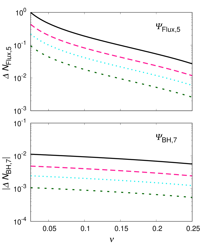
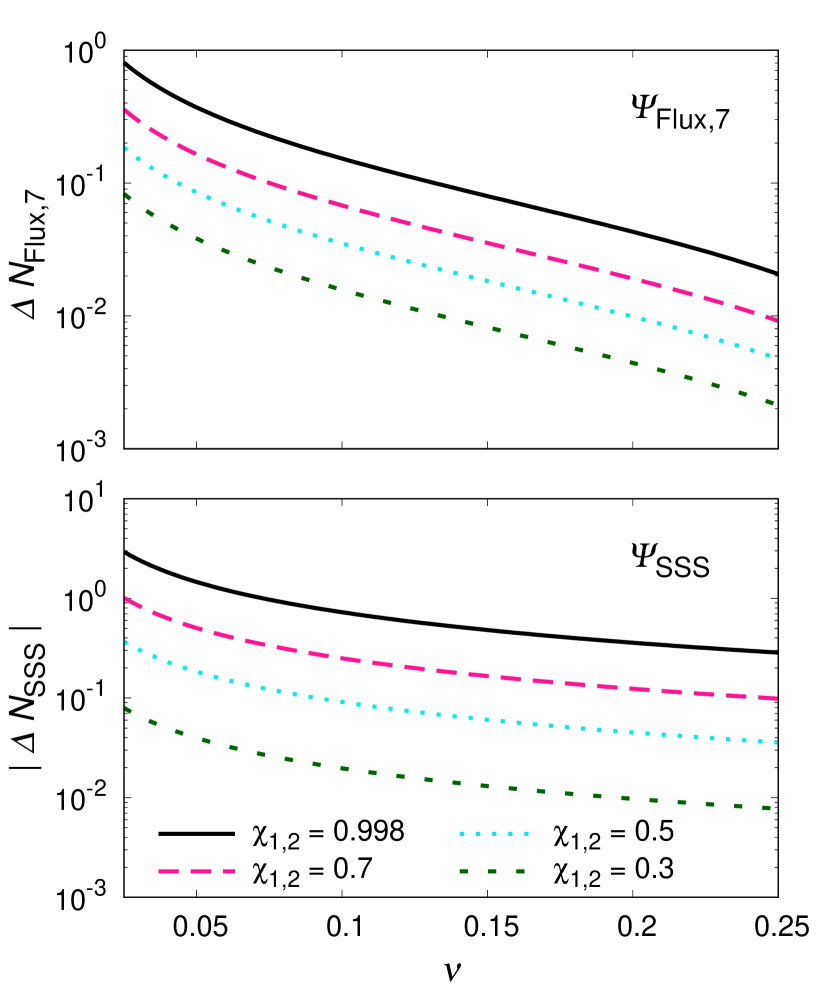
Figure 1: The relative number of GW cycles $\Delta N$ accumulated in ground based detectors, LIGO/VIRGO/KAGRA frequency band $mf\in[0.0035,\,0.018]$ as a function of the initial symmetric mass ratio $\nu$ for different values of the initial aligned spins $\chi_{1}=\chi_{2}$, for the contribution of the LO horizon-flux term $\Psi^{\mathrm{F2}}_{\mathrm{Flux},5}$ (Top left), the NLO horizon-flux term $\Psi^{\mathrm{F2}}_{\mathrm{Flux},7}$ (Top right), the LO term due to the secular change in BH intrinsic parameters $\Psi^{\mathrm{F2}}_{\mathrm{BH},7}$ (Bottom left) and (for comparison) the LO cubic-in-spin term without the BH absorption $\Psi^{\mathrm{F2}}_{\mathrm{SSS}}$ (Bottom right). A nearly extremely spinning BBH with $\chi_{1,2}=0.998$ is in the Novikov-Thorne limit for BHs spun up by accretion [86]. For $\Delta N_{\mathrm{BH},7}$ and $\Delta N_{\mathrm{SSS}}$, their absolute values $|\Delta N_{\mathrm{BH},7}|$ and $|\Delta N_{\mathrm{SSS}}|$ are plotted because they become negative in this parameter region.

Figure 1 shows the contributions of $\Psi^{\mathrm{F2}}_{\mathrm{Flux},5}$, $\Psi^{\mathrm{F2}}_{\mathrm{Flux},7}$ and $\Psi^{\mathrm{F2}}_{\mathrm{BH},7}$ (including their prefactors in (1.7)) to $\Delta N_{\mathrm{Flux},5}$, $\Delta N_{\mathrm{Flux},7}$ and $\Delta N_{\mathrm{BH},7}$, respectively, as a function of the initial value of the mass ratio $\nu$ with different initial values of the aligned spins $\chi_{1}=\chi_{2}$ accumulated within the GW frequency $mf\in[0.0035,\,0.018]$ in terms of the initial total mass $m$. The choice of our frequency band comes from the fact that this agrees with the inspiral portion of the “PhenomD” model [44] and thus it is the most relevant band for plausible BBH parameters measured by ground-based GW detector such as Advanced LIGO, Advanced Virgo and KAGRA. For comparison, we also show the same results for the cubic-in-spin pieces $(3v^{2}\Psi^{\mathrm{F2}}_{\mathrm{SSS}})/(128\nu)$ in the point-particle phase $\Psi^{\mathrm{F2}}_{\infty}(v)$, which generates $\Delta N_{\mathrm{SSS}}$ at $3.5$PN order [see (4.127)]. In this case, we find that individual contributions $\Delta N_{\mathrm{Flux},5},\Delta N_{\mathrm{Flux},7}$ and $\Delta N_{\mathrm{BH},7}$ are all negligible. They are always smaller than $|\Delta N_{\mathrm{SSS}}|$ and, in particular, the value of $\Delta N_{\mathrm{BH},7}$ is highly suppressed due to the prefactor $\nu$ for $\Psi^{\mathrm{F2}}_{\mathrm{BH},7}$ in (1.7); we have $\Delta N_{\mathrm{BH},7}\sim\nu^{0}$ while others scale as $\Delta N_{\mathrm{Flux},5}\sim\Delta N_{\mathrm{Flux},7}\sim\Delta N_{\mathrm{SSS}}\sim\nu^{-1}$. We also note that the magnitude of $\Delta N_{\mathrm{Flux},5},\Delta N_{\mathrm{Flux},7},\Delta N_{\mathrm{BH},7}$ and $\Delta N_{\mathrm{SSS}}$ become smaller for BBHs with the same magnitude of spins anti-aligned with the orbital angular momentum. These results are consistent with the previous study by Alvi [57], where for BBHs with the total mass $m$ ranging from $5.0M_{\odot}$ to $50.0M_{\odot}$ and aligned spins $\chi_{1,2}=0.998$, only negligible contribution of $\Delta N_{\mathrm{Flux},5}$ is observed.

However, we find that the sum of $\Delta N_{\mathrm{Flux},5}$ and $\Delta N_{\mathrm{Flux},7}$ are marginally non-negligible for BBHs with high-mass ratio $\nu\lesssim 0.05$ and high spins $\chi_{1,2}\gtrsim 0.90$. In figure 1, we see that NLO ($3.5$PN) horizon-flux contribution $\Delta N_{\mathrm{Flux},7}$ can be as much as LO ($2.5$PN) horizon-flux contribution $\Delta N_{\mathrm{Flux},5}$. The origin of these comparable contributions can be easily understood from the fact that for the given $\nu$ and $\chi_{1,2}$ the NLO phase coefficient $\Psi^{\mathrm{F2}}_{\mathrm{Flux},7}$ in (1.7) [or (4.140)] is $O(10)$ larger than the LO phase coefficient $\Psi^{\mathrm{F2}}_{\mathrm{Flux},5}$. Because of this, the corresponding NLO horizon-flux term in the integrand (1.10) also becomes larger than the LO horizon-flux term when $mf\gtrsim 0.0110$ in our case. In fact, the sum of $\Delta N_{\mathrm{Flux},5}$ and $\Delta N_{\mathrm{Flux},7}$ are almost the same as the cubic-in-spin contribution $\Delta N_{\mathrm{SSS}}$ and they could compensate each other; recall that $\Delta N_{\mathrm{SSS}}$ is negative while $\Delta N_{\mathrm{Flux},5}$ and $\Delta N_{\mathrm{Flux},7}$ are positive. Therefore, by contrast to the prior belief [57], the horizon-flux contributions to the number of GW cycles $N$ could be marginally non-negligible when we account for both the LO and NLO terms.

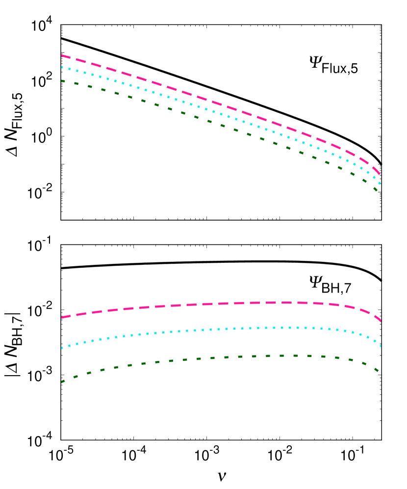
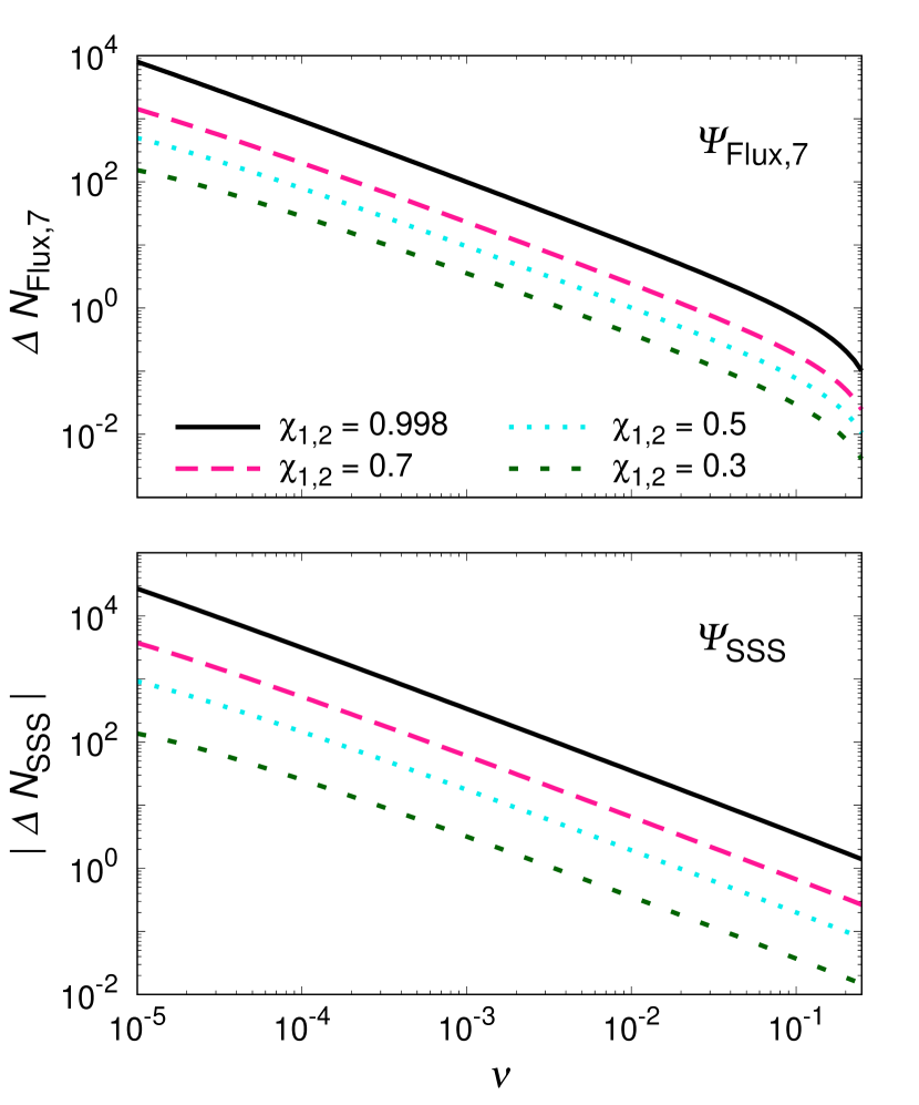
Figure 2: The relative number of GW cycles $\Delta N$ accumulated in a space based detector, LISA frequency band $mf\in[2.0\times 10^{-4}\,\nu^{-3/8},\,mf_{\mathrm{ISCO}}]$ as a function of the initial symmetric mass ratio $\nu$ for different values of the initial aligned spins $\chi_{1}=\chi_{2}$. For $\chi_{1,2}=0.998$, the upper cutoff of the frequency is $mf_{\mathrm{pole}}\sim 0.109$, which is smaller than the ISCO frequency $mf_{\mathrm{ISCO}}\sim 0.134$, to validate TaylorF2 model. Labels are the same as for figure 1, and we plot the absolute value of $\Delta N_{\mathrm{BH},7}$ and $\Delta N_{\mathrm{SSS}}$ as they become negative in the given parameter region.

Figure 2 is similar to figure 1 except that the frequency band is now chosen as $mf\in[2.0\times 10^{-4}\nu^{-3/8},\,mf_{\mathrm{ISCO}}]$, where $f_{\mathrm{ISCO}}$ is twice the frequency of the innermost stable circular orbit (ISCO) for Kerr geometry with mass $m$ and aligned equal-spin $\chi_{1,2}$ [87], namely,

$$\pi mf_{\mathrm{ISCO}}\equiv\{(3+Z_{2}-[(3-Z_{1})(3+Z_{1}+2Z_{2})]^{1/2})^{3/2}+\chi_{1,2}\}^{-1}$$ (1.11)

with $Z_{1}\equiv 1+(1-\chi_{1,2}^{2})^{1/3}[(1+\chi_{1,2})^{1/3}+(1-\chi_{1,2})^{1/3}]$ and $Z_{2}\equiv(3\chi_{1,2}^{2}+Z_{1}^{2})^{1/2}$. Roughly speaking, the choice of this frequency band is motivated by the one year observation of BBHs with the initial total mass $m\sim O(10^{6})M_{\odot}$ before reaching ISCO [88], and this covers plausible BBH parameters for LISA. In this case, the ech horizon-flux contribution $\Delta N_{\mathrm{Flux},5}$ and $\Delta N_{\mathrm{Flux},7}$ become non-negligible for BBHs with high-mass ratio $\nu\lesssim 0.01$ and moderate aligned-spins $\chi_{1,2}\gtrsim 0.50$. They rapidly grow as $\Delta N_{\mathrm{Flux},5}\sim\nu^{-1}\ln(\nu)$ and $\Delta N_{\mathrm{Flux},7}\sim\Delta N_{\mathrm{SSS}}\sim\nu^{-5/4}$ as $\nu$ decreases, and their values become as large as $O(10^{3})\sim O(10^{4})$ when $\nu\sim 10^{-5}$, depending on the values of $\chi_{1,2}$. While our results for high-mass-ratio inspirals $(\nu\lesssim 10^{-3})$ are only indicative because the PN approximation is not so accurate for these BBHs [89, 90, 91, 92], these results are basically consistent with previous results made by many authors, which showed that for quasicircular, extreme mass-ratio BBH inspirals with $\nu\sim 10^{-6}$ and nearly extremal spins the horizon-flux effects significantly increases the duration of inspiral phase [65, 68, 69, 70].

Meanwhile, figure 2 shows that $\Delta N_{\mathrm{BH},7}$ is negligible even for the LISA-type detector. One would question this result because the scaling $\Delta N_{\mathrm{BH},7}\sim\nu^{-1/4}$ is expected given the prefactor $\nu$ for $\Psi^{\mathrm{F2}}_{\mathrm{BH},7}$ in (1.7), and it could be pronounced when $\nu$ is sufficiently small. However, the explicit calculation shows that its coefficient that depends on the spins is at most $O(10^{-3})$ even when $\chi_{1,2}=0.998$. Given the range of mass ratio that we consider here, the term $\Delta N_{\mathrm{BH},7}\sim\nu^{-1/4}$ therefore does not dominate compared to other $\nu$-dependent terms in $\Delta N_{\mathrm{BH},7}$, which have the positive powers in $\nu$.

1.4 Results 2: the mismatch for Advanced LIGO and LISA

While the GW detectors are sensitive to the evolution of the GW phase of BBH inspirals, the relative number of GW cycles $\Delta N_{\mathrm{Flux},5}$, $\Delta N_{\mathrm{Flux},7}$ and $\Delta N_{\mathrm{BH},7}$ accumulated in a detector’s frequency-band is not a robust estimator for the amount of information contained in each phase correction $\Psi^{\mathrm{F2}}_{\mathrm{Flux},5},\Psi^{\mathrm{F2}}_{\mathrm{Flux},7}$ and $\Psi^{\mathrm{F2}}_{\mathrm{BH},7}$. For the measurement of BBHs by Advanced LIGO and LISA, such information becomes manifest only when aided by the matched filtering [18].

In section 5, we compute an optimized cross-correlation (usually called match [93, 94]) between the two TaylorF2 waveforms with and without each phase correction $\Psi^{\mathrm{F2}}_{\mathrm{Flux},5},\Psi^{\mathrm{F2}}_{\mathrm{Flux},7}$ and $\Psi^{\mathrm{F2}}_{\mathrm{BH},7}$ due to BH absorption as a measure of template imperfection; the definition of the match is detailed below in section 5.1. The match is weighted by the detector noise spectrum that we hope to observe the GW signal with, and can quantify the faithfulness [95] of our PN template in observing GW signals of BBHs by Advanced LIGO and LISA. A match of unity means that the template is a very precise representation of the target GW signal. A value less than unity means that the template reproduces the signal only imperfectly and hence it is unfaithful. We below consider that the mismatch ($\equiv$ 1 - match) due to template imperfection is significant if it is larger than $3\%$ [95].

We compute the match by taking the target GW signal to be the TaylorF2 waveforms in (1.6) with the complete $3.5$PN phase $\Psi^{\mathrm{F2}}_{3.5{\mathrm{PN}}}$ in (1.7), and by taking five different templates to be the same TaylorF2 waveforms as the target signal except each template neglects one of the following phase contributions: (1) the LO horizon-flux term $\Psi^{\mathrm{F2}}_{\mathrm{Flux},5}$; (2) the NLO horizon-flux term $\Psi^{\mathrm{F2}}_{\mathrm{Flux},7}$; (3) the LO term due to the secular change in BH mass and spins $\Psi^{\mathrm{F2}}_{\mathrm{BH},7}$; (4) all phase terms due to BH absorption $\Psi^{\mathrm{F2}}_{\mathrm{H,all}}=\{\Psi^{\mathrm{F2}}_{\mathrm{Flux},5},\,\Psi^{\mathrm{F2}}_{\mathrm{Flux},7},\,\Psi^{\mathrm{F2}}_{\mathrm{BH},7}\}$; (5) (for comparison) the LO cubic-in-spin term $\Psi^{\mathrm{F2}}_{\mathrm{SSS}}$ in the non-absorption, point-particle phase term $\Psi^{\mathrm{F2}}_{\infty}$ [recall (1.7)]. The match for Advanced LIGO accounts for the noise curve of its “zero-detuning, high-power” configuration [96] [see (5.5)], which is the design goal of Advanced LIGO, and we consider the frequencies in the interval $mf\in[0.0035,\,0.018]$, using the same setup in figure 1. At the same time, the match for LISA takes into account its latest noise curve [97], which includes the improvement successfully demonstrated by LISA Pathfinder [98] [see (5.7)], and we chose the frequency range $mf\in[2.0\times 10^{-4}\,\nu^{-3/8},\,mf_{\mathrm{ISCO}}]$ with twice the frequency of the ISCO for Kerr geometry $f_{\mathrm{ISCO}}$ [recall (1.11)], in order to echo to the setup in figure 2. The rationale for our choice of the frequency range is that we are interested in analyzing the (dis)agreement of TaylorF2 with and without the correction due to BH absorption, and our interval can provide a baseline for fair comparison between such two different TaylorF2; recall that the different choice for the frequency range affects each template in the same way. A full discussion about mismatch calculation is presented in section 5.2.

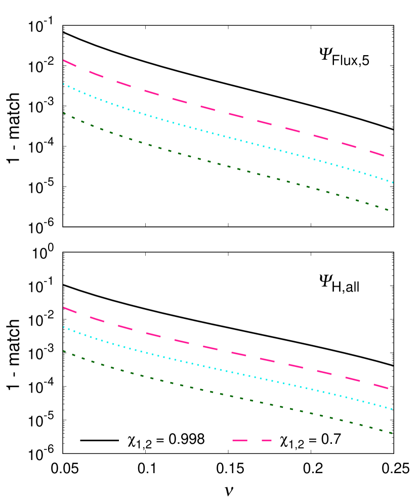
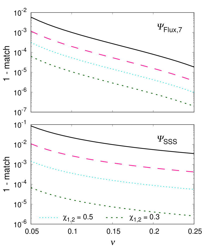
Figure 3: The mismatch ($\equiv 1-{\mathrm{match}}$) between the two TaylorF2 templates with and without each phase correction due to BH absorption accumulated in the Advanced LIGO frequency band $mf\in[0.0035,\,0.018]$, where the initial total mass chosen to be $m=60.0M_{\odot}$. The results are plotted as a function of the symmetric mass ratio $\nu$ for different values of the initial aligned-spins $\chi_{1}=\chi_{2}$, and they are grouped into four panels according to what is neglected in the TaylorF2 phase in (1.7); Top left: the neglect of the LO horizon-flux term $\Psi^{\mathrm{F2}}_{\mathrm{Flux},5}$. Top right: the neglect of the NLO horizon-flux term $\Psi^{\mathrm{F2}}_{\mathrm{Flux},7}$. Bottom left: the neglect of all phase terms due to BH absorption $\Psi^{\mathrm{F2}}_{\mathrm{H,all}}$, including all horizon-flux terms $\Psi^{\mathrm{F2}}_{\mathrm{Flux},5}$ and $\Psi^{\mathrm{F2}}_{\mathrm{Flux},7}$ as well as the LO term due to the secular change in BH intrinsic parameters $\Psi^{\mathrm{F2}}_{\mathrm{BH},7}$. Bottom right: (for comparison) the neglect of the LO cubic-in-spin term $\Psi^{\mathrm{F2}}_{\mathrm{SSS}}$ in the non-absorption, point-particle phase term $\Psi^{\mathrm{F2}}_{\infty}$.

For BBHs observable by Advanced LIGO, we summarize the mismatch for each imperfect template with our complete BH-absorption TaylorF2 in figure 3, assuming that the initial total mass of the BBH is $m=60.0M_{\odot}$ (this corresponds to $f\in[11.8,\,60.9]$ Hz) for different values of initial aligned-spins. Because the mismatch due to the neglect of $\Psi^{\mathrm{F2}}_{\mathrm{BH},7}$ is always below the $10^{-7}$ mark even with nearly extremal aligned-spins $\chi_{1,2}=0.998$, the corresponding mismatch is not displayed here.

Overall, the mismatch in figure 3 follows the similar trend for the relative contribution to GW cycles $\Delta N$ in figure 1 and supports the broader conclusion that we can draw from it; the effects BH absorption on GWs are significant for high-mass-ratio, high-aligned-spin BBHs. More specifically, not including the phase term $\Psi^{\mathrm{F2}}_{\mathrm{H,all}}$ introduces the significant mismatch when the BBH is in high-mass ratio regime $\nu\lesssim 0.083$ with nearly extremal aligned-spins $\chi_{1,2}\sim 0.098$ as well as at very high-mass ratio region $\nu\lesssim 0.05$ with large aligned-spins $\chi_{1,2}\gtrsim 0.70$. Looking at top two panels, we particularly see that the inclusion of $\Psi^{\mathrm{F2}}_{\mathrm{Flux},5}$ is crucial as this dominates the mismatch due to the neglect of $\Psi^{\mathrm{F2}}_{\mathrm{H,all}}$; by contrast to $\Delta N_{\mathrm{Flux},7}$ in figure 1 the mismatch due to neglecting $\Psi^{\mathrm{F2}}_{\mathrm{Flux},7}$ never becomes significant for BBHs considered here. In the bottom two panels, we also see that the mismatch due to neglecting $\Psi^{\mathrm{F2}}_{\mathrm{SSS}}$ is as significant as that of $\Psi^{\mathrm{F2}}_{\mathrm{H,all}}$; recall that $\Psi^{\mathrm{F2}}_{\mathrm{H,all}}$ consists of both linear-in-spin and cubic-in-spin terms [see (4.140)]. This suggests that one would also need to include $\Psi^{\mathrm{F2}}_{\mathrm{SSS}}$ if we wish to fully exploit information about BH absorption in $\Psi^{\mathrm{F2}}_{\mathrm{H,all}}$ by measuring BBHs by Advanced LIGO.

We emphasize that the mismatch in figure 3 is only indicative; the resulting mismatch depends on the upper and lower cutoff frequencies that we consider here. Their interpretation in the context of actual GW search is thus delicate. For instance, if we instead take the frequency interval $mf\in[0.0035,\,mf_{\mathrm{ISCO/pole}}]$, the mismatch plotted in figure 3 is increased by a factor of $O(10)$. In this case, the mismatch due to neglecting $\Psi^{\mathrm{F2}}_{\mathrm{H,all}}$ can be above the $3\%$ mark even for the high-mass-ratio BBH $(\nu\lesssim 0.10)$ with moderate aligned-spins ($\chi_{1,2}\gtrsim 0.50)$ as well as the almost equal-mass ratio BBH $(\nu\lesssim 0.20)$ with near extremal aligned-spins $(\chi_{1,2}\sim 0.998)$. Another example is the frequency interval $mf\in[10.0m,\,845.0]$ considered by Alvi [57]. For BBHs with the initial total mass $m=\{5.0,20.0,50.0\}M_{\odot}$ and the initial aligned-spins $\chi_{1,2}=0.998$, Alvi showed for such BBHs with symmetric mass ratio $\nu\gtrsim 0.16$ (corresponding to $m_{2}/m_{1}\leq 4$) that $\Delta N_{\mathrm{Flux},5}$ accumulated in his frequency range is far less than one radian; see Table IV of [57]. Focusing on his configurations $m=20(50)M_{\odot}$ with the mass ratio $\nu=\{0.25,0.22,0.16\}$ (corresponding to his choice $m_{2}/m_{1}=\{1,2,4\}$), however, we find that the neglect of $\Psi^{\mathrm{F2}}_{\mathrm{Flux},5}$ accumulated in the same frequency range produces the mismatch $0.74\%(0.37\%),\,1.7\%(0.87\%)$ and $7.1\%(3.8\%)$, respectively. While these values have no direct implication to an actual GW search for BBHs, we feel that more investigation would be needed to assess if the corrections $\Psi^{\mathrm{F2}}_{\mathrm{Flux},5}$ as well as $\Psi^{\mathrm{F2}}_{\mathrm{H,all}}$ in a realistic template are truly too small to be observed in current ground-based detectors, including Advanced LIGO/Virgo and KAGRA.

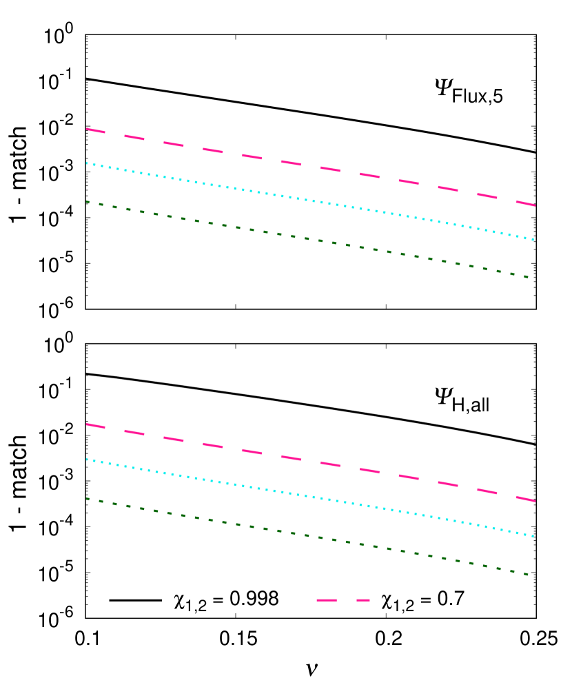
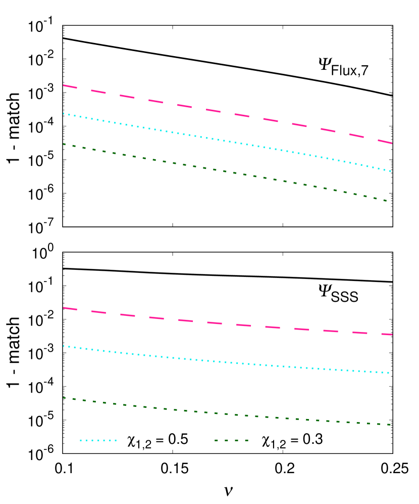
Figure 4: The mismatch ($\equiv 1-{\mathrm{match}}$) between the two TaylorF2 templates with and without each phase correction due to BH absorption accumulated in a space based detector, LISA frequency band $mf\in[2.0\times 10^{-4}\,\nu^{-3/8},\,mf_{\mathrm{ISCO}}]$, where the initial total mass is chosen to be $m=10^{6}M_{\odot}$. For $\chi_{1,2}=0.998$, the upper cutoff of the frequency is $mf_{\mathrm{pole}}\sim 0.109$. The label and grouping of the panels are the same as for figure. 3.

Figure 4 is similar to figure 3 except that it summarizes the mismatch of each imperfect template for supermassive BBHs observable by LISA, assuming that the initial total mass of the BBHs is $m=10^{6}M_{\odot}$ (corresponding, e.g., $f\lesssim 0.022$Hz for nearly extremal aligned-spins ${\chi}_{1,2}=0.998$). Because our TaylorF2 is not expected to be reliable for very high mass-ratio configuration ($\nu\lesssim O(10^{-2})$), we only consider supermassive BBHs with low mass-ratio in the range $\nu\in[0.10,\,0.25]$ . As was the case for BBHs observable by Advanced LIGO, figure 4 supports the broader conclusion that we can draw from the figure 2, which showed the relative contribution to GW cycles $\Delta N$; the mismatch due to the neglect $\Psi^{\mathrm{F2}}_{\mathrm{H,all}}$ is significant when supermassive BBHs is in almost equal-mass regime $\nu\lesssim 0.19$ with nearly extremal aligned-spins ${\chi}_{1,2}\gtrsim 0.998$ as well as in the moderate mass-ratio regime $\nu\lesssim 0.10$ with large aligned-spins $\chi_{1,2}\gtrsim 0.70$. For the case of LISA, we also see that the mismatch from neglecting $\Psi^{\mathrm{F2}}_{\mathrm{Flux},7}$ can become significant if the BBH is at large mass ratio $\nu\sim 0.1$ with nearly extremal aligned-spins ${\chi}_{1,2}\gtrsim 0.998$. This suggests that the NLO contribution $\Psi^{\mathrm{F2}}_{\mathrm{Flux},7}$ is likely to be as important as LO contribution $\Psi^{\mathrm{F2}}_{\mathrm{Flux},5}$ for measuring high-mass-ratio, high-aligned-spin supermassive BBHs. However, the mismatch due to the neglect of $\Psi^{\mathrm{F2}}_{\mathrm{BH},7}$ never becomes significant for all supermasiive BBHs that we consider here. The resulting mismatch is always below $10^{-5}$ mark, and we therefore do not plot it in figure 4.

It is interesting to observe that for supermassive BBHs in the large-spin regime ($\chi_{1,2}\gtrsim 0.70$), the mismatch from neglecting $\Psi^{\mathrm{F2}}_{\mathrm{SSS}}$ depends on the mass ratio only weakly. It becomes therefore significant over the full range of mass ratios. In addition, $\Psi^{\mathrm{F2}}_{\mathrm{SSS}}$ produces the larger mismatch than that from $\Psi^{\mathrm{F2}}_{\mathrm{H,all}}$ unless supermasiive BBHs have relatively small aligned-spins $\chi_{1,2}\lesssim 0.50$. This prompts us to suggest that the contribution $\Psi^{\mathrm{F2}}_{\mathrm{SSS}}$ to the PN template should not be neglected for supermassive BBHs to measure the BH-absorption effects by LISA.

Before concluding our paper, once more, we should point out that the mismatch presented in figure 4 is only indicative as its value is quite sensitive to our choice of the frequency range. If the upper cutoff frequency is instead chosen as twice of the frequency of the ISCO of the Schwarzschild space time $mf_{\mathrm{ISCO,Sch}}(\sim 0.022)\ll mf_{\mathrm{pole}}(\sim 0.109)$ [recall (1.11)], all mismatch plotted in figure. 4 is decreased by a factor of $O(10)$. We find, nevertheless, that our results give a useful idea about the impact of BH absorption in the context of LISA, and we expect this helps future modeling efforts for GWs from suppermassive BBHs.

In summary, we found the following four main results:

1. For the case of BBHs observable by Advanced LIGO, not including the LO horizon-flux phase term $\Psi^{\mathrm{F2}}_{\mathrm{Flux},5}$ will typically cause a significant phasing error in PN templates if BBHs are in high-mass ratio $(\nu\lesssim 0.10)$ and high aligned-spins $({\chi}_{1,2}\gtrsim 0.70)$ regime;

2. For the case of supermassive BBHs observable by LISA, the inclusion of both $\Psi^{\mathrm{F2}}_{\mathrm{Flux},5}$ and $\Psi^{\mathrm{F2}}_{\mathrm{Flux},7}$ in PN templates will be mandatory. Almost equal-mass supermassive BBHs $(\nu\lesssim 0.20)$ with nearly extremal aligned-spins $({\chi}_{1,2}\sim 0.998)$ can produce significant phasing errors if they are neglected, and they become more evident for the lower-spin BBHs with decreasing mass-ratio;

3. The phasing error due to the LO secular change in BH masses and spins $\Psi^{\mathrm{F2}}_{\mathrm{BH},7}$ is truly negligible for all BBHs measurable by Advanced LIGO and LISA;

4. The $3.5$PN cubic-in-spin phase term $\Psi^{\mathrm{F2}}_{\mathrm{SSS}}$ in the non-absorption, point-particle phase term $\Psi^{\mathrm{F2}}_{\infty}$ [recall (1.7)] causes the significant phasing error as much as $\Psi^{\mathrm{F2}}_{\mathrm{H,all}}$, thus should not be neglected when one includes the correction due to BH absorption to PN templates.

A note on the limitation of this work— Our work is intended as a proof-of-principle, hence there are various limitations, which are summarized as follows.

First, our templates did not account for the precession effects in BBHs; despite its importance, for example, in the detection of BBHs by Advanced LIGO [99, 100], the (PN) computation of the horizon flux for the spin-precessing BBHs is beyond the current state of the art, even in the test spinning-particle limit. Second, we considered only the dominant $(2,2)$ spin-weighted-spherical-harmonic mode of GW waveforms, and neglected the contribution from their higher harmonics. For the case of BBH with high-mass-ratio and high-spins, these modes can be significant during the last stages of inspiral [80] and the corresponding systematic errors to the templates due to neglecting such higher modes become larger [101, 102]. While the main goal of this paper motivates us to limit the scope to the dominant $(2,2)$ mode, our work could be improved by the corrections from these higher modes, for instance, making use of the method recently proposed in [103]. Third, although there have been highly accurate predictions for inspiral, merger and ringdown gravitational waveforms for BBHs, we did not use the effective-one-body waveforms [37] or the phenomenological (so-called PhenomD) waveforms [44] as our reference GW signals. As seen in figures 3 and 4, the corrections to the template due to BH absorption become most significant in high-mass-ratio regime with high aligned-spins, but very few NR simulation is currently available there. These models therefore are not well calibrated for such “extreme” BBHs. Given the spirit of this work, we rather focus on only the (early) inspiral phase, sticking to use the simple TaylarF2 model in the GW frequency range $mf\leq 0.018$ for Advanced LIGO and $f\leq f_{\mathrm{ISCO}}$ for LISA. In these cases, the resulting matches would be difficult to interpret as they have no immediate application in actual GW searches for BBHs, but they provide a conceptually clean setup to study the impact of BH absorption on the template.

Despite such limitations, we feel that our findings in this paper would motivate further explorations of GW data-analysis tasks for spinning, non-precessing BBHs. The impact of BH absorption for parameter-estimate predictions for LIGO-type and LISA-type detectors could be investigated in future work. The issue of the corresponding systematic biases in (PN) template families due to the effect of BH absorption would be also a relevant extension of our work; systematic errors in GW observations was already discussed in the context of neutron-star binaries [104, 105, 106] as well as BBHs [27, 107, 108].

In the remainder of the paper, we detail the results presented above. In section 2, we summarize the PN expressions for the center-of-mass binding energy, the GW energy flux to infinity and the horizon energy fluxes. Then, the secular change in BH masses and spins is calculated. In section 3, we present the corrected binding energy and GW energy flux as well as the generalized balance equation that include the appropriate effects of the secular change in the BH mass and spin during the inspiral phase. The PN template families from the generalized balance equation are given in section 4. Finally in section 5 we calculate the match between frequency-domain PN templates with and without the effect of BH absorption. The mismatch for other BBH configurations that were not covered in this section are displayed in section 5.3.

2 The PN approximants

For the convenience of the reader, we in this section recapitulate the explicit $3.5$PN expressions for the center-of-mass binding energy $E$, the GW energy flux carried out to infinity ${F}_{\infty}$ and the horizon energy (and angular momentum) fluxes ${\cal F}_{\mathrm{H}}^{i}\,(i=1,\,2)$ for the pinning, non-precessing quasicircular BBH with constant masses $m_{i}$ and constant-in-magnitude spin vectors ${\bf S}_{i}$, beyond their LO Newtonian terms. We shall import many relevant results from the review [20] and references [62, 67, 109] as well as literatures cited in these references. We then compute the LO PN expressions for the secular change in the BH mass and spin during the inspiral phase, which are at $3.5$PN and $2$PN order, respectively.

Following the notation used in [20], we define the projected value of the spin vectors ${\bf{S}}_{i}$ along the unit normal ${\bm{\ell}}$ to the orbital plane by ${S}_{i}\equiv{\bf{S}}_{i}\cdot{\bm{\ell}}$, and introduce two combinations of them:

$$S_{\ell}\equiv{S_{1}}+{S_{2}}\,,\quad\Sigma_{\ell}\equiv\frac{{S_{2}}}{X_{2}}-\frac{{S_{1}}}{X_{1}}\,,$$ (2.1)

where $X_{i}\equiv m_{i}/m$. We here also introduce the dimensionless spin parameter $\chi_{i}$ by

$${\chi}_{i}\equiv\frac{S_{i}}{m_{i}^{2}}\,.$$ (2.2)

In our notation, the spin parameter takes $-1<{\chi}_{i}<1$; its positive (negative) value corresponds to the aligned (anti-aligned) configuration with respect to the orbital angular momentum of the binary. Assuming $m_{1}<m_{2}$, (2.1) and (2.2) are related by

$$S_{\ell} =\frac{m^{2}}{4}(1+\Delta)^{2}\chi_{1}+\frac{m^{2}}{4}(1-\Delta)^{2}\chi_{2}\,,$$ (2.3)

$$\Sigma_{\ell} =-\frac{m^{2}}{2}(1+\Delta)\chi_{1}+\frac{m^{2}}{2}(1-\Delta)\chi_{2}\,,$$ (2.4)

which can be inverted to give

$$\chi_{1}=\frac{2\{(1+\Delta)S_{\ell}-2\nu\Sigma_{\ell}\}}{m^{2}(1+\Delta)^{2}}\,,\quad\chi_{2}=\frac{2\{(1-\Delta)S_{\ell}+2\nu\Sigma_{\ell}\}}{m^{2}(1-\Delta)^{2}}\,,$$ (2.5)

where

$$\Delta\equiv-\sqrt{1-4\nu}\,,\quad\nu\equiv\frac{m_{1}m_{2}}{m^{2}}=X_{1}X_{2}\,.$$ (2.6)

2.1 The binding energy and the energy flux emitted to the infinity

Schematically, the $3.5$PN binding energy is expressed as

$$E\equiv-\frac{m\nu}{2}v^{2}\left(E_{\mathrm{NS}}+\frac{v^{3}}{m^{2}}E_{\mathrm{SO}}+\frac{v^{4}}{m^{4}}E_{\mathrm{SS}}+\frac{v^{7}}{m^{6}}E_{\mathrm{SSS}}+O(v^{8})\right)\,,$$ (2.7)

where $E_{\mathrm{NS}},E_{\mathrm{SO}},E_{\mathrm{SS}}$ and $E_{\mathrm{SSS}}$ denote the non-spinning, spin-orbit (SO, linear-in-spin), spin-spin (SS, quadratic-in-spin), and spin-spin-spin (SSS, cubic-in-spin) contributions to $E$ and all depend on the parameters $m,\nu,S_{\ell}$ and $\Sigma_{\ell}$ as a function of $v$. Their explicit expressions are provided in (232) and (415) of [20] for $E_{\mathrm{NS}}$ and $E_{\mathrm{SO}}$ respectively, in (3.33) of [109] for $E_{\mathrm{SS}}$ and in (6.17) of [67] for $E_{\mathrm{SSS}}$. The expressions for $E_{\mathrm{SS}}$ and $E_{\mathrm{SSS}}$ include constants $\kappa_{\pm}$ and $\lambda_{\pm}$ that characterize the deformation of a small object in a binary due to its own spin angular-momentum, and they take $\kappa_{+}=\lambda_{+}=2$ and $\kappa_{-}=\lambda_{-}=0$ for a BBH [67, 109]. The expressions are then given by

$$E_{\mathrm{NS}} =1+\left(-\frac{3}{4}-\frac{1}{12}{\nu}\right)v^{2}+\left(-\frac{27}{8}+\frac{19}{8}\nu-\frac{1}{24}\nu^{2}\right){v}^{4}$$ (2.8)

$$\quad+\left\{-\frac{675}{64}+\left(\frac{34445}{576}-\frac{205\,{\pi}^{2}}{96}\right)\nu-\frac{155}{96}\nu^{2}-\frac{35}{5184}\nu^{3}\right\}{v}^{6}\,,$$ (2.9)

$$E_{\mathrm{SO}} =\left(\frac{14}{3}\,S_{\ell}+2\Delta\Sigma_{\ell}\right)+\left\{\left(11-\frac{61}{9}\nu\right)S_{\ell}+\left(3-\frac{10}{3}\nu\right)\Delta\,\Sigma_{\ell}\right\}v^{2}$$ (2.10)

$$\quad+\left\{\left({\frac{135}{4}}-\frac{367}{4}\nu+\frac{29}{12}\nu^{2}\right)S_{\ell}+\left(\frac{27}{4}-39\,{\nu}+\frac{5}{4}\,{\nu}^{2}\right)\Delta\,\Sigma_{\ell}\right\}{v}^{4}\,,$$ (2.11)

$$E_{\mathrm{SS}} =-4S^{2}_{\ell}-4\Delta\Sigma_{\ell}S_{\ell}-(1-4\nu)\Sigma_{\ell}^{2}$$ (2.12)

$$\quad+\left\{\left(-\frac{25}{9}+\frac{10}{3}\,\nu\right)S_{\ell}^{2}+\left(\frac{10}{3}+\frac{10}{3}\,{\nu}\right)\Delta\Sigma_{\ell}S_{\ell}+\left(\frac{5}{2}-\frac{15}{2}\nu-\frac{10}{3}\nu^{2}\right)\Sigma_{\ell}^{2}\right\}v^{2}\,,$$ (2.13)

$$E_{\mathrm{SSS}} =-8S_{\ell}^{3}-16\Delta\Sigma_{\ell}{S}_{\ell}^{2}-10(1-4\nu)\Sigma_{\ell}^{2}S_{\ell}-2(1-4\nu)\Delta\Sigma_{\ell}^{3}\,.$$ (2.14)

We note that $E$ is complete up to the relative 3.5PN order.

Similarly, the $3.5$PN energy flux associated with gravitational radiation carried out to infinity is written as

$${F}_{\infty}\equiv\frac{32}{5}\nu^{2}v^{10}\left({F}_{\mathrm{NS}}+\frac{v^{3}}{m^{2}}{F}_{\mathrm{SO}}+\frac{v^{4}}{m^{4}}{F}_{\mathrm{SS}}+\frac{v^{7}}{m^{6}}{F}_{\mathrm{SSS}}+O(v^{8})\right)\,,$$ (2.15)

where ${F}_{\mathrm{NS}},{F}_{\mathrm{SO}},{F}_{\mathrm{SS}}$ and ${F}_{\mathrm{SSS}}$ denote the non-spinning, SO, SS, and SSS parts of ${F}_{\infty}$ and all depend on the parameters $m,\nu,S_{\ell}$ and $\Sigma_{\ell}$ as a function of $v$. Their explicit expressions are provided in (314) and (414) of [20] for ${F}_{\mathrm{NS}}$ and ${F}_{\mathrm{SO}}$ respectively, in (4.14) of [109] for ${F}_{\mathrm{SS}}$ and in (6.19) of [67] for ${F}_{\mathrm{SSS}}$. Once again setting $\kappa_{\pm}$ and $\lambda_{\pm}$ in ${F}_{\mathrm{SS}}$ and ${F}_{\mathrm{SSS}}$ as $\kappa_{+}=\lambda_{+}=2$ and $\kappa_{-}=\lambda_{-}=0$, their expressions for a BBH read

$${F}_{\mathrm{NS}} =1+\left(-\frac{1247}{336}-\frac{35}{12}\nu\right)v^{2}+4\,\pi\,{v}^{3}+\left(-\frac{44711}{9072}+\frac{9271}{504}\nu+\frac{65}{18}\nu^{2}\right){v}^{4}$$ (2.16)

$$\quad+\left(-\frac{8191}{672}-\frac{583}{24}\nu\right)\pi\,{v}^{5}+\left\{\frac{6643739519}{69854400}+\frac{16}{3}{\pi}^{2}-\frac{1712}{105}\,\gamma_{\rm E}-\frac{856}{105}\,\ln\left(16\,v^{2}\right)\right.$$ (2.17)

$$\quad+\left.\left(-\frac{134543}{7776}+\frac{41\,}{48}{\pi}^{2}\right)\nu-\frac{94403}{3024}\nu^{2}-\frac{775}{324}\nu^{3}\right\}{v}^{6}$$ (2.18)

$$\quad+\left(-\frac{16285}{504}+\frac{214745}{1728}\nu+\frac{193385}{3024}\nu^{2}\right)\pi\,{v}^{7}\,,$$ (2.19)

$${F}_{\mathrm{SO}} =-4\,S_{\ell}-\frac{5}{4}\Delta\,\Sigma_{\ell}+\left\{\left(-\frac{9}{2}+\frac{272}{9}\nu\right)S_{\ell}+\left(-\frac{13}{16}+\frac{43}{4}\nu\right)\Delta\,\Sigma_{\ell}\right\}v^{2}$$ (2.20)

$$\quad+\left(-16S_{\ell}-\frac{31}{6}\,\Delta\Sigma_{\ell}\right)\pi\,v^{3}$$ (2.21)

$$\quad+\left\{\left(\frac{476645}{6804}+\frac{6172}{189}\nu-\frac{2810}{27}\nu^{2}\right)S_{\ell}+\left(\frac{9535}{336}+\frac{1849}{126}\nu-\frac{1501}{36}\nu^{2}\right)\Delta\,\Sigma_{\ell}\right\}{v}^{4}\,,$$ (2.22)

$${F}_{\mathrm{SS}} =8{S}_{\ell}^{2}+8\Delta\Sigma_{\ell}S_{\ell}+\left(\frac{33}{16}-8\nu\right){\Sigma}^{2}_{\ell}-\left\{\left({\frac{3839}{252}}+43\nu\right){S}^{2}_{\ell}+\left(\frac{1375}{56}+43\nu\right)\Delta\Sigma_{\ell}S_{\ell}\right.$$ (2.23)

$$\quad\left.+\left(\frac{227}{28}-\frac{3481}{168}\nu-43{\nu}^{2}\right){\Sigma}^{2}_{\ell}\right\}v^{2}+O(v^{3})\,,$$ (2.24)

$${F}_{\mathrm{SSS}} =-\frac{16}{3}{S}_{\ell}^{3}+\frac{2}{3}\Delta\Sigma_{\ell}S_{\ell}^{2}+\left(\frac{9}{2}-\frac{56}{3}\nu\right){\Sigma}_{\ell}^{2}S_{\ell}+\left(\frac{35}{24}-6\nu\right)\Delta{\Sigma}_{\ell}^{3}\,,$$ (2.25)

where $\gamma_{\rm E}=0.577\dots$ are Euler constant. As we indicated in ${F}_{\mathrm{SS}}$ with the term of $O(v^{3})$, ${F}_{\infty}$ is incomplete because its $1.5$PN terms due to the SS tail contribution, which affects ${F}_{\infty}$ at the $3.5$PN order, are still unknown [109], except those in the test-particle limit $\nu\to 0$ [114, 115, 116]. These terms have yet to be computed in the future.

In addition, we note that ${F}_{\infty}$ has a pole at $v=v_{\mathrm{pole}}$ and become even negative when $v>v_{\mathrm{pole}}$. This unphysical behavior was first pointed out in the test-particle limit [117, 118], and the same issue happens for the finite-mass case. Fortunately, our examination suggests $v_{\mathrm{pole}}\gtrsim 0.70$ for a broad range of the BBH parameters, where the PN expansion will lose accuracy [89, 90, 91], and it should be taken over by the result from NR simulations. Moreover, if we compare the value of $v_{\mathrm{pole}}$ to the nominal value of the ISCO of the Kerr metric [recall (1.11)] with mass $m$ and (dimensionless) effective spin $\chi_{\mathrm{eff}}$ adopted in the phenomenological (“Phenom”) model [40, 41, 44]

$$\chi_{\mathrm{eff}}\equiv\frac{(1+\Delta)}{2}\chi_{1}+\frac{(1-\Delta)}{2}\chi_{2}\,,$$ (2.26)

we have $v_{\mathrm{ISCO}}\gtrsim 0.70$ only when $\chi_{\mathrm{eff}}\gtrsim 0.98$. These results assure that the pole in ${F}_{\infty}$ is not a serious obstacle in modeling BBHs during the inspiral phase except each individual BH has the nearly extremal spins, reaching the Novikov-Thorne limit $\chi_{1,2}=0.998$ for BHs spun up by accretion [86].

2.2 The horizon fluxes

Reference [62] provides the ready-to-use formulas of the horizon energy and angular-momentum fluxes for a BH in a quasicircular BBH, up to $1.5$PN order beyond the LO horizon fluxes, which are at $2.5$PN order beyond the quadrupolar fluxes. While their expressions at the relative $1.5$PN order do not recover the expressions in the test-particle limit $\nu\to 0$ [65, 68] , for the purpose of our analysis at the $3.5$PN accuracy level, we only need them up to the relative $1$PN order that do agree with the test-mass results. Importing the results in (42) and (43) of [62], the horizon energy and angular-momentum fluxes for the spinning, non-precessing, quasicircular BBH are defined by

$${\cal F}_{\mathrm{H}}^{i}\equiv\left\langle\frac{dm_{i}}{dt}\right\rangle=\Omega_{\mathrm{tidal}}(\Omega_{\mathrm{H}}-\Omega_{\mathrm{tidal}})\,C_{v,i}\,,$$ (2.27)

and

$$\left\langle\frac{d|S_{i}|}{dt}\right\rangle\equiv\Omega_{\mathrm{tidal}}^{-1}\left\langle\frac{dm_{i}}{dt}\right\rangle\,,$$ (2.28)

respectively; the angular-bracket operation in (2.27) and (2.28) indicates the long-term average [58]. Here, $t$ is the PN barycentric time, the angular velocity of the tidal field $\Omega_{\mathrm{tidal}}$ is

$$\Omega_{\mathrm{tidal}}=\epsilon_{i}\frac{v^{3}}{m}\left(1-\nu v^{2}+O(v^{3})\right)\,,$$ (2.29)

with $\epsilon_{i}=+1\,(-1)$ if the orbital and spin angular momentum of the unperturbed BH are aligned (anti-aligned), the angular velocity of the unperturbed Kerr BH is

$$\Omega_{\mathrm{H}}=\frac{|\chi_{i}|}{2m_{i}(1+\sqrt{1-\chi_{i}^{2}})}\,,$$ (2.30)

and [recall that $X_{i}\equiv m_{i}/m$.]

$$C_{v,i} \equiv-\frac{16}{5}m_{i}^{2}X_{i}^{2}\nu^{2}(1+\sqrt{1-{\chi_{i}}^{2}})v^{12}$$ (2.31)

$$\quad\times\left\{1+3\chi_{i}^{2}+\frac{1}{4}\left(3(2+\chi_{i}^{2})+2X_{i}(2+3X_{i})(1+3\chi_{i}^{2})\right)v^{2}+O(v^{3})\right\}\,.$$ (2.32)

For the purpose of computing a change in the BH mass and spin, it is more useful to write the horizon fluxes in terms of the velocity $v$, which is a coordinate-invariant parameter. Once again importing the results in (46) and (47) of [62], they are given by

$$\left\langle\frac{dm_{i}}{dv}\right\rangle=\Omega_{\mathrm{tidal}}\left\langle\frac{d|S_{i}|}{dv}\right\rangle=\Omega_{\mathrm{tidal}}(\Omega_{\mathrm{H}}-\Omega_{\mathrm{tidal}})\,C^{{}^{\prime}}_{v,i}\,,$$ (2.33)

where

$$C^{{}^{\prime}}_{v,i} \equiv-\frac{1}{2}m_{i}^{3}X_{i}\nu(1+\sqrt{1-{\chi_{i}}^{2}})v^{3}$$ (2.34)

$$\quad\times\left\{1+3\chi_{i}^{2}+\left(\frac{1}{336}(1247+2481\chi_{i}^{2})+\frac{5}{4}(3-X_{i})X_{i}(1+3\chi_{i}^{2})\right)v^{2}+O(v^{3})\right\}\,.$$ (2.35)

(2.36)

It should be noted that (2.27) and (2.33) are displayed in factorized-resumed forms because of the factor $\Omega_{\mathrm{H}}-\Omega_{\mathrm{tidal}}$. As a result, these expressions include uncontrolled $1.5$PN remainders of $O(v^{3})$, which are not allowed to keep in our analysis. To avoid contamination with such uncontrolled higher PN-order terms, we substitute (2.29) and (2.30) into (2.27) and (2.33) and then re-expand them in the power of $v$. The resulting power series is then explicitly truncated at the relative $1$PN order beyond the LO horizon fluxes, which gives

$$\left\langle\frac{dm_{i}}{dt}\right\rangle =-\frac{8}{5}X_{i}^{3}\nu^{2}\mathfrak{s}_{i}v^{15}-\frac{2}{5}X_{i}^{3}\nu^{2}\left\{3\chi_{i}(2+\chi_{i}^{2})-4\nu\mathfrak{s}_{i}+4X_{i}\mathfrak{s}_{i}+6X_{i}^{2}\mathfrak{s}_{i}\right\}v^{17}+O(v^{18})\,,$$ (2.37)

$$\left\langle\frac{dm_{i}}{dv}\right\rangle =-\frac{1}{4}X_{i}^{3}m\nu\mathfrak{s}_{i}v^{6}$$ (2.38)

$$\quad-\frac{1}{16}X_{i}^{3}m\nu\left\{\chi_{i}\left(\frac{1247}{84}+\frac{827}{28}\chi_{i}^{2}\right)-4\nu\mathfrak{s}_{i}+15X_{i}\mathfrak{s}_{i}-5X_{i}^{2}\mathfrak{s}_{i}\right\}v^{8}+O(v^{9})\,,$$ (2.39)

where

$$\mathfrak{s}_{i}\equiv\chi_{i}(1+3\chi_{i}^{2})\,.$$ (2.41)

These PN expressions are manifestly at $3.5$PN order beyond the LO quadrupolar piece of the PN energy flux carried to the infinity. [For example, compare (2.37) to the PN energy flux to infinity in (2.15), where the LO PN-term is at $O(v^{10})$.] In the rest of our analysis, we use only these fully expanded forms as the horizon energy fluxes and similarly for the horizon angular-momentum fluxes.

2.3 Mass and spin evolution of a spinning black hole in the quasicircular BBH

The flux formulas in (2.38) can be solved iteratively to give the secular changes in $m_{i}$ and $S_{i}$ during the inspiral phase as a function of $v$. When we compute the LO solutions of the secular changes, the quantities $m$, $\nu$ and $\chi_{i}$ that appear in the right-hand-side expressions of (2.38) are taken to be constants and hence we can integrate them immediately. Making use of the relation $\epsilon_{i}|S_{i}|=S_{i}$, the LO solutions in terms of the parameters $m$, $\nu$, $S_{\ell}$ and $\Sigma_{\ell}$ in (2.7) and (2.15) are given by

$$m(v) =m^{\mathrm{I}}+\delta m(v)\,,\quad\nu(v)=\nu^{\mathrm{I}}+\delta\nu(v)\,,$$ (2.42)

$$S_{\ell}(v) =S_{\ell}^{\mathrm{I}}+\delta S_{\ell}(v)\,,\quad\Sigma_{\ell}(v)=\Sigma_{\ell}^{\mathrm{I}}+\delta\Sigma_{\ell}(v)\,.$$ (2.43)

Here, the quantities $m^{\mathrm{I}}$, $\nu^{\mathrm{I}}$, $S_{\ell}^{\mathrm{I}}$ and $\Sigma_{\ell}^{\mathrm{I}}$ are the initial values of $m$, $\nu$, $S_{\ell}$ and $\Sigma_{\ell}$, respectively. The secular changes $\delta m(v)$, $\delta\mu(v)$, $\delta S_{\ell}(v)$ and $\delta\Sigma_{\ell}(v)$ are given by

$$\delta m(v) =\frac{1}{56}m^{\mathrm{I}}\left(C_{1}^{m}\mathfrak{s}^{\mathrm{I}}_{1}+C_{2}^{m}\mathfrak{s}^{\mathrm{I}}_{2}\right)v^{7}+O(v^{9})\,,$$ (2.44)

$$\delta\nu(v) =\frac{1}{56}\nu^{\mathrm{I}}\left(C_{1}^{\nu}\mathfrak{s}^{\mathrm{I}}_{1}+C_{2}^{\nu}\mathfrak{s}^{\mathrm{I}}_{2}\right)v^{7}+O(v^{9})\,,$$ (2.45)

$$\delta S_{\ell}(v) =\frac{1}{32}(m^{\mathrm{I}})^{2}\left(C_{1}^{S}\mathfrak{s}^{\mathrm{I}}_{1}+C_{2}^{S}\mathfrak{s}^{\mathrm{I}}_{2}\right)v^{4}+O(v^{6})\,,$$ (2.46)

$$\delta\Sigma_{\ell}(v) =\frac{1}{32}(m^{\mathrm{I}})^{2}\left(C_{1}^{\Sigma}\mathfrak{s}^{\mathrm{I}}_{1}+C_{2}^{\Sigma}\mathfrak{s}^{\mathrm{I}}_{2}\right)v^{4}+O(v^{6})\,,$$ (2.47)

with coefficients

$$C_{1}^{m} \equiv-(1+\Delta^{\mathrm{I}})\nu^{\mathrm{I}}+(3+\Delta^{\mathrm{I}})(\nu^{\mathrm{I}})^{2}\,,\quad C_{2}^{m}\equiv-(1-\Delta^{\mathrm{I}})\nu^{\mathrm{I}}+(3-\Delta^{\mathrm{I}})(\nu^{\mathrm{I}})^{2}\,,$$ (2.48)

$$C_{1}^{\nu} \equiv(1+\Delta^{\mathrm{I}})\nu^{\mathrm{I}}-2(2+\Delta^{\mathrm{I}})(\nu^{\mathrm{I}})^{2}\,,\quad C_{2}^{\nu}\equiv(1-\Delta^{\mathrm{I}})\nu^{\mathrm{I}}-2(2-\Delta^{\mathrm{I}})(\nu^{\mathrm{I}})^{2}\,,$$ (2.49)

$$C_{1}^{S} \equiv-(1+\Delta^{\mathrm{I}})\nu^{\mathrm{I}}+(3+\Delta^{\mathrm{I}})(\nu^{\mathrm{I}})^{2}\,,\quad C_{2}^{S}\equiv-(1-\Delta^{\mathrm{I}})\nu^{\mathrm{I}}+(3-\Delta^{\mathrm{I}})(\nu^{\mathrm{I}})^{2}\,,$$ (2.50)

$$C_{1}^{\Sigma} \equiv(1+\Delta^{\mathrm{I}})\nu^{\mathrm{I}}-2(\nu^{\mathrm{I}})^{2}\,,\quad C_{2}^{\Sigma}\equiv-(1-\Delta^{\mathrm{I}})\nu^{\mathrm{I}}+2(\nu^{\mathrm{I}})^{2}\,.$$ (2.51)

Here, $\mathfrak{s}^{\mathrm{I}}_{i}$ and $\Delta^{\mathrm{I}}$ are the initial values of parameters $\mathfrak{s}_{i}$ and $\Delta$, respectively; recall (2.6) and (2.41). We note that (2.44) and (2.46) are at $3.5$PN and $2$PN orders, respectively, and both vanish in the test-particle limit $\nu\to 0$.

For example, in the case of the equal-mass aligned-spin BBH with $\chi_{1,2}=0.994$ and $\nu=0.250$, we have

$$\frac{\delta m(v=0.350)}{m^{\mathrm{I}}}\approx-5.66\times 10^{-6}\,,\quad\frac{\delta S(v=0.350)}{(m^{\mathrm{I}})^{2}}\approx-2.31\times 10^{-4}\,,$$

and $\delta\nu(v)=\delta\Sigma(v)=0$. Interestingly, the current NR simulation for BBHs is matured enough to measure such order of the change in mass and spin of each individual BH at late time in the inspiral (although depending on the numerical resolution and simulation parameters [121, 122]). Therefore, the inclusion of such secular effects would be useful for a future comparison between simulation and PN models.

3 The adiabatic approximation with the black-hole absorption effect

In this section, we consider how the PN binding energy $E$ in (2.7), the PN energy flux to infinity ${F}_{\infty}$ in (2.15) and the balance equation in (1.1) are altered due to the horizon flux ${\cal F}_{\mathrm{H}}^{i}$ in (2.37) for each BH in a BBH and the corresponding secular change in its mass and spin (2.42). They will be the basic inputs for modeling the BBH inspirals in the adiabatic approximation, including the effects of BH absorption.

3.1 The corrected PN binding energy and energy flux

The PN method to deduce the expressions for $E$ in (2.7) and ${F}_{\infty}$ in (2.15) are based on binary systems of spinning point particles with constant masses and spins, not on those of extended bodies (or tidally perturbed BHs) with time-dependent masses $m_{i}(t)$ and spins $S_{i}(t)$ as a function of PN barycentric time $t$. At the same time, however, we recall that LO multipoles of the PN metric around each spinning particle for such $E$ and ${F}_{\infty}$ are chosen so that they coincide with the expressions for an isolated Kerr BH [67, 109]. Motivated by the above fact, it seems then natural to assume that the PN binding energy ${\cal E}$ and the PN GW energy fluxes ${\cal F}_{\infty}$ of a BBH with the time-dependent mass $m_{i}(t)$ and spin $S_{i}(t)$ of each individual BH are obtained through (2.7) and (2.15) with a simple substitution,

$$(m,\,\nu,\,S_{\ell},\,\Sigma_{\ell})\to(m(t),\,\nu(t),\,S_{\ell}(t),\,\Sigma_{\ell}(t))\,.$$ (3.1)

We will content ourselves with this assumption in this paper.

In practice, it is more convenient to adopt the velocity $v$ rather than $t$ because the explicit expressions for ${E}$ and ${F}_{\infty}$ as well as the secular changes in $m_{i}(t)$ and $S_{i}(t)$ in (2.42) are all given as functions of the velocity $v(t)$. The subtle point here is the time-dependence of $v$ through the secularly evolving total mass $m(t)$ [recall (1.2)]. We clarify this by introducing a convenient “velocity” parameter

$$\mathcal{V}\equiv(\pi m(t)f)^{1/3}\,,$$ (3.2)

while we redefine the original velocity $v$ in terms of the initial value of the total mass $m^{\mathrm{I}}$ by

$$v\equiv(\pi m^{\mathrm{I}}f)^{1/3}\,.$$ (3.3)

They are mutually related to each other through

$$\frac{\mathcal{V}}{v}=1+\frac{1}{3}\frac{\delta m(v)}{m^{\mathrm{I}}}+O(v^{8})\,,$$ (3.4)

and the difference is of order $3.5$PN; recall (2.42). The substitution (3.1) thus implies the additional insertion $v\to{\mathcal{V}}$ for ${E}(v)$ and ${F}_{\infty}(v)$ in addition to $m(v)$, $\nu(v)$, $S_{\ell}(v)$ and $\Sigma_{\ell}(v)$.

Keeping this in mind, the steps required to compute the PN expressions for the corrected binding energy ${\cal E}(v)$ and the energy flux ${\cal F}_{\infty}(v)$ with BH absorption are as follows. We first compute ${\cal E}(\mathcal{V})$ and ${\cal F}_{\infty}(\mathcal{V})$, making use of the substitution (3.1) as well as $v\to{\mathcal{V}}$ into (2.7) and (2.15). It should be noted that the difference in the parameterizations for time-dependent BH masses and spins are all negligible up to the relative $5.5$PN order; recall from (3.4) that $m(\mathcal{V})=m(v)+O(v^{14})\,,\nu(\mathcal{V})=\nu(v)+O(v^{14})\,,S_{\ell}(\mathcal{V})=S_{\ell}(v)+O(v^{11})$ and $\Sigma_{\ell}(\mathcal{V})=\Sigma_{\ell}(v)+O(v^{11})$. Next, we re-expand the resulting expression in the power of $v$, making use of (3.4). After a simple algebra, we find that the explicit $3.5$PN expressions for ${\cal E}(v)$ and ${\cal F}_{\infty}(v)$ are given by

$${\cal E}(v) =E^{\mathrm{I}}(v)+\delta{\cal E}(v)\,,$$ (3.5)

$${\cal F}_{\infty}(v) ={F}_{\infty}^{\mathrm{I}}(v)+\delta{\cal F}_{\infty}(v)\,.$$ (3.6)

Here, the non-absorption (point-particle) terms $E^{\mathrm{I}}$ and ${F}_{\infty}^{\mathrm{I}}$ are defined in terms of the initial values of BH masses and spins by (2.7) and (2.15) with the substitution $(m,\,\nu,\,S_{\ell},\,\Sigma_{\ell})\to(m^{\mathrm{I}},\,\nu^{\mathrm{I}},\,S_{\ell}^{\mathrm{I}},\,\Sigma_{\ell}^{\mathrm{I}})$, respectively. At the same time, $\delta{\cal E}$ and $\delta{\cal F}_{\infty}$ describe the corrections due to the secular change in BH masses and spins:

$$\delta{\cal E} =-\frac{m^{\mathrm{I}}\nu^{\mathrm{I}}}{2}\left(C_{1}^{E}\,\mathfrak{s}^{\mathrm{I}}_{1}+C_{2}^{E}\,\mathfrak{s}^{\mathrm{I}}_{2}\right)v^{9}+O(v^{11})\,,$$ (3.7)

$$\delta{\cal F}_{\infty} =\frac{32}{5}(\nu^{\mathrm{I}})^{2}\left(C_{1}^{F}\,\mathfrak{s}^{\mathrm{I}}_{1}+C_{2}^{F}\,\mathfrak{s}^{\mathrm{I}}_{2}\right)v^{17}+O(v^{19})\,,$$ (3.8)

with the initial value of $\mathfrak{s}^{\mathrm{I}}_{i}$ in (2.41) and coefficients

$$C_{1}^{E} \equiv-\frac{2}{21}(1+\Delta^{\mathrm{I}})\nu^{\mathrm{I}}+\left(\frac{23}{112}+\frac{5}{336}\Delta^{\mathrm{I}}\right)(\nu^{\mathrm{I}})^{2}\,,$$ (3.9)

$$C_{2}^{E} \equiv-\frac{2}{21}(1-\Delta^{\mathrm{I}})\nu^{\mathrm{I}}+\left(\frac{23}{112}-\frac{5}{336}\Delta^{\mathrm{I}}\right)(\nu^{\mathrm{I}})^{2}\,,$$ (3.10)

$$C_{1}^{F} \equiv\frac{167}{2688}(1+\Delta^{\mathrm{I}})\nu^{\mathrm{I}}-\left(\frac{41}{224}+\frac{79}{1344}\Delta^{\mathrm{I}}\right)(\nu^{\mathrm{I}})^{2}\,,$$ (3.11)

$$C_{2}^{F} \equiv\frac{167}{2688}(1-\Delta^{\mathrm{I}})\nu^{\mathrm{I}}-\left(\frac{41}{224}-\frac{79}{1344}\Delta^{\mathrm{I}}\right)(\nu^{\mathrm{I}})^{2}\,.$$ (3.12)

The corrections $\delta{\cal E}$ and $\delta{\cal F}_{\infty}$ are at $3.5$PN order beyond their LO Newtonian terms. They come from the Newtonian ($0$PN) terms and the LO ($1.5$PN) SO terms in (2.7) and (2.15), which couple with $(\delta m(v),\,\delta\nu(v))$ at $3.5$PN order and $(\delta S_{\ell}(v),\,\delta\Sigma_{\ell}(v))$ at $2$PN order, respectively [recall (2.42)]. Particularly, we observe that $C_{i}^{E}$ and $C_{i}^{F}$ vanish in the test-particle limit $\nu^{\mathrm{I}}\to 0$. This is expected results from (2.44) and (2.46) that as well vanish in this limit.

The PN expressions in (3.5) and (3.6) are particularly useful for practical application because they only involve $m^{\mathrm{I}},\,\nu^{\mathrm{I}},\,S_{\ell}^{\mathrm{I}}$ and $\Sigma_{\ell}^{\mathrm{I}}$, all of which are constants.

3.2 The generalized balance equation

We next generalize the PN balance equation in (1.1) to relate the corrected $3.5$PN binding energy ${\cal E}$ to the corrected $3.5$PN energy flux ${\cal F}_{\infty}$, incorporating the horizon flux ${\cal F}_{\mathrm{H}}^{i}$. Our main objective with this subsection is to fully clarify the assumptions that were (implicitly) made for the PN balance equation with the horizon flux in the literature, and to show how they are naturally generalized for additionally including the secular change in BH masses and spins accumulated in the inspiral phase. The following is patterned after a similar discussion produced by Le Tiec, Blanchet and Whiting [124].

A starting point for our analysis is the Bondi-Sachs mass-loss formula in full GR [55, 56]:

$$\frac{dM_{\mathrm{B}}(U)}{dU}=-{\cal F}_{\infty}(U)\,,$$ (3.13)

where $M_{\mathrm{B}}(U)$ is the Bondi mass of the system at a null retarded-time coordinate $U\equiv T-R$ associated with an asymptotically Bondi-type coordinate system $\{T,R\}$, and ${\cal F}_{\infty}\equiv\int_{{\mathscr{I}}^{+}}|{\cal N}|^{2}d\Omega$ is the (exact) GW energy flux given by the surface integral at future null infinity ${\mathscr{I}}^{+}$ of the News function ${\cal N}$. Applying (3.13) to the case of a gravitationally bound isolated system such as a BBH, in principle, the generalized PN balance law for ${\cal E}$, ${\cal F}_{\infty}$ and ${\cal F}_{\mathrm{H}}^{i}$ should be derived through the implementation of (3.13) in the PN theory.

However, such derivation is quite nontrivial because the Bondi mass $M_{\mathrm{B}}(U)$ is not a priori guaranteed to be related with the corrected PN binding energy ${\cal E}$. In fact, these two notions of mass (or energy) is conceptually different: for asymptotically flat spacetimes $M_{\mathrm{B}}(U)$ is defined in the full GR as a surface integral at future null infinity while ${\cal E}$ (or rather $E$ for spinning point-particle binaries) is defined by one of the ten Noether charges associated with the Poincaré group symmetries of the specific background Minkowski metric, which involves the near-zone PN metric produced by the conservative part of the orbital dynamics of a BBH only (discarding the dissipative radiation-reaction effect). Clearly, neither the background Minkowski spacetime or the clear distinction between the conservative and dissipative parts of the orbital dynamics does not exist in full GR.

Our aim in this section is not to provide a rigorous proof of such identification $M_{\mathrm{B}}(U)$ to ${\cal E}$, following from first principles in GR. Instead, motivated by the similarity between the PN balance formula (1.1) and the exact mass-loss formula (3.13) , we rather postulate that there exists a spacelike hypersurface $t={\mathrm{const}.}$ in terms of the PN barycentric time $t$ such that

$$M_{\mathrm{B}}(U)={\cal E}(t)+\sum_{i=1,\,2}m_{i}(t)\,,$$ (3.14)

where $m_{i}(t)$ is the Christodoulou mass of each tidally perturbed BH in a BBH defined in terms of its apparent horizon (see, e.g., [126] for its precise definition in the context of NR simulation). It should be emphasized that the identification (3.14) is not always unique because there is no unique way in relating the outgoing null coordinate $U$ in an asymptotically Bondi-type coordinate system to a time-coordinate in the near-zone of the PN source. Despite that, the recent comparison of the binding energy for a BBH between the PN theory and NR simulations suggests that the identification (3.14) might be sound and natural [127, 128, 129]. Henceforth, we will thus admit the validity of (3.14) to the relative $3.5$PN order.

Based on the above observation, the generalized balance equation is now obtained simply by inserting  (3.14) into (3.13). The (orbital-averaged) result reads

$$\frac{d{\cal E}}{dt}=-{\cal F}_{\infty}-\sum_{i=1,\,2}{\cal F}_{\mathrm{H}}^{i}\,,$$ (3.15)

where ${\cal F}_{\mathrm{H}}^{i}$ is the horizon energy flux in (2.27). This is just the standard balance law used in the past, accounting for ${\cal F}_{\mathrm{H}}^{i}$ [57, 65, 68, 69, 70, 74]. In addition to its physically obvious character, this indeed recovers (1.1) when ${\cal F}_{\mathrm{H}}^{i}$ are absent and the mass and spin of each BH in a BBH are constant. Recall (2.27) that ${\cal F}_{\mathrm{H}}^{i}$ starts from $2.5$PN order beyond the LO quadrupolar piece of ${\cal F}_{\infty}$ for a spinning BH. They therefore affects the right hand side of (3.15) at that accuracy level. At the same time, the total time-derivative of ${\cal E}$ is evaluated as (taking the average over a orbital period)

$$\frac{d{\cal E}}{dt}=\left(\frac{\partial{\cal E}}{\partial t}\right)_{m,\,S}+\sum_{i=1,\,2}\left\langle\frac{dm_{i}}{dt}\right\rangle\left\{\left(\frac{\partial{\cal E}}{\partial m_{i}}\right)_{v,\,S}+\frac{1}{\Omega_{\mathrm{tidal}}}\,\left(\frac{\partial{\cal E}}{\partial S_{i}}\right)_{v,\,m}\right\}\,,$$ (3.16)

where we used (2.28); recall that ${\cal E}(t)={\cal E}(v(t)\,;m_{i}(v(t)),\,S_{i}(v(t)))$ and $({\partial{\cal E}}/{\partial t})_{m,\,S}=(dv/dt)({\partial{\cal E}}/{\partial v})_{m,\,S}$. Equations (2.37) and (3.5) indicate that $\langle{dm_{i}}/{dt}\rangle=O(v^{15})$ and $({\partial{\cal E}}/{\partial m_{i}})_{v,\,S}=(1/\Omega_{\mathrm{tidal}})({\partial{\cal E}}/{\partial S_{i}})_{v,\,m}=O(v^{2})$, which means that $m_{i}(t)$ and $S_{i}(t)$ in ${\cal E}(t)$ separately affects the left hand side of (3.15) at the $3.5$PN accuracy level, in addition to the contribution from ${\cal F}_{\mathrm{H}}^{i}$ to its right hand side.

For the construction of GW models, it would be more convenient to rewrite (3.15), making use of (2.27) and (3.16) together with the expressions in (3.5) and (3.6). A simple calculation gives

$$\left(\frac{\partial{\cal E}}{\partial t}\right)_{m,\,S}=-{\cal F}_{\mathrm{eff}}(v)\,,$$ (3.17)

where we define the effective flux by

$${\cal F}_{\mathrm{eff}}(v)\equiv{\cal F}_{\infty}(v)+\sum_{i=1,2}(1-\Gamma_{\mathrm{H}}^{i}(v)){\cal F}_{\mathrm{H}}^{i}(v)\,,$$ (3.18)

with the BH’s growth factor

$$\Gamma_{\mathrm{H}}^{1}\equiv\left(\frac{3}{4}-\frac{3}{4}\Delta^{\mathrm{I}}-\frac{1}{6}\nu^{\mathrm{I}}\right)v^{2}+O(v^{3})\,,\quad\Gamma_{\mathrm{H}}^{2}\equiv\left(\frac{3}{4}+\frac{3}{4}\Delta^{\mathrm{I}}-\frac{1}{6}\nu^{\mathrm{I}}\right)v^{2}+O(v^{3})\,.$$ (3.19)

Notice that the combination $\Gamma_{\mathrm{H}}^{i}{\cal F}_{\mathrm{H}}^{i}$ is once again at $3.5$PN order beyond their LO Newtonian terms, and vanishes in the test-particle limit $\nu\to 0$ [recall (2.6) and (2.37)].

The expression in (3.17) is the same as what was given in (1.5). Once again, this is practically useful because it involves only the partial derivative with respect to $t$, keeping $m_{i}(t)$ and $S_{i}(t)$ fixed. Furthermore, its explicit dependence on $m_{i}(t)$ and $S_{i}(t)$ only appears through their initial values, that is, $m^{\mathrm{I}},\,\nu^{\mathrm{I}},\,S_{\ell}^{\mathrm{I}}$ and $\Sigma_{\ell}^{\mathrm{I}}$. In this sense, the generalized balance equation (3.17) is a simple superseding of the original balance equation in (1.1) with the substitution $(E,\,F_{\infty})\to({\cal E},\,{\cal F}_{\mathrm{eff}})$ when we wish to account for all effects of BH absorption.

4 The PN template families with the effects of BH absorption

Using the generalized balance equation presented in (3.17), we in this section construct a family of ready-to-use PN templates for a spinning, non-precessing, quasicircular BBH for all mass scales, including the effect of both the horizon flux and the secular change in the BH mass and spin accumulated in the inspiral phase.

The part of our PN templates without the effects of BH absorption (non-absorption, point-particle part) incorporates all $3.5$PN corrections currently available in the literature, that is, we include the non-spinning, SO, SS and SSS terms up to the relative $3.5$PN order beyond the Newtonian order. In addition, the BH absorption part of templates incorporates the contribution from the horizon energy flux ${\cal F}_{\mathrm{H}}^{i}$ in (2.27) up to $3.5$PN order beyond the LO quadrupolar flux and that from the LO ($3.5$PN) secular change in the BH mass and spin in (2.42). This provides the entirely consistent $3.5$PN templates for BBH inspirals with the effects of BH absorption: except the unknown SS pieces of the GW tails at $3.5$PN order in ${\cal F}_{\infty}$ that have yet to be computed .

In the adiabatic approximation, the master equation of the model is the evolution equation for the orbital phase $\phi(t)$. Together with the definition $d\phi/dt=\pi f$ for the GW frequency (of the dominant harmonic) $f$, the generalized balance equation in (3.17) can be used to give

$$\frac{d\phi}{dt} =\frac{v^{3}}{m(v)}\,,$$ (4.1)

$$\frac{dv}{dt} =-\frac{{\cal F}_{\mathrm{eff}}(v)}{({\partial{\cal E}}/{\partial v})_{m,\,S}}\,,$$ (4.2)

where the corrected binding energy ${\cal E}$ and the effective flux ${\cal F}_{\mathrm{eff}}$ are given in (3.5) and (3.18), respectively. Notice that our set of differential equations (4.1) and (4.2) is designed so that it explicitly depends only on the initial values of masses and spins of the BBH systems.

Once we obtain the solutions $v(t)$ and $\phi(t)$, they can be then used to construct the strain of the so-called restricted waveforms $h(t)$ (for the dominant $(2,2)$ mode of the spin-weighted spherical harmonic index), for which we write

$$h(t)=F_{+}h_{+}(t)+F_{\times}F_{\times}(t)\,,$$ (4.3)

with antenna pattern functions of the detector $F_{+}$ and $F_{\times}$ as well as the plus and cross polarizations

$$h_{+}(t) =-\frac{2m(t)\nu(t)}{D_{L}}\,(m(t)\omega(t))^{2/3}\,(1+\cos^{2}\Theta)\cos 2\phi(t)\,,$$ (4.4)

$$h_{\times}(t) =-\frac{2m(t)\nu(t)}{D_{L}}\,(m(t)\omega(t))^{2/3}\,2\cos\Theta\sin 2\phi(t)\,,$$ (4.5)

where $D_{L}$ is the luminosity distance between the inspiraling BBH system and an observer, $\Theta$ is the inclination angle between the direction of the GW propagation and the orbital angular momentum, and $\omega=\pi f$ is the circular-orbit frequency of the BBH.

To ease the comparison between our templates and those without BH absorption available in literature [54, 75, 76, 77, 78, 79, 80, 81], we below follow the naming convention of [78] (with the exception of TaylorEt [130, 131, 132], which we do not discuss in this paper). We shall provide explicit $3.5$PN expressions for the spin-dependent terms in the non-absorption part and for full BH absorption part of the template; the complete expressions for the spin-independent terms in the non-absorption part can be found in [78] up to $3.5$PN order, and [79] up to $22$PN order in the test-particle limit $\nu\to 0$.

Our presentation in this section is largely patterned after Buonanno et al. [78] and Ajith [136]. For improved readability, we will thereafter drop the indices ‘I’ for the initial values of quantities and use the symmetric and anti-symmetric combination of a spin parameter $\chi_{i}$, namely,

$$\chi_{s}\equiv\frac{1}{2}(\chi_{1}+\chi_{2})\,,\quad\chi_{a}\equiv\frac{1}{2}(\chi_{1}-\chi_{2})\,.$$ (4.6)

They are straightforwardly converted to $S_{\ell}$ and $\Sigma_{\ell}$ through (2.5) (and vice versa via (2.3)).

4.1 TaylorT1

We define the TaylorT1 approximant for the orbital phase $\phi^{\mathrm{T1}}(t)$ by the solution of the set of differential equations in (4.1) and (4.2), leaving the PN expressions for ${\cal E}$ and ${\cal F}_{\mathrm{eff}}$ as they appear in these equations as a ratio of polynomials. The solution $\phi^{\mathrm{T1}}(t)$ can be obtained by numerically solving (4.1) and (4.2) with respect to $v$.

We usually chose $v^{\mathrm{T1}}=v_{0}$ with the total mass $m$ at $t=0$ as initial conditions, and set up the initial phase $\phi^{\mathrm{T1}}=\phi_{0}$ to be either $0$ or $\pi/2$. Also, the waveform should be terminated before $v^{\mathrm{T1}}$ reaches its nominal value of $v_{\mathrm{ISCO}}$, which may be the ISCO of the Kerr metric with the final value of the total mass $m(v_{\mathrm{ISCO}})$ and effective spin $\chi_{\mathrm{eff}}(v_{\mathrm{ISCO}})$ [recall (2.26)], or the pole $v_{\mathrm{pole}}\sim 0.70$ in the PN energy flux $F_{\infty}$ if $v_{\mathrm{ISCO}}$ is larger than $v_{\mathrm{pole}}$.

In this paper, we do not compute the numerical solutions $v^{\mathrm{T1}}(t)$ and $\phi^{\mathrm{T1}}(t)$, but it could be straightforwardly obtained without any technical obstacle. A resummation method may be also useful [118, 133, 134] to avoid $v_{\mathrm{pole}}$ and to improve the convergence as well as accuracy of $F_{\infty}$.

4.2 TaylorT4

TaylorT4 model without BH absorption is originally proposed in [135]. Built on this, we define TaylorT4 approximant of the orbital phase $\phi^{\mathrm{T4}}(t)$ with BH absorption by expanding the ratio of polynomials ${{\cal F}_{\mathrm{eff}}}/{({\partial{\cal E}}/{\partial v})_{m,\,S}}$ in (4.2) to a consistent PN order, which is $3.5$PN order in our calculation, and then numerically solving (4.1) together with the obtained PN approximant of $v^{\mathrm{T4}}(t)$ as input.

We divide, for convenience, ${dv^{\mathrm{T4}}}/{dt}$ into

$$\frac{dv^{\mathrm{T4}}}{dt}=\frac{dv^{\mathrm{T4}}_{\infty}}{dt}+\frac{dv^{\mathrm{T4}}_{\mathrm{H}}}{dt}\,.$$ (4.7)

The no-absorption term ${dv^{\mathrm{T4}}_{\infty}}/{dt}$ is defined by

$$\frac{dv^{\mathrm{T4}}_{\infty}}{dt}=-\frac{{F}_{\infty}(v)}{({dE}/{dv})}\,,$$ (4.8)

after expanding the ratio of polynomials ${F}_{\infty}/{({dE}/{dv})}$ up to 3.5PN order [recall (2.7) and (2.15)]. The result has the following structure

$$\frac{dv^{\mathrm{T4}}_{\infty}}{dt}=\frac{32}{5}\frac{\nu}{m}v^{9}\left({\dot{v}}^{\mathrm{T4}}_{\mathrm{NS}}+{v^{3}}{\dot{v}}^{\mathrm{T4}}_{\mathrm{SO}}+{v^{4}}{\dot{v}}^{\mathrm{T4}}_{\mathrm{SS}}+{v^{7}}{\dot{v}}^{\mathrm{T4}}_{\mathrm{SSS}}+O(v^{8})\right)\,,$$ (4.9)

where ${\dot{v}}^{\mathrm{T4}}_{\mathrm{NS}},{\dot{v}}^{\mathrm{T4}}_{\mathrm{SO}},{\dot{v}}^{\mathrm{T4}}_{\mathrm{SS}}$ and ${\dot{v}}^{\mathrm{T4}}_{\mathrm{SSS}}$ denote the non-spinning, SO, SS and SSS contributions. The full expression for ${\dot{v}}^{\mathrm{T4}}_{\mathrm{NS}}$ is given in (3.6) of [78], and the other expressions are listed as

$${\dot{v}}^{\mathrm{T4}}_{\mathrm{SO}} =\left\{\left(-{\frac{130325}{756}}+{\frac{1575529}{2592}}\nu-{\frac{341753}{864}}\nu^{2}+{\frac{10819}{216}}\nu^{3}\right)\chi_{s}\right.$$ (4.10)

$$\quad+\left.\left(\frac{130325}{756}+{\frac{796069}{2016}}\nu-{\frac{100019}{864}}\nu^{2}\right)\Delta\chi_{a}\right\}{v}^{4}$$ (4.11)

$$\quad+\left(\left(-{\frac{75}{2}}+{\frac{74}{3}}\nu\right)\chi_{s}-{\frac{75}{2}}\Delta\chi_{a}\right)\pi{v}^{3}$$ (4.12)

$$\quad+\left\{\left(-{\frac{31319}{1008}}+{\frac{22975}{252}}\nu-\frac{79}{3}\nu^{2}\right)\chi_{s}+\left(-{\frac{31319}{1008}}+{\frac{1159}{24}}\nu\right)\Delta\chi_{a}\right\}{v}^{2}$$ (4.13)

$$\quad+\left(-{\frac{113}{12}}+{\frac{19}{3}}\nu\right)\chi_{s}-{\frac{113}{12}}\Delta\chi_{a}\,,$$ (4.14)

$${\dot{v}}^{\mathrm{T4}}_{\mathrm{SS}} =12\pi\left(\chi_{s}^{2}+2\Delta\chi_{a}\chi_{s}+\left(1-4\nu\right)\chi_{a}^{2}\right){v}^{3}+\left\{\left(\frac{53353}{672}-\frac{16231}{96}\nu+\frac{1163}{24}\nu^{2}\right)\chi_{s}^{2}\right.$$ (4.15)

$$\quad+\left.\left(\frac{53353}{336}-\frac{3165}{16}\nu\right)\Delta\chi_{a}\chi_{s}+\left(\frac{53353}{672}-\frac{77575}{224}\nu+86\nu^{2}\right)\chi_{a}^{2}\right\}{v}^{2}$$ (4.16)

$$\quad+\left(\frac{81}{16}-\frac{1}{4}\nu\right)\chi_{s}^{2}+\frac{81}{8}\Delta\chi_{a}\chi_{s}+\left(\frac{81}{16}-20\,{\nu}\right)\chi_{a}^{2}\,,$$ (4.17)

$${\dot{v}}^{\mathrm{T4}}_{\mathrm{SSS}} =\left(-{\frac{1559}{24}}+{\frac{519}{8}}\nu-\frac{3}{2}\nu^{2}\right)\chi_{s}^{3}+\left(-{\frac{1559}{8}}+{\frac{1531}{12}}\nu\right)\Delta\chi_{a}\chi_{s}^{2}$$ (4.18)

$$\quad+\left(-{\frac{1559}{8}}+{\frac{20161}{24}}\nu-{\frac{748}{3}}\nu^{2}\right)\chi_{a}^{2}\chi_{s}+\left(-{\frac{1559}{24}}+{\frac{773}{3}}\nu\right)\Delta\chi_{a}^{3}\,.$$ (4.19)

Our expression for ${\dot{v}}^{\mathrm{T4}}_{\mathrm{SO}}$ recovers that in appendix A of [85] after correcting differences in the notation.

Similarly, we write for the BH absorption term ${dv^{\mathrm{T4}}_{\mathrm{H}}}/{dt}$ as

$$\frac{dv^{\mathrm{T4}}_{\mathrm{H}}}{dt}=\frac{32}{5}\frac{\nu}{m}v^{14}\left\{{\dot{v}}^{\mathrm{T4}}_{{\mathrm{Flux}},5}+v^{2}\left({\dot{v}}^{\mathrm{T4}}_{{\mathrm{Flux}},7}+\nu\,{\dot{v}}^{\mathrm{T4}}_{{\mathrm{BH}},7}\right)+O(v^{3})\right\}\,.$$ (4.20)

Above, ${\dot{v}}^{\mathrm{T4}}_{{\mathrm{Flux}},5}$ and ${\dot{v}}^{\mathrm{T4}}_{{\mathrm{Flux}},7}$ only accounts for the LO ($2.5$PN) and NLO ($3.5$PN) horizon-flux contributions to ${dv^{\mathrm{T4}}_{\mathrm{H}}}/{dt}$, respectively, with the substitution $\delta m=\delta\nu=\delta\chi_{s}=\delta\chi_{a}=\Gamma^{i}_{\mathrm{H}}=0$ [recall (2.5), (2.42) and (3.19)]. On the other hand, ${\dot{v}}^{\mathrm{T4}}_{{\mathrm{BH}},7}$ of order $3.5$PN corresponds to the residual effect of the LO secular change in the BH mass and spin. We note that ${\dot{v}}^{\mathrm{T4}}_{{\mathrm{BH}},7}$ is suppressed by the prefactor of the mass ratio, $0.0\leq\nu\leq 0.25$. Their explicit expressions are summarized as

$${\dot{v}}^{\mathrm{T4}}_{\mathrm{Flux},5} =\left(-\frac{1}{4}+\frac{3}{4}\nu\right)\chi_{s}(1+3\chi_{s}^{2})+\left(-\frac{9}{4}+\frac{9}{4}\nu\right)\Delta\chi_{a}\chi_{s}^{2}$$ (4.21)

$$\quad+\left(-\frac{9}{4}+{\frac{27}{4}}\nu\right)\chi_{a}^{2}\chi_{s}+\left(-\frac{1}{4}+\frac{1}{4}\nu\right)\Delta\chi_{a}(1+3\chi_{a}^{2})\,,$$ (4.22)

$${\dot{v}}^{\mathrm{T4}}_{\mathrm{Flux},7} =\left(-{\frac{51}{16}}+{\frac{211}{16}}\nu-9\,{{\nu}}^{2}\right)\chi_{s}^{3}+\left(-{\frac{153}{16}}+{\frac{327}{16}}\nu-{\frac{21}{4}}\nu^{2}\right)\Delta\chi_{a}\chi_{s}^{2}$$ (4.23)

$$\quad+\left\{\left(-{\frac{153}{16}}+{\frac{633}{16}}\nu-27\nu^{2}\right)\chi_{a}^{2}-{\frac{11}{8}}+\frac{16}{3}\nu-3\nu^{2}\right\}\chi_{s}$$ (4.24)

$$\quad+\left(-{\frac{51}{16}}+{\frac{109}{16}}\nu-\frac{7}{4}\nu^{2}\right)\Delta\chi_{a}^{3}+\left(-{\frac{11}{8}}+{\frac{31}{12}}\nu-{\frac{7}{12}}\nu^{2}\right)\Delta\chi_{a}\,,$$ (4.25)

$${\dot{v}}^{\mathrm{T4}}_{\mathrm{BH},7} =\left({\frac{781}{448}}-{\frac{33}{8}}\nu\right)\chi_{s}(1+3\chi_{s}^{2})+\left({\frac{7029}{448}}-{\frac{1287}{224}}\nu\right)\Delta\chi_{a}\chi_{s}^{2}$$ (4.26)

$$\quad+\left({\frac{7029}{448}}-{\frac{297}{8}}\nu\right)\chi_{a}^{2}\chi_{s}+\left({\frac{781}{448}}-{\frac{143}{224}}\nu\right)\Delta\chi_{a}(1+3\chi_{a}^{2})\,.$$ (4.27)

Inserting the numerical solution of (4.7) into (4.1), we then obtain TaylorT4 approximation of the orbital phase $\phi^{\mathrm{T4}}(t)$. The initial and terminating conditions for TaylorT4 can be set up the same as those in the case of TaylorT1. We emphasize that the formula (4.7) is not valid beyond $v^{\mathrm{T4}}(t)\gtrsim v_{\mathrm{pole}}$ although its right hand side is a regular function of $v$.

4.3 TaylorT2

TaylorT2 approximant is based on the equivalent differential forms of (4.1) and (4.2), which are now expressed in terms of $v$ as

$$\frac{d\phi}{dv}=\frac{v^{3}}{m(v)}\frac{dt}{dv}\,,\quad\frac{dt}{dv}=-\frac{({\partial{\cal E}}/{\partial v})_{m,\,S}}{{\cal F}_{\mathrm{eff}}(v)}\,.$$ (4.28)

The right hand side of each expression is re-expanded as a single Taylor expansion in the power of $v$ and truncated at $3.5$PN order in our calculation. The above differential equations are then integrated analytically to give the closed form solutions $\phi^{\mathrm{T2}}(v)$ and $t^{\mathrm{T2}}(v)$.

Following section 4.2, we write for the full solution by

$$\phi^{\mathrm{T2}}(v) =\phi^{\mathrm{T2}}_{\mathrm{ref}}+\phi^{\mathrm{T2}}_{\infty}(v)+\phi^{\mathrm{T2}}_{\mathrm{H}}(v)\,,$$ (4.29)

$$t^{\mathrm{T2}}(v) =t^{\mathrm{T2}}_{\mathrm{ref}}+t^{\mathrm{T2}}_{\infty}(v)+t^{\mathrm{T2}}_{\mathrm{H}}(v)\,,$$ (4.30)

where $t^{\mathrm{T2}}_{\mathrm{ref}}$ and $\phi^{\mathrm{T2}}_{\mathrm{ref}}$ are integration constants. The non-absorption part of the solutions $\phi^{\mathrm{T2}}_{\infty}(v)$ and $t^{\mathrm{T2}}_{\infty}(v)$ is derived by the set of differential equations

$$\frac{d\phi^{\mathrm{T2}}_{\infty}}{dv}=\frac{v^{3}}{m}\frac{dt^{\mathrm{T2}}_{\infty}}{dv}\,,\quad\frac{dt^{\mathrm{T2}}_{\infty}}{dv}=-\frac{(d{E}/dv)}{F_{\infty}(v)}\,,$$ (4.31)

after expanding the right side of each expressions up to the relative $3.5$PN order [recall that $m=m^{\mathrm{I}}$ in (4.31)]. They may have the following general structure:

$$\phi^{\mathrm{T2}}_{\infty} =-\frac{1}{32\nu v^{5}}\left(\phi^{\mathrm{T2}}_{\mathrm{NS}}+{v^{3}}\phi^{\mathrm{T2}}_{\mathrm{SO}}+{v^{4}}\phi^{\mathrm{T2}}_{\mathrm{SS}}+{v^{7}}\phi^{\mathrm{T2}}_{\mathrm{SSS}}+O(v^{8})\right)\,,$$ (4.32)

$$t^{\mathrm{T2}}_{\infty} =-\frac{5m}{256\nu v^{8}}\left(t^{\mathrm{T2}}_{\mathrm{NS}}+{v^{3}}t^{\mathrm{T2}}_{\mathrm{SO}}+{v^{4}}t^{\mathrm{T2}}_{\mathrm{SS}}+{v^{7}}t^{\mathrm{T2}}_{\mathrm{SSS}}+O(v^{8})\right)\,.$$ (4.33)

Equations (3.8a) and (3.8b) in [78] provide the full $3.5$PN expressions for the non-spinning terms $\phi^{\mathrm{T2}}_{\mathrm{NS}}$ and $t^{\mathrm{T2}}_{\mathrm{NS}}$, respectively. The results for the SO, SS and SSS contributions to the solutions read

$$\phi^{\mathrm{T2}}_{\mathrm{SO}} =\left\{\left(-{\frac{25150083775}{24385536}}+{\frac{10566655595}{6096384}}\nu-{\frac{1042165}{24192}}\nu^{2}+{\frac{5345}{288}}\nu^{3}\right)\chi_{s}\right.$$ (4.34)

$$\quad\left.+\left(-{\frac{25150083775}{24385536}}+{\frac{26804935}{48384}}\nu-{\frac{1985}{384}}\nu^{2}\right)\Delta\chi_{a}\right\}{v}^{4}$$ (4.35)

$$\quad+\pi\left\{\left({\frac{1135}{6}}-130\nu\right)\chi_{s}+{\frac{1135}{6}}\Delta\chi_{a}\right\}{v}^{3}$$ (4.36)

$$\quad+\left\{\left(-{\frac{732985}{2016}}+{\frac{6065}{18}}\nu+{\frac{85}{2}}\nu^{2}\right)\chi_{s}+\left(-{\frac{732985}{2016}}-{\frac{35}{2}}\nu\right)\Delta\chi_{a}\right\}\ln\left(\frac{v}{v_{\mathrm{reg}}}\right){v}^{2}$$ (4.37)

$$\quad+\left({\frac{565}{24}}-{\frac{95}{6}}\nu\right)\chi_{s}+{\frac{565}{24}}\Delta\chi_{a}\,,$$ (4.38)

$$\phi^{\mathrm{T2}}_{\mathrm{SS}} =\pi\left\{\left(-{\frac{285}{4}}+5\,{\nu}\right)\chi_{s}^{2}-{\frac{285}{2}}\Delta\chi_{s}\chi_{s}+\left(-{\frac{285}{4}}+280\,{\nu}\right)\chi_{a}^{2}\right\}{v}^{3}$$ (4.39)

$$\quad+\left\{\left({\frac{75515}{1152}}-{\frac{232415}{2016}}\nu+{\frac{1255}{36}}\nu^{2}\right)\chi_{s}^{2}+\left({\frac{75515}{576}}-{\frac{8225}{72}}\nu\right)\Delta\chi_{a}\chi_{s}\right.$$ (4.40)

$$\quad\left.+\left({\frac{75515}{1152}}-{\frac{263245}{1008}}-120\nu^{2}\right)\chi_{a}^{2}\right\}{v}^{2}$$ (4.41)

$$\quad+\left(-{\frac{405}{16}}+\frac{5}{4}\nu\right)\chi_{s}^{2}-{\frac{405}{8}}\Delta\chi_{a}\chi_{s}+\left(-{\frac{405}{16}}+100\,\nu\right)\chi_{a}^{2}\,,$$ (4.42)

$$\phi^{\mathrm{T2}}_{\mathrm{SSS}} =\left({\frac{14585}{192}}-{\frac{475}{48}}\nu+{\frac{25}{6}}\nu^{2}\right)\chi_{s}^{3}+\left({\frac{14585}{64}}-{\frac{215}{16}}\nu\right)\Delta\chi_{a}\chi_{s}^{2}$$ (4.43)

$$\quad+\left({\frac{14585}{64}}-{\frac{3635}{4}}\nu+10\nu^{2}\right)\chi_{a}^{2}\chi_{s}+\left({\frac{14585}{192}}-{\frac{595}{2}}\nu\right)\Delta\chi_{a}^{3}\,,$$ (4.44)

and

$$t^{\mathrm{T2}}_{\mathrm{SO}} =\left\{\left({\frac{5030016755}{1524096}}-{\frac{2113331119}{381024}}\nu+{\frac{208433}{1512}}\nu^{2}-{\frac{1069}{18}}\nu^{3}\right)\chi_{s}\right.$$ (4.45)

$$\quad\left.+\left({\frac{5030016755}{1524096}}-{\frac{5360987}{3024}}\nu+{\frac{397}{24}}\nu^{2}\right)\Delta\chi_{a}\right\}{v}^{4}$$ (4.46)

$$\quad+\pi\left\{\left(-{\frac{454}{3}}+104\,{\nu}\right)\chi_{s}-{\frac{454}{3}}\Delta\chi_{a}\right\}{v}^{3}$$ (4.47)

$$\quad+\left\{\left({\frac{146597}{756}}-{\frac{4852}{27}}\nu-{\frac{68}{3}}\nu^{2}\right)\chi_{s}+\left({\frac{146597}{756}}+{\frac{28}{3}}\nu\right)\Delta\chi_{a}\right\}{v}^{2}$$ (4.48)

$$\quad+\left({\frac{226}{15}}-{\frac{152}{15}}\nu\right)\chi_{s}+{\frac{226}{15}}\Delta\chi_{a}\,,$$ (4.49)

$$t^{\mathrm{T2}}_{\mathrm{SS}} =4\pi\left\{\left(57-4\nu\right)\chi_{s}^{2}+114\Delta\chi_{a}\chi_{s}+\left(57-224\,\nu\right)\chi_{a}^{2}\right\}{v}^{3}$$ (4.50)

$$\quad+\left\{\left(-{\frac{15103}{288}}+{\frac{46483}{504}}\nu-{\frac{251}{9}}\nu^{2}\right)\chi_{s}^{2}+\left(-{\frac{15103}{144}}+{\frac{1645}{18}}\nu\right)\Delta\chi_{s}\chi_{s}\right.$$ (4.51)

$$\quad\left.+\left(-{\frac{15103}{288}}+{\frac{52649}{252}}\nu+96\,{{\nu}}^{2}\right)\chi_{a}^{2}\right\}{v}^{2}$$ (4.52)

$$\quad+\left(-{\frac{81}{8}}+\frac{1}{2}\nu\right)\chi_{s}^{2}-{\frac{81}{4}}\Delta\chi_{s}\chi_{s}+\left(-{\frac{81}{8}}+40\,{\nu}\right)\chi_{a}^{2}\,,$$ (4.53)

$$t^{\mathrm{T2}}_{\mathrm{SSS}} =\left(-{\frac{2917}{12}}+{\frac{95}{3}}\nu-{\frac{40}{3}}\nu^{2}\right)\chi_{s}^{3}+\left(-{\frac{2917}{4}}+43\,{\nu}\right)\Delta\chi_{a}\chi_{s}^{2}$$ (4.54)

$$\quad+\left(-{\frac{2917}{4}}+2908\nu-32\nu^{2}\right)\chi_{a}^{2}\chi_{s}+\left(-{\frac{2917}{12}}+952\,{\nu}\right)\Delta\chi_{a}^{3}\,.$$ (4.55)

Here the “regulator” $v_{\mathrm{reg}}$ for the log terms in $\phi^{\mathrm{T2}}_{\mathrm{SO}}$ can be chosen either the value at ISCO of the Kerr metric $v_{\mathrm{ISCO}}$, which may have the final total mass $m(v_{\mathrm{ISCO}})$ and effective spin $\chi_{\mathrm{eff}}(v_{\mathrm{ISCO}})$ [recall (2.26)], or that of the pole $v_{\mathrm{pole}}$ in the PN energy flux $F_{\infty}$. Our expression for $\phi^{\mathrm{T2}}_{\infty}$ recovers (3.4) of [136] with non-precessing spins up to $2.5$PN order (as spin terms in this reference is truncated at $2.5$PN order).

Meanwhile, the BH absorption part of the solutions $\phi^{\mathrm{T2}}_{\mathrm{H}}(v)$ and $t^{\mathrm{T2}}_{\mathrm{H}}(v)$ may be expressed as

$$\phi^{\mathrm{T2}}_{\mathrm{H}} =-\frac{1}{32\nu}\left\{\ln\left(\frac{v}{v_{\mathrm{reg}}}\right)\phi^{\mathrm{T2}}_{\mathrm{Flux},5}+{v^{2}}\left(\phi^{\mathrm{T2}}_{\mathrm{Flux},7}+\nu\,\phi^{\mathrm{T2}}_{\mathrm{BH},7}\right)+O(v^{3})\right\}\,,$$ (4.56)

$$t^{\mathrm{T2}}_{\mathrm{H}} =-\frac{5m}{256\nu v^{3}}\left\{t^{\mathrm{T2}}_{\mathrm{Flux},5}+{v^{2}}\left(t^{\mathrm{T2}}_{\mathrm{Flux},7}+\nu\,t^{\mathrm{T2}}_{\mathrm{BH},7}\right)+O(v^{3})\right)\,,$$ (4.57)

where $\phi^{\mathrm{T2}}_{\mathrm{Flux},5}$ and $t^{\mathrm{T2}}_{\mathrm{Flux},5}$ as well as $\phi^{\mathrm{T2}}_{\mathrm{Flux},7}$ and $t^{\mathrm{T2}}_{\mathrm{Flux},7}$ denote the LO ($2.5$PN) and NLO ($3.5$PN) contributions only from the horizon energy flux with the substitution $\delta m=\delta\nu=\delta\chi_{s}=\delta\chi_{a}=\Gamma^{i}_{\mathrm{H}}=0$, respectively, and $\phi^{\mathrm{T2}}_{\mathrm{BH},7}$ and $t^{\mathrm{T2}}_{\mathrm{BH},7}$ are the corrections due to the LO secular change in the BH mass and spin, which are suppressed by the mass ratio $\nu$. They read

$$\phi^{\mathrm{T2}}_{\mathrm{Flux},5} =\left(-{\frac{5}{4}}+{\frac{15}{4}}\nu\right)\chi_{s}(1+3\chi_{s}^{2})+\left(-{\frac{45}{4}}+{\frac{45}{4}}\nu\right)\Delta\chi_{a}\chi_{s}^{2}$$ (4.58)

$$\quad+\left(-{\frac{45}{4}}+{\frac{135}{4}}\nu\right)\chi_{a}^{2}\chi_{s}+\left(-\frac{5}{4}+\frac{5}{4}\nu\right)\Delta\chi_{a}(1+3\chi_{a}^{2})\,,$$ (4.59)

$$\phi^{\mathrm{T2}}_{\mathrm{Flux},7} =\left(-{\frac{7285}{448}}+{\frac{21295}{448}}\nu+{\frac{135}{16}}\nu^{2}\right)\chi_{s}^{3}+\left(-{\frac{21855}{448}}+{\frac{20175}{448}}\nu+{\frac{285}{16}}\nu^{2}\right)\Delta\chi_{a}\chi_{s}^{2}$$ (4.60)

$$\quad+\left\{\left(-{\frac{21855}{448}}+{\frac{63885}{448}}\nu+{\frac{405}{16}}\nu^{2}\right)\chi_{a}^{2}-{\frac{8335}{1344}}+{\frac{24445}{1344}}\nu+{\frac{45}{16}}\nu^{2}\right\}\chi_{s}$$ (4.61)

$$\quad+\left(-{\frac{7285}{448}}+{\frac{6725}{448}}\nu+{\frac{95}{16}}\nu^{2}\right)\Delta\chi_{a}^{3}+\left(-{\frac{8335}{1344}}+{\frac{7775}{1344}}\nu+{\frac{95}{48}}\nu^{2}\right)\Delta\chi_{a}\,,$$ (4.62)

$$\phi^{\mathrm{T2}}_{\mathrm{BH},7} =\left({\frac{8195}{2688}}-{\frac{715}{112}}\nu\right)\chi_{s}(1+3\chi_{s}^{2})+\left({\frac{24585}{896}}-{\frac{165}{64}}\nu\right)\Delta\chi_{a}\chi_{s}^{2}$$ (4.63)

$$\quad+\left({\frac{24585}{896}}-{\frac{6435}{112}}\nu\right)\chi_{a}^{2}\chi_{s}+\left({\frac{8195}{2688}}-{\frac{55}{192}}\nu\right)\Delta\chi_{a}(1+3\chi_{a}^{2})\,,$$ (4.64)

and

$$t^{\mathrm{T2}}_{\mathrm{Flux},5} =\left(\frac{2}{3}-2\nu\right)\chi_{s}(1+3\chi_{s}^{2})+6\left(1-\nu\right)\Delta\chi_{a}\chi_{s}^{2}$$ (4.65)

$$\quad+6\left(1-3\nu\right)\chi_{a}^{2}\chi_{s}+\left(\frac{2}{3}-\frac{2}{3}\nu\right)\Delta\chi_{a}(1+3\chi_{a}^{2})\,,$$ (4.66)

$$t^{\mathrm{T2}}_{\mathrm{Flux},7} =\left({\frac{1457}{28}}-{\frac{4259}{28}}\nu-27\,{{\nu}}^{2}\right)\chi_{s}^{3}+\left({\frac{4371}{28}}-{\frac{4035}{28}}\nu-57\,{{\nu}}^{2}\right)\Delta\chi_{a}\chi_{s}^{2}$$ (4.67)

$$\quad+\left\{\left({\frac{4371}{28}}-{\frac{12777}{28}}\nu-81\,{{\nu}}^{2}\right)\chi_{a}^{2}+{\frac{1667}{84}}-{\frac{4889}{84}}\nu-9\,{{\nu}}^{2}\right\}\chi_{s}$$ (4.68)

$$\quad+\left({\frac{1457}{28}}-{\frac{1345}{28}}\nu-19\nu^{2}\right)\Delta\chi_{a}^{3}+\left({\frac{1667}{84}}-{\frac{1555}{84}}\nu-{\frac{19}{3}}\nu^{2}\right)\Delta\chi_{a}\,,$$ (4.69)

$$t^{\mathrm{T2}}_{\mathrm{BH},7} =\left(-{\frac{1831}{168}}+{\frac{167}{7}}\nu\right)\chi_{s}(1+3\chi_{s}^{2})+\left(-{\frac{5493}{56}}+{\frac{519}{28}}\nu\right)\Delta\chi_{a}\chi_{s}^{2}$$ (4.70)

$$\quad+\left(-{\frac{5493}{56}}+{\frac{1503}{7}}\nu\right)\chi_{a}^{2}\chi_{s}+\left(-{\frac{1831}{168}}+{\frac{173}{84}}\nu\right)\Delta\chi_{a}(1+3\chi_{a}^{2})\,.$$ (4.71)

We note that $t^{\mathrm{T2}}_{\mathrm{ref}}$ in (4.30) has to be chosen to satisfy $t^{\mathrm{T2}}(v_{0})=0$ with the initial condition $v=v_{0}$ while $\phi^{\mathrm{T2}}_{\mathrm{ref}}$ is arbitrary, typically taken as either $0$ or $\pi/2$. Also, both of our solutions in (4.29) and (4.30) are valid only when $v<v_{\mathrm{pole}}$ and they should not be extended all the way to $v_{\mathrm{ISCO}}$ if $v_{\mathrm{pole}}\leq v_{\mathrm{ISCO}}$ for given spins $\chi_{a,s}$.

4.4 TaylorT3

TaylorT3 approximant is the “inverse” of TaylorT2 [137]. That is, TaylorT2 expression $t^{\mathrm{T2}}(v)$ in (4.30) is explicitly inverted to obtain TaylorT3 expression $v^{\mathrm{T3}}(\theta)$, where we define the dimensionless time variable

$$\theta\equiv\left(\frac{\nu}{5m}(t^{\mathrm{T2}}_{\mathrm{ref}}-t)\right)^{-1/8}\,.$$ (4.72)

Then, $v^{\mathrm{T3}}(\theta)$ is used to obtain an explicit TaylorT3-representation of the orbital phase $\phi^{\mathrm{T3}}(\theta)\equiv\phi^{\mathrm{T2}}(v^{\mathrm{T3}}(\theta))$. The above procedure yields TaylorT3 approximants:

$$\phi^{\mathrm{T3}}(\theta) =\phi^{\mathrm{T3}}_{\mathrm{ref}}+\phi^{\mathrm{T3}}_{\infty}(\theta)+\phi^{\mathrm{T3}}_{\mathrm{H}}(\theta)\,,$$ (4.73)

$$F^{\mathrm{T3}}(\theta) =F^{\mathrm{T3}}_{\infty}(\theta)+F^{\mathrm{T3}}_{\mathrm{H}}(\theta)\,,$$ (4.74)

where $\phi^{\mathrm{T3}}_{\mathrm{ref}}$ is an integration constant and $F^{\mathrm{T3}}$ is the GW frequency of the dominant $(2,2)$ spin-weighted-spherical harmonic mode [recall (3.3)].

The non-absorption part of the solution $F^{\mathrm{T3}}_{\infty}(\theta)$ is computed by inverting the corresponding TaylorT2 solution $t^{\mathrm{T2}}_{\infty}(v)$. This is then fed into $\phi^{\mathrm{T2}}_{\infty}(F(v))$ to obtain the non-absorption part of the orbital phase $\phi^{\mathrm{T3}}_{\infty}(\theta)=\phi^{\mathrm{T2}}_{\infty}(F^{\mathrm{T3}}_{\infty}(\theta))$. Like the expressions in (4.32), their general structures are

$$\phi^{\mathrm{T3}}_{\infty} =-\frac{1}{\nu\theta^{5}}\left(\phi^{\mathrm{T3}}_{\mathrm{NS}}+{\theta^{3}}\phi^{\mathrm{T3}}_{\mathrm{SO}}+{\theta^{4}}\phi^{\mathrm{T3}}_{\mathrm{SS}}+{\theta^{7}}\phi^{\mathrm{T3}}_{\mathrm{SSS}}+O(\theta^{8})\right)\,,$$ (4.75)

$$F^{\mathrm{T3}}_{\infty} =\frac{\theta^{3}}{8\pi m}\left(F^{\mathrm{T3}}_{\mathrm{NS}}+{\theta^{3}}F^{\mathrm{T3}}_{\mathrm{SO}}+{\theta^{4}}F^{\mathrm{T3}}_{\mathrm{SS}}+{\theta^{7}}F^{\mathrm{T3}}_{\mathrm{SSS}}+O(\theta^{8})\right)\,.$$ (4.76)

Equations (3.9a) and (3.9b) in [78] provide the full $3.5$PN expressions for the non-spinning terms $\phi^{\mathrm{T3}}_{\mathrm{NS}}$ and $F^{\mathrm{T3}}_{\mathrm{NS}}$, respectively. The explicit expressions for the spin contributions in (4.75) take

$$\phi^{\mathrm{T3}}_{\mathrm{SO}} =\left\{\left(-{\frac{6579635551}{260112384}}+{\frac{1496368361}{37158912}}\nu+{\frac{840149}{3096576}}\nu^{2}+{\frac{12029}{18432}}\nu^{3}\right)\chi_{s}\right.$$ (4.77)

$$\quad\left.+\left(-{\frac{6579635551}{260112384}}+{\frac{143169605}{12386304}}\nu-{\frac{2591}{9216}}\nu^{2}\right)\Delta\chi_{a}\right\}{\theta}^{4}$$ (4.78)

$$\quad+\pi\left\{\left({\frac{6127}{1280}}-{\frac{1051}{320}}\nu\right)\chi_{s}+{\frac{6127}{1280}}\Delta\chi_{a}\right){\theta}^{3}$$ (4.79)

$$\quad+\left\{\left(-{\frac{732985}{64512}}+{\frac{6065}{576}}\nu+{\frac{85}{64}}\nu^{2}\right)\chi_{s}+\left(-{\frac{732985}{64512}}-{\frac{35}{64}}\nu\right)\Delta\chi_{a}\right\}\ln\left(\frac{\theta}{\theta_{\mathrm{reg}}}\right){\theta}^{2}$$ (4.80)

$$\quad+\left({\frac{113}{64}}-{\frac{19}{16}}\nu\right)\chi_{s}+{\frac{113}{64}}\Delta\chi_{a}\,,$$ (4.81)

$$\phi^{\mathrm{T3}}_{\mathrm{SS}} =\pi\left\{\left(-{\frac{3663}{2048}}+{\frac{63}{512}}\nu\right)\chi_{s}^{2}-{\frac{3663}{1024}}\Delta\chi_{a}\chi_{s}+\left(-{\frac{3663}{2048}}+{\frac{225}{32}}\nu\right)\chi_{a}^{2}\right\}{\theta}^{3}$$ (4.82)

$$\quad+\left\{\left({\frac{16928263}{13762560}}-{\frac{288487}{143360}}\nu+{\frac{76471}{122880}}\nu^{2}\right)\chi_{s}^{2}+\left({\frac{16928263}{6881280}}-{\frac{453767}{245760}}\nu\right)\Delta\chi_{a}\chi_{s}\right.$$ (4.83)

$$\quad\left.+\left({\frac{16928263}{13762560}}-{\frac{2336759}{491520}}\nu-{\frac{1715}{512}}\nu^{2}\right)\chi_{a}^{2}\right\}{\theta}^{2}$$ (4.84)

$$\quad+\left(-{\frac{1215}{1024}}+{\frac{15}{256}}\nu\right)\chi_{s}^{2}-{\frac{1215}{512}}\Delta\chi_{a}\chi_{s}+\left(-{\frac{1215}{1024}}+{\frac{75}{16}}\nu\right)\chi_{a}^{2}\,,$$ (4.85)

$$\phi^{\mathrm{T3}}_{\mathrm{SSS}} =\left({\frac{67493}{32768}}-{\frac{111}{256}}\nu+{\frac{219}{2048}}\nu^{2}\right)\chi_{s}^{3}+\left({\frac{202479}{32768}}-{\frac{5771}{8192}}\nu\right)\Delta\chi_{a}\chi_{s}^{2}$$ (4.86)

$$\quad+\left({\frac{202479}{32768}}-{\frac{203365}{8192}}\nu+{\frac{125}{128}}\nu^{2}\right)\chi_{a}^{2}\chi_{s}+\left({\frac{67493}{32768}}-{\frac{4135}{512}}\nu\right)\Delta\chi_{a}^{3}\,$$ (4.87)

and

$$F^{\mathrm{T3}}_{\mathrm{SO}} =\left\{\left({\frac{6579635551}{650280960}}-{\frac{1496368361}{92897280}}\nu-{\frac{840149}{7741440}}\nu^{2}-{\frac{12029}{46080}}\nu^{3}\right)\chi_{s}\right.$$ (4.88)

$$\quad\left.+\left({\frac{6579635551}{650280960}}-{\frac{28633921}{6193152}}\nu+{\frac{2591}{23040}}\nu^{2}\right)\Delta\chi_{a}\right\}{\theta}^{4}$$ (4.89)

$$\quad+\pi\left\{\left(-{\frac{6127}{6400}}+{\frac{1051}{1600}}\nu\right)\chi_{s}-{\frac{6127}{6400}}\Delta\chi_{a}\right\}{\theta}^{3}$$ (4.90)

$$\quad+\left\{\left({\frac{146597}{64512}}-{\frac{1213}{576}}\nu-{\frac{17}{64}}\nu^{2}\right)\chi_{s}+\left({\frac{146597}{64512}}+{\frac{7}{64}}\nu\right)\Delta\chi_{a}\right\}{\theta}^{2}$$ (4.91)

$$\quad+\left({\frac{113}{160}}-{\frac{19}{40}}\nu\right)\chi_{a}+{\frac{113}{160}}\Delta\chi_{a}\,,$$ (4.92)

$$F^{\mathrm{T3}}_{\mathrm{SS}} =\pi\left\{\left({\frac{3663}{5120}}-{\frac{63}{1280}}\nu\right)\chi_{s}^{2}+{\frac{3663}{2560}}\Delta\chi_{a}\chi_{s}+\left({\frac{3663}{5120}}-{\frac{45}{16}}\nu\right)\chi_{a}^{2}\right\}{\theta}^{3}$$ (4.93)

$$\quad+\left\{\left(-{\frac{16928263}{68812800}}+{\frac{288487}{716800}}\nu-{\frac{76471}{614400}}\nu^{2}\right)\chi_{s}^{2}\right.$$ (4.94)

$$\quad\left.+\left(-{\frac{16928263}{34406400}}+{\frac{453767}{1228800}}\nu\right)\Delta\chi_{a}\chi_{s}\right.$$ (4.95)

$$\quad\left.+\left(-{\frac{16928263}{68812800}}+{\frac{2336759}{2457600}}\nu+{\frac{343}{512}}\nu^{2}\right)\chi_{a}^{2}\right\}{\theta}^{2}$$ (4.96)

$$\quad+\left(-{\frac{243}{1024}}+{\frac{3}{256}}\nu\right)\chi_{s}^{2}-{\frac{243}{512}}\Delta\chi_{a}\chi_{s}+\left(-{\frac{243}{1024}}+{\frac{15}{16}}\nu\right)\chi_{a}^{2}\,,$$ (4.97)

$$F^{\mathrm{T3}}_{\mathrm{SSS}} =\left(-{\frac{67493}{81920}}+{\frac{111}{640}}\nu-{\frac{219}{5120}}\nu^{2}\right)\chi_{s}^{3}+\left(-{\frac{202479}{81920}}+{\frac{5771}{20480}}\nu\right)\Delta\chi_{a}\chi_{s}^{2}$$ (4.98)

$$\quad+\left(-{\frac{202479}{81920}}+{\frac{40673}{4096}}\nu-{\frac{25}{64}}\nu^{2}\right)\chi_{a}^{2}\chi_{s}+\left(-{\frac{67493}{81920}}+{\frac{827}{256}}\nu\right)\Delta\chi_{a}^{3}\,.$$ (4.99)

The “regulator” $\theta_{\mathrm{reg}}$ for the log terms in $\phi^{\mathrm{T3}}_{\mathrm{SO}}$ may be chosen either the value at ISCO $\theta^{\mathrm{T3}}_{\mathrm{ISCO}}$ of the Kerr metric with the final total mass $m(\theta_{\mathrm{ISCO}})$ and effective spin $\chi_{\mathrm{eff}}(\theta_{\mathrm{ISCO}})$, [recall (2.26)] or that of the pole $\theta_{\mathrm{pole}}$ in the PN energy flux $F_{\infty}$; here the value of $\theta_{\mathrm{ISCO}}$ is computed by numerically solving $F^{\mathrm{T3}}(\theta_{\mathrm{ISCO}})=(v_{\mathrm{ISCO}})^{3}/(\pi m)$, and we perform the similar calculation to obtain $\theta_{\mathrm{pole}}$ using $v_{\mathrm{pole}}$.

Similar to (4.56), the BH absorption part of the solutions $\phi^{\mathrm{T3}}_{\mathrm{H}}(\theta)$ and $F^{\mathrm{T3}}_{\mathrm{H}}(\theta)$ may be expressed as

$$\phi^{\mathrm{T3}}_{\mathrm{H}} =-\frac{1}{\nu}\left\{\ln\left(\frac{\theta}{\theta_{\mathrm{reg}}}\right)\phi^{\mathrm{T3}}_{\mathrm{Flux},5}+{\theta^{2}}\left(\phi^{\mathrm{T3}}_{\mathrm{Flux},7}+\nu\,\phi^{\mathrm{T3}}_{\mathrm{BH},7}\right)+O(\theta^{3})\right\}\,,$$ (4.100)

$$F^{\mathrm{T3}}_{\mathrm{H}} =\frac{\theta^{8}}{8\pi m}\left\{F^{\mathrm{T3}}_{\mathrm{Flux},5}+{\theta^{2}}\left(F^{\mathrm{T3}}_{\mathrm{Flux},7}+\nu\,F^{\mathrm{T3}}_{\mathrm{BH},7}\right)+O(\theta^{3})\right\}\,,$$ (4.101)

where $\phi^{\mathrm{T3}}_{\mathrm{Flux},5}$ and $F^{\mathrm{T3}}_{\mathrm{Flux},5}$ as well as $\phi^{\mathrm{T3}}_{\mathrm{Flux},7}$ and $F^{\mathrm{T3}}_{\mathrm{Flux},7}$ are the LO ($2.5$PN) and NLO ($3.5$PN) BH absorption parts of the solutions that only account for the contribution of the horizon energy flux with the substitution $\delta m=\delta\nu=\delta\chi_{s}=\delta\chi_{a}=\Gamma^{i}_{\mathrm{H}}=0$, respectively, while $\phi^{\mathrm{T3}}_{\mathrm{H},7}$ and $F^{\mathrm{T3}}_{\mathrm{H},7}$ denote the corrections due to the LO secular change in the BH mass and spin. Their explicit expressions read

$$\phi^{\mathrm{T3}}_{\mathrm{Flux},5} =\left(-{\frac{5}{128}}+{\frac{15}{128}}\nu\right)\chi_{s}(1+3\chi_{s}^{2})+\left(-{\frac{45}{128}}+{\frac{45}{128}}\nu\right)\Delta\chi_{a}\chi_{s}^{2}$$ (4.102)

$$\quad+\left(-{\frac{45}{128}}+{\frac{135}{128}}\nu\right)\chi_{a}^{2}\chi_{s}+\left(-{\frac{5}{128}}+{\frac{5}{128}}{\nu}\right)\Delta\chi_{a}(1+3\chi_{a}^{2})\,,$$ (4.103)

$$\phi^{\mathrm{T3}}_{\mathrm{Flux},7} =\left(-{\frac{134845}{344064}}+{\frac{129945}{114688}}\nu+{\frac{975}{4096}}\nu^{2}\right)\chi_{s}^{3}$$ (4.104)

$$\quad+\left(-{\frac{134845}{114688}}+{\frac{120145}{114688}}\nu+{\frac{1875}{4096}}\nu^{2}\right)\Delta\chi_{a}\chi_{s}^{2}$$ (4.105)

$$\quad+\left\{\left(-{\frac{134845}{114688}}+{\frac{389835}{114688}}\nu+{\frac{2925}{4096}}\nu^{2}\right)\chi_{a}^{2}\right.$$ (4.106)

$$\quad\left.-{\frac{153745}{1032192}}+{\frac{49615}{114688}}\nu+{\frac{325}{4096}}\nu^{2}\right\}\chi_{s}$$ (4.107)

$$\quad+\left(-{\frac{134845}{344064}}+{\frac{120145}{344064}}\nu+{\frac{625}{4096}}\nu^{2}\right)\Delta\chi_{a}^{3}$$ (4.108)

$$\quad+\left(-{\frac{153745}{1032192}}+{\frac{139045}{1032192}}\nu+{\frac{625}{12288}}\nu^{2}\right)\Delta\chi_{a}\,,$$ (4.109)

$$\phi^{\mathrm{T3}}_{\mathrm{BH},7} =\left({\frac{8835}{114688}}-{\frac{2385}{14336}}\nu\right)\chi_{s}(1+3\chi_{s}^{2})+\left({\frac{79515}{114688}}-{\frac{6345}{57344}}\nu\right)\Delta\chi_{a}\chi_{s}^{2}$$ (4.110)

$$\quad+\left({\frac{79515}{114688}}-{\frac{21465}{14336}}\nu\right)\chi_{a}^{2}\chi_{s}+\left({\frac{8835}{114688}}-{\frac{705}{57344}}\nu\right)\Delta\chi_{a}(1+3\chi_{a}^{2})\,,$$ (4.111)

(4.112)

and

$$F^{\mathrm{T3}}_{\mathrm{Flux},5} =\left(\frac{1}{128}-\frac{3}{128}\nu\right)\chi_{s}(1+3\chi_{s}^{2})+\left(\frac{9}{128}-\frac{9}{128}\nu\right)\Delta\chi_{a}\chi_{s}^{2}$$ (4.113)

$$\quad+\left(\frac{9}{128}-\frac{27}{128}\nu\right)\chi_{a}^{2}\chi_{s}+\left(\frac{1}{128}-\frac{1}{128}\nu\right)\Delta\chi_{a}(1+3\chi_{a}^{2})\,,$$ (4.114)

$$F^{\mathrm{T3}}_{\mathrm{Flux},7} =\left({\frac{26969}{172032}}-{\frac{25989}{57344}}\nu-{\frac{195}{2048}}\nu^{2}\right)\chi_{s}^{3}+\left({\frac{26969}{57344}}-{\frac{24029}{57344}}\nu-{\frac{375}{2048}}\nu^{2}\right)\Delta\chi_{a}\chi_{s}^{2}$$ (4.115)

$$\quad+\left\{\left({\frac{26969}{57344}}-{\frac{77967}{57344}}\nu-{\frac{585}{2048}}\nu^{2}\right)\chi_{a}^{2}+{\frac{30749}{516096}}-{\frac{9923}{57344}}\nu-{\frac{65}{2048}}\nu^{2}\right\}\chi_{s}$$ (4.116)

$$\quad+\left({\frac{26969}{172032}}-{\frac{24029}{172032}}\nu-{\frac{125}{2048}}\nu^{2}\right)\Delta\chi_{a}^{3}$$ (4.117)

$$\quad+\left({\frac{30749}{516096}}-{\frac{27809}{516096}}\nu-{\frac{125}{6144}}\nu^{2}\right)\Delta\chi_{a}\,,$$ (4.118)

$$F^{\mathrm{T3}}_{\mathrm{BH},7} =\left(-{\frac{1767}{57344}}+{\frac{477}{7168}}\nu\right)\chi_{s}(1+3\chi_{s}^{2})+\left(-{\frac{15903}{57344}}+{\frac{1269}{28672}}\nu\right)\Delta\chi_{a}\chi_{s}^{2}$$ (4.119)

$$\quad+\left(-{\frac{15903}{57344}}+{\frac{4293}{7168}}\nu\right)\chi_{a}^{2}\chi_{s}+\left(-{\frac{1767}{57344}}+{\frac{141}{28672}}\nu\right)\Delta\chi_{a}(1+3\chi_{a}^{2})\,.$$ (4.120)

The initial and terminating conditions for TaylorT3 are slightly complicated as the dimensionless time variable $\theta$ implicitly involves a reference time $t^{\mathrm{T2}}_{\mathrm{ref}}$ in (4.30). At a given initial frequency $F_{0}=(v_{0})^{3}/(\pi m)$, the value of $t^{\mathrm{T2}}_{\mathrm{ref}}$ has to be tuned so that $t=0$ by numerically solving (4.74) with $F^{\mathrm{T3}}=F_{0}$ in terms of $\theta$. Same as TaylorT2, we also recall that our solution in (4.73) and (4.74) are valid only when $\theta<\theta_{\mathrm{pole}}$.

Furthermore, we note that the evolution of $F^{\mathrm{T3}}(\theta)$ is not monotonic. In fact, $F^{\mathrm{T3}}(v(\theta))$ begins to decrease before $v$ reaches $v_{\mathrm{ISCO}}$ (or $v_{\mathrm{pole}}$) and even less than zero between $v_{\mathrm{ISCO}}$ and $v_{\mathrm{pole}}$. This unphysical behavior is reported in [78] for the non-spinning case, and we find the same appears for the spinning cases in general. Therefore, TaylorT3 evolution must be terminated before either at $\theta_{\mathrm{fin}}$ such that $(dF^{\mathrm{T3}}/d\theta)=0$ or $\theta_{\mathrm{pole}}$ if they are smaller than the nominal value such as $\theta_{\mathrm{ISCO}}$.

4.5 TaylorF2

TaylorF2 is an approximation for waveforms in the frequency domain, which is the most commonly used for the purpose of GW data analysis and other application. Using the stationary phase approximation, the frequency-domain waveform can be computed from the Fourier representation of the time-domain waveform, which may be written as [54, 76, 80, 136]

$${\tilde{h}}(f)=A(f)\,e^{-i[{\Psi_{\mathrm{SPA}}}(f)-\pi/4]}\,,\quad\Psi_{\mathrm{SPA}}(f)\equiv 2\pi ft(f)-\Psi(f)\,,$$ (4.121)

with the frequency-domain amplitude [recall (4.4) in the above]

$$A(f)\equiv C\frac{2\nu(v_{f})m(v_{f})}{D_{L}}(\pi m(v_{f})f)^{2/3}\left(\left.\frac{dF(v)}{dt}\right|_{v=v_{f}}\right)^{-1/2}\,.$$ (4.122)

Here, $C$ is a numerical constant that depends on the relative position and inclination of the inspiraling BBH system with respect to the detector, and $F(v_{f})=v_{f}^{3}/(\pi m)$ is the GW frequency of the dominant $(2,2)$ spin-weighted-spherical harmonic mode evaluated at the saddle point $v_{f}$ [recall (3.3)].

In the adiabatic approximation, the time derivative of $F(v)$ can be written as

$$\left.\frac{dF(v)}{dt}\right|_{v=v_{f}}=\frac{3v_{f}^{2}}{\pi m}\left.\frac{dv}{dt}\right|_{v=v_{f}}\,,$$ (4.123)

and its PN expansion is simply obtained by the corresponding TaylorT4 expression of ${dv^{\mathrm{T4}}}/{dt}$ in (4.7). Then, the substitution of this back into (4.122) gives a closed analytic expression of the amplitude $A^{\mathrm{F2}}(f)$ up to $3.5$PN order.

However, we note that the higher PN corrections in $A^{\mathrm{F2}}(f)$ do not come from that to the (time-domain) amplitude of the waveform, which is truncated at the Newtonian order in (4.121). The time-domain amplitude is currently only available to the $3$PN accuracy for the non-spinning terms [138], and the $2$PN accuracy for the SO and SS terms [139] beyond the Newtonian order . This means that the frequency-domain amplitude $A^{\mathrm{F2}}(f)$ is incomplete beyond $2$PN order unless we include appropriate higher PN contributions to the time-domain amplitude, but, unfortunately, they are beyond the present state-of-the-art. We therefore do not list the explicit PN expressions of $A^{\mathrm{F2}}(f)$ here, but it can be straightforwardly obtained using the result in this paper. See (5.7) in [136] for the explicit $3.5$PN expression for $A^{\mathrm{F2}}(f)$, but including the SO and SS terms only up to $2.5$PN order. The complete expressions for the frequency-domain amplitude to $2$PN order, which are calculated from the corresponding $2$PN time-domain amplitude with all possible spin effects, are also listed in (8a) – (8c) in [54] and Appendix. D of [80].

The frequency-domain phase $\Psi_{\mathrm{SPA}}(f)$ in (4.121) is obtained by solving the following set of equations:

$$\frac{d\Psi_{\mathrm{SPA}}}{df}-2\pi t=0\,,\quad\frac{dt}{df}+\frac{\pi m}{3v^{2}}\frac{({\partial{\cal E}}/{\partial v})_{m,\,S}}{{\cal F}_{\mathrm{eff}}(v)}=0\,.$$ (4.124)

In these equations, the expression $({\partial{\cal E}}/{\partial v})_{m,\,S}$ and ${\cal F}_{\mathrm{eff}}(v)$ can be obtained from (3.5) and (3.18), respectively. If we leave the PN expression of ${({\partial{\cal E}}/{\partial v})_{m,\,S}}/{{\cal F}_{\mathrm{eff}}(v)}$ as a ratio of polynomials, as is done for TaylorT1 in section 4.1, the numerical integration of (4.124) gives TaylorF1 approximant of the phase $\Psi_{\mathrm{SPA}}^{\mathrm{F1}}(f)$. On the other hand, if we re-expand ${({\partial{\cal E}}/{\partial v})_{m,\,S}}/{{\cal F}_{\mathrm{eff}}(v)}$ as a single Taylor expansion in $v$ and truncated at the appropriate PN order, which is $3.5$PN order in our calculation, the solution produces the closed form TaylorF2 expression of the phase $\Psi_{\mathrm{SPA}}^{\mathrm{F2}}(f)$.

Similar to (4.29), we write for the full solution,

$$\Psi^{\mathrm{F2}}_{\mathrm{SPA}}(f)=2\pi ft_{c}-\Psi_{c}+\Psi^{\mathrm{F2}}_{\infty}(v(f))+\Psi^{\mathrm{F2}}_{\mathrm{H}}(v(f))\,,$$ (4.125)

where the constants $t_{c}$ and $\Phi_{c}$ can be chosen arbitrary. The non-absorption part of the phase $\Psi^{\mathrm{F2}}_{\infty}$ is obtained by solving the differential equations

$$\frac{d\Psi_{\infty}}{df}-2\pi t=0\,,\quad\frac{dt}{df}+\frac{\pi m}{3v^{2}}\frac{({\partial{E}}/{\partial v})_{m,\,S}}{{F}_{\infty}}=0\,,$$ (4.126)

in which we expand the ratio of polynomials $({\partial{E}}/{\partial v})_{m,\,S}/{F}_{\infty}$ to $3.5$PN order. The solution may have the structure of

$$\Psi^{\mathrm{F2}}_{\infty}(f)=\frac{3}{128\nu v^{5}}\left(\Psi^{\mathrm{F2}}_{\mathrm{NS}}+{v^{3}}\Psi^{\mathrm{F2}}_{\mathrm{SO}}+{v^{4}}\Psi^{\mathrm{F2}}_{\mathrm{SS}}+{v^{7}}\Psi^{\mathrm{F2}}_{\mathrm{SSS}}+O(v^{8})\right)\,,$$ (4.127)

[recall that $v=(\pi m^{\mathrm{I}}f)^{1/3}$]. The explicit $3.5$PN expression for $\Psi^{\mathrm{F2}}_{\mathrm{NS}}$ is given in (3.18) of [78]. $\Psi^{\mathrm{F2}}_{\infty}$ with all possible spin-dependent contributions up to $3.5$PN order can be obtained from  (6a) – (6c) in [54] together with (6.22) in [80] (see also [44, 81]), but we repeat it here for completeness adopting our notation:

$$\Psi^{\mathrm{F2}}_{\mathrm{SO}} =\left\{\left(-{\frac{25150083775}{3048192}}+{\frac{10566655595}{762048}}\nu-{\frac{1042165}{3024}}\nu^{2}+{\frac{5345}{36}}\nu^{3}\right)\chi_{s}\right.$$ (4.128)

$$\quad\left.+\left(-{\frac{25150083775}{3048192}}+{\frac{26804935}{6048}}\nu-{\frac{1985}{48}}\nu^{2}\right)\Delta\chi_{a}\right\}{v}^{4}$$ (4.129)

$$\quad+\pi\left\{\left({\frac{2270}{3}}-520\nu\right)\chi_{s}+{\frac{2270}{3}}\Delta\chi_{a}\right\}{v}^{3}$$ (4.130)

$$\quad+\left\{\left(-{\frac{732985}{2268}}+{\frac{24260}{81}}\nu+{\frac{340}{9}}\nu^{2}\right)\chi_{s}\right.$$ (4.131)

$$\quad\left.+\left(-{\frac{732985}{2268}}-{\frac{140}{9}}\nu\right)\Delta\chi_{a}\right\}\left\{1+3\ln\left(\frac{v}{v_{\mathrm{reg}}}\right)\right\}{v}^{2}$$ (4.132)

$$\quad+\left({\frac{113}{3}}-{\frac{76}{3}}\nu\right)\chi_{s}+{\frac{113}{3}}\Delta\chi_{a}\,,$$ (4.133)

$$\Psi^{\mathrm{F2}}_{\mathrm{SS}} =\pi\left\{\left(-570+40\nu\right)\chi_{s}^{2}-1140\Delta\chi_{a}\chi_{s}+\left(-570+2240\,{\nu}\right)\chi_{a}^{2}\right\}{v}^{3}$$ (4.134)

$$\quad+\left\{\left({\frac{75515}{288}}-{\frac{232415}{504}}\nu+{\frac{1255}{9}}\nu^{2}\right)\chi_{s}^{2}\right.$$ (4.135)

$$\quad\left.+\left({\frac{75515}{144}}-{\frac{8225}{18}}\nu\right)\Delta\chi_{a}\chi_{s}+\left({\frac{75515}{288}}-{\frac{263245}{252}}\nu-480\nu^{2}\right)\chi_{a}^{2}\right\}{v}^{2}$$ (4.136)

$$\quad+\left(-{\frac{405}{8}}+\frac{5}{2}\,{\nu}\right)\chi_{s}^{2}-{\frac{405}{4}}\Delta\chi_{a}\chi_{s}+\left(-{\frac{405}{8}}+200\,\nu\right)\chi_{a}^{2}\,,$$ (4.137)

$$\Psi^{\mathrm{F2}}_{\mathrm{SSS}} =\left({\frac{14585}{24}}-{\frac{475}{6}}\nu+{\frac{100}{3}}\nu^{2}\right)\chi_{s}^{3}+\left({\frac{14585}{8}}-{\frac{215}{2}}\nu\right)\Delta\chi_{a}\chi_{s}^{2}$$ (4.138)

$$\quad+\left({\frac{14585}{8}}-7270\,{\nu}+80\,{{\nu}}^{2}\right)\chi_{a}^{2}\chi_{s}+\left({\frac{14585}{24}}-2380\,{\nu}\right)\Delta\chi_{a}^{3}\,.$$ (4.139)

Similar to (4.34), $v_{\mathrm{reg}}$ in $\Psi^{\mathrm{F2}}_{\mathrm{SO}}$ may be chosen either the value at ISCO $v_{\mathrm{ISCO}}$ of the Kerr metric with the final total mass $m(v_{\mathrm{ISCO}})$ and effective spin $\chi_{\mathrm{eff}}(v_{\mathrm{ISCO}})$ [recall (2.26)], or that of the pole $v_{\mathrm{pole}}$ in the PN energy flux $F_{\infty}$. We also recall that the $3.5$PN (relative $1.5$PN) term in $\Psi^{\mathrm{F2}}_{\mathrm{SS}}$ is still incomplete unless we include unknown SS tail contributions.

Like the expression in (4.56), the BH absorption part of the phase $\Psi^{\mathrm{F2}}_{\mathrm{H}}$ may have the form

$$\Psi^{\mathrm{F2}}_{\mathrm{H}}=\frac{3}{128\nu}\left[\left\{1+3\ln\left(\frac{v}{v_{\mathrm{reg}}}\right)\right\}\Psi^{\mathrm{F2}}_{\mathrm{Flux},5}+{v^{2}}\left(\Psi^{\mathrm{F2}}_{\mathrm{Flux},7}+\nu\,\Psi^{\mathrm{F2}}_{\mathrm{BH},7}\right)+O(v^{3})\right]\,,$$ (4.140)

where $\Psi^{\mathrm{F2}}_{\mathrm{Flux},5}$ and $\Psi^{\mathrm{F2}}_{\mathrm{Flux},7}$ solely denote the contributions from the LO ($2.5$PN) and the NLO ($3.5$PN) horizon energy flux with the substitution $\delta m=\delta\nu=\delta\chi_{s}=\delta\chi_{a}=\Gamma^{i}_{\mathrm{H}}=0$, respectively, while $\Psi^{\mathrm{F2}}_{\mathrm{BH},7}$ accounts for the correction due to the LO change in the BH mass and spin. They read

$$\Psi^{\mathrm{F2}}_{\mathrm{Flux},5} =\left(-\frac{10}{9}+\frac{10}{3}\,{\nu}\right)\chi_{s}(1+3\chi_{s}^{2})+\left(-10+10\nu\right)\Delta\chi_{a}\chi_{s}^{2}$$ (4.141)

$$\quad+\left(-10+30\,{\nu}\right)\chi_{a}^{2}\chi_{s}+\left(-\frac{10}{9}+\frac{10}{9}\nu\right)\Delta\chi_{a}(1+3\chi_{a}^{2})\,,$$ (4.142)

$$\Psi^{\mathrm{F2}}_{\mathrm{Flux},7} =\left(-{\frac{7285}{56}}+{\frac{21295}{56}}\nu+{\frac{135}{2}}\nu^{2}\right)\chi_{s}^{3}+\left(-{\frac{21855}{56}}+{\frac{20175}{56}}\nu+{\frac{285}{2}}\nu^{2}\right)\Delta\chi_{a}\chi_{s}^{2}$$ (4.143)

$$\quad+\left\{\left(-{\frac{21855}{56}}+{\frac{63885}{56}}\nu+{\frac{405}{2}}\nu^{2}\right)\chi_{a}^{2}-{\frac{8335}{168}}+{\frac{24445}{168}}\nu+{\frac{45}{2}}\nu^{2}\right\}\chi_{s}$$ (4.144)

$$\quad+\left(-{\frac{7285}{56}}+{\frac{6725}{56}}\nu+{\frac{95}{2}}\nu^{2}\right)\Delta\chi_{a}^{3}+\left(-{\frac{8335}{168}}+{\frac{7775}{168}}\nu+{\frac{95}{6}}\nu^{2}\right)\Delta\chi_{a}\,,$$ (4.145)

$$\Psi^{\mathrm{F2}}_{\mathrm{BH},7} =\left({\frac{8825}{336}}-{\frac{3175}{56}}\nu\right)\chi_{s}(1+3\chi_{s}^{3})+\left({\frac{26475}{112}}-{\frac{75}{2}}\nu\right)\Delta\chi_{a}\chi_{s}^{2}$$ (4.146)

$$\quad+\left({\frac{26475}{112}}-{\frac{28575}{56}}\nu\right)\chi_{a}^{2}\chi_{s}+\left({\frac{8825}{336}}-{\frac{25}{6}}\nu\right)\Delta\chi_{a}(1+3\chi_{a}^{2})\,.$$ (4.147)

Taking into account the definition in (4.125), this combined with (4.140) is the same as what was given in (1.7) as the BH-absorption phase term.

5 The match between waveforms with and without black-hole absorption

The inspiral PN templates (Taylor template families) constructed in the preceding section 4 allow to have a more quantitative estimate of the importance of the BH absorption in the context of GW data analysis. In this section, after a brief introduction of the matched filtering we compute the match [93, 94] between the frequency-domain PN template TaylorF2 [see section 4.5] with and without each effect of BH absorption, namely, the horizon flux and the secular change in the BH mass and spin accumulated in the inspiral phase. The macth allows to quantify the difference between two waveforms with the mindset of GW data analysis, and measures the “faithfulness” [95] of TaylorF2 templates with BH absorption in detecting GW signals of BBHs by Advanced LIGO and LISA.

5.1 Matched filtering

We first flesh out the basic of matched filtering in the GW data analysis. The material covered in this subsection is fairly standard for the literature and our presentation is largely patterned after Ajith [136].

Suppose that $h(t;{\bm{\lambda}})$ is the GW signal observed in a detector, depending on the set of physical parameters of the source ${\bm{\lambda}}$; e.g., they are initial masses and spins of each BH in BBHs in our case. We assume that the detector noise $n(t)$ follows a stationary, zero-mean Gaussian distribution, characterized by its (one-sided) power spectral density (PSD) $S_{h}(f)$ . Then, the (frequency) overlap between two GW signals $h_{1,2}(t)$ in terms of the noise-weighted inner product is defined by [146]

$$\left\langle h_{1},\,h_{2}\right\rangle\equiv 2\int_{f_{\mathrm{min}}}^{f_{\mathrm{max}}}\frac{{\tilde{h}}_{1}(f){\tilde{h}}_{2}^{*}(f)+{\tilde{h}}_{2}(f){\tilde{h}}_{1}^{*}(f)}{S_{h}(f)}df\,,$$ (5.1)

where ${\tilde{h}}_{1,2}(f)$ is the Fourier transforms of the real functions $h_{1,2}(t)$, the asterisk denotes its complex conjugate and $\{f_{\mathrm{min}},\,f_{\mathrm{max}}\}$ are certain cutoff frequencies determined by the setup that we consider; the frequency ranges used in our analysis for Advanced LIGO and LISA will be described in section 5.2.

In short, the GW data analysis problem is extracting a specific GW signal $h(t;{\bm{\lambda}})$ buried in noisy detector data, say, $d(t)\equiv h(t;{\bm{\lambda}})+n(t)$ [assuming that the noise is additive]. Under above assumption, it is known that the optimal filter for detecting $h(t;{\bm{\lambda}})$ in a date stream $d(t)$ is the matched filter [18]; $h(t;{\bm{\lambda}})$ is cross-correlated with $d(t)$. The matched-filter output is the overlap (5.1) between the given normalized (filter) template ${\hat{h}}(f)\equiv{\tilde{h}}(f)/\sqrt{\langle h,\,h\rangle}$ and the data $d(t)$

$$\rho\equiv\langle{\hat{h}}({\bm{\lambda}}),\,d\rangle\,.$$ (5.2)

This defines the signal-to-noise ratio (SNR) for the filter $h(t;{\bm{\lambda}})$, and it is known that this is maximized (optimized) when the template parameters $\lambda$ match those of the actual GW signals. Namely, the optimal SNR for $h(t;{\bm{\lambda}})$ is given by $\rho_{\mathrm{opt}}\equiv\langle{h}({\bm{\lambda}}),{h}({\bm{\lambda}})\rangle^{1/2}$.

The templates and GW signals in data stream depend on the set of intrinsic physical parameters of the BBH ${\bm{\lambda}}$ and its orientation relative to the detector as well as two extrinsic parameters $\Psi_{\mathrm{c}}$ and $t_{\mathrm{c}}$ [93, 147], which are the time and GW phase when the BBH is coalescence. In general, a matched-filtering search for GW signals can be computationally expensive because of the large variety of possible waveforms to be filtered. Because none of these parameters for GW signals are basically known a priori, we can afford to tolerate the systematic errors in unknown parameters $\Psi_{\mathrm{c}},t_{\mathrm{c}}$ and/or ${\bm{\lambda}}$ of the templates and we are at liberty to maximize the amplitude of the SNR $\rho$ over them. This reduces the computational cost of the matched-filtering search, but still we have to investigate how much the SNR is lost by using templates that have “wrong” parameter values of the target GW signals.

A good measure for such loss of SNR is the match [93, 94] . Consider the template $x(\Psi_{c},\,t_{c},\,{\bm{\lambda}})$ with intrinsic physical parameters ${\bm{\lambda}}$ and the extrinsic parameters $\Psi_{\mathrm{c}}$ and $t_{\mathrm{c}}$ as well as the target GW signal $h({\bm{\lambda^{\prime}}})$ with (another) intrinsic physical parameters ${\bm{\lambda^{\prime}}}$ in the data stream; the value of time-of-coalescence $t_{c}^{\prime}$ and the corresponding coalescence GW phase $\Psi_{c}^{\prime}$ for the target GW signal are assumed to be zero. Then, the match is defined by the overlap (5.1) between the normalized template ${\hat{x}}(\Psi_{c},\,t_{c},\,{\bm{\lambda}})$ and the normalized GW signal ${\hat{h}}({\bm{\lambda^{\prime}}})$ maximized over $\Psi_{c}$ and $t_{c}$:

$${\mathrm{match}}\equiv\max_{\Psi_{c},\,t_{c}}{\langle{\hat{x}}(\Psi_{c},\,t_{c},\,{\bm{\lambda}}),\,{\hat{h}}({\bm{\lambda^{\prime}}})\rangle}\,.$$ (5.3)

This measures the fraction of the “optimal SNR” for $h({\bm{\lambda^{\prime}}})$ using the template $x({\bm{\lambda}})$. We generally say that $x({\bm{\lambda}})$ with high values of match (match $\gtrsim 0.97$) are “effectual” in detection and faithful in estimating the intrinsic parameters of $h({\bm{\lambda^{\prime}}})$ [95]. This is the criteria for the template imperfection that we adopted in section 1.4.

5.2 Computing the match

To compute the match (5.3), one must first provide a reference GW signal $h({\bm{\lambda^{\prime}}})$ and a set of templates ${x}(\Psi_{c},\,t_{c},\,{\bm{\lambda}})$. Because the match is most efficiently computed in the frequency domain, we model $h({\bm{\lambda^{\prime}}})$ and ${x}(\Psi_{c},\,t_{c},\,{\bm{\lambda}})$ using the the so-called “restricted-Newtonian”, frequency-domain, $3.5$PN TaylorF2 waveforms constructed in section 4.5 [recall (1.6) and (4.121)]:

$${\tilde{h}}(f;\Psi_{c},\,t_{c},\,m,\,\nu,\,\chi_{i})\equiv{\cal A}\,f^{-7/6}e^{i\Psi^{\mathrm{F2}}_{3.5{\mathrm{PN}}}(f\,;\Psi_{c},t_{c},m,\nu,\chi_{i})}\,.$$ (5.4)

In the non-precessing case such as ours, the intrinsic parameters ${\bm{\lambda}}$ for the BBH are the initial values of the total mass $m$, the symmetric mass ratio $\nu$, and the dimensionless spin parameter $\chi_{i}$ of each BH. Here, the “Newtonian” amplitude ${\cal A}$ is computed from the PN expansion of the frequency-domain amplitude $A(f)/f^{-7/6}$ in (4.122) by truncating it in the leading PN (“Newtonian”) order. This is a constant depending on the masses, spins, distance and orientation of the BBH relative to the observer, thus does not affect the match. The explicit expressions for the $3.5$PN phase $\Psi^{\mathrm{F2}}_{3.5{\mathrm{PN}}}$ was derived in (4.125) and this is a sum of the standard non-absorption part $\Psi^{\mathrm{F2}}_{\infty}$ in (4.127) for the spinning point-particle binary and the BH-absorption part $\Psi^{\mathrm{F2}}_{\mathrm{H}}$ in (4.140). In this analysis, the two arbitrary constants $t_{c}$ and $\Psi_{c}$ in $\Psi^{\mathrm{F2}}_{3.5{\mathrm{PN}}}$ can be specified as the time and GW phase when a BBH is coalescence, and we can set $v_{\mathrm{reg}}=1$ without loss of generality.

We are interested in the (loss of) match between GW waveforms for BBHs with and without effects of BH absorption. For the match calculation, we therefore chose the TaylorF2 waveforms ${\tilde{h}}_{\mathrm{H}}(f\,;{\bm{\lambda}})$ with the complete $3.5$PN phase $\Psi^{\mathrm{F2}}_{3.5{\mathrm{PN}}}$ in (4.125) as our reference GW signal. Meanwhile, the templates are chosen to be TaylorF2 waveforms ${\tilde{x}}_{\mathrm{T}}(f\,;{\bm{\lambda}})$ with the same amplitude ${\cal A}$ and intrinsic parameters of the BBH ${\bm{\lambda}}=\{m,\nu,\chi_{i}\}$ as ${\tilde{h}}_{\mathrm{H}}(f\,;{\bm{\lambda}})$, but its phase $\Psi^{\mathrm{F2}}_{\mathrm{T}}$ differs from $\Psi^{\mathrm{F2}}_{3.5{\mathrm{PN}}}$, neglecting any of contributions due to BH absorption; namely the LO ($2.5$PN) and NLO ($3.5$PN) horizon-flux contributions $\Psi^{\mathrm{F2}}_{\mathrm{Flux},5}$ and $\Psi^{\mathrm{F2}}_{\mathrm{Flux},7}$, respectively, as well as the LO ($3.5$PN) contribution $\Psi^{\mathrm{F2}}_{\mathrm{BH},7}$ due to the secular change in the BH masses and spins during the inspiral phase. Specifically, in section 1.4 the following five $\Psi^{\mathrm{F2}}_{\mathrm{T}}$ for ${\tilde{x}}_{\mathrm{T}}$ were considered [recall (1.7)]:

1. the neglect of LO horizon-flux term: $\Psi^{\mathrm{F2}}_{\mathrm{T}}\equiv\Psi^{\mathrm{F2}}_{3.5{\mathrm{PN}}}-(3(1+3\ln(v))\Psi^{\mathrm{F2}}_{\mathrm{Flux},5})/(128\nu)$;

2. the neglect of NLO horizon-flux term: $\Psi^{\mathrm{F2}}_{\mathrm{T}}\equiv\Psi^{\mathrm{F2}}_{3.5{\mathrm{PN}}}-(3v^{2}\Psi^{\mathrm{F2}}_{\mathrm{Flux},7})/(128\nu)$;

3. the neglect of the LO term due to the secular change in BH mass and spins: $\Psi^{\mathrm{F2}}_{\mathrm{T}}\equiv\Psi^{\mathrm{F2}}_{3.5{\mathrm{PN}}}-(3v^{2}\Psi^{\mathrm{F2}}_{\mathrm{BH},7})/128$;

4. the neglect of all phase terms due to BH absorption: $\Psi^{\mathrm{F2}}_{\mathrm{T}}\equiv 2\pi ft_{c}-\Psi_{c}+\Psi^{\mathrm{F2}}_{\infty}$;

5. the neglect of LO cubic-in-spin term in the non-absorption phase term $\Psi^{\mathrm{F2}}_{\infty}$: $\Psi^{\mathrm{F2}}_{\mathrm{T}}\equiv\Psi^{\mathrm{F2}}_{3.5{\mathrm{PN}}}-(3v^{2}\Psi^{\mathrm{F2}}_{\mathrm{SSS}})/(128\nu)$.

The remaining input for the match (5.3) is the model for the PSD of the detector noise $S_{h}(f)$. The analytical fits to the PSDs of existing and planned GW detectors are conveniently summarized in [149]. For Advanced LIGO, we use the fit to the PSD of its “zero-detuning, high-power” configuration [96] and we import this expression from (4.7) of [136]:

$$S_{h}(f)\equiv$$ (5.5)

$$\quad 10^{-48}\left(0.0152x^{-4}+0.2935x^{9/4}+2.7951x^{3/2}-6.5080x^{3/4}+17.7622\right)\,{\mathrm{[Hz^{-1}]}}\,,$$ (5.6)

where $x\equiv(f/245.4)\,{\mathrm{Hz^{-1}}}$. For LISA, we use the latest fit to its (sky-averaged) PSD introduced by (1) of Babak et al [97]: [recall that we use $G=c=1$]

$$S_{h}(f)\equiv\frac{20}{3}\frac{4S_{h}^{\mathrm{acc}}(f)+2S_{h}^{\mathrm{loc}}+S_{h}^{\mathrm{sn}}+S_{h}^{\mathrm{omn}}}{L^{2}}\left\{1+\left(\frac{2Lf}{0.41}\right)^{2}\right\}\,{\mathrm{[Hz^{-1}]}}\,,$$ (5.7)

where $L=2.5\times 10^{9}\,{\mathrm{m}}$ is the arm length. Noise contributions $S_{h}^{\mathrm{acc}}(f),S_{h}^{\mathrm{loc}},S_{h}^{\mathrm{sn}}$ and $S_{h}^{\mathrm{omn}}$ come from low-frequency acceleration, local interferometer noise, shot noise and other measurement noise, respectively. Notably, the analytic form for $S_{h}^{\mathrm{acc}}(f)$ accounts for the level of improvement successfully demonstrated by the LISA Pathfinder [98]:

$$S_{h}^{\mathrm{acc}}(f)\equiv$$ (5.8)

$$\quad\left[9.00\times 10^{-30}+3.24\times 10^{-28}\left\{\left(\frac{3.00\times 10^{-5}{\mathrm{[Hz]}}}{f}\right)^{10}+\left(\frac{1.00\times 10^{-4}{\mathrm{[Hz]}}}{f}\right)^{2}\right\}\right]$$ (5.9)

$$\times\left(\frac{1.00{\mathrm{[Hz]}}}{2\pi f}\right)^{4}\,{\mathrm{[m^{2}\,Hz^{-1}]}}\,.$$ (5.10)

The other noise components $S_{h}^{\mathrm{loc}},S_{h}^{\mathrm{sn}}$ and $S_{h}^{\mathrm{omn}}$ are all constants and they are given by

$$S_{h}^{\mathrm{loc}} \equiv 2.89\times 10^{-24}\,{\mathrm{[m^{2}\,Hz^{-1}]}}\,,$$ (5.11)

$$S_{h}^{\mathrm{sn}} \equiv 7.92\times 10^{-23}\,{\mathrm{[m^{2}\,Hz^{-1}]}}\,,$$ (5.12)

$$S_{h}^{\mathrm{omn}} \equiv 4.00\times 10^{-24}\,{\mathrm{[m^{2}\,Hz^{-1}]}}\,.$$ (5.13)

The optimization with respect to $\Psi_{c}$ and $t_{c}$ in the match (5.3) becomes trivial in the frequency domain when using only the dominant $(2,2)$ mode such as ours; in general, however, more sophisticated methods for computing the match are required when the GW signals include the higher harmonics as well [95, 152]. We compute the match by first maximizing it over unknown phase $\Psi_{c}$ analytically, making use of the complex matched-filter output [18]:

$${\mathrm{match}}=4\,\max_{t_{c}}\int_{f_{\mathrm{min}}}^{f_{\mathrm{max}}}\frac{{\hat{x}}_{\mathrm{T}}(f\,;{\bm{\lambda}}){\hat{h}}_{\mathrm{H}}^{*}(f\,;{\bm{\lambda}})}{S_{h}(f)}\,e^{2\pi ift_{c}}df\,,$$ (5.14)

and subsequently search its maximum value over $t_{c}$. In this paper, we consider the frequencies in the interval $mf\in[0.0035,\,0.018]$ for Advanced LIGO and $mf\in[2.0\times 10^{-4}\,\nu^{-3/8},\,mf_{\mathrm{ISCO}}]$ for LISA, where $f_{\mathrm{ISCO}}$ is twice of the ISCO frequency of Kerr metric defined in terms of the initial total mass and initial effective spin of the BBH [recall (1.11)and (2.26)]; this choice is a rudimentary one that serves as a proof-of-principle.

We find that the computation (5.14) would be slightly challenging (particularly for supermassive BBHs observed by LISA), since its integrand becomes highly-oscillating functions with the high-mass ratio and high spins, and an increasingly high resolution is required to achieve convergence. We overcome this technical issue by computing (5.14) to use Maple’s function NLPSolve with the appropriate numerical integration controls offered by Maple, in which a higher numerical precision can be easily achieved.

5.3 Results and discussion

Our main results are displayed in figure 3 for Advanced LIGO and figure 4 for LISA. In these figures, we considered the BBH configurations with initial aligned-spins ${\chi}_{1}={\chi}_{2}$ that range from $0.30$ to $0.998$, assuming that the initial total mass of BBHs are $m=60.0M_{\odot}$ and $m=10^{6}M_{\odot}$, respectively. For completeness, we here show two more groups of results for different BBH configurations.

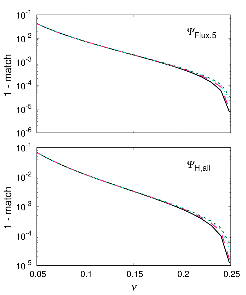
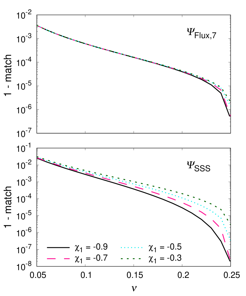
Figure 5: The mismatch ($\equiv 1-{\mathrm{match}}$) between two TaylorF2 templates with and without each phase correction due to BH absorption accumulated in the Advanced LIGO frequency band $mf\in[0.0035,\,0.018]$, where the initial total mass and spin of the large BH (labeled by ‘$2$’; $m_{2}\geq m_{1}$) are chosen to be $m=60.0M_{\odot}$ and ${\chi}_{2}=+0.90$, respectively. The results are plotted as a function of the symmetric mass ratio $\nu$ for different values of the initial anti-aligned spin of the small BH (labeled by ‘$1$’) $\chi_{1}$, and they are grouped into four panels according to what is neglected in the GW phase (1.7); Top left: the neglect of the LO horizon-flux term $\Psi^{\mathrm{F2}}_{\mathrm{Flux},5}$. Top right: the neglect of the NLO horizon-flux term $\Psi^{\mathrm{F2}}_{\mathrm{Flux},7}$. Bottom left: the neglect of all phase terms due to BH absorption $\Psi^{\mathrm{F2}}_{\mathrm{H,all}}$, including all horizon-flux terms $\Psi^{\mathrm{F2}}_{\mathrm{Flux},5}$ and $\Psi^{\mathrm{F2}}_{\mathrm{Flux},7}$ as well as the LO term due to the secular change in BH intrinsic parameters $\Psi^{\mathrm{F2}}_{\mathrm{BH},7}$. Bottom right: (for comparison) the neglect of the LO cubic-in-spin term $\Psi^{\mathrm{F2}}_{\mathrm{SSS}}$ in the non-absorption, point-particle phase term $\Psi^{\mathrm{F2}}_{\infty}$.

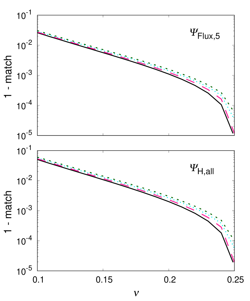
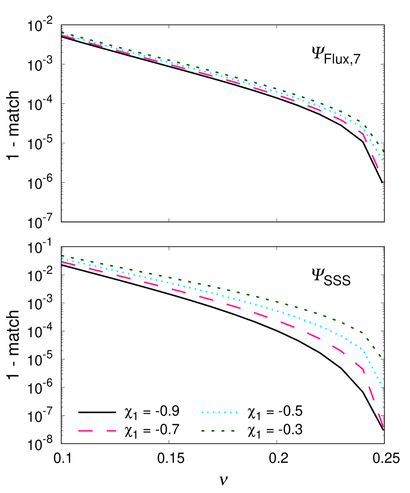
Figure 6: The mismatch ($\equiv 1-{\mathrm{match}}$) between the two TaylorF2 templates with and without each phase correction due to BH absorption accumulated in a space based detector, LISA frequency band $mf\in[2.0\times 10^{-4}\,\nu^{-3/8},\,mf_{\mathrm{ISCO}}]$, where the initial total mass and the spin of the large BH (labeled by ‘$2$’) are chosen to be $m=10^{6}M_{\odot}$ and ${\chi}_{2}=+0.90$, respectively. The results are plotted as a function of the initial symmetric mass ratio $\nu$ for different values of the initial anti-aligned spin of the small BH $\chi_{1}$. The label and grouping of the panels are the same as for figure 5.

The recent observation GW170104 [6] disfavors the aligned-spin configuration. Motivated by this measurement, the first group is concerned with BBHs with anti-aligned spins. Suppose BBH systems that have the same total-mass as those in figures 3 and 4 but have both anti aligned-spins $\chi_{1,2}=\{-0.30,\,-0.50,\,-0.70,\,-0.998\}$. We point out that mismatch for each template ${\hat{x}}_{\mathrm{T}}$ with the reference GW signal ${\tilde{h}}_{\mathrm{H}}$ for such BBHs with anti-aligned spins are smaller than that for corresponding aligned-spin BBHs with $\chi_{1,2}=\{+0.30,\,+0.50,\,+0.70,\,+0.998\}$ by the factor of $O(10)$. In fact, we find that all mismatch is below the $10^{-3}$ mark for such anti-aligned-spin BBHs. It is therefore not significant even when the BBH is in the nearly anti-extremal limit $\chi_{1,2}=-0.998$.

We also consider the mismatch between ${\tilde{x}}_{\mathrm{T}}$ and ${\tilde{h}}_{\mathrm{H}}$ for different values of initial anti-aligned spin of the small BH $\chi_{1}$ (labeled by ‘$1$’; $m_{1}\geq m_{2}$), while the spin of the large BH (labeled by ‘$2$’) is assumed to be $\chi_{2}=+0.90$, in order to explore the asymmetric, anti-aligned spin configurations. The results for such BBHs with initial total masses $m=60.0M_{\odot}$ that are observable by Advanced LIGO and for those with initial total masses $m=10^{6}M_{\odot}$ detected by LISA are summarized in figures 5 and 6, respectively. Notice that neglecting $\Psi^{\mathrm{F2}}_{\mathrm{BH},7}$ always produces the mismatch below the $10^{-5}$ mark, which are not significant for all BBHs that are considered here. For this reason, we did not plot the corresponding mismatch in these figures.

Figures 5 and 6 show that all mismatch except that from $\Psi^{\mathrm{F2}}_{\mathrm{SSS}}$ are dominated by the spin of the large BH $\chi_{2}$. The spin of the small BH $\chi_{1}$ is largely irrelevant unless BBHs are almost equal-mass configurations $\nu\gtrsim 0.22$, where none of mismatch are significant. This is an expected feature because the spin of the small BH is likely to be unimportant in the high mass-ratio regime. The mismatch from the neglect of $\Psi^{\mathrm{F2}}_{\mathrm{H,all}}$ (the cubic-in-spin phase term $\Psi^{\mathrm{F2}}_{\mathrm{SSS}}$) is therefore significant only in the high mass-ratio regime $\nu\lesssim 0.07$ ($\nu\lesssim 0.06$) for Advanced LIGO and $\nu\lesssim 0.15$ ($\nu\lesssim 0.25$) for LISA; refer back to figures 3 and 4.

The $\chi_{1}$-dependence of the match in the almost equal-mass regime, which is particularly pronounced for that from $\Psi^{\mathrm{F2}}_{\mathrm{SSS}}$, is rooted in the fact that coefficients of the term in $\Psi^{\mathrm{F2}}_{\mathrm{Flux},5},\,\Psi^{\mathrm{F2}}_{\mathrm{Flux},7}$ and $\Psi^{\mathrm{F2}}_{\mathrm{SSS}}$ that involves the anti-symmetric spin parameter $\chi_{a}$ [recall (4.6)] are not so small compared to those only proportional to the symmetric spin parameter $\chi_{s}^{3}$. In fact, the coefficient of $\chi_{a}^{2}\chi_{s}$ in $\Psi^{\mathrm{F2}}_{\mathrm{SSS}}$ are quite large $\sim O(10^{3})$ for almost equal-mass BBHs; recall (4.128). This explains why the dependence of $\chi_{1}$ is the most visible for the asymmetric spin configuration $\chi_{1}=-0.30,\,\chi_{2}=+0.90$ in the almost equal-mass regime of these figures.

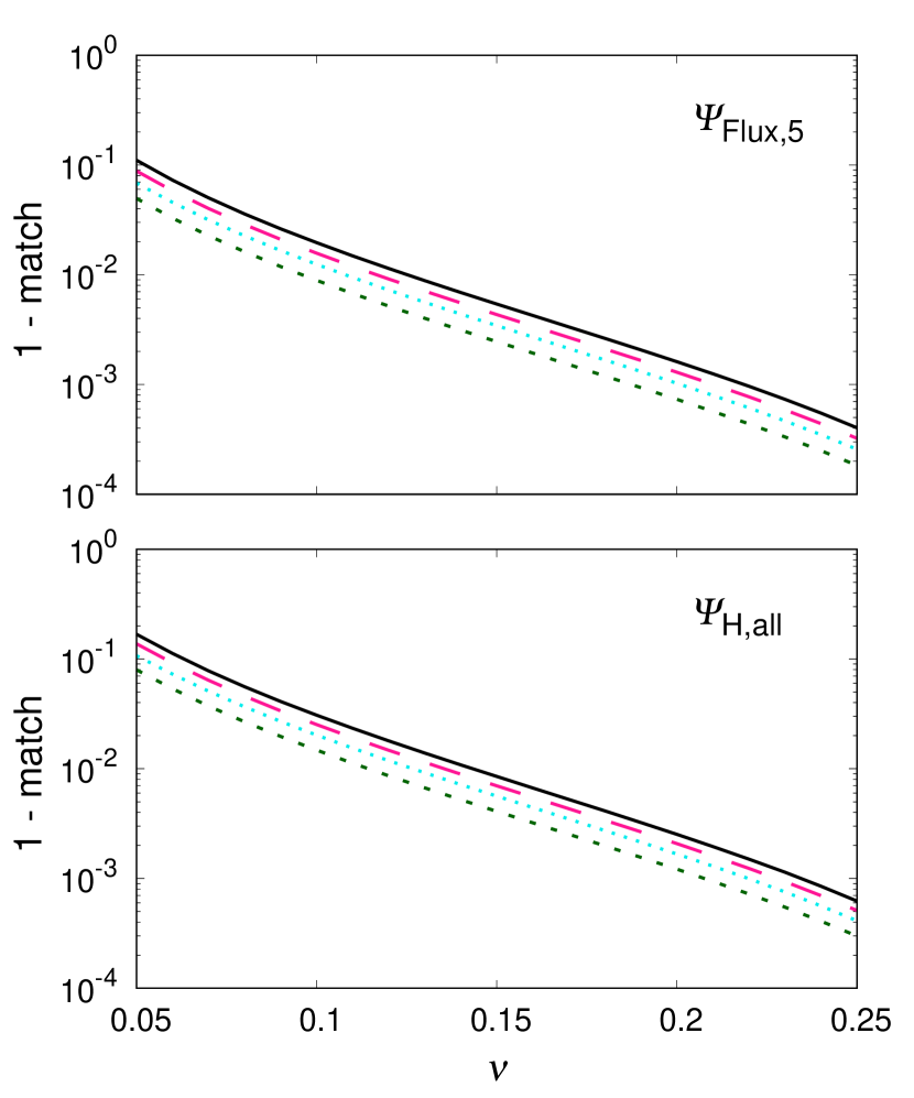
Figure 7: The mismatch ($\equiv 1-{\mathrm{match}}$) between two TaylorF2 templates with and without each phase correction due to BH absorption accumulated in the Advanced LIGO frequency band $mf\in[0.0035,\,0.018]$, where the initial aligned-spins are chosen to be near extremal values ${\chi}_{1,2}=0.998$. For $m=80.0M_{\odot}$, we set the lower cutoff frequency at $f=10.0{\mathrm{Hz}}$. The results are plotted as a function of the initial symmetric mass ratio $\nu$ for different values of the initial total mass $m_{\mathrm{tot}}\equiv m/M_{\odot}$. The label and grouping of the panels are the same as for figures 5.

The second group considers the mismatch for each template ${\tilde{x}}_{\mathrm{T}}$ with the reference signal ${\tilde{h}}_{\mathrm{H}}$ for different values of initial total masses $m$ of BBHs, while initial aligned-spins of BBHs are assumed to be $\chi_{1,2}=0.998$. The results for BBHs that are observable Advanced LIGO and LISA are summarized in figures 7 and 8, respectively. Once again, the mismatch due to the neglect of $\Psi^{\mathrm{F2}}_{\mathrm{BH},7}$ is not plotted here; the resulting mismatch is always below the $10^{-5}$ mark in both cases, and does not become significant.

Figure 7 shows that all mismatch are largely independent of the total mass; the lower total-mass system produces larger mismatch, and the plotted mismatch are different from each other only by the factor of $O(1)$. This is simply because the frequency range that we use for Advanced LIGO covers only the early inspiral phase in our analysis; recall that the upper cutoff frequency is chosen to be the relatively low frequency $mf_{\mathrm{max}}=0.018$, largely motivated by the inspiral portion of the phenomenological “PhenomD” model [44] as well as that of the NINJA project [26, 28]. For BBHs with the total mass $m/M_{\odot}=\{20.0,\,40.0,\,60.0,\,80.0\}$ considered in figure 7, the cutoff frequencies $mf_{\mathrm{min}}=0.0035$ and $mf_{\mathrm{max}}=0.018$ are translated to $f_{\mathrm{min}}\sim\{36.0,\,18.0,\,12.0,\,10.0\}$ Hz and $f_{\mathrm{max}}\sim\{183.0,\,91.0,\,61.0,\,46.0\}$ Hz, respectively; the lower cutoff frequency for $m=80.0M_{\odot}$ configuration is instead selected at $f_{\mathrm{min}}=10.0$ Hz because the noise PSD below this frequency is not well characterized. We see that none of them reaches the minimum of the Advanced LIGO’s noise PSD in (5.5), locating at $f_{\mathrm{LIGO}}\sim 250.0$ Hz. Hence, the mismatch for $m=20.0M_{\odot}$ configuration becomes largest as the frequency overlaps between ${\tilde{x}}_{\mathrm{T}}$ and ${\tilde{h}}_{\mathrm{H}}$ are in the Advanced LIGO’s wider sensitivity band (and thus have more time to accumulate a phase difference). It should be noted that our conclusion of figure 7 is therefore valid only for this specific choice of the Advanced LIGO’s frequency range.

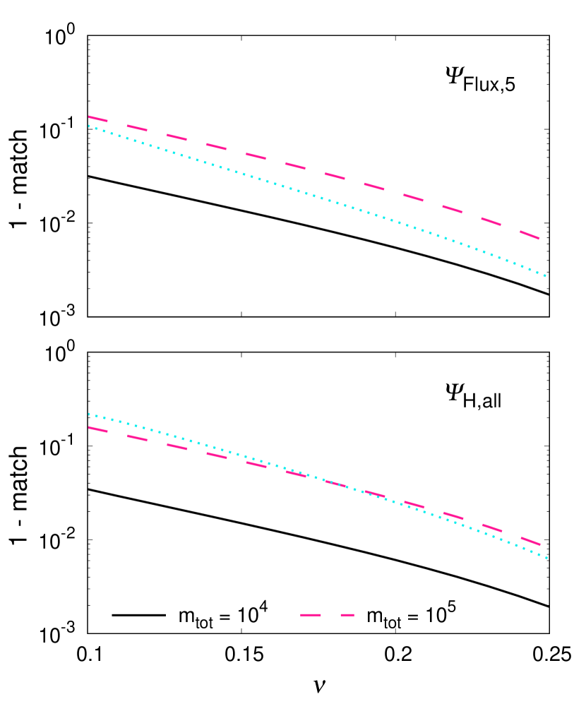
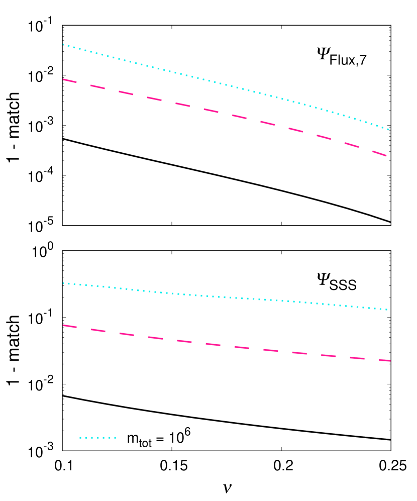
Figure 8: The mismatch ($\equiv 1-{\mathrm{match}}$) between the two TaylorF2 templates with and without each phase correction due to BH absorption accumulated in a LISA frequency band $mf\in[2.0\times 10^{-4}\,\nu^{-3/8},\,mf_{\mathrm{pole}}]$, where the initial aligned-spins are chosen to be ${\chi}_{1,2}=0.998$. Notice that the upper cutoff of the frequency is $mf_{\mathrm{pole}}$ rather than $mf_{\mathrm{ISCO}}$ to validate TaylorF2. We also set the upper cutoff frequency at $f=1.0{\mathrm{Hz}}$ for $m=10^{4}M_{\odot}$ case ($f_{\mathrm{pole}}\sim 2.2{\mathrm{Hz}}$ in this case). The label and grouping of the panels are the same as for figure 7.

Indeed, we see that the mismatch for the LISA case plotted in figure 8 shows the different dependence on the total mass $m$. For example, the mismatch from $\Psi^{\mathrm{F2}}_{\mathrm{H,all}}$ for two configurations $m=\{10^{5},10^{6}\}M_{\odot}$ are almost identical to each other (within the order-of-magnitude) and is significant in the almost equal-mass regime $\nu\lesssim 0.19$, while that for the configuration $m=10^{4}M_{\odot}$ is smaller by the factor of $O(10)$. Recall that the templates used in the LISA case is terminated near the ISCO of Kerr spacetime, including the late inspiral phase. The cutoff frequencies for the case of LISA $mf_{\mathrm{min}}=2.0\times 10^{-4}$ and $mf_{\mathrm{max}}=mf_{\mathrm{pole}}$ are approximately translated to $mf_{\mathrm{min}}\sim 6.8\times\{10^{-3},\,10^{-4},\,10^{-5}\}$ Hz and $mf_{\mathrm{max}}\sim\{1.0,\,2.2\times 10^{-1},\,2.2\times 10^{-2}\}$ Hz for the BBH with $m=\{10^{4},10^{5},10^{6}\}M_{\odot}$, respectively; the upper cutoff frequency for the $m=10^{4}M_{\odot}$ configuration is instead selected at $f_{\mathrm{max}}=1.0$ Hz because the noise PSD above this frequency may not be well characterized. Since the minimum of LISA’s noise PSD in (5.7) is at $f_{\mathrm{LISA}}\sim 8.3\times 10^{-3}$ Hz, where LISA is most sensitive to the GW signals, each configuration covers quite different frequency range of the noise PSD. The fact that the $m=10^{4}M_{\odot}$ configuration always produces the smallest mismatch is a direct consequence of this; $f_{\mathrm{LISA}}$ is only marginally covered for this configuration.

References

References

- [1] B. P. Abbott et al. [LIGO Scientific and Virgo Collaborations], Phys. Rev. Lett. 116, 061102 (2016) [arXiv:1602.03837 [gr-qc]].
- [2] B. P. Abbott et al. [LIGO Scientific and Virgo Collaborations], Phys. Rev. D 93, 122003 (2016) [arXiv:1602.03839 [gr-qc]].
- [3] B. P. Abbott et al. [LIGO Scientific and Virgo Collaborations], Phys. Rev. Lett. 116, 241102 (2016) [arXiv:1602.03840 [gr-qc]].
- [4] B. P. Abbott et al. [LIGO Scientific and Virgo Collaborations], Phys. Rev. D 93, 122004 (2016) Addendum: [Phys. Rev. D 94, 069903 (2016)] [arXiv:1602.03843 [gr-qc]].
- [5] B. P. Abbott et al. [LIGO Scientific and Virgo Collaborations], Phys. Rev. Lett. 116, 241103 (2016) [arXiv:1606.04855 [gr-qc]].
- [6] B. P. Abbott et al. [LIGO Scientific and VIRGO Collaborations], Phys. Rev. Lett. 118, 22, 221101 (2017) doi:10.1103/PhysRevLett.118.221101 [arXiv:1706.01812 [gr-qc]].
- [7] B. P. Abbott et al. [LIGO Scientific and Virgo Collaborations], Phys. Rev. Lett. 119, 141101 (2017).
- [8] B. P. Abbott et al. [LIGO Scientific and Virgo Collaborations], Phys. Rev. X 6, 041015 (2016) [arXiv:1606.04856 [gr-qc]].
- [9] B. P. Abbott et al. [LIGO Scientific and Virgo Collaborations], Phys. Rev. Lett. 116, 131103 (2016) [arXiv:1602.03838 [gr-qc]].
- [10] B. P. Abbott et al. [LIGO Scientific and Virgo Collaborations], Class. Quant. Grav. 33, 134001 (2016) [arXiv:1602.03844 [gr-qc]].
- [11] B. P. Abbott et al. [LIGO Scientific Collaboration], arXiv:1602.03845 [gr-qc].
- [12] B. P. Abbott et al. [LIGO Scientific and VIRGO Collaborations], Living Rev. Rel. 19, 1 (2016) [arXiv:1304.0670 [gr-qc]].
- [13] K. Somiya [KAGRA Collaboration], Class. Quant. Grav. 29, 124007 (2012) [arXiv:1111.7185 [gr-qc]].
- [14] Y. Aso et al. [KAGRA Collaboration], Phys. Rev. D 88, 043007 (2013) [arXiv:1306.6747 [gr-qc]].
- [15] P. Amaro-Seoane et al., arXiv:1702.00786 [astro-ph.IM].
- [16] N. Seto, S. Kawamura and T. Nakamura, Phys. Rev. Lett. 87, 221103 (2001), [astro-ph/0108011].
- [17] S. Sato, “Space Gravitational Wave Observatory,” (2016), presented at JPS 2016 Autumn Meeting, University of Miyazaki.
- [18] B. Allen, W. G. Anderson, P. R. Brady, D. A. Brown and J. D. E. Creighton, Phys. Rev. D 85, 122006 (2012) [gr-qc/0509116].
- [19] E. Poisson and C. M. Will, Gravity: Newtonian, Post-Newtonian, Relativistic, (Cambridge University Press, 2014).
- [20] L. Blanchet, Living Rev. Rel. 17, 2 (2014) [arXiv:1310.1528 [gr-qc]].
- [21] F. Pretorius, Phys. Rev. Lett. 95, 121101 (2005) [gr-qc/0507014].
- [22] M. Campanelli, C. O. Lousto, P. Marronetti and Y. Zlochower, Phys. Rev. Lett. 96, 111101 (2006) [gr-qc/0511048].
- [23] J. G. Baker, J. Centrella, D. I. Choi, M. Koppitz and J. van Meter, Phys. Rev. Lett. 96, 111102 (2006) [gr-qc/0511103].
- [24] B. Aylott et al., Class. Quant. Grav. 26, 165008 (2009) [arXiv:0901.4399 [gr-qc]].
- [25] B. Aylott et al., Class. Quant. Grav. 26, 114008 (2009) [arXiv:0905.4227 [gr-qc]].
- [26] P. Ajith et al., Class. Quant. Grav. 29 (2012) 124001 Addendum: [Class. Quant. Grav. 30 (2013) 199401] [arXiv:1201.5319 [gr-qc]].
- [27] I. Hinder et al., Class. Quant. Grav. 31, 025012 (2014) [arXiv:1307.5307 [gr-qc]].
- [28] J. Aasi et al. [LIGO Scientific and VIRGO and NINJA-2 Collaborations], Class. Quant. Grav. 31, 115004 (2014) [arXiv:1401.0939 [gr-qc]].
- [29] G. Lovelace et al., Class. Quant. Grav. 33, 244002 (2016) [arXiv:1607.05377 [gr-qc]].
- [30] A. Buonanno and T. Damour, Phys. Rev. D 59, 084006 (1999) [gr-qc/9811091].
- [31] A. Buonanno and T. Damour, Phys. Rev. D 62 (2000) 064015 [gr-qc/0001013].
- [32] T. Damour, P. Jaranowski and G. Schaefer, Phys. Rev. D 78, 024009 (2008) [arXiv:0803.0915 [gr-qc]].
- [33] T. Damour and A. Nagar, Phys. Rev. D 79, 081503 (2009) [arXiv:0902.0136 [gr-qc]].
- [34] E. Barausse and A. Buonanno, Phys. Rev. D 81, 084024 (2010) [arXiv:0912.3517 [gr-qc]].
- [35] A. Taracchini et al., Phys. Rev. D 89, 061502 (2014) [arXiv:1311.2544 [gr-qc]].
- [36] T. Damour and A. Nagar, Phys. Rev. D 90, 044018 (2014) [arXiv:1406.6913 [gr-qc]].
- [37] A. Bohé et al., Phys. Rev. D 95, 044028 (2017) [arXiv:1611.03703 [gr-qc]].
- [38] Y. Pan, A. Buonanno, J. G. Baker, J. Centrella, B. J. Kelly, S. T. McWilliams, F. Pretorius and J. R. van Meter, Phys. Rev. D 77, 024014 (2008) [arXiv:0704.1964 [gr-qc]].
- [39] P. Ajith et al., Phys. Rev. D 77, 104017 (2008) Erratum: [Phys. Rev. D 79, 129901 (2009)] [arXiv:0710.2335 [gr-qc]].
- [40] P. Ajith et al., Phys. Rev. Lett. 106, 241101 (2011) [arXiv:0909.2867 [gr-qc]].
- [41] L. Santamaria et al., Phys. Rev. D 82, 064016 (2010) [arXiv:1005.3306 [gr-qc]].
- [42] M. Hannam, P. Schmidt, A. Bohé, L. Haegel, S. Husa, F. Ohme, G. Pratten and M. Pürrer, Phys. Rev. Lett. 113, 151101 (2014) [arXiv:1308.3271 [gr-qc]].
- [43] S. Husa, S. Khan, M. Hannam, M. PÜrrer, F. Ohme, X. Jiménez Forteza and A. Bohé, Phys. Rev. D 93, 044006 (2016) [arXiv:1508.07250 [gr-qc]].
- [44] S. Khan, S. Husa, M. Hannam, F. Ohme, M. Pürrer, X. Jiménez Forteza and A. Bohé, Phys. Rev. D 93, 044007 (2016) [arXiv:1508.07253 [gr-qc]].
- [45] B. P. Abbott et al. [LIGO Scientific and Virgo Collaborations], Phys. Rev. Lett. 116, 221101 (2016) [arXiv:1602.03841 [gr-qc]].
- [46] B. P. Abbott et al. [LIGO Scientific and Virgo Collaborations], Phys. Rev. D 94, 064035 (2016) [arXiv:1606.01262 [gr-qc]].
- [47] B. P. Abbott et al. [LIGO Scientific and Virgo Collaborations], Astrophys. J. 833, L1 (2016) [arXiv:1602.03842 [astro-ph.HE]].
- [48] B. P. Abbott et al. [LIGO Scientific and Virgo Collaborations], Astrophys. J. 818, L22 (2016) [arXiv:1602.03846 [astro-ph.HE]].
- [49] B. P. Abbott et al. [LIGO Scientific and Virgo Collaborations], Phys. Rev. Lett. 116, 131102 (2016) [arXiv:1602.03847 [gr-qc]].
- [50] B. P. Abbott et al. [LIGO Scientific and Virgo and ASKAP and BOOTES and DES and DEC and Fermi GBM and Fermi-LAT and GRAWITA and INTEGRAL and iPTF and InterPlanetary Network and J-GEM and La Silla-QUEST Survey and Liverpool Telescope and LOFAR and MASTER and MAXI and MWA and Pan-STARRS and PESSTO and Pi of the Sky and SkyMapper and Swift and C2PU and TOROS and VISTA Collaborations], Astrophys. J. 826, L13 (2016) [arXiv:1602.08492 [astro-ph.HE]].
- [51] B. P. Abbott et al. [LIGO Scientific and Virgo and ASKAP and BOOTES and DES and DEC and Fermi-GBM and Fermi-LAT and GRAWITA and INTEGRAL and iPTF and InterPlanetary Network and J-GEM and La Silla-QUEST Survey and Liverpool Telescope and LOFAR and MASTER and MAXI and MWA and Pan-STARRS and PESSTO and Pi of the Sky and SkyMapper and Swift and TAROT and Zadko and Algerian National Observatory and C2PU and TOROS and VISTA Collaborations], Astrophys. J. Suppl. 225, 8 (2016) [arXiv:1604.07864 [astro-ph.HE]].
- [52] P. C. Peters and J. Mathews, Phys. Rev. 131, 435 (1963).
- [53] P. C. Peters, Phys. Rev. 136, B1224 (1964).
- [54] C. K. Mishra, A. Kela, K. G. Arun and G. Faye, Phys. Rev. D 93, 084054 (2016) [arXiv:1601.05588 [gr-qc]].
- [55] H. Bondi, M. G. J. van der Burg and A. W. K. Metzner, Proc. Roy. Soc. Lond. A 269, 21 (1962).
- [56] R. K. Sachs, Proc. Roy. Soc. Lond. A 270, 103 (1962).
- [57] K. Alvi, Phys. Rev. D 64, 104020 (2001) [gr-qc/0107080].
- [58] E. Poisson, Phys. Rev. D 70, 084044 (2004) [gr-qc/0407050].
- [59] A. Nagar and S. Akcay, Phys. Rev. D 85, 044025 (2012) [arXiv:1112.2840 [gr-qc]].
- [60] K. Chatziioannou, E. Poisson and N. Yunes, Phys. Rev. D 87, 044022 (2013) [arXiv:1211.1686 [gr-qc]].
- [61] A. Taracchini, A. Buonanno, S. A. Hughes and G. Khanna, Phys. Rev. D 88, 044001 (2013) Erratum: [Phys. Rev. D 88, 109903 (2013)] [arXiv:1305.2184 [gr-qc]].
- [62] K. Chatziioannou, E. Poisson and N. Yunes, Phys. Rev. D 94, 084043 (2016) [arXiv:1608.02899 [gr-qc]].
- [63] Y. Mino, M. Sasaki and T. Tanaka, Prog. Theor. Phys. Suppl. 128, 373 (1997) [gr-qc/9712056].
- [64] M. Sasaki and H. Tagoshi, Living Rev. Rel. 6, 6 (2003) [gr-qc/0306120].
- [65] R. Fujita, PTEP 2015, 033E01 (2015) [arXiv:1412.5689 [gr-qc]].
- [66] E. Poisson and M. Sasaki, Phys. Rev. D 51, 5753 (1995) [gr-qc/9412027].
- [67] S. Marsat, Class. Quant. Grav. 32, 085008 (2015) [arXiv:1411.4118 [gr-qc]].
- [68] H. Tagoshi, S. Mano and E. Takasugi, Prog. Theor. Phys. 98, 829 (1997) [gr-qc/9711072].
- [69] S. A. Hughes, Phys. Rev. D 64, 064004 (2001) Erratum: [Phys. Rev. D 88, 109902 (2013)] [gr-qc/0104041].
- [70] N. Yunes, A. Buonanno, S. A. Hughes, M. Coleman Miller and Y. Pan, Phys. Rev. Lett. 104, 091102 (2010) [arXiv:0909.4263 [gr-qc]].
- [71] N. Yunes, A. Buonanno, S. A. Hughes, Y. Pan, E. Barausse, M. C. Miller and W. Throwe, Phys. Rev. D 83, 044044 (2011) Erratum: [Phys. Rev. D 88, 10, 109904 (2013)] [arXiv:1009.6013 [gr-qc]].
- [72] M. Hannam, S. Husa, B. Bruegmann and A. Gopakumar, Phys. Rev. D 78, 104007 (2008) [arXiv:0712.3787 [gr-qc]].
- [73] M. Hannam, S. Husa, F. Ohme, D. Muller and B. Bruegmann, Phys. Rev. D 82, 124008 (2010) [arXiv:1007.4789 [gr-qc]].
- [74] A. Maselli, P. Pani, V. Cardoso, T. Abdelsalhin, L. Gualtieri and V. Ferrari, arXiv:1703.10612 [gr-qc].
- [75] T. Damour, B. R. Iyer and B. S. Sathyaprakash, Phys. Rev. D 63, 044023 (2001) Erratum: [Phys. Rev. D 72, 029902 (2005)] [gr-qc/0010009].
- [76] T. Damour, B. R. Iyer and B. S. Sathyaprakash, Phys. Rev. D 66, 027502 (2002) [gr-qc/0207021].
- [77] K. G. Arun, B. R. Iyer, B. S. Sathyaprakash and P. A. Sundararajan, Phys. Rev. D 71, 084008 (2005) Erratum: [Phys. Rev. D 72, 069903 (2005)] [gr-qc/0411146].
- [78] A. Buonanno, B. Iyer, E. Ochsner, Y. Pan and B. S. Sathyaprakash, Phys. Rev. D 80, 084043 (2009) [arXiv:0907.0700 [gr-qc]].
- [79] V. Varma, R. Fujita, A. Choudhary and B. R. Iyer, Phys. Rev. D 88, 024038 (2013) [arXiv:1304.5675 [gr-qc]].
- [80] K. G. Arun, A. Buonanno, G. Faye and E. Ochsner, Phys. Rev. D 79, 104023 (2009) Erratum: [Phys. Rev. D 84, 049901 (2011)] [arXiv:0810.5336 [gr-qc]].
- [81] M. Wade, J. D. E. Creighton, E. Ochsner and A. B. Nielsen, Phys. Rev. D 88, 083002 (2013) [arXiv:1306.3901 [gr-qc]].
- [82] A. H. Mroue et al., Phys. Rev. Lett. 111, 24, 241104 (2013) [arXiv:1304.6077 [gr-qc]].
- [83] K. Jani, J. Healy, J. A. Clark, L. London, P. Laguna and D. Shoemaker, Class. Quant. Grav. 33, 20, 204001 (2016) [arXiv:1605.03204 [gr-qc]].
- [84] J. Healy, C. O. Lousto, Y. Zlochower and M. Campanelli, Class. Quant. Grav. 34, 22, 224001 (2017) [arXiv:1703.03423 [gr-qc]].
- [85] A. H. Nitz, A. Lundgren, D. A. Brown, E. Ochsner, D. Keppel and I. W. Harry, Phys. Rev. D 88, 124039 (2013) [arXiv:1307.1757 [gr-qc]].
- [86] K. S. Thorne, Astrophys. J. 191, 507 (1974).
- [87] J. M. Bardeen, W. H. Press and S. A. Teukolsky, Astrophys. J. 178, 347 (1972).
- [88] E. Berti, A. Buonanno and C. M. Will, Phys. Rev. D 71, 084025 (2005) [gr-qc/0411129].
- [89] N. Yunes and E. Berti, Phys. Rev. D 77, 124006 (2008) Erratum: [Phys. Rev. D 83, 109901 (2011)] [arXiv:0803.1853 [gr-qc]].
- [90] Z. Zhang, N. Yunes and E. Berti, Phys. Rev. D 84, 024029 (2011) [arXiv:1103.6041 [gr-qc]].
- [91] N. Sago, R. Fujita and H. Nakano, Phys. Rev. D 93, 104023 (2016) [arXiv:1601.02174 [gr-qc]].
- [92] R. Fujita, N. Sago and H. Nakano, Class. Quant. Grav. 35, 2, 027001 (2018) [arXiv:1707.09309 [gr-qc]].
- [93] B. J. Owen, Phys. Rev. D 53, 6749 (1996) [gr-qc/9511032].
- [94] B. J. Owen and B. S. Sathyaprakash, Phys. Rev. D 60, 022002 (1999) [gr-qc/9808076].
- [95] T. Damour, B. R. Iyer and B. S. Sathyaprakash, Phys. Rev. D 57, 885 (1998) [gr-qc/9708034].
- [96] G. M. Harry [LIGO Scientific Collaboration], Class. Quant. Grav. 27, 084006 (2010).
- [97] S. Babak et al., Phys. Rev. D 95, 10, 103012 (2017) [arXiv:1703.09722 [gr-qc]].
- [98] M. Armano et al., Phys. Rev. Lett. 116, 23, 231101 (2016).
- [99] J. Calderón Bustillo, P. Laguna and D. Shoemaker, Phys. Rev. D 95, 10, 104038 (2017) [arXiv:1612.02340 [gr-qc]].
- [100] A. R. Williamson, J. Lange, R. O’Shaughnessy, J. A. Clark, P. Kumar, J. Calderón Bustillo and J. Veitch, arXiv:1709.03095 [gr-qc].
- [101] V. Varma, P. Ajith, S. Husa, J. C. Bustillo, M. Hannam and M. Pürrer, Phys. Rev. D 90, 12, 124004 (2014) [arXiv:1409.2349 [gr-qc]].
- [102] V. Varma and P. Ajith, arXiv:1612.05608 [gr-qc].
- [103] L. London et al., arXiv:1708.00404 [gr-qc].
- [104] K. Yagi and N. Yunes, Phys. Rev. D 89, 021303 (2014) [arXiv:1310.8358 [gr-qc]].
- [105] K. Yagi, Phys. Rev. D 89, 043011 (2014) [arXiv:1311.0872 [gr-qc]].
- [106] M. Favata, Phys. Rev. Lett. 112, 101101 (2014) [arXiv:1310.8288 [gr-qc]].
- [107] P. Kumar et al., Phys. Rev. D 93, 10, 104050 (2016) [arXiv:1601.05396 [gr-qc]].
- [108] B. P. Abbott et al. [LIGO Scientific and Virgo Collaborations], Class. Quant. Grav. 34, 10, 104002 (2017) [arXiv:1611.07531 [gr-qc]].
- [109] A. Bohé, G. Faye, S. Marsat and E. K. Porter, Class. Quant. Grav. 32, 195010 (2015) [arXiv:1501.01529 [gr-qc]].
- [110] T. Damour, P. Jaranowski and G. Schäfer, Phys. Rev. D 89, 064058 (2014) [arXiv:1401.4548 [gr-qc]].
- [111] T. Damour, P. Jaranowski and G. Schäfer, Phys. Rev. D 93, 084014 (2016) [arXiv:1601.01283 [gr-qc]].
- [112] L. Bernard, L. Blanchet, A. Bohé, G. Faye and S. Marsat, Phys. Rev. D 95, 044026 (2017) [arXiv:1610.07934 [gr-qc]].
- [113] S. Marsat, A. Bohé, L. Blanchet and A. Buonanno, Class. Quant. Grav. 31, 025023 (2014) [arXiv:1307.6793 [gr-qc]].
- [114] T. Tanaka, Y. Mino, M. Sasaki and M. Shibata, Phys. Rev. D 54, 3762 (1996) [gr-qc/9602038].
- [115] F. Messina and A. Nagar, Phys. Rev. D 95, 12, 124001 (2017) Erratum: [Phys. Rev. D 96, 4, 049907 (2017)] [arXiv:1703.08107 [gr-qc]].
- [116] N. Sago and R. Fujita, in preparation.
- [117] H. Tagoshi, M. Shibata, T. Tanaka and M. Sasaki, Phys. Rev. D 54, 1439 (1996) [gr-qc/9603028].
- [118] S. Isoyama, R. Fujita, N. Sago, H. Tagoshi and T. Tanaka, Phys. Rev. D 87, 024010 (2013) [arXiv:1210.2569 [gr-qc]].
- [119] W. B. Han, Phys. Rev. D 82, 084013 (2010) [arXiv:1008.3324 [gr-qc]].
- [120] E. Harms, G. Lukes-Gerakopoulos, S. Bernuzzi and A. Nagar, Phys. Rev. D 93, 4, 044015 (2016) [arXiv:1510.05548 [gr-qc]].
- [121] M. A. Scheel, M. Giesler, D. A. Hemberger, G. Lovelace, K. Kuper, M. Boyle, B. Szilágyi and L. E. Kidder, Class. Quant. Grav. 32, 105009 (2015) [arXiv:1412.1803 [gr-qc]].
- [122] C. O. Lousto, private communication.
- [123] T. Futamase and Y. Itoh, Living Rev. Rel. 10, 2 (2007).
- [124] A. Le Tiec, L. Blanchet and B. F. Whiting, Phys. Rev. D 85, 064039 (2012) [arXiv:1111.5378 [gr-qc]].
- [125] L. Blanchet, Phys. Rev. D 55, 714 (1997) [gr-qc/9609049].
- [126] T. Chu, H. P. Pfeiffer and M. A. Scheel, Phys. Rev. D 80, 124051 (2009) [arXiv:0909.1313 [gr-qc]].
- [127] T. Damour, A. Nagar, D. Pollney and C. Reisswig, Phys. Rev. Lett. 108, 131101 (2012) [arXiv:1110.2938 [gr-qc]].
- [128] A. Le Tiec, E. Barausse and A. Buonanno, Phys. Rev. Lett. 108, 131103 (2012) [arXiv:1111.5609 [gr-qc]].
- [129] A. Nagar, T. Damour, C. Reisswig and D. Pollney, Phys. Rev. D 93, no. 4, 044046 (2016) [arXiv:1506.08457 [gr-qc]].
- [130] A. Gopakumar, arXiv:0712.3236 [gr-qc].
- [131] A. Gopakumar, M. Hannam, S. Husa and B. Bruegmann, Phys. Rev. D 78, 064026 (2008) [arXiv:0712.3737 [gr-qc]].
- [132] S. Bose, A. Gopakumar and M. Tessmer, arXiv:0807.2400 [gr-qc].
- [133] Y. Pan, A. Buonanno, R. Fujita, E. Racine and H. Tagoshi, Phys. Rev. D 83, 064003 (2011) Erratum: [Phys. Rev. D 87, 109901 (2013)] [arXiv:1006.0431 [gr-qc]].
- [134] A. Nagar and A. Shah, Phys. Rev. D 94, 104017 (2016) [arXiv:1606.00207 [gr-qc]].
- [135] A. Buonanno, Y. b. Chen and M. Vallisneri, Phys. Rev. D 67, 104025 (2003) Erratum: [Phys. Rev. D 74, 029904 (2006)] [gr-qc/0211087].
- [136] P. Ajith, Phys. Rev. D 84, 084037 (2011) [arXiv:1107.1267 [gr-qc]].
- [137] L. Blanchet, B. R. Iyer, C. M. Will and A. G. Wiseman, Class. Quant. Grav. 13, 575 (1996) [gr-qc/9602024].
- [138] L. Blanchet, G. Faye, B. R. Iyer and S. Sinha, Class. Quant. Grav. 25, 165003 (2008) Erratum: [Class. Quant. Grav. 29, 239501 (2012)] [arXiv:0802.1249 [gr-qc]].
- [139] A. Buonanno, G. Faye and T. Hinderer, Phys. Rev. D 87, 044009 (2013) [arXiv:1209.6349 [gr-qc]].
- [140] L. Blanchet, A. Buonanno and G. Faye, Phys. Rev. D 84, 064041 (2011) [arXiv:1104.5659 [gr-qc]].
- [141] G. Faye, S. Marsat, L. Blanchet and B. R. Iyer, Class. Quant. Grav. 29, 175004 (2012) [arXiv:1204.1043 [gr-qc]].
- [142] G. Faye, L. Blanchet and B. R. Iyer, Class. Quant. Grav. 32, 045016 (2015) [arXiv:1409.3546 [gr-qc]].
- [143] T. Marchand, L. Blanchet and G. Faye, Class. Quant. Grav. 33, 244003 (2016) [arXiv:1607.07601 [gr-qc]].
- [144] S. Bose, B. Hall, N. Mazumder, S. Dhurandhar, A. Gupta and A. Lundgren, J. Phys. Conf. Ser. 716, 1, 012007 (2016) [arXiv:1602.02621 [astro-ph.IM]].
- [145] B. Allen, Phys. Rev. D 71, 062001 (2005) [gr-qc/0405045].
- [146] C. Cutler and E. E. Flanagan, Phys. Rev. D 49, 2658 (1994) [gr-qc/9402014].
- [147] B. S. Sathyaprakash, Phys. Rev. D 50, 12, R7111 (1994) [gr-qc/9411043].
- [148] T. A. Apostolatos, Phys. Rev. D 52, 605 (1995).
- [149] A. Samajdar and K. G. Arun, Phys. Rev. D 96, 10, 104027 (2017) [arXiv:1708.00671 [gr-qc]].
- [150] C. Cutler, Phys. Rev. D 57, 7089 (1998) [gr-qc/9703068].
- [151] P. L. Bender and D. Hils, Class. Quant. Grav. 14, 1439 (1997).
- [152] S. T. McWilliams, B. J. Kelly and J. G. Baker, Phys. Rev. D 82, 024014 (2010) [arXiv:1004.0961 [gr-qc]].