Superuniversal transport near a $(2+1)$-dimensional quantum critical point

Abstract

We compute the zero-temperature conductivity in the two-dimensional quantum O($N$) model using a nonperturbative functional renormalization-group approach. At the quantum critical point we find a universal conductivity $\sigma^{*}/\sigma_{Q}$ (with $\sigma_{Q}=q^{2}/h$ the quantum of conductance and $q$ the charge) in reasonable quantitative agreement with quantum Monte Carlo simulations and conformal bootstrap results. In the ordered phase the conductivity tensor is defined, when $N\geq 3$, by two independent elements, $\sigma_{\rm A}(\omega)$ and $\sigma_{\rm B}(\omega)$, respectively associated with SO($N$) rotations which do and do not change the direction of the order parameter. Whereas $\sigma_{\rm A}(\omega\to 0)$ corresponds to the response of a superfluid (or perfect inductance), the numerical solution of the flow equations shows that $\lim_{\omega\to 0}\sigma_{\rm B}(\omega)/\sigma_{Q}=\sigma_{\rm B}^{*}/\sigma_{Q}$ is a superuniversal (i.e. $N$-independent) constant. These numerical results, as well as the known exact value $\sigma_{\rm B}^{*}/\sigma_{Q}=\pi/8$ in the large-$N$ limit, allow us to conjecture that $\sigma_{\rm B}^{*}/\sigma_{Q}=\pi/8$ holds for all values of $N$, a result that can be understood as a consequence of gauge invariance and asymptotic freedom of the Goldstone bosons in the low-energy limit.

Introduction. Understanding the physical properties of a system near a quantum phase transition constitutes an important problem in condensed-matter physics. This is particularly true of transport properties since strong fluctuations near the quantum critical point (QCP) often lead to the absence of well-defined quasi-particles and the breakdown of perturbation many-body theory.Sachdev (2011)

In this Rapid Communication, we discuss the zero-temperature coherent transport near a relativistic $(2+1)$-dimensional QCP with an O($N$)-symmetric order parameter. We use a nonperturbative functional renormalization-group (NPRG) approach to compute the frequency-dependent conductivity in the quantum O($N$) model. The latter describes many condensed-matter systems with a relativistic effective low-energy dynamics: quantum antiferromagnets, bosons in optical lattices, Josephson junctions, etc. At the QCP we find a universal conductivityFisher et al. (1990); not $\sigma^{*}/\sigma_{Q}$ (with $\sigma_{Q}=q^{2}/h$ the quantum of conductance and $q$ the charge) in reasonable quantitative agreement with quantum Monte Carlo simulationsWitczak-Krempa et al. (2014); Chen et al. (2014); Gazit et al. (2013); Katz et al. (2014); Gazit et al. (2014) and conformal bootstrap results.Kos et al. (2015) Our main result concerns the broken-symmetry phase, where the conductivity tensor has two independent elements $\sigma_{\rm A}$ and $\sigma_{\rm B}$ when $N\geq 3$, respectively associated with SO($N$) rotations which do and do not change the direction of the order parameter. Whereas $\sigma_{\rm A}(\omega\to 0)$ corresponds to the response of a superfluid (or perfect inductance), the numerical solution of the NPRG equations together with the exact large-$N$ result leads us to conjecture that $\sigma_{\rm B}(\omega\to 0)/\sigma_{Q}$ takes the superuniversal (i.e. $N$-independent) value $\sigma_{\rm B}^{*}/\sigma_{Q}=\pi/8$. We argue that this result is a consequence of gauge (rotation) invariance and asymptotic freedom in the infrared, i.e. the fact that Goldstone bosons become effectively noninteracting in the low-energy limit.

This conjecture has been anticipated in Ref. Rose and Dupuis, 2017 using an approximate solution of the NPRG equations based on a derivative expansion of the scale-dependent effective action. However, because of infrared singularities which invalidate the derivative expansion at low energy, we could not obtain definite values for $\sigma^{*}/\sigma_{Q}$ and $\sigma_{\rm B}^{*}/\sigma_{Q}$. Here we report results obtained from a different approximation of the NPRG equations which does not suffer from these limitations.

While universality is a generic consequence of the proximity of the QCP, universal quantities (e.g. critical exponents or scaling functions) in general depend on $N$. To our knowledge there are very few exceptions. The critical energy densities of O($N$) models on a $d$-dimensional lattice with long-range interactions are known to be all equal to the one of the Ising model.Campa et al. (2003) The same is true for all O($N$) models on a one-dimensional lattice with nearest-neighbor interactions. It has been conjecturedCasetti et al. (2011) that this superuniversality should hold for all $d$-dimensional O($N$) models but a firm numerical confirmation has not been provided so far.Nerattini et al. (2014)

Quantum O($N$) model and NPRG approach. The two-dimensional quantum O($N$) model is defined by the Euclidean action

$$S=\int_{\bf x}\biggl{\{}\frac{1}{2}\sum_{\mu=0,x,y}({\partial_{\mu}}\boldsymbol{\varphi})^{2}+\frac{r_{0}}{2}\boldsymbol{\varphi}^{2}+\frac{u_{0}}{4!N}{(\boldsymbol{\varphi}^{2})}^{2}\biggr{\}},$$ (1)

where we use the notation ${\bf x}=({\bf r},\tau)$, $\int_{\bf x}=\int_{0}^{\beta}d\tau\int d^{2}r$ and $\partial_{0}={\partial_{\tau}}$. $\boldsymbol{\varphi}({\bf x})$ is an $N$-component real field, ${\bf r}$ a two-dimensional coordinate, $\tau\in[0,\beta]$ an imaginary time, and $\beta=1/T$ the inverse temperature (we set $\hbar=k_{B}=1$). $r_{0}$ and $u_{0}$ are temperature-independent coupling constants and the (bare) velocity of the $\boldsymbol{\varphi}$ field has been set to unity. The model is regularized by an ultraviolet cutoff $\Lambda$. Assuming $u_{0}$ fixed, there is a quantum phase transition between a disordered phase ($r_{0}>r_{0c}$) and an ordered phase ($r_{0}<r_{0c}$) where the O($N$) symmetry is spontaneously broken. The QCP at $r_{0}=r_{0c}$ is in the universality class of the three-dimensional classical O($N$) model and the phase transition is governed by the three-dimensional Wilson-Fisher fixed point.

In the following we consider only the zero-temperature limit where the two-dimensional quantum model is equivalent to the three-dimensional classical model. We thus identify $\tau$ with a third spatial dimension so that ${\bf x}=({\bf r},\tau)\equiv(x,y,z)$. A correlation function $\chi(p_{x},p_{y},p_{z})$ computed in the classical model then corresponds to the correlation function $\chi(p_{x},p_{y},i\omega_{n})$ of the quantum model, with $\omega_{n}\equiv p_{z}$ a bosonic Matsubara frequency, and yields the retarded dynamical correlation function $\chi^{R}(p_{x},p_{y},\omega)$ after analytical continuation $i\omega_{n}\to\omega+i0^{+}$.

The O($N$) symmetry of the action (1) implies the conservation of the total angular momentum and the existence of a conserved current. To compute the associated conductivity, we include in the model an external non-Abelian gauge field $A_{\mu}=A_{\mu}^{a}T^{a}$ (with an implicit sum over repeated discrete indices), where $\{T^{a}\}$ denotes a set of SO($N$) generators (made of $N(N-1)/2$ linearly independent skew-symmetric matrices). This amounts to replacing the derivative ${\partial_{\mu}}$ in Eq. (1) by the covariant derivative $D_{\mu}={\partial_{\mu}}-qA_{\mu}$ (we set the charge $q$ equal to unity in the following and restore it, as well as $\hbar$, whenever necessary). This makes the action (1) invariant in the local gauge transformation $\boldsymbol{\varphi}^{\prime}=O\boldsymbol{\varphi}$ and $A_{\mu}^{\prime}=OA_{\mu}O^{T}+({\partial_{\mu}}O)O^{T}$ where $O$ is a space-dependent SO($N$) rotation. The current density $J^{a}_{\mu}({\bf x})=-\delta S/\delta A^{a}_{\mu}({\bf x})$ is then expressed as Rose and Dupuis (2017)

$$J^{a}_{\mu}=j^{a}_{\mu}-A_{\mu}\boldsymbol{\varphi}\cdot T^{a}\boldsymbol{\varphi},\quad j^{a}_{\mu}={\partial_{\mu}}\boldsymbol{\varphi}\cdot T^{a}\boldsymbol{\varphi},$$ (2)

where $j^{a}_{\mu}$ denotes the “paramagnetic” part. For $N=2$, there is a single generator $T$, which can be chosen as minus the antisymmetric tensor $\epsilon_{ij}$,Rose and Dupuis (2017) and we recover the standard expression $j_{\mu}=-i[\psi^{*}{\partial_{\mu}}\psi-({\partial_{\mu}}\psi^{*})\psi]$ of the current density of bosons described by a complex field $\psi=(\varphi_{1}+i\varphi_{2})/\sqrt{2}$. For $N=3$, there are three generators $-iS^{1}$, $-iS^{2}$ and $-iS^{3}$ related to spin-one matrices $S^{i}$. One then finds $j_{\mu}^{i}=-\epsilon_{ijk}({\partial_{\mu}}\varphi_{j})\varphi_{k}$ ($\epsilon_{ijk}$ is the antisymmetric tensor) in agreement with the continuum limit of spin currents defined in lattice models.[See; e.g.; ]Rueckriegel17

The frequency-dependent conductivity of the quantum model is defined as the linear response to the gauge field, i.e.

$$\sigma^{ab}_{\mu\nu}(\omega)=-\frac{i}{(\omega+i0^{+})}K^{ab}_{\mu\nu}{}^{R}(\omega).$$ (3)

$K^{R}$ is the retarded part of the correlation function

$$K^{ab}_{\mu\nu}(i\omega_{n})=\Pi^{ab}_{\mu\nu}(i\omega_{n})-\delta_{\mu\nu}\langle T^{a}\boldsymbol{\varphi}\cdot T^{b}\boldsymbol{\varphi}\rangle,$$ (4)

where we have set the momentum to zero and $\Pi^{ab}_{\mu\nu}=\langle j^{a}_{\mu}j^{b}_{\nu}\rangle$ is the paramagnetic current-current correlation function. The conductivity having a vanishing scaling dimension in two space dimensions, it satisfiesFisher et al. (1990); Damle and Sachdev (1997)

$$\sigma^{ab}_{\mu\nu}(\omega)=\sigma_{Q}\Sigma^{ab}_{\mu\nu}{}_{\pm}\left(\frac{\omega+i0^{+}}{\Delta}\right),$$ (5)

where $\Sigma^{ab}_{\mu\nu}{}_{\pm}$ is a universal scaling function (the index $+/-$ refers to the disordered/ordered phase), and $\Delta$ a characteristic zero-temperature energy scale which measures the distance to the QCP. In the disordered phase, we take $\Delta$ to be equal to the excitation gap. In the ordered phase, we choose $\Delta$ to be given by the excitation gap in the disordered phase at the point located symmetrically with respect to the QCP (i.e. corresponding to the same value of $|r_{0}-r_{0c}|$). The conductivity tensor is diagonal in the disordered phase so that a single scaling function $\Sigma_{+}$ has to be considered. In the ordered phase, it has only two independent elements, $\sigma_{\rm A}$ and $\sigma_{\rm B}$, respectively associated with SO($N$) rotations which do and do not change the direction of the order parameter.Rose and Dupuis (2017) [For $N=2$ there is only one generator and the conductivity is diagonal also in the ordered phase.]

The strategy of the NPRG approach is to build a family of models indexed by a momentum scale $k$ such that fluctuations are smoothly taken into account as $k$ is lowered from the microscopic scale $\Lambda$ down to 0.Berges et al. (2002); Delamotte (2012); Kopietz et al. (2010) This is achieved by adding to the action $S[\boldsymbol{\varphi},{\bf A}]$ the gauge-invariant infrared regulator term Rose and Dupuis (2017)

$$\Delta S_{k}[\boldsymbol{\varphi},{\bf A}]=\frac{1}{2}\int_{\bf x}\boldsymbol{\varphi}\cdot R_{k}\bigl{(}-D^{2}\bigr{)}\boldsymbol{\varphi},$$ (6)

where $D^{2}=D_{\mu}D_{\mu}$. The partition function

$${\cal Z}_{k}[{\bf J},{\bf A}]=\int{\cal D}[\boldsymbol{\varphi}]\,e^{-S[\boldsymbol{\varphi},{\bf A}]-\Delta S_{k}[\boldsymbol{\varphi},{\bf A}]+\int_{\bf x}{\bf J}\cdot\boldsymbol{\varphi}}$$ (7)

is now $k$ dependent. Here ${\bf J}$ is an external source which couples linearly to the $\boldsymbol{\varphi}$ field. The order parameter $\boldsymbol{\phi}_{k}[{\bf x};{\bf J},{\bf A}]=\delta\ln Z_{k}[{\bf J},{\bf A}]/\delta{\bf J}({\bf x})=\langle\boldsymbol{\varphi}({\bf x})\rangle$ is a functional of both ${\bf J}$ and ${\bf A}$. The scale-dependent effective action

$$\Gamma_{k}[\boldsymbol{\phi},{\bf A}]=-\ln{\cal Z}_{k}[{\bf J},{\bf A}]+\int_{\bf x}{\bf J}\cdot\boldsymbol{\phi}-\Delta S_{k}[\boldsymbol{\phi},{\bf A}]$$ (8)

is defined as a (slightly modified) Legendre transform of $-\ln{\cal Z}_{k}[{\bf J},{\bf A}]$, where the linear source ${\bf J}\equiv{\bf J}_{k}[\boldsymbol{\phi},{\bf A}]$ is now considered as a functional of $\boldsymbol{\phi}$ and ${\bf A}$. Assuming that fluctuations are completely frozen by the $\Delta S_{k}$ term when $k=\Lambda$, $\Gamma_{\Lambda}[\boldsymbol{\phi},{\bf A}]=S[\boldsymbol{\phi},{\bf A}]$. On the other hand the effective action of the original model, defined by the action $S[\boldsymbol{\varphi},{\bf A}]$, is given by $\Gamma_{k=0}$ provided that $R_{k=0}$ vanishes. The variation of the effective action with $k$ is given by Wetterich’s equationWetterich (1993)

$$\partial_{k}\Gamma_{k}[\boldsymbol{\phi},{\bf A}]=\frac{1}{2}{\rm Tr}\Bigl{\{}\partial_{k}{\cal R}_{k}[{\bf A}]\bigl{(}\Gamma_{k}^{(2,0)}[\boldsymbol{\phi},{\bf A}]+{\cal R}_{k}[{\bf A}]\bigr{)}^{-1}\Bigr{\}},$$ (9)

where $\Gamma_{k}^{(2,0)}[\boldsymbol{\phi},{\bf A}]$ and ${\cal R}_{k}[{\bf A}]$ denote the second-order functional derivative with respect to $\boldsymbol{\phi}$ of $\Gamma_{k}[\boldsymbol{\phi},{\bf A}]$ and $\Delta S_{k}[\boldsymbol{\phi},{\bf A}]$, respectively. In Fourier space, the trace involves a sum over momenta as well as the O($N$) index of the $\boldsymbol{\phi}$ field. The conductivity of the quantum model is calculated using

$$K^{ab}_{\mu\nu}({\bf p},i\omega_{n})=-\Gamma_{k=0,\mu\nu}^{(0,2)ab}({\bf p},i\omega_{n}),$$ (10)

where $\Gamma_{k}^{(0,2)}$ is the second-order functional derivative of $\Gamma_{k}[\boldsymbol{\phi},{\bf A}]$ with respect to ${\bf A}$, evaluated for ${\bf A}=0$ and in the uniform time-independent field configuration $\boldsymbol{\phi}$ which minimizes the effective action $\Gamma_{k=0}[\boldsymbol{\phi},{\bf A}=0]$.Rose and Dupuis (2017)

To solve Eq. (9) we consider the following gauge-invariant ansatz

$$\Gamma_{k}[\boldsymbol{\phi},{\bf A}]=\int_{\bf x}\biggl{\{}U_{k}(\rho)+\frac{1}{2}D_{\mu}\boldsymbol{\phi}\cdot Z_{k}(-D^{2})D_{\mu}\boldsymbol{\phi}\\ +\frac{1}{4}(\partial_{\mu}\rho)Y_{k}(-\partial^{2})(\partial_{\mu}\rho)+\dfrac{1}{4}F_{\mu\nu}^{a}X_{1,k}(-D^{2})F_{\mu\nu}^{a}\\ +\dfrac{1}{4}F_{\mu\nu}^{a}T^{a}\boldsymbol{\phi}\cdot X_{2,k}(-D^{2})F_{\mu\nu}^{b}T^{b}\boldsymbol{\phi}\biggr{\}},$$ (11)

which, in addition to the effective potential $U_{k}(\rho=\boldsymbol{\phi}^{2}/2)$, involves four functions of momentum: $Z_{k}({\bf q}^{2})$, $Y_{k}({\bf q}^{2})$, $X_{1,k}({\bf q}^{2})$ and $X_{2,k}({\bf q}^{2})$. This approximation, which we dub LPA^′′, has been used in the past to compute the critical indices and the momentum dependence of correlation functions in the O($N$) model in the absence of the gauge field.Hasselmann (2012); Canet et al. (2010); *Canet11; *Canet11a; *Canet16 For $Z_{k}({\bf q}^{2})\equiv Z_{k}$ and $Y_{k}({\bf q}^{2})=0$ it reduces to the LPA^′, an improvement of the local potential approximation (LPA) which includes a field-renormalization factor $Z_{k}$.Berges et al. (2002); Delamotte (2012) We denote by $\rho_{0,k}$ the value of $\rho$ at the minimum of the effective potential. Spontaneous breaking of the O($N$) symmetry is characterized by a nonvanishing value of $\rho_{0,k}$ for $k\to 0$.

From Eqs. (11) and (9) we obtain RG equations for the functions $U_{k}$, $Z_{k}$, $Y_{k}$, $X_{1,k}$ and $X_{2,k}$, and in turn for the vertex

$$\Gamma_{k,\mu\nu}^{(0,2)ab}({\bf p}=0,i\omega_{n})=\delta_{\mu\nu}\delta_{ab}\omega_{n}^{2}X_{1,k}(\omega_{n}^{2})\\ +\delta_{\mu\nu}(T^{a}\boldsymbol{\phi})\cdot(T^{b}\boldsymbol{\phi})[Z_{k}(\omega_{n}^{2})+\omega_{n}^{2}X_{2,k}(\omega_{n}^{2})],$$ (12)

which determines the conductivity [Eqs. (3) and (10)]. Here $\boldsymbol{\phi}$ denotes the order parameter with modulus $|\boldsymbol{\phi}|=\sqrt{2\rho_{0,k}}$ and arbitrary direction. For the numerical solution of the RG equations we consider dimensionless variables expressing all quantities in units of the running momentum scale $k$ so that the QCP manifests itself as a fixed point of the RG equations. The latter are solved numerically with the explicit Euler method and a discretization of the (properly adimensionalized) $\rho$ and $\omega_{n}$ variables, and an exponential regulator function $R_{k}({\bf q}^{2})=\alpha Z_{k}(0){\bf q}^{2}/(e^{{\bf q}^{2}/k^{2}}-1)$ with an adjustable parameter $\alpha$ as in Ref. Rose and Dupuis, 2017.

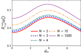
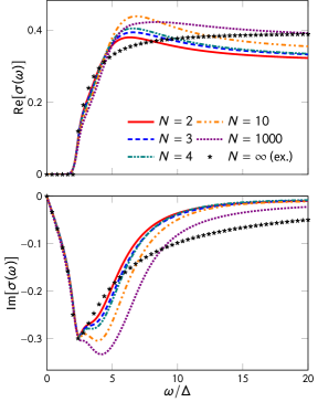
Figure 1: Fixed-point function $\tilde{X}^{*\rm cr}_{1}({\tilde{\omega}_{n}}^{2})$ at the QCP for various values of $N$.

Figure 2: Real and imaginary parts of the conductivity $\sigma(\omega)$ in the disordered phase for various values of $N$. Black stars show the exact large-$N$ solution.

Table 1: Universal conductivity $\sigma^{*}/\sigma_{Q}$ at the QCP,not obtained with a regulator parameter value of $\alpha=2.25$, compared to results obtained from quantum Monte Carlo simulationsWitczak-Krempa et al. (2014); Chen et al. (2014); Gazit et al. (2013); Katz et al. (2014); Gazit et al. (2014) (QMC) and conformal bootstrapKos et al. (2015) (CB). The exact value for $N\to\infty$ is $\pi/8\simeq 0.3927$.

$N$	NPRG	QMC	CB
2	0.3218	0.355-0.361	0.3554(6)
3	0.3285
4	0.3350
10	0.3599
1000	0.3927

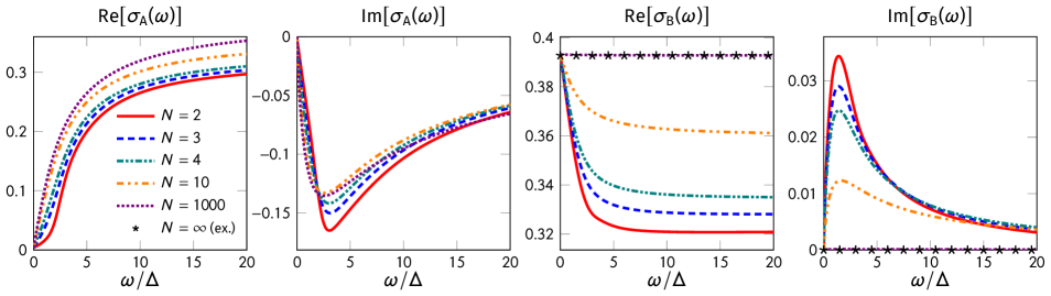
Figure 3: Real and imaginary parts of the conductivity in the ordered phase for various values of $N$. Left: $\sigma_{\rm A}(\omega)$ with the superfluid contribution subtracted. Right: $\sigma_{\rm B}(\omega)$. Black stars show the exact large-$N$ solution $\sigma_{\rm B}(\omega)=\pi/8$.

Conductivity. At the QCP we expect $\sigma(\omega\to 0)/\sigma_{Q}$ to take a nonzero universal value $\sigma^{*}/\sigma_{Q}$.Fisher et al. (1990); not The $k$-dependent conductivity $\sigma_{k}(i\omega_{n})$, as a function of the Matsubara frequency $\omega_{n}$, is given by

$$\sigma_{k}(i\omega_{n})=2\pi\sigma_{Q}\omega_{n}X_{1,k}(\omega_{n}^{2})=2\pi\sigma_{Q}{\tilde{\omega}_{n}}\tilde{X}_{1,k}({\tilde{\omega}_{n}}^{2})$$ (13)

when the order parameter vanishes ($\rho_{0,k}=0$). Here ${\tilde{\omega}_{n}}=\omega_{n}/k$ is a dimensionless frequency and $\tilde{X}_{1,k}({\tilde{\omega}_{n}}^{2})=kX_{1,k}(\omega_{n}^{2})$ a dimensionless function of ${\tilde{\omega}_{n}}^{2}$. At the QCP, the function $\tilde{X}_{1,k}$ reaches a $k$-independent fixed-point value $\tilde{X}^{*\rm cr}_{1}$ and the conductivity takes the form $\sigma_{k}(i\omega_{n})=2\pi\sigma_{Q}{\tilde{\omega}_{n}}\tilde{X}^{*\rm cr}_{1}({\tilde{\omega}_{n}}^{2})$. The low-frequency universal conductivity is obtained by taking first the limit $k\to 0$ and then $\omega_{n}\to 0$, i.e. ${\tilde{\omega}_{n}}\to\infty$: $\sigma^{*}/2\pi\sigma_{Q}=\lim_{{\tilde{\omega}_{n}}\to\infty}{\tilde{\omega}_{n}}\tilde{X}^{*\rm cr}_{1}({\tilde{\omega}_{n}}^{2})$ is thus determined by the $1/{\tilde{\omega}_{n}}$ behavior of $\tilde{X}^{*\rm cr}_{1}({\tilde{\omega}_{n}}^{2})$ at high frequencies (Fig. 2). Note that this $1/{\tilde{\omega}_{n}}$ high-frequency tail, which corresponds to a $1/\omega_{n}$ divergence of $X_{1,k=0}(\omega_{n}^{2})$ for $\omega_{n}\to 0$, is responsible for the breakdown of the derivative expansion of $\Gamma_{k}$ used in Ref. Rose and Dupuis, 2017. The value of $\sigma^{*}$ depends weakly on the regulator, through the arbitrary parameter $\alpha$. This dependence on $\alpha$ decreases as $N$ increases, and at $N=\infty$ the results do not depend on $\alpha$ and the exact value $\sigma^{*}/\sigma_{Q}=\pi/8$ is recovered.Sachdev (2011) The universal conductivity $\sigma^{*}$ is shown in Table 1 for various values of $N$. For $N=2$ we find a value in reasonable agreement with (although 10% smaller than) results from QMCWitczak-Krempa et al. (2014); Chen et al. (2014); Gazit et al. (2013); Katz et al. (2014); Gazit et al. (2014) and conformal bootstrap.Kos et al. (2015)

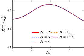
Figure 4: Fixed-point function $\tilde{X}^{*\rm ord}_{1}({\tilde{\omega}_{n}}^{2})$ in the ordered phase for various values of $N$. The universal conductivity $\sigma_{\rm B}^{*}$ is determined by the $1/{\tilde{\omega}_{n}}$ high-frequency tail and the collapse of the curves indicates that $\sigma_{\rm B}^{*}$ is $N$-independent.

In the disordered phase, away from the QCP, Eq. (13) still holds since the order parameter vanishes. In Fig. 2 we show the real-frequency conductivity $\sigma(\omega)$ obtained from $\sigma_{k=0}(i\omega_{n})$ by analytical continuation using Padé approximants,Vidberg and Serene (1977) a method which has proven to be reliable in the NPRG approach.Rose et al. (2015, 2016); Rose and Dupuis (2017) As expected, the system is insulating. The real part of the conductivity vanishes below the two-particle excitation gap $2\Delta$ and the system behaves as a perfect capacitor for $|\omega|\ll\Delta$, i.e. $\sigma(\omega)\simeq-iC_{\rm dis}\omega$, with capacitance (per unit area) $C_{\rm dis}=2\pi\hbar\sigma_{Q}X_{1,k=0}(\omega_{n}^{2}=0)$. Note that for large-$N$, there is a discrepancy between the exact solution and our computation. Indeed, unlike at the QCP and in the ordered phase, in the disordered phase the LPA^′′ does not reproduce the large $N$ solution. Furthermore, the analytic continuation is made difficult by the singularity at $\omega=2\Delta$ so that the frequency dependence of $\sigma(\omega)$ above $2\Delta$ should be taken with caution.

Let us finally discuss the two elements, $\sigma_{\rm A}$ and $\sigma_{\rm B}$, of the conductivity tensor in the ordered phase where the O($N$) symmetry is spontaneously broken:

$$\begin{split}\sigma_{{\rm A},k}(i\omega_{n})={}&2\pi\sigma_{Q}\{\omega_{n}X_{1,k}(\omega_{n}^{2})+(2\rho_{0,k}/\hbar)\\ &\times[Z_{k}(\omega_{n}^{2})/\omega_{n}+\omega_{n}X_{2,k}(\omega_{n}^{2})]\},\\ \sigma_{{\rm B},k}(i\omega_{n})={}&2\pi\sigma_{Q}\omega_{n}X_{1,k}(\omega_{n}^{2}).\end{split}$$ (14)

At low frequencies, $\sigma_{{\rm A},k}(i\omega_{n})/2\pi\sigma_{Q}\simeq 2\rho_{0,k}Z_{k}(0)/\hbar\omega_{n}$ is characteristic of a superfluid system with stiffness $\rho_{s,k}=2\rho_{0,k}Z_{k}(0)$ (i.e. a perfect inductor with inductance $L_{\rm ord}=\hbar/2\pi\sigma_{Q}\rho_{s}$). $\sigma_{\rm A}(\omega)$, with the superfluid contribution subtracted, is shown in Fig. 3. Our results seem to indicate the absence of a constant ${\cal O}(\omega_{n}^{0})$ term in agreement with the predictions of perturbation theory.Podolsky et al. (2011) Furthermore we see a marked difference in the low-frequency behavior of the real part of the conductivity between the cases $N=2$ and $N\neq 2$, but our numerical results are not precise enough to resolve the low-frequency power laws (predictedPodolsky et al. (2011) to be $\omega$ and $\omega^{5}$ for $N\neq 2$ and $N=2$, respectively). On the other hand we find that $\sigma_{\rm B}(\omega)$ reaches a nonzero universal value $\sigma_{\rm B}^{*}$ in the limit $\omega\to 0$ (Fig. 3). As for the conductivity at the QCP, this universal value is determined by the $1/{\tilde{\omega}_{n}}$ high-frequency tail of the fixed-point value $\tilde{X}_{1}^{*\rm ord}({\tilde{\omega}_{n}}^{2})$ of the dimensionless function $\tilde{X}_{1,k}({\tilde{\omega}_{n}}^{2})$. Quite surprisingly, and contrary to $\tilde{X}_{1}^{*\rm cr}$ (Fig. 2), $\tilde{X}_{1}^{*\rm ord}$ turns out to be $N$ independent: the relative change in $\tilde{X}_{1}^{*\rm ord}$ is less than $10^{-6}$ when $N$ varies (Fig. 4). Noting that the obtained value $\sigma_{\rm B}^{*}/\sigma_{Q}\simeq 0.3927$ is equal to the large-$N$ resultRose and Dupuis (2017); Lucas et al. (2017) $\pi/8$ within numerical precision, we conjecture that $\sigma_{\rm B}^{*}/\sigma_{Q}=\pi/8$ for all values of $N$.

This result can be simply understood by noting that Goldstone bosons become effectively noninteracting in the infrared limit. Using the renormalized Goldstone-boson propagator $G_{\rm T}({\bf p},i\omega_{n})=[Z({\bf p}^{2}+\omega_{n}^{2})]^{-1}$, where $Z=\rho_{s}/2\rho_{0}$ is the field renormalization factor, and noting $Z_{B}$ the renormalization factor associated with the boson–gauge-field interaction for a class B generator, an elementary calculation then gives $\sigma_{\rm B}^{*}/\sigma_{Q}=(Z_{B}/Z)^{2}\pi/8$. Gauge invariance implies that $Z_{B}$ and $Z$ are not independent but related by the Ward identity $Z_{B}=Z$, so that we finally obtain $\sigma_{\rm B}^{*}/\sigma_{Q}=\pi/8$ in agreement with the NPRG result.

Conclusion. We have determined the frequency-dependent zero-temperature conductivity near a relativistic $(2+1)$-dimensional QCP with an O($N$)-symmetric order parameter. Our results are obtained using the LPA^′′, an approximation of the exact RG flow equation satisfied by the effective action which respects the local gauge invariance of the theory while retaining the full momentum/frequency dependence of the vertices. Besides the frequency dependence of the conductivity both in the ordered and disordered phases, our main result is the conjecture that $\sigma_{\rm B}(\omega\to 0)/\sigma_{Q}$ takes the superuniversal ($N$-independent) value $\sigma_{\rm B}^{*}/\sigma_{Q}=\pi/8$.not This result could in principle be confirmed experimentally in two-dimensional quantum antiferromagnets, where both quantum criticality and the Higgs amplitude mode have been recently observed,Jain et al. (2017); Souliou et al. (2017) although the frequency-dependent spin conductivity has not been measured so far. A natural continuation of this work would be to extend the NPRG procedure to finite temperatures to investigate both the collisionless ($\omega\gg T$) and hydrodynamic ($\omega\ll T$) regimes, the latter being inaccesible at zero temperature.

Acknowledgment We thank N. Defenu for pointing out Refs. Casetti et al., 2011; Nerattini et al., 2014 and P. Kopietz for correspondence.

References

- Sachdev (2011) S. Sachdev, Quantum Phase Transitions, 2nd ed. (Cambridge University Press, Cambridge, England, 2011).
- Fisher et al. (1990) Matthew P. A. Fisher, G. Grinstein, and S. M. Girvin, “Presence of quantum diffusion in two dimensions: Universal resistance at the superconductor-insulator transition,” Phys. Rev. Lett. 64, 587–590 (1990).
- (3) We consider only zero-temperature coherent transport where the DC conductivity is defined by the limit and or, equivalently, with .
- Witczak-Krempa et al. (2014) William Witczak-Krempa, Erik S. Sørensen, and Subir Sachdev, “The dynamics of quantum criticality revealed by quantum Monte Carlo and holography,” Nature Physics 10, 361 (2014).
- Chen et al. (2014) Kun Chen, Longxiang Liu, Youjin Deng, Lode Pollet, and Nikolay Prokof’ev, “Universal Conductivity in a Two-Dimensional Superfluid-to-Insulator Quantum Critical System,” Phys. Rev. Lett. 112, 030402 (2014).
- Gazit et al. (2013) Snir Gazit, Daniel Podolsky, Assa Auerbach, and Daniel P. Arovas, “Dynamics and conductivity near quantum criticality,” Phys. Rev. B 88, 235108 (2013).
- Katz et al. (2014) Emanuel Katz, Subir Sachdev, Erik S. Sørensen, and William Witczak-Krempa, “Conformal field theories at nonzero temperature: Operator product expansions, monte carlo, and holography,” Phys. Rev. B 90, 245109 (2014).
- Gazit et al. (2014) Snir Gazit, Daniel Podolsky, and Assa Auerbach, “Critical Capacitance and Charge-Vortex Duality Near the Superfluid-to-Insulator Transition,” Phys. Rev. Lett. 113, 240601 (2014).
- Kos et al. (2015) Filip Kos, David Poland, David Simmons-Duffin, and Alessandro Vichi, “Bootstrapping the O() archipelago,” J. High Energy Phys. 2015, 106 (2015).
- Rose and Dupuis (2017) F. Rose and N. Dupuis, “Nonperturbative functional renormalization-group approach to transport in the vicinity of a -dimensional O()-symmetric quantum critical point,” Phys. Rev. B 95, 014513 (2017).
- Campa et al. (2003) Alessandro Campa, Andrea Giansanti, and Daniele Moroni, “Canonical solution of classical magnetic models with long-range couplings,” J. Phys. A: Math. Gen. 36, 6897 (2003).
- Casetti et al. (2011) Lapo Casetti, Cesare Nardini, and Rachele Nerattini, “Microcanonical Relation between Continuous and Discrete Spin Models,” Phys. Rev. Lett. 106, 057208 (2011).
- Nerattini et al. (2014) Rachele Nerattini, Andrea Trombettoni, and Lapo Casetti, “Critical energy density of O models in ,” J. Stat. Mech. 2014, P12001 (2014).
- Note (1) At zero temperature, the bosonic Matsubara frequency ( integer) becomes a continuous variable.
- Rückriegel and Kopietz (2017) Andreas Rückriegel and Peter Kopietz, “Spin currents, spin torques, and the concept of spin superfluidity,” Phys. Rev. B 95, 104436 (2017).
- Damle and Sachdev (1997) Kedar Damle and Subir Sachdev, “Nonzero-temperature transport near quantum critical points,” Phys. Rev. B 56, 8714–8733 (1997).
- Berges et al. (2002) J. Berges, N. Tetradis, and C. Wetterich, “Non-perturbative renormalization flow in quantum field theory and statistical physics,” Phys. Rep. 363, 223 (2002).
- Delamotte (2012) Bertrand Delamotte, “An Introduction to the Nonperturbative Renormalization Group,” in Renormalization Group and Effective Field Theory Approaches to Many-Body Systems, Lecture Notes in Physics, Vol. 852, edited by A. Schwenk and J. Polonyi (Springer Berlin Heidelberg, 2012) pp. 49–132.
- Kopietz et al. (2010) P. Kopietz, L. Bartosch, and F. Schütz, Introduction to the Functional Renormalization Group (Springer, Berlin, 2010).
- Wetterich (1993) C. Wetterich, “Exact evolution equation for the effective potential,” Phys. Lett. B 301, 90 (1993).
- Hasselmann (2012) N. Hasselmann, “Effective-average-action-based approach to correlation functions at finite momenta,” Phys. Rev. E 86, 041118 (2012).
- Canet et al. (2010) For applications of the LPA′′ in different contexts (KPZ equation and turbulence), see Léonie Canet, Hugues Chaté, Bertrand Delamotte, and Nicolás Wschebor, “Nonperturbative Renormalization Group for the Kardar-Parisi-Zhang Equation,” Phys. Rev. Lett. 104, 150601 (2010).
- Canet et al. (2011) Léonie Canet, Hugues Chaté, Bertrand Delamotte, and Nicolás Wschebor, “Nonperturbative renormalization group for the Kardar-Parisi-Zhang equation: General framework and first applications,” Phys. Rev. E 84, 061128 (2011).
- Canet et al. (2012) Léonie Canet, Hugues Chaté, Bertrand Delamotte, and Nicolás Wschebor, “Erratum: Nonperturbative renormalization group for the Kardar-Parisi-Zhang equation: General framework and first applications [Phys. Rev. E 84, 061128 (2011)],” Phys. Rev. E 86, 019904(E) (2012).
- Canet et al. (2016) Léonie Canet, Bertrand Delamotte, and Nicolás Wschebor, “Fully developed isotropic turbulence: Nonperturbative renormalization group formalism and fixed-point solution,” Phys. Rev. E 93, 063101 (2016).
- Note (2) There is no optimal value of which extremizes the value of the conductivity, i.e. such that . However varies at most only by a few percents when varies in the range . We retain , which yields the best estimates for the critical exponents.
- Vidberg and Serene (1977) H. J. Vidberg and J. W. Serene, “Solving the Eliashberg equations by means of N-point Padé approximants,” J. Low Temp. Phys. 29, 179–192 (1977).
- Rose et al. (2015) F. Rose, F. Léonard, and N. Dupuis, “Higgs amplitude mode in the vicinity of a -dimensional quantum critical point: A nonperturbative renormalization-group approach,” Phys. Rev. B 91, 224501 (2015).
- Rose et al. (2016) F. Rose, F. Benitez, F. Léonard, and B. Delamotte, “Bound states of the model via the nonperturbative renormalization group,” Phys. Rev. D 93, 125018 (2016).
- Note (3) This is due to the fact that the full dependence of the functions , , and is not taken into account.
- Podolsky et al. (2011) Daniel Podolsky, Assa Auerbach, and Daniel P. Arovas, “Visibility of the amplitude (Higgs) mode in condensed matter,” Phys. Rev. B 84, 174522 (2011).
- Lucas et al. (2017) Andrew Lucas, Snir Gazit, Daniel Podolsky, and William Witczak-Krempa, “Dynamical Response near Quantum Critical Points,” Phys. Rev. Lett. 118, 056601 (2017).
- Note (4) The infrared asymptotic freedom of the Goldstone bosons is explicit in the nonlinear sigma model description where the coupling constant vanishes in the low-energy limit in the ordered phase.
- Note (5) A similar Ward identify exists in Fermi-liquid theory, ensuring that the quasi-particle weight does not appear in physical response functions.
- Jain et al. (2017) A. Jain, M. Krautloher, J. Porras, G. H. Ryu, D. P. Chen, D. L. Abernathy, J. T. Park, A. Ivanov, J. Chaloupka, G. Khaliullin, B. Keimer, and B. J. Kim, “Higgs mode and its decay in a two-dimensional antiferromagnet,” Nature Phys. 13, 633 (2017).
- Souliou et al. (2017) Sofia-Michaela Souliou, Jivrí Chaloupka, Giniyat Khaliullin, Gihun Ryu, Anil Jain, B. J. Kim, Matthieu Le Tacon, and Bernhard Keimer, “Raman Scattering from Higgs Mode Oscillations in the Two-Dimensional Antiferromagnet ,” Phys. Rev. Lett. 119, 067201 (2017).