A comparison of Euclidean and Heisenberg Hausdorff measures

Abstract

We prove some geometric properties of sets in the first Heisenberg group whose Heisenberg Hausdorff dimension is the minimal or maximal possible in relation to their Euclidean one and the corresponding Hausdorff measures are positive and finite. In the first case we show that these sets must be in a sense horizontal and in the second case vertical. We show the sharpness of our results with some examples.

1 Introduction

Let $\mathcal{H}^{s}_{E}$ denote the Euclidean Hausdorff measure in the first Heisenberg group $\mathbb{H}^{1}$ and let $\mathcal{H}^{s}_{H}$ denote the Hausdorff measure with respect to some homogeneous metric. Let $\dim_{E}$ and $\dim_{H}$ denote the corresponding Hausdorff dimensions. Generally, for a set $A\subset\mathbb{H}^{1}$, $\dim_{E}A$ and $\dim_{H}A$ can be different. Balogh, Rickly and Serra Cassano in [BRSC] compared them, proving what follows. For $s\geq 0$ let

$$\beta_{-}(s)=\max\{s,2s-2\},\beta_{+}(s)=\min\{2s,s+1\}.$$

Then for any $A\subset\mathbb{H}^{1}$,

$$\beta_{-}(\dim_{E}A)\leq\dim_{H}A\leq\beta_{+}(\dim_{E}A).$$

Moreover, they also showed the sharpness of some of these inequalities, which was then completed by Balogh and Tyson in [BT]: for any $0<s<3$ they constructed compact subsets $F_{1}$ and $F_{2}$ of $\mathbb{H}^{1}$ such that $\mathcal{H}^{s}_{E}(F_{1})$ and $\mathcal{H}^{\beta_{-}(s)}_{H}(F_{1})$ are positive and finite and $\mathcal{H}^{s}_{E}(F_{2})$ and $\mathcal{H}^{\beta_{+}(s)}_{H}(F_{2})$ are positive and finite. The example $F_{1}$, for $0<s\leq 2$, is in a sense horizontal and $F_{2}$ is in a sense vertical. In this paper we show that this must be so. We prove in Theorem 2 that for any set $A\subset\mathbb{H}^{1}$ and $0<s\leq 2$, if both $\mathcal{H}^{s}_{E}(A)$ and $\mathcal{H}^{s}_{H}(A)$ are positive and finite, then in some arbitrarily small neighbourhoods around its typical points $p$, most of $A$ lies close to the horizontal plane through $p$. We shall construct an example (see Example 5) to show that this need not hold for all small neighbourhoods and another example (see Example 7) to show that this does not hold when $s>2$ and both $\mathcal{H}^{s}_{E}(A)$ and $\mathcal{H}^{2s-2}_{H}(A)$ are positive and finite. Corresponding to the second case we show in Theorems 3 and 4 that if both $\mathcal{H}^{s}_{E}(A)$ and $\mathcal{H}^{\beta_{+}(s)}_{H}(A)$ are positive and finite, then in some arbitrarily small neighbourhoods around its typical points $p$, a large part of $A$ lies off the horizontal plane through $p$.

In [BTW] Balogh, Tyson and Warhurst solved the dimension comparison problem in general Carnot groups, but here we restrict to the first Heisenberg group.

2 Preliminaries

In a metric space $X$ for $0<s<\infty$ the $s$-dimensional Hausdorff measure of $A\subset X$ is defined by

$$\mathcal{H}^{s}(A)=\lim_{\delta\to 0}\mathcal{H}^{s}_{\delta}(A),$$

where

$$\mathcal{H}^{s}_{\delta}(A)=\inf\{\sum_{i=1}^{\infty}\operatorname{diam}(B_{i})^{s}:A\subset\bigcup_{i=1}^{\infty}B_{i},\operatorname{diam}(B_{i})<\delta\}.$$

The Hausdorff dimension of $A$ is

$$\dim A=\inf\{s:\mathcal{H}^{s}(A)=0\}.$$

Let $B(p,r)$ be the closed ball with centre $p\in X$ and radius $r$. We have the basic upper density theorem for Hausdorff measures, see, e,g., [F], 2.10.19.

Theorem 1.

Let $A\subset X$ be $\mathcal{H}^{s}$ measurable with $\mathcal{H}^{s}(A)<\infty$. Then for $\mathcal{H}^{s}$ almost all $p\in A$,

$$2^{-s}\leq\limsup_{r\to 0}\frac{\mathcal{H}^{s}(A\cap B(p,r))}{(2r)^{s}}\leq 1$$

and for $\mathcal{H}^{s}$ almost all $p\in X\setminus A$,

$$\lim_{r\to 0}\frac{\mathcal{H}^{s}(A\cap B(p,r))}{(2r)^{s}}=0.$$

Let $\mathbb{H}^{1}$ be the first Heisenberg group. It can be identified as $\mathbb{R}^{3}$ with the non-Abelian group operation

$$p\cdot p^{\prime}=(x+x^{\prime},y+y^{\prime},t+t^{\prime}+2(x^{\prime}y-xy^{\prime})),$$

for $p=(x,y,t),p^{\prime}=(x^{\prime},y^{\prime},t^{\prime})$, and with the metric

$$d_{H}(p,p^{\prime})=\left(((x-x^{\prime})^{2}+(y-y^{\prime})^{2})^{2}+(t-t^{\prime}-2(x^{\prime}y-xy^{\prime}))^{2}\right)^{1/4}.$$

In addition to $d_{H}$ we shall also use the Euclidean metric, which we denote by $d_{E}$. Then for $0<R<\infty$ there exists a constant $c_{R}>0$ such that for every $p,p^{\prime}\in B_{E}(0,R)$,

$$\frac{1}{c_{R}}d_{E}(p,p^{\prime})\leq d_{H}(p,p^{\prime})\leq c_{R}d_{E}(p,p^{\prime})^{1/2}.$$ (1)

The closed ball $B(p,r)$ is denoted by $B_{H}(p,r)$ when the metric is $d_{H}$ and by $B_{E}(p,r)$ when the metric is $d_{E}$. The $s$-dimensional Hausdorff measures and dimensions with respect to $d_{H}$ and $d_{E}$ are denoted by $\mathcal{H}_{H}^{s},\mathcal{H}_{E}^{s},\dim_{H}$ and $\dim_{E}$. In place of $d_{H}$ we could use any homogeneous metric on $\mathbb{H}^{1}$, that is, any left invariant metric $d$ satisfying $d((\delta x,\delta y,\delta^{2}t),(\delta x^{\prime},\delta y^{\prime},\delta^{2}t^{\prime}))=\delta d((x,y,t),(x^{\prime},y^{\prime},t^{\prime}))$. By [BLU], 5.1.5, they are all equivalent.

Recall the definitions of $\beta_{-}(s)$ and $\beta_{+}(s)$ from the introduction. Then by [BTW], Proposition 3.1, for any positive number $R$ there exists a constant $C_{R}$ such that for $A\subset B_{E}(0,R)$ and for $0<s<3$,

$$\mathcal{H}^{\beta_{+}(s)}_{H}(A)/C_{R}\leq\mathcal{H}^{s}_{E}(A)\leq C_{R}\mathcal{H}^{\beta_{-}(s)}_{H}(A).$$ (2)

Let $V(p)$ denote the horizontal plane passing through $p=(x_{0},y_{0},t_{0})\in\mathbb{H}^{1}$. This is the set of points $q=(x,y,t)$ such that

$$t_{0}-t-2(xy_{0}-yx_{0})=0.$$ (3)

The Euclidean distance of a point $q=(x,y,t)$ to the plane $V(p)$ is

$$d_{E}(q,V(p))=\frac{|t_{0}-t-2(xy_{0}-yx_{0})|}{\sqrt{1+4(x_{0}^{2}+y_{0}^{2})}}.$$ (4)

We let $A(\delta)$ denote the closed $\delta$ neighbourhood of $A\subset\mathbb{H}^{1}$ in the Euclidean metric. Observe that $B_{H}(p,r)$ looks like $V(p)(r^{2})\cap B_{E}(p,r)$, more precisely, for $p$ as above with $x_{0}^{2}+y_{0}^{2}\leq R^{2}$,

$$V(p)\left(\frac{r^{2}}{\sqrt{2(1+4R^{2})}}\right)\cap B_{E}\left(p,\frac{r}{2}\right)\subset B_{H}(p,r)\subset V(p)(r^{2})\cap B_{E}(p,r).$$ (5)

The restriction of a measure $\mu$ to a set $A\subset X$ is denoted by $\mu\mathbin{\vrule height=6.88889pt,depth=0.0pt,width=0.55974pt\vrule height=0.55974pt,depth=0.0pt,width=5.59721pt}A;\mu\mathbin{\vrule height=6.88889pt,depth=0.0pt,width=0.55974pt\vrule height=0.55974pt,depth=0.0pt,width=5.59721pt}A(B)=\mu(A\cap B)$.

3 The theorems

Theorem 2.

Let $0<s\leq 2$ and let $A\subset\mathbb{H}^{1}$ be such that $\mathcal{H}^{s}_{H}(A)<\infty$. Then for $\mathcal{H}^{s}_{E}$ almost every $p\in A$ there exists $0<\epsilon<1$ such that

$$\liminf_{r\rightarrow 0}\frac{\mathcal{H}^{s}_{E}(A\cap B_{E}(p,r)\setminus V(p)(r^{1+\epsilon}))}{r^{s}}=0.$$

Proof.

By the Borel regularity of Hausdorff measures we may assume that $A$ is a Borel set. Changing $\epsilon$ a bit it suffices to prove for $\mathcal{H}^{s}_{E}$ almost every $p\in A$ that

$$\liminf_{r\rightarrow 0}\frac{\mathcal{H}^{s}_{E}(A\cap B_{E}(p,r)\setminus V(p)(7r^{1+\epsilon}))}{r^{s}}=0.$$ (6)

We may assume that for some positive number $R$,

$$A\subset B_{E}(0,R).$$

First, let us see that we can reduce to the case when there is a positive number $C$ such that

$$\frac{1}{C}\mathcal{H}^{s}_{E}(B)\leq\mathcal{H}^{s}_{H}(B)\leq C\mathcal{H}^{s}_{E}(B)$$ (7)

for every $B\subset A$. The left-hand side inequality holds because of (1). We can decompose $A$ as

$$A=C\cup D,$$

where

$$\mathcal{H}^{s}_{E}(C)=0\quad\mbox{and}\quad\mathcal{H}^{s}_{E}(B)=0\Leftrightarrow\mathcal{H}^{s}_{H}(B)=0\quad\forall B\subset D.$$ (8)

This can be done as follows. Let $\mu_{E}=\mathcal{H}^{s}_{E}\mathbin{\vrule height=6.88889pt,depth=0.0pt,width=0.55974pt\vrule height=0.55974pt,depth=0.0pt,width=5.59721pt}{A}$ and $\mu_{H}=\mathcal{H}^{s}_{H}\mathbin{\vrule height=6.88889pt,depth=0.0pt,width=0.55974pt\vrule height=0.55974pt,depth=0.0pt,width=5.59721pt}A$. Since $\mu_{E}<<\mu_{H}$, we have that for every Borel set $B\subset\mathbb{H}^{1}$,

$$\mu_{E}(B)=\int_{B}D(\mu_{E},\mu_{H},x)d\mu_{H}x,$$

where $D(\mu_{E},\mu_{H},x)$ is the Radon-Nikodym derivative of $\mu_{E}$ with respect to $\mu_{H}$. Thus if we let

$$C=\{x\in A:D(\mu_{E},\mu_{H},x)=0\},\quad D=\{x\in A:D(\mu_{E},\mu_{H},x)>0\},$$

then $C$ and $D$ satisfy (8). Moreover, we can write

$$D=\bigcup_{j=1}^{\infty}D_{j},\quad\mbox{where}\quad\mathcal{H}^{s}_{E}(B)\geq\frac{1}{j}\mathcal{H}^{s}_{H}(B)\quad\forall B\subset D_{j}$$

by taking

$$D_{j}=\{x\in D:D(\mu_{E},\mu_{H},x)>\frac{1}{j}\}.$$

Thus (7) holds for every $D_{j}$ in place of $A$. If we can prove (6) under the assumption (7), and so for every $D_{j}$, it follows that (6) holds for $A$ by the the second part of the upper density theorem 1. Hence we can assume (7).

Let $\epsilon>0$. Suppose that (6) is false. Then by Theorem 1 there exist $c>0$, $0<r_{0}<1$ and $A^{\prime}\subset A$, $\mathcal{H}^{s}_{E}(A^{\prime})>0$, such that

$$\mathcal{H}^{s}_{E}(A\cap B_{E}(p,r))\leq 3^{s}r^{s}$$ (9)

and

$$\mathcal{H}^{s}_{E}(A\cap B_{E}(p,r)\setminus V(p)(7r^{1+\epsilon}))>cr^{s}$$ (10)

for every $p\in A^{\prime}$ and $0<r<r_{0}$. Let $0<r<r_{0}/5$ and $p\in A^{\prime}$ be such that $r^{2}<<r^{1+\epsilon}$ and

$$\mathcal{H}^{s}_{E}(B_{H}(p,r)\cap A^{\prime})\geq\frac{1}{C}\mathcal{H}^{s}_{H}(B_{H}(p,r)\cap A^{\prime})>c^{\prime}r^{s}$$ (11)

with $c^{\prime}=1/(2C)$ (we can find these by Theorem 1). Let $k\in\mathbb{N}$ be such that $r^{2}<r^{(1+\epsilon)^{k}}$ and $r^{2}\geq r^{(1+\epsilon)^{k+1}}$, whence $k\geq\log 2/(2\log(1+\epsilon))$. By the $5r$ covering theorem, see, e.g., Theorem 2.1 in [M], for $j=1,\dots,k$ we can find $p_{j,i}\in A^{\prime}\cap B_{H}(p,r)$ such that

$$A^{\prime}\cap B_{H}(p,r)=\bigcup_{i=1}^{m_{j}}A^{\prime}\cap B_{H}(p,r)\cap B_{E}(p_{j,i},5r^{(1+\epsilon)^{j}}),$$ (12)

where the balls $B_{E}(p_{j,i},r^{(1+\epsilon)^{j}})$, $i=1,\dots,m_{j}$, are disjoint. Since by (11), (12) and (9),

$$c^{\prime}r^{s} <\mathcal{H}^{s}_{E}(B_{H}(p,r)\cap A^{\prime})$$

$$\leq\sum_{i=1}^{m_{j}}\mathcal{H}^{s}_{E}(A^{\prime}\cap B_{H}(p,r)\cap B_{E}(p_{j,i},5r^{(1+\epsilon)^{j}}))$$

$$\leq m_{j}3^{s}5^{s}r^{s(1+\epsilon)^{j}},$$

we obtain

$$m_{j}\geq c_{1}r^{s(1-(1+\epsilon)^{j})},$$ (13)

with $c_{1}=c^{\prime}/15^{s}$ depending only on $s$ and $C$.

We can show that the sets

$$\bigcup_{i=1}^{m_{j}}B_{E}(p_{j,i},r^{(1+\epsilon)^{j}})\setminus V(p_{j,i})(7r^{(1+\epsilon)^{j+1}}),\ j=1,\dots,k,$$ (14)

are disjoint. Let $j\in\{1,\dots,k-1\}$ and let $B_{E}(p_{j,i},r^{(1+\epsilon)^{j}})$ and $B_{E}(p_{n,l},r^{(1+\epsilon)^{n}})$, $j+1\leq n\leq k$, $i\in\{1,\dots,m_{j}\},l\in\{1,\dots,m_{n}\}$, be such that $B_{E}(p_{j,i},r^{(1+\epsilon)^{j}})\cap B_{E}(p_{n,l},r^{(1+\epsilon)^{n}})\neq\emptyset$. We want to show that

$$(B_{E}(p_{j,i},r^{(1+\epsilon)^{j}})\setminus V(p_{j,i})(7r^{(1+\epsilon)^{j+1}}))\cap B_{E}(p_{n,l},r^{(1+\epsilon)^{n}})=\emptyset.$$ (15)

Let us denote $p=(\bar{x},\bar{y},\bar{t})$, $p_{j,i}=(x_{i},y_{i},t_{i})$, $p_{n,l}=(x_{l},y_{l},t_{l})$. Since $p_{j,i},p_{n,l}\in B_{H}(p,r)$, we have

$$((\bar{x}-x_{i})^{2}+(\bar{y}-y_{i})^{2})^{2}+(\bar{t}-t_{i}-2(x_{i}\bar{y}-y_{i}\bar{x}))^{2}\leq r^{4},$$ (16)

and

$$((\bar{x}-x_{l})^{2}+(\bar{y}-y_{l})^{2})^{2}+(\bar{t}-t_{l}-2(x_{l}\bar{y}-y_{l}\bar{x}))^{2}\leq r^{4}.$$ (17)

Moreover,

$$d_{E}(p_{j,i},p_{n,l})\leq r^{(1+\epsilon)^{j}}+r^{(1+\epsilon)^{n}}\leq 2r^{(1+\epsilon)^{j}}.$$ (18)

We now want to show that $d_{E}(p_{n,l},V(p_{j,i}))\leq 6r^{(1+\epsilon)^{j+1}}$. Indeed by (4), (16), (17) and (18) we have

$$d_{E}(p_{n,l},V(p_{j,i})) =\frac{|t_{i}-t_{l}-2(x_{l}y_{i}-y_{l}x_{i})|}{\sqrt{1+4(y_{i}^{2}+x_{i}^{2})}}$$

$$\leq |t_{i}-t_{l}-2(x_{l}y_{i}-y_{l}x_{i})|$$

$$\leq |\bar{t}-t_{l}-2(x_{l}\bar{y}-y_{l}\bar{x})|+|2(y_{l}\bar{x}-x_{l}\bar{y})+2(x_{i}\bar{y}-y_{i}\bar{x})+2(x_{l}y_{i}-y_{l}x_{i})|$$

$$+|t_{i}-\bar{t}+2(x_{i}\bar{y}-y_{i}\bar{x})|$$

$$\leq 2r^{2}+2|(x_{l}-x_{i})(y_{i}-\bar{y})-(y_{l}-y_{i})(x_{i}-\bar{x})|$$

$$= 2r^{2}+2|\langle(x_{l}-x_{i},y_{i}-y_{l}),(y_{i}-\bar{y},x_{i}-\bar{x})\rangle|$$

$$\leq 2r^{2}+4r^{(1+\epsilon)^{j}}r\leq 6r^{2},$$

where $\langle\cdot,\cdot\rangle$ denotes the scalar product and we used Cauchy-Schwarz inequality. Since $r^{2}<r^{(1+\epsilon)^{k}}\leq r^{(1+\epsilon)^{j+1}}$, we have $d_{E}(p_{n,l},V(p_{j,i}))\leq 6r^{(1+\epsilon)^{j+1}}$. Thus

$$B_{E}(p_{n,l},r^{(1+\epsilon)^{n}})\subset V(p_{j,i})(7r^{(1+\epsilon)^{j+1}}),$$

which implies (15). Hence the sets in (14) are disjoint.

We have $\mathcal{H}^{s}_{E}(A\cap B_{E}(p_{j,i},r^{(1+\epsilon)^{j}})\setminus V(p_{j,i})(7r^{(1+\epsilon)^{j+1}}))>cr^{s(1+\epsilon)^{j}}$ by (10) hence using (13) we get

$$\begin{split}\mathcal{H}^{s}_{E}(A\cap B_{E}(p,3r))&\geq\sum_{j=1}^{k}\sum_{i=1}^{m_{j}}\mathcal{H}^{s}_{E}(A\cap B_{E}(p_{j,i},r^{(1+\epsilon)^{j}})\setminus V(p_{j,i})(7r^{(1+\epsilon)^{j+1}}))\\ &\geq c\sum_{j=1}^{k}m_{j}r^{s(1+\epsilon)^{j}}\geq cc_{1}\sum_{j=1}^{k}r^{s(1-(1+\epsilon)^{j})}r^{s(1+\epsilon)^{j}}\\ &=cc_{1}kr^{s}\geq cc_{1}\log 2/(2\log(1+\epsilon))r^{s}.\end{split}$$

When $\epsilon$ is small enough, the last term is greater than $7^{s}r^{s}$. This yields a contradiction with Theorem 1. ∎

Remark.

The above proof shows that if $A\subset B_{E}(0,R)$ satisfies (7), then we can choose $\epsilon$ depending only on $s,R$ and $C$.

Theorem 3.

Let $s\geq 1$ and $A\subset\mathbb{H}^{1}$ be such that $\mathcal{H}^{s}_{E}(A)<\infty$. Then for $\mathcal{H}^{s+1}_{H}$ almost every $p\in A$ there exists $\delta>0$ such that

$$\limsup_{r\rightarrow 0}\frac{\mathcal{H}^{s}_{E}(A\cap B_{E}(p,r)\setminus V(p)(\delta r))}{(2r)^{s}}>\frac{1}{2^{s+1}}.$$ (19)

Proof.

We may assume that $A$ is a Borel set and $A\subset B_{E}(0,R)$ for some $R>0$. We can again reduce to the case where there exists a constant $C>0$ such that for every $B\subset A$ we have

$$\frac{1}{C}\mathcal{H}^{s}_{E}(B)\leq\mathcal{H}^{s+1}_{H}(B)\leq C\mathcal{H}^{s}_{E}(B).$$ (20)

Indeed, this follows from a similar reasoning as was used to prove the right-hand side inequality in (7) since $\mathcal{H}^{s+1}_{H}<<\mathcal{H}^{s}_{E}$ holds always by (2) (when $s\geq 1$, $\beta_{+}(s)=s+1$).

By Theorem 1 for $\mathcal{H}^{s}_{E}$ almost all $p\in A$ there exists $0<r_{p}<1$ such that for every $0<r<r_{p}$

$$\mathcal{H}^{s}_{E}(A\cap B_{E}(p,r))\leq 3^{s}r^{s}$$ (21)

and

$$\mathcal{H}^{s+1}_{H}(A\cap B_{H}(p,r))\leq 3^{s+1}r^{s+1}.$$ (22)

For $j=1,2,\dots$, let

$$A_{j}=\{p\in A:2^{-j}\leq r_{p}<2^{-j+1}\}.$$

Then $\mathcal{H}^{s}_{E}(A\setminus\cup_{j=1}^{\infty}A_{j})=0$.

Let $p\in A_{l}$ and $\mathcal{H}^{s}_{E}(A_{l})>0$ for some $l$ and let

$$0<\delta<\frac{1}{2^{s+2}3^{s+2}C\sqrt{1+4R^{2}}},$$ (23)

where $C$ is as in (20). For every $0<r<2^{-l},r<\delta,$ we want to show that there exist $p_{1},\dots,p_{k}$, $k\approx(\delta/r)\sqrt{1+4R^{2}}$, such that

$$B_{E}(p,r)\cap V(p)(\delta r)\subset\bigcup_{i=1}^{k}B_{H}(p_{i},2r).$$ (24)

Let $p=(\bar{x},\bar{y},\bar{t})$. By (3) the horizontal plane $V(p)$ is the set of points $(x,y,t)\in\mathbb{H}^{1}$ such that

$$\bar{t}-t-2(x\bar{y}-y\bar{x})=0.$$

Let $L(p)$ be the vertical line passing through $p$, that is $L(p)=\{(\bar{x},\bar{y},t):t\in\mathbb{R}\}$. If $q=(\bar{x},\bar{y},t)\in L(p)$ and $d_{E}(q,V(p))\leq\delta r$ then $|t-\bar{t}|\leq\delta r\sqrt{1+4R^{2}}$. Indeed, by (4)

$$\delta r\geq d_{E}(q,V(p))=\frac{|\bar{t}-t-2(\bar{x}\bar{y}-\bar{y}\bar{x})|}{\sqrt{1+4(\bar{x}^{2}+\bar{y}^{2})}}=\frac{|\bar{t}-t|}{\sqrt{1+4(\bar{x}^{2}+\bar{y}^{2})}}\geq\frac{|\bar{t}-t|}{\sqrt{1+4R^{2}}}.$$ (25)

Cover the interval $[\bar{t}-\delta r\sqrt{1+4R^{2}},\bar{t}+\delta r\sqrt{1+4R^{2}}]$ with intervals $[t_{i},t_{i+1}],i=1,\dots,k$, with $t_{i+1}-t_{i}=r^{2}$ and

$$k\leq 3(\delta/r)\sqrt{1+4R^{2}}.$$ (26)

Let

$$p_{i}=(\bar{x},\bar{y},t_{i})\in L(p).$$

If $u\in L(p)\cap V(p)(\delta r)$ then there exists $i$ such that $d_{E}(u,p_{i})\leq r^{2}$ by (25). To see that (24) holds, let $q=(x,y,t)\in B_{E}(p,r)\cap V(p)(\delta r)$ and let $q^{\prime}$ be the point of intersection between the plane passing through $q$ parallel to $V(p)$ and the line $L(p)$. This means that

$$q^{\prime}=(\bar{x},\bar{y},t^{\prime})\quad\mbox{and}\quad t-t^{\prime}-2((\bar{x}-x)\bar{y}-(\bar{y}-y)\bar{x})=0,$$

hence

$$q^{\prime}=(\bar{x},\bar{y},t-2(y\bar{x}-x\bar{y})).$$

Since $q^{\prime}\in L(p)\cap V(p)(\delta r)$, there exists $j\in\{1,\dots,k\}$ such that

$$d_{E}(q^{\prime},p_{j})=|t-2(y\bar{x}-x\bar{y})-t_{j}|\leq r^{2}.$$ (27)

Let us now see that $q\in B_{H}(p_{j},2r)$, that is $d_{H}(q,p_{j})\leq 2r$. Indeed,

$$d_{H}(q,p_{j})^{4}=((x-\bar{x})^{2}+(y-\bar{y})^{2})^{2}+\left(t-t_{j}-2(\bar{x}y-\bar{y}x)\right)^{2}.$$ (28)

Since $q\in B_{E}(p,r)$, we have

$$(x-\bar{x})^{2}+(y-\bar{y})^{2}\leq r^{2},$$

and by (27) the second term in (28) is $\leq r^{4}$. It follows that $d_{H}(q,p_{j})\leq 2r$, which proves (24).

Hence by (24), (20), (22), (26) and (23) we have that for every $0<r<2^{-l},$

$$\mathcal{H}^{s}_{E}(A\cap B_{E}(p,r)\cap V(p)(\delta r)) \leq\sum_{i=1}^{k}\mathcal{H}^{s}_{E}(A\cap B_{H}(p_{i},2r))$$

$$\leq C\sum_{i=1}^{k}\mathcal{H}^{s+1}_{H}(A\cap B_{H}(p_{i},2r))$$

$$\leq Ck3^{s+1}2^{s+1}r^{s+1}$$

$$\leq C3^{s+2}2^{s+1}\frac{\delta}{r}\sqrt{1+4R^{2}}r^{s+1}<\frac{1}{2}r^{s}.$$

Thus for $\mathcal{H}^{s}_{E}$ almost every $p\in A$ there exists $\delta>0$ such that

$$\limsup_{r\rightarrow 0}\frac{\mathcal{H}^{s}_{E}(A\cap B_{E}(p,r)\cap V(p)(\delta r))}{(2r)^{s}}<\frac{1}{2^{s+1}},$$

which proves (19) by Theorem 1. ∎

Remark.

Again, the above proof shows that if $A\subset B_{E}(0,R)$ satisfies (20), then we can choose $\delta$ depending only on $s,R$ and $C$.

Theorem 4.

Let $0<s<1$ and $A\subset\mathbb{H}^{1}$ be such that $\mathcal{H}^{s}_{E}(A)<\infty$. Then for $\mathcal{H}^{2s}_{H}$ almost every $p\in A$ there exists $\delta>0$ such that

$$\limsup_{r\rightarrow 0}\frac{\mathcal{H}^{s}_{E}(A\cap B_{E}(p,r)\setminus V(p)(\delta r))}{(2r)^{s}}>0.$$ (29)

Proof.

We may assume that $A$ is a Borel set and $A\subset B_{E}(0,R)$ for some $R>0$. Since $\mathcal{H}^{2s}_{H}<<\mathcal{H}^{s}_{E}$ always holds (here $\beta_{+}(s)=2s$ because $s<1$), we can assume, as in the proof of Theorem 3, that there exists $C>0$ such that

$$\frac{1}{C}\mathcal{H}^{s}_{E}(B)\leq\mathcal{H}^{2s}_{H}(B)\leq C\mathcal{H}^{s}_{E}(B)$$ (30)

for every $B\subset A$.

Suppose that (29) does not hold. Let $A_{0}\subset A$ be a Borel set such that $\mathcal{H}^{s}_{E}(A_{0})>0$ and that (29) fails for $p\in A_{0}$ for every $\delta>0$. Fix $\delta>0$ and $\epsilon>0$, to be chosen sufficiently small at the end of the proof. Then there exist a Borel set $A^{\prime}\subset A_{0}$ and $r_{0}>0$ such that $\mathcal{H}^{s}_{E}(A^{\prime})>\mathcal{H}^{s}_{E}(A_{0})/2$ and for every $p\in A^{\prime}$ and for every $0<r<r_{0}$,

$$\mathcal{H}^{s}_{E}(A\cap B_{E}(p,r)\setminus V(p)(\delta r))<\epsilon r^{s}.$$ (31)

Let $0<\eta<\min\{r_{0},\delta\}$. Let $c=3^{s}$. Then by Theorem 1 for $\mathcal{H}^{s}_{E}$ almost all $p\in A^{\prime}$ there is $r_{p}<\eta$ such that

$$\frac{r_{p}^{s}}{c}\leq\mathcal{H}^{s}_{E}(A^{\prime}\cap B_{E}(p,r_{p}))\leq cr_{p}^{s}.$$ (32)

Applying Vitali’s covering theorem (see Theorem 2.8 in [M]) to the family of balls $\{B_{E}(p,r_{p}):p\in A^{\prime}\ \mbox{such that }r_{p}\mbox{ exists}\}$, we find a subfamily of disjoint balls, $\{B_{E}(p_{i},r_{i})\}_{i=1}^{\infty}$, such that

$$\mathcal{H}^{s}_{E}\left(A^{\prime}\setminus\bigcup_{i=1}^{\infty}B_{E}(p_{i},r_{i})\right)=0.$$ (33)

Hence we have by (32)

$$\mathcal{H}^{s}_{E}(A^{\prime})=\mathcal{H}^{s}_{E}\left(A^{\prime}\cap\bigcup_{i=1}^{\infty}B_{E}(p_{i},r_{i})\right)=\sum_{i=1}^{\infty}\mathcal{H}^{s}_{E}(A^{\prime}\cap B_{E}(p_{i},r_{i}))\geq\frac{1}{c}\sum_{i=1}^{\infty}r_{i}^{s}.$$ (34)

Since $p_{i}\in B_{E}(0,R)$, we have by (1) that $\mbox{diam}_{H}(B_{E}(p_{i},r_{i}))\leq c_{R}\mbox{diam}_{E}(B_{E}(p_{i},r_{i}))^{1/2}\leq c_{R}\sqrt{2\eta}$. Let $\eta^{\prime}=c_{R}\sqrt{2\eta}$. Then we have

$$\mathcal{H}^{2s}_{H,\eta^{\prime}}(A^{\prime})\leq \sum_{i=1}^{\infty}\mathcal{H}^{2s}_{H,\eta^{\prime}}(A^{\prime}\cap B_{E}(p_{i},r_{i}))$$

$$\leq \sum_{i=1}^{\infty}\mathcal{H}^{2s}_{H,\eta^{\prime}}(A^{\prime}\cap B_{E}(p_{i},r_{i})\cap V(p_{i})(\delta r_{i}))$$ (35)

$$+\sum_{i=1}^{\infty}\mathcal{H}^{2s}_{H,\eta^{\prime}}(A^{\prime}\cap B_{E}(p_{i},r_{i})\setminus V(p_{i})(\delta r_{i})).$$

Moreover, we have

$$\mathcal{H}^{2s}_{H,\eta^{\prime}}(A^{\prime}\cap B_{E}(p_{i},r_{i})\cap V(p_{i})(\delta r_{i})) \leq\mbox{diam}_{H}(B_{E}(p_{i},r_{i})\cap V(p_{i})(\delta r_{i}))^{2s}$$

$$\leq(2(c_{R}+1)\sqrt{\delta r_{i}})^{2s}=C^{\prime\prime}(\delta r_{i})^{s}.$$ (36)

To see this, let $q,q^{\prime}\in B_{E}(p_{i},r_{i})\cap V(p_{i})(\delta r_{i})$ and let $\bar{q},\bar{q}^{\prime}\in B_{E}(p_{i},r_{i})\cap V(p_{i})$ be such that $d_{E}(q,\bar{q})\leq\delta r_{i}$ and $d_{E}(q^{\prime},\bar{q}^{\prime})\leq\delta r_{i}$. Then

$$d_{H}(q,q^{\prime})\leq d_{H}(q,\bar{q})+d_{H}(\bar{q},\bar{q}^{\prime})+d_{H}(\bar{q}^{\prime},q^{\prime}).$$

We have $d_{H}(q,\bar{q})\leq c_{R}d_{E}(q,\bar{q})^{1/2}\leq c_{R}(\delta r_{i})^{1/2}$, $d_{H}(q^{\prime},\bar{q}^{\prime})\leq c_{R}d_{E}(q^{\prime},\bar{q}^{\prime})^{1/2}\leq c_{R}(\delta r_{i})^{1/2}$ by (1) and

$$d_{H}(\bar{q},\bar{q}^{\prime})\leq d_{H}(\bar{q},p_{i})+d_{H}(p_{i},\bar{q}^{\prime})=d_{E}(\bar{q},p_{i})+d_{E}(p_{i},\bar{q}^{\prime})\leq 2r_{i},$$

where we used the fact that $d_{H}(u,p_{i})=d_{E}(u,p_{i})$ if $u\in V(p_{i})$. Since $r_{i}<\eta<\delta$, it follows that $r_{i}\leq(\delta r_{i})^{1/2}$, hence

$$d_{H}(q,q^{\prime})\leq 2c_{R}(\delta r_{i})^{1/2}+2r_{i}\leq 2(c_{R}+1)(\delta r_{i})^{1/2},$$

which proves (3). On the other hand, by (30) and (31) we have

$$\mathcal{H}^{2s}_{H}(A^{\prime}\cap B_{E}(p_{i},r_{i})\setminus V(p_{i})(\delta r_{i}))\leq C\mathcal{H}^{s}_{E}(A^{\prime}\cap B_{E}(p_{i},r_{i})\setminus V(p_{i})(\delta r_{i}))<C\epsilon r_{i}^{s},$$

thus also

$$\mathcal{H}^{2s}_{H,\eta^{\prime}}(A^{\prime}\cap B_{E}(p_{i},r_{i})\setminus V(p_{i})(\delta r_{i}))<C\epsilon r_{i}^{s}.$$ (37)

Hence we have by (3), (3), (37) and (34)

$$\mathcal{H}^{2s}_{H,\eta^{\prime}}(A^{\prime})\leq(C^{\prime\prime}\delta^{s}+C\epsilon)\sum_{i=1}^{\infty}r_{i}^{s}\leq c(C^{\prime\prime}\delta^{s}+C\epsilon)\mathcal{H}^{s}_{E}(A^{\prime}),\leq 2c(C^{\prime\prime}\delta^{s}+C\epsilon)\mathcal{H}^{s}_{E}(A_{0}).$$

whence letting $\eta$ and $\eta^{\prime}$ tend to $0$,

$$0<\mathcal{H}^{2s}_{H}(A_{0})<2\mathcal{H}^{2s}_{H}(A^{\prime})\leq 2c(C^{\prime\prime}\delta^{s}+C\epsilon)\mathcal{H}^{s}_{E}(A_{0}).$$

Since $\delta$ and $\epsilon$ are allowed to depend on $A_{0}$ and they can be chosen arbitrarily small, we have a contradiction which completes the proof. ∎

4 Examples

We show the sharpness of Theorem 2 with three examples. Example 5 shows that we cannot replace $\liminf$ by $\limsup$, Example 6 shows that we cannot replace the $r^{1+\epsilon}$-neighbourhood by $Mr^{2}$-neighbourhood for any positive number $M$, in particular we cannot replace it with the Heisenberg ball $B_{H}(p,r)$. We shall construct these two examples only for $s=1$, but very likely similar examples can be given for any $0<s<2$. Example 7 shows that when $s>2$ then in arbitrarily small neighbourhoods around a point $p$ the set cannot lie too close to the horizontal plane through $p$, in the sense that we cannot obtain the same conclusion as in Theorem 2.

Example 5.

There exists a compact set $F\subset\mathbb{H}^{1}$ such that for some positive constant $C$, $\mathcal{H}^{1}_{H}(F)>0$ and $\mathcal{H}^{1}_{H}(A)\leq C\mathcal{H}^{1}_{E}(A)<\infty$ for $A\subset F$, and for $p\in F$,

$$\limsup_{r\rightarrow 0}\frac{\mathcal{H}^{1}_{E}(F\cap B_{E}(p,r)\setminus V(p)(r/8))}{2r}\geq\frac{1}{8}.$$ (38)

Example 6.

For any $M,1<M<\infty$, there exists a compact set $F\subset\mathbb{H}^{1}$ such that for some positive constant $C$, $\mathcal{H}^{1}_{H}(F)>0$ and $\mathcal{H}^{1}_{H}(A)\leq C\mathcal{H}^{1}_{E}(A)<\infty$ for $A\subset F$, and for $p\in F$,

$$\liminf_{r\rightarrow 0}\frac{\mathcal{H}^{1}_{E}(F\cap B_{E}(p,r)\setminus V(p)(Mr^{2}))}{2r}\geq\frac{1}{16}.$$ (39)

Both examples will follow from the same construction which we now describe. In both cases $F$ will be a subset of the vertical plane $V=\{(x,y,t):y=0\}$, whose points will now be written as $(x,t)$. The metric $d_{H}$ restricted to this plane is given by

$$d_{H}((x_{1},t_{1}),(x_{2},t_{2}))=\left((x_{1}-x_{2})^{4}+(t_{1}-t_{2})^{2}\right)^{1/4}.$$

For $p=(x,t)\in V$, the horizontal plane $V(p)$ intersects $V$ along the line $\{(u,t):u\in\mathbb{R}\}$.

For $p,q\in V$ we have $d_{E}(p,q)\leq d_{H}(p,q)$ if $d_{E}(p,q)\leq 1/2$. Thus

$$\mathcal{H}^{1}_{E}(B)\leq\mathcal{H}^{1}_{H}(B)\ \text{for}\ B\subset V.$$

Let $n$ be an integer, $n\geq 1$, and $\lambda$ a positive number, $0<\lambda\leq 1/2$. For a rectangle $R=[a,b]\times[c,d]\subset V$ we let $\mathcal{R}(R,n,\lambda)$ be the collection of the following $2n$ subrectangles:

$$[a+2i\frac{b-a}{2n},a+2i\frac{b-a}{2n}+\frac{b-a}{2n}]\times[c,c+\lambda(b-a)]\ \text{for}\ i=0,\dots,n-1,$$

$$[a+(2i+1)\frac{b-a}{2n},a+(2i+1)\frac{b-a}{2n}+\frac{b-a}{2n}]\times[d-\lambda(b-a),d]\ \text{for}\ i=0,\dots,n-1.$$

Let $(n_{k})$ be a sequence of integers, $n_{k}\geq 1$, and $(\lambda_{k})$ a sequence of positive numbers, $\lambda_{k}\leq 1/2$. We define for $k\geq 1$,

$$\mathcal{R}_{0}=\mathcal{R}([0,1]^{2},1,1/2),$$

$$\mathcal{R}_{k}=\bigcup_{R\in\mathcal{R}_{k-1}}\mathcal{R}(R,n_{k},\lambda_{k}),$$

and

$$F=\bigcap_{k=0}^{\infty}\bigcup_{R\in\mathcal{R}_{k}}R.$$

Then $F\subset V$ is compact and the projection of $F$ on the $x$-axis is $[0,1]$. Thus both $\mathcal{H}^{1}_{E}(F)$ and $\mathcal{H}^{1}_{H}(F)$ are at least $1$. Using the natural coverings with the rectangles of $\mathcal{R}_{k}$, one easily checks that they also are finite provided $\lambda_{k}$ goes to $0$ sufficiently fast. More precisely, let $h_{k}$ be the length of the horizontal sides of the rectangles of $\mathcal{R}_{k}$ and let $v_{k}$ be the length of their vertical sides. Then the Euclidean diameter of each $R\in\mathcal{R}_{k}$ is $(h_{k}^{2}+v_{k}^{2})^{1/2}$ and the Heisenberg diameter is $(h_{k}^{4}+v_{k}^{2})^{1/4}$. If $v_{k}/h_{k}$ tends to zero as $k\to\infty$, then

$$\mathcal{H}^{1}_{E}(F\cap R)=h_{k}\ \text{for}\ R\in\mathcal{R}_{k},$$ (40)

in particular, $\mathcal{H}^{1}_{E}(F)=1$. If moreover, $v_{k}\leq Ch_{k}^{2}$ for all large enough $k$, then

$$\mathcal{H}^{1}_{H}(A)\leq(1+C^{2})^{1/4}\mathcal{H}^{1}_{E}(A)\ \text{for}\ A\subset F.$$ (41)

These conditions on $h_{k}$ and $v_{k}$ will be satisfied in both examples below; in Example 5 $v_{k}=h_{k}^{2}$ and in Example 6 $v_{k}=34Mh_{k}^{2}$ for large $k$.

For Example 5 we choose $n_{k}=2^{{}^{2^{k-1}-1}}$ and $\lambda_{k}=2^{-3\cdot 2^{k-1}}$. As a consequence, the rectangles in $\mathcal{R}_{k}$ have horizontal sides of length $h_{k}=2^{{}^{-2^{k}}}$ and the vertical sides of length $2^{{}^{-2^{k+1}}}$. For $R\in\mathcal{R}_{k}$, the horizontal sides of each rectangle $R^{\prime}$ of $\mathcal{R}_{k+1}$ inside $R$ thus has the same length as the vertical sides of $R$ (see Figure 1). This implies that for $p\in R^{\prime}$ and $r_{k}=4h_{k+1}$, $B_{E}(p,r_{k})\setminus V(p)(r_{k}/8)$ contains another rectangle $R^{\prime\prime}$ of $\mathcal{R}_{k+1}$. Hence

$$\frac{\mathcal{H}^{1}_{E}(F\cap B_{E}(p,r_{k})\setminus V(p)(r_{k}/8))}{2r_{k}}\geq\frac{\mathcal{H}^{1}_{E}(F\cap R^{\prime\prime})}{8h_{k+1}}=\frac{1}{8},$$

from which, recalling also (41), the asserted properties follow.

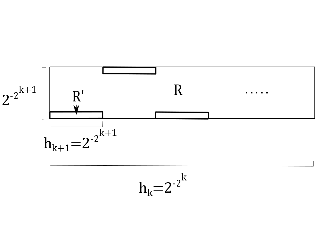
Figure 1: A rectangle $R\in\mathcal{R}_{k}$ and a rectangle $R^{\prime}\in\mathcal{R}_{k+1}$ inside $R$ in Example 5

For Example 6 we choose $n_{k}=1$ and we let $\lambda_{k}=1/2$, when $34M4^{-k}\geq 2^{-k}$, that is, $2^{k}\leq 34M$, and $\lambda_{k}=34M2^{-k-1}$ for all larger $k$. As a consequence, for large enough $k$, the rectangles in $\mathcal{R}_{k}$ have horizontal sides of length $h_{k}=2^{-k}$ and vertical sides of length $34M4^{-k}$. For $R\in\mathcal{R}_{k}$, we have two rectangles $R_{1}$ and $R_{2}$ of $\mathcal{R}_{k+1}$ inside $R$, one along the lower side of $R$ and one along the upper. The distance between these rectangles is $34M4^{-k}-2\cdot 34M4^{-k-1}=17M4^{-k}$ (see Figure 2).

Let $0<r<1$ and let $k$ be such that $2^{1-k}\leq r<2^{2-k}$. We assume that $r$ is small enough so that $2^{k}>68M$. Let $R,R_{1}$ and $R_{2}$ be as above and $p\in R_{2}$. Then $Mr^{2}\leq M4^{2-k}<17M4^{-k}$, whence $R_{1}$ lies outside $V(p)(Mr^{2})$. On the other hand, as $2^{1-k}\leq r$, $R_{1}$ lies inside $B_{E}(p,r)$. This implies that $B_{E}(p,r)\setminus V(p)(Mr^{2})$ contains $R_{1}$, from which the asserted properties follow as in the case of Example 5.

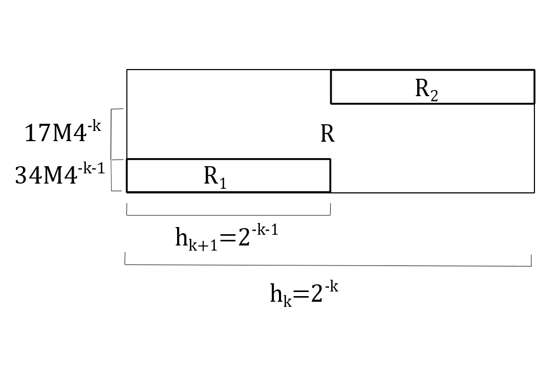
Figure 2: A rectangle $R\in\mathcal{R}_{k}$ and the rectangles $R_{1},R_{2}\in\mathcal{R}_{k+1}$ inside $R$ in Example 6

The next example shows that the conclusion of Theorem 2 fails when $2<s<3$.

Example 7.

For any $2<s<3$ there exist constants $c_{s},\delta_{s}>0$ and a set $F_{s}\subset\mathbb{H}^{1}$ such that $\mathcal{H}^{s}_{E}(F_{s})>0$, $\mathcal{H}^{2s-2}_{H}(F_{s})<\infty$ and for $\mathcal{H}^{s}_{E}$ almost every $p\in F_{s}$,

$$\liminf_{r\rightarrow 0}\frac{\mathcal{H}^{s}_{E}(F_{s}\cap B_{E}(p,r)\setminus V(p)(\delta_{s}r))}{r^{s}}\geq c_{s}.$$ (42)

This example is taken from Theorem 4.1 in [BT], where it is used to show the sharpness of some of the dimension inequalities. We will consider the Heisenberg square $Q_{H}$ and a certain Cantor set above each point of $Q_{H}$. The Heisenberg square is the invariant set of the affine iterated function system $F_{1},F_{2},F_{3},F_{4}$, that is $Q_{H}=\cup_{j=1}^{4}F_{j}(Q_{H})$. The maps $F_{i}:\mathbb{H}^{1}\rightarrow\mathbb{H}^{1}$, $i=1,2,3,4$, are similarities with respect to $d_{H}$ with contraction ratio $1/2$ and they are horizontal lifts of $f_{j}$, $j=1,2,3,4$, which are maps in the plane. This means that $\pi\circ F_{j}=f_{j}\circ\pi$, where $\pi:\mathbb{R}^{3}\rightarrow\mathbb{R}^{2}$ is the projection $\pi(x,y,t)=(x,y)$. These maps have the form $f_{j}(x,y)=\frac{1}{2}((x,y)+v_{j})$, where $v_{1}=(0,0)$, $v_{2}=(1,0)$, $v_{3}=(0,1)$ and $v_{4}=(1,1)$. Then we have $\pi(Q_{H})=Q=[0,1]^{2}$, where $Q$ is the invariant set of the iterated function system $f_{1},f_{2},f_{3},f_{4}$. See [BHT] and [BT] for more details. We will use the symbolic dynamics notation: for $m\geq 1$ and $w=w_{1}w_{2}\dots w_{m}\in W_{m}=\{1,2,3,4\}^{m}$ we let $F_{w}=F_{w_{1}}\circ\dots\circ F_{w_{m}}$. Then $Q_{H}=\cup_{w\in W_{m}}F_{w}(Q_{H})$ for every $m$.

Given $2<s<3$, let $d=s-2$ and let $C_{d}$ be a standard symmetric Cantor set in the $t$-axis such that $0<\mathcal{H}^{d}_{E}(C_{d})<\infty$. Then $0<\mathcal{H}^{2d}_{H}(C_{d})<\infty$. Moreover, $C_{d}$ is $d$-Ahlfors regular, which implies that for $0<r<1$ and $(0,0,t^{\prime})\in C_{d}$,

$$\mathcal{H}^{d}_{E}(\{(0,0,t)\in C_{d}:c_{0}r\leq|t-t^{\prime}|\leq\frac{r}{4}\})\geq c_{d}r^{d}$$ (43)

for some constants $c_{0}$ and $c_{d}$. The set $C_{d}$ is the invariant set associated to two maps $G_{1},G_{2}$, which are $2^{-1/2d}$-Lipschitz with respect to $d_{H}$. Let

$$F_{s}=\{(x,y,t+t^{\prime}):(x,y,t)\in Q_{H},(0,0,t^{\prime})\in C_{d}\}.$$

It is shown in Theorem 4.1 in [BT] that $\mathcal{H}^{s}_{E}(F_{s})>0$ and $\mathcal{H}^{2s-2}_{H}(F_{s})<\infty$.

Let $p=(\bar{x},\bar{y},\bar{t}+\bar{t}^{\prime})\in F_{s}$ and let $0<r<\min\{1/20,c_{0}/6\}$. Let $m$ be the integer such that $2^{-m+2}\operatorname{diam}_{H}(Q_{H})\leq r<2^{-m+3}\operatorname{diam}_{H}(Q_{H})$, then $2^{-m+2}\operatorname{diam}_{H}(Q_{H})<\min\{1/20,c_{0}/6\}$. Let $n$ be the smallest integer such that $n\geq 2dm$. For $w\in\{1,2,3,4\}^{m}$ and $v\in\{1,2\}^{n}$, let

$$F^{vw}_{s}=\{(x,y,t+t^{\prime}):(x,y,t)\in F_{w}(Q_{H}),(0,0,t^{\prime})\in G_{v}(C_{d})\}\subset F_{s}.$$

Then

$$\operatorname{diam}_{H}(F^{vw}_{s})\leq 2^{-m+2}\operatorname{diam}_{H}(Q_{H})\leq r.$$

Indeed, if $\operatorname{diam}_{H}(F^{vw}_{s})=d_{H}((x,y,t+t^{\prime}),(\tilde{x},\tilde{y},\tilde{t}+\tilde{t}^{\prime}))$, then we have, as shown in the proof of Theorem 4.1 in [BT],

$$\operatorname{diam}_{H}(F^{vw}_{s})^{4} =((x-\tilde{x})^{2}+(y-\tilde{y})^{2})^{2}+(t+t^{\prime}-\tilde{t}-\tilde{t}^{\prime}-2(\tilde{x}y-\tilde{y}x))^{2}$$

$$\leq 2(((x-\tilde{x})^{2}+(y-\tilde{y})^{2})^{2}+(t-\tilde{t}-2(\tilde{x}y-\tilde{y}x))^{2}+(t^{\prime}-\tilde{t}^{\prime})^{2})$$

$$\leq 2(2^{-4m}\operatorname{diam}_{H}(Q_{H})^{4}+2^{-2n/d})\leq 2^{-4m+2}\operatorname{diam}_{H}(Q_{H})^{4}.$$

Let $w$ and $v$ be such that $p\in F^{vw}_{s}$, so we have $F^{vw}_{s}\subset F_{s}\cap B_{H}(p,r)$. Let now $q=(x,y,t+t^{\prime})\in F^{vw}_{s}$ be such that $|x-\bar{x}|^{2}+|y-\bar{y}|^{2}\leq r^{2}/400$. Then $q\in B_{H}(p,r)$ and we have

$$|t+t^{\prime}-\bar{t}-\bar{t}^{\prime}| \leq|t+t^{\prime}-\bar{t}-\bar{t}^{\prime}-2(\bar{x}y-\bar{y}x)|+2|\bar{x}y-\bar{y}x|$$

$$\leq d_{H}(p,q)^{2}+2|\bar{x}(y-\bar{y})+(\bar{x}-x)\bar{y}|$$

$$\leq r^{2}+\frac{4r}{20}\leq\frac{r}{20}+\frac{4r}{20}=\frac{r}{4}.$$ (44)

Let

$$C^{q}_{d}=\{(0,0,t^{\prime\prime})\in C_{d}:c_{0}r\leq|t^{\prime\prime}-t^{\prime}|\leq\frac{r}{4}\}.$$ (45)

We want to show that the set

$$L_{q}=\{(x,y,t+t^{\prime\prime}):(0,0,t^{\prime\prime})\in C_{d}^{q}\}$$

is contained in

$$D_{r}=F_{s}\cap B_{E}(p,r)\cap\{(x,y,t):|x-\bar{x}|^{2}+|y-\bar{y}|^{2}\leq r^{2}/400\}\setminus V(p)(c_{0}r/6).$$

Let $q^{\prime\prime}=(x,y,t+t^{\prime\prime})\in L_{q}$. Then $q^{\prime\prime}\in F_{s}$ since $(x,y,t)\in Q_{H}$ and $(0,0,t^{\prime\prime})\in C_{d}$. Moreover, by (4) and (45) we have

$$|t+t^{\prime\prime}-\bar{t}-\bar{t}^{\prime}|\leq|t+t^{\prime}-\bar{t}-\bar{t}^{\prime}|+|t^{\prime\prime}-t^{\prime}|\leq\frac{r}{4}+\frac{r}{4}=\frac{r}{2},$$

thus

$$|q^{\prime\prime}-p|^{2}=|x-\bar{x}|^{2}+|y-\bar{y}|^{2}+|t+t^{\prime\prime}-\bar{t}-\bar{t}^{\prime}|^{2}\leq\frac{r^{2}}{400}+\frac{r^{2}}{4}<r^{2}.$$

This implies that $q^{\prime\prime}\in B_{E}(p,r)$. It remains to show that $d_{E}(q^{\prime\prime},V(p))\geq c_{0}r/6$. Using (4), (45) and the facts that $\bar{x}^{2}+\bar{y}^{2}\leq 2$ and $d_{H}(p,q)\leq r<c_{0}/6$, we have

$$d_{E}(q^{\prime\prime},V(p)) =\frac{|\bar{t}+\bar{t}^{\prime}-t-t^{\prime\prime}-2(x\bar{y}-y\bar{x})|}{\sqrt{1+4(\bar{x}^{2}+\bar{y}^{2}})}$$

$$\geq\frac{|t^{\prime}-t^{\prime\prime}|}{\sqrt{1+4(\bar{x}^{2}+\bar{y}^{2}})}-\frac{|\bar{t}+\bar{t}^{\prime}-t-t^{\prime}-2(x\bar{y}-y\bar{x})|}{\sqrt{1+4(\bar{x}^{2}+\bar{y}^{2}})}$$

$$\geq|t^{\prime}-t^{\prime\prime}|/3-d_{H}(q,p)^{2}\geq c_{0}r/3-r^{2}\geq c_{0}r/6.$$

Hence we have

$$L_{q}\subset D_{r}\subset F_{s}\cap B_{E}(p,r)\setminus V(p)(c_{0}r/6).$$ (46)

In particular, for every point $(x,y,t)\in F_{w}(Q_{H})$ such that $|x-\bar{x}|^{2}+|y-\bar{y}|^{2}\leq r^{2}/400$ there are points $(x,y,t+t^{\prime\prime})\in D_{r}$. Thus

$$\pi(F_{s}\cap B_{E}(p,r)\setminus V(p)(c_{0}r/6)) \supset\pi(D_{r})$$

$$\supset\pi(F_{w}(Q_{H}))\cap\{(x,y):|x-\bar{x}|^{2}+|y-\bar{y}|^{2}\leq r^{2}/400\}$$

$$=f_{w}(Q)\cap\{(x,y):|x-\bar{x}|^{2}+|y-\bar{y}|^{2}\leq r^{2}/400\},$$

which implies

$$\mathcal{H}^{2}_{E}(\pi(D_{r}))\geq\mathcal{H}^{2}_{E}(f_{w}(Q)\cap\{(x,y):|x-\bar{x}|^{2}+|y-\bar{y}|^{2}\leq r^{2}/400\})\geq cr^{2}$$ (47)

for some constant $c$. Then by (46), (43), (47) and Theorem 7.7 in [M] we have for some constant $c^{\prime}>0$,

$$\mathcal{H}^{s}_{E}(F_{s}\cap B_{E}(p,r)\setminus V(p)(c_{0}r/6)) \geq\mathcal{H}^{s}_{E}(D_{r})$$

$$\geq c^{\prime}\int_{\pi(D_{r})}\mathcal{H}^{d}_{E}(\{(0,0,t_{q}+t^{\prime\prime}):q=(x_{q},y_{q},t_{q}+t^{\prime\prime})\in D_{r}\})d\mathcal{H}^{2}_{E}(x_{q},y_{q})$$

$$\geq c^{\prime}\int_{\pi(D_{r})}\mathcal{H}^{d}_{E}(C^{q}_{d})d\mathcal{H}^{2}_{E}(x_{q},y_{q})$$

$$\geq c^{\prime}c_{d}r^{d}\mathcal{H}^{2}_{E}(\pi(D_{r}))\geq c^{\prime}c_{d}cr^{2+d}=c_{s}r^{s},$$

which implies (42).

Department of Mathematics and Statistics, P.O. Box 68, FI-00014 University of Helsinki, Finland,
E-mail addresses: pertti.mattila@helsinki.fi, laura.venieri@helsinki.fi