Galaxy And Mass Assembly (GAMA): The galaxy stellar mass function to $z=0.1$ from the r-band selected equatorial regions.

Abstract

We derive the low redshift galaxy stellar mass function (GSMF), inclusive of dust corrections, for the equatorial Galaxy And Mass Assembly (GAMA) dataset covering 180 deg². We construct the mass function using a density-corrected maximum volume method, using masses corrected for the impact of optically thick and thin dust. We explore the galactic bivariate brightness plane ($M_{\star}-\mu$), demonstrating that surface brightness effects do not systematically bias our mass function measurement above 10^7.5 M_⊙. The galaxy distribution in the $M-\mu$-plane appears well bounded, indicating that no substantial population of massive but diffuse or highly compact galaxies are systematically missed due to the GAMA selection criteria. The GSMF is fit with a double Schechter function, with $\mathcal{M}^{\star}=10^{10.78\pm 0.01\pm 0.20}M_{\odot}$, $\phi^{\star}_{1}=(2.93\pm 0.40)\times 10^{-3}h_{70}^{3}$Mpc^-3, $\alpha_{1}=-0.62\pm 0.03\pm 0.15$, $\phi^{\star}_{2}=(0.63\pm 0.10)\times 10^{-3}h_{70}^{3}$Mpc^-3, and $\alpha_{2}=-1.50\pm 0.01\pm 0.15$. We find the equivalent faint end slope as previously estimated using the GAMA-I sample, although we find a higher value of $\mathcal{M}^{\star}$. Using the full GAMA-II sample, we are able to fit the mass function to masses as low as $10^{7.5}$ $M_{\odot}$, and assess limits to $10^{6.5}$ $M_{\odot}$. Combining GAMA-II with data from G10-COSMOS we are able to comment qualitatively on the shape of the GSMF down to masses as low as $10^{6}$ $M_{\odot}$. Beyond the well known upturn seen in the GSMF at $10^{9.5}$ the distribution appears to maintain a single power-law slope from $10^{9}$ to $10^{6.5}$. We calculate the stellar mass density parameter given our best-estimate GSMF, finding $\Omega_{\star}=1.66^{+0.24}_{-0.23}\pm 0.97h^{-1}_{70}\times 10^{-3}$, inclusive of random and systematic uncertainties.

1 Introduction

The Galaxy Stellar Mass Function (GSMF; Bell et al. 2003; Baldry et al. 2008, 2012) is arguably one of the most fundamental measurements in extra-galactic astronomy. Its integral returns the density of baryonic mass currently bound in stars (and hence the global efficiency of star-formation) while the shape of the distribution describes the evolutionary pathways which have shuffled matter from atomic to stellar form — essentially mergers building the high mass end of the GSMF ($M_{\star}\geq 10^{10.8}$) while in-situ star-formation fueled by gas accretion has built the low mass end (Robotham et al., 2014). Not surprisingly the GSMF is also the key calibration for most galaxy formation models that are carefully tuned to best reproduce the latest GSMF measurement (Schaye et al., 2015; Crain et al., 2015; Lacey et al., 2016; Gonzalez-Perez et al., 2014; Genel et al., 2014). In particular the comparison between observations of the GSMF and numerical simulations of the dark-matter halo mass function have led directly to the notion of feedback — both AGN feedback at high mass (see,  e.g. Bower et al. 2006; Croton et al. 2006) and supernova feedback at low mass (Efstathiou, 2000). These are now core elements of semi-analytic prescriptions used to populate the halos formed in purely dark-matter N-body simulations (Lacey et al., 2016; Gonzalez-Perez et al., 2014).

Observationally the measurement of the GSMF has superseded the earlier focus on the measurements of the galaxy luminosity function. Initially these were undertaken in the optical and later at near-IR wavelengths, where the near-IR light was shown to more closely trace the low mass stellar populations that dominate the stellar mass repository. Near-IR is the best single-band proxy for stellar mass because near-IR colours contain little information about mass-to-light variations. This conspires to mean there is less scatter in near-IR single-band mass-to-light estimates compared to the same proxies measured in the optical. Once multi-band optical and NIR data became ubiquitous, however, better estimates could be obtained by making use of full SED colour information. Ultimately a lot of information on optical mass-to-light is contained in the restframe g-r-i colours, so surveys such as SDSS and GAMA could make estimates of stellar mass content that are accurate within $<0.2$ dex (Taylor et al., 2011). Over the past two decades the ability to estimate stellar mass has also become more established (see,  e.g. Bell et al. 2007; Kauffmann et al. 2003; Taylor et al. 2011). As a consequence effort has now shifted from measuring galaxy luminosity functions to the GSMF. The most notable measurements are those deriving from large redshift surveys, in particular the 2dF Galaxy Redshift Survey (2dFGRS; Cole et al. 2001), the Sloan Digital Sky Survey (SDSS; Bell et al. 2003; Baldry et al. 2008), the Millennium Galaxy Catalogue (MGC; Driver et al. 2007), and the Galaxy And Mass Assembly Survey (GAMA; Baldry et al. 2012). In general there is a reasonable consensus with the latest measurement from the GAMA team (Baldry et al., 2012), probing to a stellar mass limit of $10^{8}$M_⊙.

However three key observational concerns remain: susceptibility to surface brightness selection effects, the impact of dust attenuation, and the prospect of a sharp upturn in the space density at very low stellar masses (i.e., below the current observational mass limits). All three effects could potentially lead to underestimating the GSMF and the corresponding stellar mass density. This is particularly significant when looking to reconcile the current stellar mass density with the integral of the cosmic star-formation history (CSFH; see Wilkins et al. 2008a; Baldry & Glazebrook 2003), where a significant discrepancy was seen. In an attempt to explain this discrepancy, some studies have invoked either a top-heavy IMF (which produces more luminosity per unit mass of stars; Baldry & Glazebrook 2003), a time varying IMF (Wilkins et al., 2008b; Ferreras et al., 2015; Gunawardhana et al., 2011), distinct IMFs for bulge (closed-box star-formation with a top-heavy IMF) and disc formation (infall star-formation with a standard Chabrier-like IMF) as proposed by Lacey et al. (2016), or an IMF with a larger fraction of returned mass ( e.g. Maraston 2005; see also Madau & Dickinson 2014). Additionally, the integrated cosmic star-formation history will tend to capture all star formation events without consideration of dynamical interactions that deposit formed stars into the intra-halo medium (IHM). This means that the integrated cosmic star-formation history naturally includes stellar material not currently bound to observed galaxies. The combination of the CSFH and the GSMF measured across a broad redshift range is therefore a powerful tool to constrain the IMF, feedback and extraneous material stripped from galaxies.

The first comprehensive measurements of the GSMF were made by Cole et al. (2001). This was based on the combination of spectroscopic measurements from the 2dFGRS combined with photometric near-IR measurements from 2MASS. Concurrently, Kochanek et al. (2001) also used 2MASS to estimate the value of $\Omega_{\star}$ from K-band luminosity function, although did not calculate the GSMF explicitly. Andreon (2002) subsequently demonstrated that the shallow 2MASS survey misses dim galaxies entirely and significantly underestimated the fluxes of late-type systems. Similarly the later and larger studies based on SDSS and GAMA are both reliant on the completeness of the spectroscopic input catalogues derived from (relatively) shallow drift-scan SDSS imaging. Blanton et al. (2005) demonstrated, via adding simulated galaxies to SDSS data, that incompleteness in the imaging and spectroscopy can become severe for systems with average surface brightnesses of $\mu_{50,r}\approx 23.5$mag/sq arcsec (see Figure $2$ of Blanton et al. 2005, and Figure $11$ of Baldry et al. 2012). However one indication that the surface brightness problem may not be overly severe comes from deep field studies (see,  e.g. Driver 1999), novel analysis methods designed to search for low-surface brightness galaxies in wide-field imaging (Williams et al., 2016), and dedicated low-surface brightness studies (see,  e.g. Davies et al. 2016; Geller et al. 2012), which generally found that large populations of low surface brightness systems do not contribute significantly to the stellar mass density. Furthermore, attempts to correct galaxy luminosity function estimates via a bivariate brightness analysis also failed to find extensive populations of low surface brightness giant galaxies (see,  e.g. Cross et al. 2001; Driver et al. 2005).

Dust attenuation has perhaps a more subtle effect. Generally dust will both diminish and redden a galaxy’s emission, and these two effects arguably cancel — the reduction in total light is compensated for by an increase in the estimated mass-to-light ratio (see,  e.g. the vector shown in Figure 6 of Bell et al. 2003, and Figure 11 of Taylor et al. 2011). Strictly this is only true in the optically thin case, as if no light from a particular region is able to escape then the loss of flux cannot be recovered. The MGC team (Driver et al., 2007) attempted to quantify the impact of dust attenuation on galaxy mass estimates by measuring the shift in the recovered ${\mathcal{M}}^{\star}$-parameter of the optical $B$-band luminosity function with systemic inclination. The implicit assumption was that, if dust attenuation is significant, edge-on systems should be more attenuated than their face-on counterparts. A significant $M_{\star}-cos(i)$ effect was seen (Driver et al., 2007) which, following extensive modelling using radiative transfer codes (Tuffs et al., 2004; Popescu et al., 2000), suggested that the average face-on central opacity of galaxy discs was $\tau_{v}=3.8$;  i.e. the centres of galaxies are optically thick. The resulting impact, based on corrections using the radiative transfer models, was to increase the estimate of the present day integrated stellar mass density from $\sim 5\%$ (Baldry et al., 2008) to $\sim 8\%$ (Driver et al., 2007). However significant concerns remain as to the validity of adopting a constant central face-on opacity for all galaxy types. Indeed, direct observations of galaxies have indicated that the intrinsic nature of dust in galaxies is highly variable, depending on multiple factors such as morphology and environment (see,  e.g. , White et al. 2000; Keel & White 2001; Holwerda 2005; Holwerda et al. 2013a; Holwerda et al. 2013b).

Measurements of the GSMF to date reliably extend only to $10^{8}$M_⊙ whereas we have proof-of-existence of galaxies with masses as low as $10^{3}$M_⊙ in the Local Group (McConnachie, 2012). Hence there is also some uncertainty as to whether an extrapolation of the GSMF from $10^{8}$M_⊙ to $10^{3}$M_⊙ is valid. Recently the study by Moffett et al. (2016), where the stellar mass functions was divided by galaxy type, showed two populations with very rapidly rising slopes at the mass-limit boundary.

All three areas (surface brightness, dust attenuation, and low mass systems) have the potential to bring into question the robustness of our current estimates of the GSMF and the integrated cosmic stellar mass density. In this paper we provide an updated GSMF, defined using the SDSS r-band, for the completed Galaxy And Mass Assembly (GAMA; Driver et al. 2011; Liske et al. 2015) survey equatorial fields.

In Section 2, we introduce the GAMA–II sample which is approximately double the size of the GAMA–I sample used in Baldry et al. (2012), extending 0.4mag deeper (to $r=19.8$mag) and over an expanded area of 180 sq deg. We also utilise the full GAMA panchromatic imaging dataset (Driver et al., 2016b), and photometry measured consistently in all bandpasses from far-UV to far-IR (Wright et al., 2016). The far-IR data from Herschel ATLAS (Eales et al., 2010) in particular allow for full SED modelling using codes such as magphys (da Cunha et al., 2008; da Cunha & Charlot, 2011), which accounts for dust attenuation and re-emission when calculating stellar masses. In Section 3 we compare the stellar masses derived from optical data using stellar template modelling (Taylor et al., 2011) to those derived via the full SED modelling from magphys. In Section 4, we derive our base GSMF, incorporating density modelling of the GAMA volumes. In Section 5 we revert to a simpler empirical 1/V_max method applied in the bivariate brightness plane to specifically explore the possible impact of surface brightness selection bias. Finally in Section 6 we include similar photometric data from the G10-COSMOS regions (Davies et al., 2015a; Andrews et. al., 2016), fit with magphys (Driver et al., 2016b) using high precision photometric redshifts from Laigle et al. (2016), to provide an indication as to the possible form of the stellar mass function to very low stellar masses ($10^{6}$M_⊙). We discuss our results in Section 7. Throughout this work we use a standard concordance cosmology of $\Omega_{M}=0.3$, $\Omega_{\Lambda}=0.7$, $H_{o}=70$ kms^-1Mpc^-1, and $h_{70}=H_{o}/70$ kms^-1Mpc^-1. We implement a standard Chabrier (2003) IMF, and all magnitudes are presented in the AB system.

2 Data and Sample Definition

The Galaxy And Mass Assembly (GAMA; Baldry et al. 2010; Driver et al. 2011; Liske et al. 2015; Hopkins et al. 2013) survey is a large multi-wavelength dataset built upon a spectroscopic campaign aimed at measuring redshifts for galaxies with $r<19.8$ mag at $>98\%$ completeness (Robotham et al., 2010). The survey’s complementary multi-wavelength imaging is in 21 broadband photometric filters (Driver et al., 2016b) spanning from the far-UV (FUV) to the far-IR (FIR). Given this wealth of broadband imaging, we are able to calculate matched photometry for the purposes of estimating galaxy stellar masses. We use 21-band photometry contained in the GAMA lambdar Data Release (LDR), presented in Wright et al. (2016). The LDR photometry is deblended matched aperture photometry accounting for each image’s pixel resolution and point spread function. Apertures used in lambdar are defined using a mixture of source extractions on the SDSS r-band, source extractions on the VISTA Z-band, and by-hand definitions using VISTA Z-band images. Measurements are made for all images in the GAMA Panchromatic Data Release (Driver et al., 2016b).

This photometric dataset is designed specifically for use in calculating spectral energy distributions (SEDs), as the photometry and uncertainties are consistently measured across all passbands. Furthermore, as the photometry is matched aperture, there exists an estimate in every band for every object in the sample, with a corresponding uncertainty (except, of course, where there is no imaging data available due to coverage gaps). For the calculation of relevant cosmological distance parameters and redshift limits, fluxes have been appropriately k-corrected using KCorrect (Blanton & Roweis, 2007), and redshifts have been flow-corrected using using the models of Tonry et al. (2000) as described in Baldry et al. (2012).

We calculate stellar masses for the LDR photometry using two independent methods. Firstly, we fit panchromatic SEDs to the full 21-band dataset using the energy balance program magphys (da Cunha et al., 2008; da Cunha & Charlot, 2011). A full description of the magphys fits to the GAMA LDR is provided in Driver et. al. (2016a). magphys utilises information from the UV to the FIR to estimate the total stellar mass of each galaxy from both visible and obscured stars, assuming Bruzual & Charlot (2003) (BC03) models, a Chabrier (2003) initial mass function (IMF), and the Charlot & Fall (2000) dust obscuration law. Secondly, we use the measurement of Taylor et al. (2011) who estimated stellar masses by fitting a comprehensive grid of SED templates to photometry from the SDSS $u$-band to the VIKING $K_{s}$-band, applied to our updated LDR photometry. Their technique uses stellar population synthesis models with exponentially declining star-formation histories, without bursts, and the same BC03 models and Chabrier (2003) IMF as magphys, but uses a Calzetti et al. (2000) dust obscuration law. In addition to this difference in implemented dust obscuration law, the predominant differences between these two methods are:

• the wider range of photometric filters (and energy balance) used in magphys;

• the incorporation of bursty star-formation histories in magphys;

• a sparser grid of star formation histories in magphys.

For clarity, throughout this work we refer to stellar mass estimates from magphys, which utilise the full far-UV to far-IR bandpass, as ‘bolometric’ masses, and stellar masses from our stellar population synthesis templates, which are fit across the near-UV to near-IR passbands, as ‘optical’ masses.

Using these two methods, we check for systematic differences in our estimated stellar masses. By comparing the two sets of mass estimates, we can explore how our subsequent fits are systematically affected by our choice of stellar mass estimation. In particular, an observed difference in the mass estimates (and GSMF fits) can indicate the impact of optically thick dust on our masses (as magphys includes consideration of optically thick dust, whereas our optically estimated masses do not).

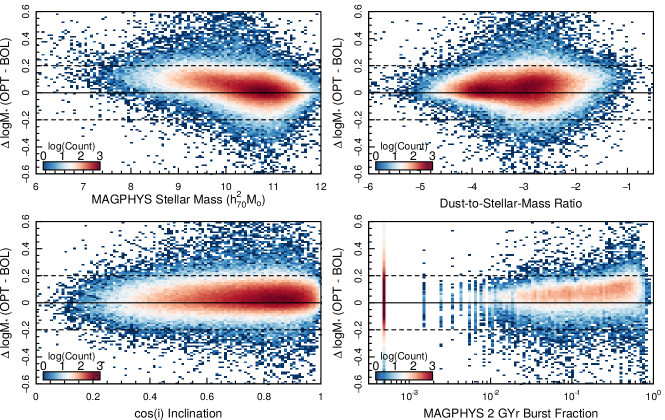
Figure 1: Comparison of bolometric stellar masses returned by magphys to those measured using the optical-only method presented in Taylor et al. (2011), as a function of magphys stellar mass (panel ‘a’), magphys dust mass (panel ‘b’), galaxy inclination (panel ‘c’), and magphys burst fraction over the last 2 Gyr (panel ‘d’). While all of these figures show typical agreement within $\pm 0.2$ dex, there are systematic trends visible in each distribution which we attribute to the difference in chosen dust attenuation and burst models between the codes.

Figure 1 shows a compendium of the four main comparison planes that demonstrate systematic differences; namely variations as a function of stellar mass (upper left), dust-to-stellar mass ratio (upper right), galaxy inclination (lower left), and magphys burst fraction over the last 2 Gyr (lower right). We note that there are two populations that separate out in the upper panels, most notably in the dust-to-stellar mass ratio comparison. The most systematically different stellar masses are localised at small stellar masses, high dust-to-stellar mass ratios, and at higher magphys burst fraction. Each of these properties is consistent with belonging to the predominantly young and disc-dominated portion of the sample, where bursts and variations in the dust obscuration prescription are likely to have the most impact. As a result, we postulate that the differences seen in the mass estimates stem predominantly from the differences in libraries, models, and burst prescriptions implemented in our fitting procedures. However despite these visible differences, we find that $94.8\%$ of the sample are contained within $\lvert{\Delta\log_{10}M}\rvert\leq 0.2$ for the entire sample. This fraction increases to $97.8\%$ if we select only masses with magphys goodness-of-fit $0.5\leq\chi_{\nu}^{2}\leq 1.5$. For the low redshift portion of the data ($0.002<z<0.1$), there are $86.0\%$ of masses within $\lvert{\Delta\log_{10}M}\rvert\leq 0.2$, and $88.8\%$ when selecting $0.5\leq\chi_{\nu}^{2}\leq 1.5$. In general, the optically derived masses return slightly higher stellar masses (median offset $\Delta\log_{10}M=\log_{10}M_{\rm OPT}-M_{\rm BOL}=0.03$) than the bolometrically modelled masses, and (as there is no obvious trend in inclination) there appears to be no indication of significant quantities of optically thick dust. All of these systematic shifts in masses are well within both the typical quoted mass uncertainty (median mass uncertainty $\delta\log_{10}M=0.10$), and within the width of the central $68^{\rm th}$ percent range ( i.e. $1\sigma$) of the distribution ($\sigma_{M}=0.14$).

Finally, we implement a correction to account for flux/mass missed by the matched aperture photometry described in Wright et al. (2016). To correct for systematically missed flux/mass, we utilise the GAMA Sersic profile fits to our sample. We calculate the linear ratio between the measured Sersic flux and aperture flux for each source (this is the same aperture correction described in Taylor et al. 2011, and is often referred to as the ‘fluxscale’ factor in GAMA data products and publications). This correction has the effect of preferentially boosting high-mass sources, as stellar mass is loosely correlated with galaxy Sersic index n and (in a fixed finite aperture) galaxies will increasingly miss flux with increasing n. However, as this correction is based on the empirically estimated Sersic fits (which are themselves possibly subjected to random and systematic biases), we provide the results for the uncorrected masses in Appendix A. These fits provide lower limits for the various parameters estimated in this work.

2.1 Additional systematic biases

By estimating our stellar masses using our ‘optical’ and ‘bolometric’ methods, we attempt to explore how the stellar mass function is affected by some of the choices and assumptions that have been made in this work (such as the impact of dust and the allowed burstiness). However these tests certainly do not encompass the full gambit of assumptions implicit to stellar mass estimation using stellar population synthesis (SPS) models. Such assumptions are required because of our uncertainty of, for example, the stellar initial mass function (Driver et al., 2012), the contribution of thermally-pulsing asymptotic giant branch (TP-AGB) stars (Maraston, 2005; Bruzual, 2007; Conroy et al., 2009), the choice of parametrization of star formation histories (Fontana et al., 2004; Pacifici et al., 2015), modelling of bursts (Pozzetti et al., 2007), and more. Here we briefly discuss the effect of some of these assumptions, and derive an estimate of the systematic uncertainty required to be added to our estimates of stellar masses and their derived quantities.

Systematic effects originating from our uncertainty in the stellar IMF are well documented in the literature, and there is an ongoing debate as to whether the shape of the initial mass function is well described by something akin to the Chabrier (2003) IMF, or whether it is better described by a top-heavy (Baldry & Glazebrook, 2003) or bottom-heavy (Kroupa et al., 1993) function, or whether there is a single valid description for the IMF over all times (Wilkins et al., 2008a). Generally, variation of the IMF manifests itself as a shift in the stellar population mass-to-light ratio, and thus as a scaling of the estimated mass of each galaxy, as the IMFs typically differ in their treatment of only the most and least massive stars (Bell et al., 2003; Driver, 2013). This, in turn, means that a change in the IMF will cause a multiplicative scaling of estimated quantities such as $\mathcal{M}_{\star}$ and $\Omega_{\star}$. Driver et al. (2012) provided a prescription for converting between some of the various popular IMFs in the literature, which we reproduce here in Table 1. By providing this table we wish to emphasise that the estimates of $\mathcal{M}_{\star}$ and $\Omega_{\star}$ provided in this work are valid only for the Chabrier (2003) IMF, and that these values are highly sensitive to the choice of IMF. Nonetheless, in the case where the variation in the IMF can be well described by a multiplicative scaling of overall stellar mass, Table 1 should allow the conversion of our estimated parameters between the Chabrier (2003) and other popular IMFs. Note that as these corrections are only valid in the case of a single non-evolving IMF, or when analysing galaxies over a fixed epoch (Conroy et al., 2009).

IMF	$M_{\star}/M_{\star,Ch}$
Salpeter (1955)	1.53
Kroupa et al. (1993)	2.0
Kroupa (2001)	1.0
Chabrier (2003)	1.0
Baldry & Glazebrook (2003)	0.82
Hopkins & Beacom (2006)	1.18

Table 1: Multiplicative factors for converting between stellar masses and mass densities that are estimated using different initial mass functions, relative to the Chabrier (2003) IMF used in this work.

In addition to the uncertainty about the shape of the IMF, additional SPS uncertainties can lead to significant systematic biases in stellar mass estimation. Conroy et al. (2009) provide a detailed discussion of uncertainties in SPS masses related to, in particular, TP-AGB stars, horizontal branch stars, and blue straggler stars. Each of these populations are poorly constrained in SPS models, due to their rarity and difficulty to constrain observationally. Conroy et al. (2009) conclude that the typical uncertainty on their mass estimates at $z\sim 0$ range from $\sim 0.1$ dex to $\sim 0.4$ dex, at $95\%$ confidence and for a range of galaxy colours and magnitudes, due to uncertainty in each of these parameters. Furthermore, this uncertainty is not restricted to stellar masses estimated using SPS models. Gallazzi & Bell (2009) show that, using either spectral or photometric estimates of stellar mass-to-light ratios, one can reach a limiting accuracy of only $\sim 0.15$ dex in the regime where a galaxy has undergone recent bursts of star formation. Galaxies with more passive histories can be more accurately constrained in their study; the highest signal-to-noise sources which, are dominated by an old stellar population, having constraints better than 0.05 dex (albeit without consideration of the effects of TP-AGB or HB stars, nor the impact of dust).

Given these systematic biases in estimating stellar mass, it is therefore necessary to encode our systematic uncertainty into our results, separate from the uncertainty due to our fitting and sample. Therefore, throughout this work we will consistently provide two uncertainties on each of our estimates of $\mathcal{M}_{\star}$ and $\Omega_{\star}$;  i.e. $\Omega_{\star}={\rm Val}\pm\sigma_{\rm fit}\pm\sigma_{\rm sys}$. Here $\sigma_{\rm fit}$ is the uncertainty due to our sample and fitting procedure, and incorporates both random uncertainty due to the fit optimisation (discussed further in Section 3.4), and the uncertainty due to cosmic variance (where relevant). For the parameter $\sigma_{\rm sys}$ we choose a fairly conservative $0.2$ dex ($58\%$) uncertainty, encompassing those expected by both Conroy et al. (2009) and Gallazzi & Bell (2009). This value is large, easily dominating over uncertainties quoted on $\mathcal{M}_{\star}$ and $\Omega_{\star}$ in previous works that did not incorporate a quantification of this uncertainty. This is an indication that the uncertainty on our measurement is likely to be dominated by these systematics, and that improvement in the estimation of $\Omega_{\star}$ in particular will be limited by the reduction of uncertainty of stellar mass modelling in the future.

Finally, we also quantify the systematic uncertainty on the Schechter function slope parameters $\alpha_{1}$ and $\alpha_{2}$ (see Section 3.1). While a constant systematic bias in stellar mass will not cause a change in the Schechter function slope, a mass-dependent systematic bias may have this effect. To quantify the slope systematic uncertainty we measure the change in mass function slope when applying a mass dependent systematic bias of the form $M_{\star,\rm sys}=0.95\times M_{\star}+C_{1}$ and $M_{\star,\rm sys}=1.05\times M_{\star}+C_{2}$, where the constants $C_{1}$ and $C_{2}$ are chosen such that $\langle M_{\star,\rm sys}\rangle=\langle M_{\star}\rangle$. These functions bias our stellar masses by $\Delta M_{\star}>0.2$ dex across the mass range of our sample, and so simulate a mass dependent systematic bias on the same scale as the (conservative) systematic mass bias we adopted for $\mathcal{M}_{\star}$ and $\Omega_{\star}$. Fits to these biased masses do exhibit a change in the Schechter function slope parameters, and indicate a conservative systematic uncertainty on $\alpha$ is $\sigma_{\rm sys}=0.15$. We adopt this value for the remainder of this work.

3 The Density-Corrected Maximum-Volume GSMF

Our primary method to calculate the GSMF uses a density-corrected maximum-volume (DCMV) weighting to determine the number density distribution of sources, corrected for absolute-magnitude based observational biases ( i.e. Malmquist (1922) bias). The typical maximum-volume corrected number density (Schmidt, 1968) is calculated by weighting each galaxy by the inverse of the comoving volume over which the galaxy would be visible, given the magnitude limit of the sample, $1/V_{\rm max,i}$. Saunders et al. (1990) and Cole (2011) extend this method to correct for the presence of over- and under-densities in the radial density distribution caused by large-scale structure. This is done by defining a fiducial density between two redshift limits $z_{a}$ and $z_{b}$, and using the ratio of instantaneous density to fiducial density to weight sources, thus avoiding bias due to over- and under-densities caused by large-scale structure. Weigel et al. (2016) showed that this method is robust to observational biases, and indeed returns fits equivalent to those returned by more complex methods, such as the stepwise maximum likelihood method described by Efstathiou et al. (1988).

The DCMV GSMF is defined by first calculating an individual weight for each source in our sample. The DCMV weight per object is

$$W_{i}=\left(V^{\prime}_{\rm max}\right)^{-1}=\left[\frac{1}{V_{\rm max}}\frac{\langle\delta_{f}\rangle}{\delta_{i}}\right],$$ (1)

where $V_{\rm max}$ is the standard maximum-volume factor from Schmidt (1968), $\delta_{i}$ is the instantaneous running density of galaxies at the redshift of galaxy $i$, and $\langle\delta_{f}\rangle$ is the average density of a chosen fiducial population. In this work, we define this fiducial average density $\langle\delta_{f}\rangle$ using the sample of GAMA targets with $M_{\star}>10^{10}M_{\odot}$ and $0.07<z<0.19$. We choose this sample because it exhibits a fairly uniform density, is not affected by incompleteness, and is affected by cosmic variance at the $<10\%$ level (using the cosmic variance estimator of Driver & Robotham 2010; accessible at cosmocalc.icrar.org). Nonetheless, cosmic-variance remains a non-negligible source of uncertainty and therefore is incorporated into all relevant parameter estimates. Panel (a) of Figure 2 shows the relative cumulative density of each of the 3 GAMA equatorial fields, and the region over which our fiducial density is determined. Similarly, Panel (b) shows the differential running density of each field. Finally, panel (c) shows the fiducial sample in mass-redshift space, and shows that the sample is complete in this redshift range.

The cumulative density distributions of each GAMA equatorial field indicate that, integrating the number density out to $z=0.1$, G12 is over-dense relative to our fiducial density by a factor of $1.02$, while G09 and G15 are under-dense relative to our fiducial density by a factor of $1.36$ and $1.22$ respectively. This inter-field variation is in good agreement with the expected cosmic variance between the GAMA fields, which is $\sim 23\%$ per field using the cosmic variance estimator of Driver & Robotham (2010).

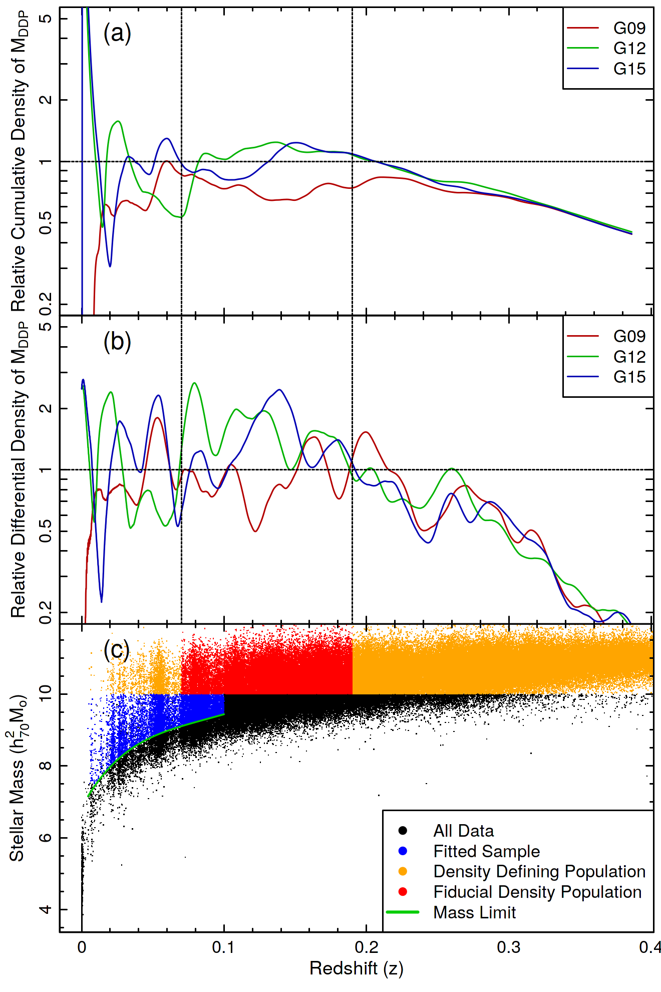
Figure 2: The running density of the GAMA data in each of the 3 equatorial GAMA fields. Panel (a) shows the individual cumulative densities of each field separately, relative to the fiducial density. Panel (b) shows the relative differential density of each field. In the first two panels, the dotted vertical lines mark the redshift boundaries of our fiducial sample. Panel (c) shows the distribution of stellar mass against redshift, with the sample used for estimating the fiducial density highlighted in red, the density defining population in orange, and our low-z mass-limited sample highlighted in blue. The green line shows our mass-limit function used in fitting the GSMF. From these distributions, we conclude that the fiducial sample is not adversely impacted by substantial stellar mass incompleteness or variations in density.

3.1 Schechter function formalism

In this work we will fit mass functions to a range of samples. For this, we elect to use a 2-component Schechter (1976) function. The Schechter function is a specialised form of the logarithmic truncated generalised gamma distribution (TGGD; Murray et. al. prep):

$$\Gamma^{t}(x;\alpha,\beta,s,m)=\frac{\log\left(10\right)\beta\left(10^{\left(x-s\right)}\right)^{\alpha+1}\exp\left(-10^{\left(\beta\left(x-s\right)\right)}\right)}{s\Gamma\left(\frac{\alpha+1}{\beta},\left(10^{(m-s)}\right)^{\beta}\right)},$$ (2)

where $\Gamma$ is the incomplete upper gamma distribution, $\alpha$ is the power-law slope of the TGGD, $\beta$ is the rate of exponential cut-off of the TGGD, $s$ is the scale factor that determines the transition point between the power-law and exponential regimes, and $m$ is the lower-limit that defines the truncation point of the TGGD. The TGGD reduces to the standard Schechter function when $\beta=1$, and (in this form) the TGGD parameters $\alpha$ and $s$ reduce to the normal Schechter parameters $\alpha$ and ${\mathcal{M}}^{\star}$, and we define $m$ to be the minimum mass used in our sample ${M}_{\star}^{\rm min}$ ;

$$S(M;{\mathcal{M}}^{\star},\alpha,M_{\star}^{\rm min})\sim\Gamma^{t}\left(M;\alpha,1,{\mathcal{M}}^{\star},M_{\star}^{\rm min}\right).$$ (3)

As we are using the logarithmic TGGD, masses $M$, ${\mathcal{M}}^{\star}$, and $M_{\star}^{\rm min}$ are all assumed to be logarithmic also. We choose to formulate the Schechter function in this way ( i.e. described using the specialised form of the logarithmic TGGD, rather than using a directly defined Schechter function) as the TGGD is a fully analytic PDF, where the normalisation parameter is able to be evaluated at arbitrary $\alpha$ and ${\mathcal{M}}^{\star}$ as:

$$\phi^{\star}=\frac{\Gamma^{t}\left({\mathcal{M}}^{\star};\alpha,1,{\mathcal{M}}^{\star},M_{\star}^{\rm min}\right)}{\log\left(10\right)\exp\left(-1\right)}.$$ (4)

Thus this formulation does not require any (often CPU intensive) numerical integration to estimate the function normalisation. Using the TGGD to describe the single Schechter function, we define the double Schechter as the sum of two single Schechter functions, with a fractional contribution of component 1, $f_{\rm mix}$, integrated down to $M_{\star}^{\rm min}$:

$$S^{d}(M;{\mathcal{M}}^{\star},\alpha_{1},\alpha_{2},f_{\rm mix},{M}_{\star}^{\rm min})=\\ S\left(M;{\mathcal{M}}^{\star},\alpha_{1},{M}_{\star}^{\rm min}\right)\times f_{\rm mix}+\\ S\left(M;{\mathcal{M}}^{\star},\alpha_{2},{M}_{\star}^{\rm min}\right)\times\left(1-f_{mix}\right).$$ (5)

The double Schechter function is useful for fitting distributions that are expected to contain multiple components, but which we elect to fit with a coupled ${\mathcal{M}}^{\star}$. This has become somewhat common practice in the literature (see,  e.g. , Peng et al. (2010); Baldry et al. (2012); Eckert et al. (2016)), and we follow this procedure as it enables us to more readily compare our results with these previous GSMF estimates.Nonetheless, fits with a decoupled ${\mathcal{M}}^{\star}$ have merit, and can encode interesting physics (see,  e.g. , Kelvin et al. 2014; Moffett et al. 2016). We therefore opt to include the decoupled GSMF fits in Appendix B, for examination by the interested reader.

Our formulated distribution can then be fit to individual data in two ways: by specifying individual weights based on some relevant criteria ( e.g. density corrected maximum volume weights) and fitting over a fixed mass range, or by defining an expected limiting stellar mass ${M}_{\rm\star,i}^{\rm lim}$ per source ( e.g. where observational incompleteness becomes important for that source, in the mass plane). In the latter case, the log-likelihood of each source is then calculated with consideration of the limiting stellar mass of that source given the shape of the Schechter function at that iteration. In this way, the latter procedure includes information of the mass function in the optimisation process in a more considered fashion than the former (the optimisation method is discussed in Section 3.3). We therefore fit our distributions using the mass limit optimisation procedure, whereby we define limits using an analytic expression similar to that of Moffett et al. (2016), but modified to match this sample of masses (see Section 3.2). Note, however, that as we no longer have a single fixed mass limit, our mixture fraction $f_{\rm mix}$ must now be modified per object to reflect the effective mixture fraction given each individual source’s mass limit, $f_{\rm mix,i}$:

$$I^{\rm mix}_{\rm 1,i}=f_{\rm mix}\times\int\limits_{\rm M_{\star}^{\rm min}}^{M_{\rm\star,i}^{\rm lim}}\!\!\!\!S\left(M;{\mathcal{M}}^{\star},\alpha_{1},M_{\star}^{\rm min}\right){\rm d}M,$$ (6)

$$I^{\rm mix}_{\rm 2,i}=\left(1-f_{\rm mix}\right)\times\int\limits_{\rm M_{\star}^{\rm min}}^{M_{\rm\star,i}^{\rm lim}}\!\!\!\!S\left(M;{\mathcal{M}}^{\star},\alpha_{2},M_{\star}^{\rm min}\right){\rm d}M,$$ (7)

$$f_{\rm mix,i}=\frac{I^{\rm mix}_{\rm 1,i}}{I^{\rm mix}_{\rm 1,i}+I^{\rm mix}_{\rm 2,i}}.$$ (8)

Using these individualised limits and mixture fractions, we define the log-likelihood of our fit:

$${\rm ln\mathcal{L}}=\displaystyle\sum\limits_{i}\log\left[S^{d}\left(M_{i};{\mathcal{M}}^{\star},\alpha_{1},\alpha_{2},f_{\rm mix,i},M_{\rm\star,i}^{\rm lim}\right)\right]\times\frac{\delta_{i}}{\langle\delta_{f}\rangle},$$ (9)

and optimise simultaneously for ${\mathcal{M}}^{\star}$, $\alpha_{1}$, $\alpha_{2}$, and $f_{\rm mix}$. The primary benefit of implementing the mass limits in this way is that it at no point requires binning of the data in any form. After this optimisation, we can calculate the values of $\phi^{\star}_{1}$ and $\phi^{\star}_{2}$ using the fit parameters and the defined fiducial population number density, recognising that the ratio of $\phi^{\star}$ values is directly proportional to the integral of the individual Schechter components:

$$I^{\rm mix}_{\rm 1}=f_{\rm mix}\times\int\limits_{\rm M_{\star}^{\rm min}}^{\inf}\!\!\!\!S\left(M;{\mathcal{M}}^{\star},\alpha_{1},{M}_{\star}^{\rm min}\right){\rm d}M,$$ (10)

$$I^{\rm mix}_{\rm 2,i}=\left(1-f_{\rm mix}\right)\times\int\limits_{\rm{M}_{\star}^{\rm min}}^{\inf}\!\!\!\!S\left(M;{\mathcal{M}}^{\star},\alpha_{2},{M}_{\star}^{\rm min}\right){\rm d}M,$$ (11)

$$\frac{\phi^{\star}_{1}}{\phi^{\star}_{2}}=\frac{I^{\rm mix}_{\rm 1}}{I^{\rm mix}_{\rm 2}}.$$ (12)

3.2 Defining Mass Limits

Our mass limit function is shown graphically as the green line in panel ‘c’ of Figure 2 and is known to exhibit $>97\%$ completeness for all sources in GAMA out to $z=0.1$, without biases in mass and/or colour. The process for defining these limits typically involves visually inspecting the distribution of stellar masses as a function of redshift (and vice versa) and determining the point at which the sample begins to become incomplete. Once this has been done in a series of bins of stellar mass and redshift, a polynomial is then fit to the limits.

However, this process is liable to be biased by the eye of the person estimating the limits ( i.e. no two people will be likely to estimate the same limits), and as such we implement automated methods for determining mass limits. The MassFuncFitR package contains a function that performs the above in an automated manner, by estimating the turn-over point of the number density distribution in bins of comoving distance and stellar mass independently. In each bin of comoving distance, the function takes the mass at the peak density as the turn over point, and in bins of stellar mass the function takes the largest comoving distance at median stellar mass density as the turn-over point. Additionally, there is the option to bootstrap this estimation procedure to refine the limits. Indeed, testing of this automated procedure indicates that it is less prone to the introduction of biases than occurs when fitting for mass limits by hand/eye, and produces a sample that is not biased with respect to colour (see Appendix C).

3.3 Optimisation procedures

Once we have our per-object weights, we are able to both visualise and fit the GSMF. For our fits, we utilise a Markov-chain Monte-Carlo (MCMC). For our MCMC optimisation, we calculate the best-fit Schechter function parameters by sampling from the joint posterior-space of the ${\mathcal{M}}^{\star}$, $\alpha_{1}$, $\alpha_{2}$, and $f_{\rm mix}$ parameters. To do this we first assign priors to each parameter; we choose to use uniform priors over the regions $\log_{10}{\mathcal{M}}^{\star}\in[8,11.6]$, $\alpha_{1,2}\in[-2.5,1.5]$, and $f_{\rm mix}\in[0,1]$. Given these priors, evaluated at some sample point, $V_{p}(\log_{10}{\mathcal{M}}^{\star},\alpha_{1},\alpha_{2},f_{\rm mix})$, we can then evaluate the log-posterior as:

$${\rm ln}{\mathcal{P}}={\rm ln}{V_{p}}+{\rm ln}{\mathcal{L}}$$ (13)

where ${\rm ln}{\mathcal{L}}$ is the same as in Equation 9. We sample the posterior space using an Independence Metropolis sampler, and examine the posterior covariances directly to check for stability. For our MCMC, we utilise the Laplace’s Demon package in R, available on the Comprehensive R Archive Network (CRAN). Once we have optimised these parameters, we fit for the total mass function normalisation at ${\mathcal{M}}^{\star}$, and use the $f_{\rm mix}$ parameter to determine the fractional contributions from each component, thus determining the two $\phi^{\star}$ parameters. We then utilise the full posterior distribution to estimate the uncertainty on each of our $\phi^{\star}$ values, incorporating consideration for the covariances between parameters.

3.4 Verifying fit uncertainties

In order to verify that the uncertainties from our MCMC are a true reflection of the data, we perform 100 Jackknife resamplings of the data, and recalculate our GSMF parameters on the reduced dataset. The final parameter uncertainties are then compared to the absolute range in jackknifed parameters. This resampling and re-fitting allows us to ensure that the MCMC uncertainties are not underestimated, as can be the case when the likelihood used is not an appropriate reflection of the dynamic range of the variables being tested, or when the model is not a true generative distribution for the data. The latter is particularly relevant given that previous studies indicate that the GSMF is (at simplest) a summation of many single component Schechter functions, rather than just two (Moffett et al., 2016). Therefore, should our two component approximation be overly-simplistic we may artificially under-estimate the uncertainties on each of the function parameters.

Furthermore, in our MCMC fits to the double Schechter function we do not constrain the value of $\phi^{\star}_{1}$ or $\phi^{\star}_{2}$ directly. Rather, we fit for the mixture and calculate the normalisations post-facto. As a result, we do not directly measure an uncertainty on these parameters either. We therefore calculate the uncertainties associated with each $\phi^{\star}$ parameter by calculating the fit (and subsequently the individual component) normalisations over a range of the possible fit parameters. To do this, we calculate the normalisation of the fit components for 1000 randomly selected stationary samples of the MCMC chains, and use the standard deviation of the fit normalisations to be representative of the normalisation uncertainty. This method incorporates all possible covariances between parameters.

3.5 Results of GSMF fits

The GSMFs measured using this weighting method, for the two stellar mass estimation methods, are shown in Figure 3. In the figure, we can see that our data are modelled well by the two component Schechter function, and that our two samples are in good agreement regarding their various fit parameters. The best-fit GSMF Schechter parameters for each sample are given in Table 2, along with both random and systematic uncertainties on each parameter, and a sample of literature GSMF fits, for reference. Note that the uncertainties in Figure 3 show only the random component from the optimisation and data/cosmic variance. We note that our estimate of ${\mathcal{M}}^{\star}$ is in tension with some of the previous estimates, being larger than some ( i.e. Baldry et al. 2012; Peng et al. 2010) smaller than others ( i.e. Eckert et al. 2016), and in agreement with the most recent work from SDSS (Weigel et al., 2016). However, comparison between the quoted uncertainties of ${\mathcal{M}}^{\star}$ from each work with the observed scatter in the estimates themselves suggests that this tension is likely driven by unquoted systematic uncertainties rather than random uncertainties. Indeed, all of the quoted ${\mathcal{M}}^{\star}$ values agree within our nominal systematic uncertainty of 0.2 dex.

However, one would naively expect the measurements between our dataset and that of Baldry et al. (2012) to be in reasonable agreement. This is not true with respect to ${\mathcal{M}}^{\star}$ in particular. We argue that this difference is primarily the result of the dedicated by-hand effort which has since been undertaken to ensure photometry of the brightest systems in GAMA are accurately determined (see Wright et al. 2016). These systems were disproportionately shredded (compared to fainter, smaller systems) in the original GAMA aperture catalogues. As a result their fluxes were underestimated, and so too their stellar masses.

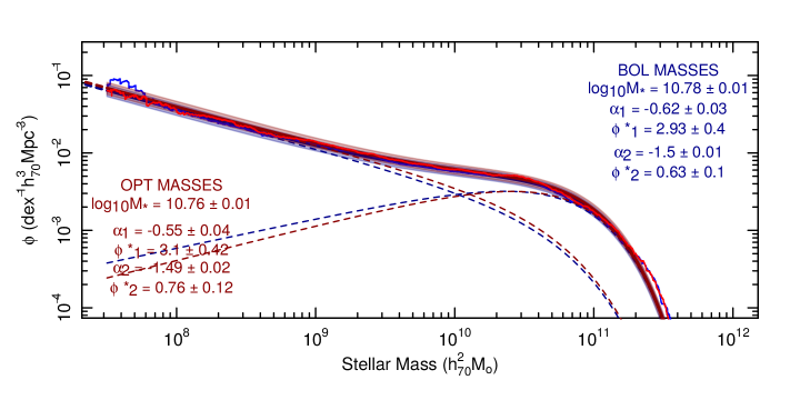
Figure 3: The galaxy stellar mass function fits as estimated using our two mass samples. The mass function using bolometric magphys stellar masses is shown in blue, and using our optical masses is shown in red. Figures are annotated with the fit parameters and uncertainties, without inclusion of systematic uncertainties;  i.e. these fits show only random uncertainties due to fitting and cosmic variance (as determined using the estimator from Driver & Robotham (2010)). Our standard systematic uncertainties on ${\mathcal{M}}^{\star}$ and $\alpha$ are not shown.

Dataset	${\mathcal{M}}^{\star}$	$\alpha_{1}$	$\phi^{\star}_{1}$	$\alpha_{2}$	$\phi^{\star}_{2}$
	$\left[\log_{10}(M_{\odot})\right]$		$(\times 10^{-3})$		$(\times 10^{-3})$
Bolometric	$\mathbf{10.78\pm 0.01\pm 0.20}$	$\mathbf{-0.62\pm 0.03\pm 0.15}$	$\mathbf{2.93\pm 0.40}$	$\mathbf{-1.50\pm 0.01\pm 0.15}$	$\mathbf{0.63\pm 0.10}$
Optical	$10.76\pm 0.01\pm 0.20$	$-0.55\pm 0.04\pm 0.15$	$3.10\pm 0.42$	$-1.49\pm 0.02\pm 0.15$	$0.75\pm 0.12$
Peng et al. (2010)	$10.67\pm 0.01\pm 0.2$	$-0.52\pm 0.04\pm 0.15$	$4.03\pm 0.12$	$-1.56\pm 0.12\pm 0.15$	$0.66\pm 0.09$
Baldry et al. (2012)	$10.66\pm 0.05\pm 0.2$	$-0.35\pm 0.18\pm 0.15$	$3.96\pm 0.34$	$-1.47\pm 0.05\pm 0.15$	$0.79\pm 0.23$
Weigel et al. (2016)	$10.79\pm 0.01\pm 0.2$	$-0.79\pm 0.04\pm 0.15$	$3.35\pm 2.31$	$-1.69\pm 0.05\pm 0.15$	$0.17\pm 0.01$
Eckert et al. (2016)	$10.87^{+0.33}_{-0.27}\pm 0.2$	$-0.52^{+0.87}_{-0.49}\pm 0.15$	$9.00^{+6.36}_{-8.47}$	$-1.38^{+0.13}_{-0.35}\pm 0.15$	$3.25^{+3.00}_{-2.81}$

Table 2: Best fit parameters of the double Schechter function for our two data sets and fitting methods, when using density-corrected maximum-volume weights. As a guide, we also show the double Schechter function fits from Peng et al. (2010), Baldry et al. (2012), Weigel et al. (2016), and Eckert et al. (2016). Our best-fit Schechter function parameters are shown in bold. Note these fits show both random uncertainties due to fitting and cosmic variance (as determined using the estimator from Driver & Robotham (2010)), and our standard systematic uncertainties on ${\mathcal{M}}^{\star}$ and $\alpha$ due to uncertainty in SPS modelling.

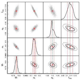
Figure 4: The posterior samples from our MCMC optimisation of the GSMF using bolometrically estimated stellar masses. Upper triangle: the individual stationary samples (grey points), and the mean of these samples (red cross). Lower triangle: the contours containing 50, 75, and 90 percent of the posterior samples (dashed, solid, and dotted lines respectively). Diagonal: marginalised PDFs of the posterior samples and their mean (red dashed line) and standard deviation (red dotted lines).

4 The Volume-Corrected Bivariate Brightness Distribution

The DCMV weighting method for estimating the GSMF, as stated in Section 3, incorporates observability corrections based solely on absolute magnitude. However, we know that there are additional selection effects within the GAMA sample, specifically around source surface-brightness and compactness. For example, due to the source definition using SDSS r-band imaging, sources that have apparent r-band surface brightnesses (averaged within $R_{e}$) lower that 23 mag arcsec^-2 will suffer incompleteness in our sample at the $30\%$ level, and at the $75\%$ level below $24.5$ mag arcsec^-2 (Blanton et al., 2005; Baldry et al., 2012; Cross et al., 2001). In order to investigate these additional known (and unknown) selection effects into our estimate of the GSMF, we can derive empirical weights from the data itself and examine the impact this has on the GSMF.

By plotting the bivariate brightness distribution (BBD) of stellar mass $M_{\star}$ and absolute average surface brightness within the effective radius $\langle\mu_{e}\rangle_{\rm abs}$, we are able to visualise the majority of the selection boundaries present in the GAMA data. Panel (a) of Figure 5 shows the observed bivariate brightness distribution for our sample of bolometric stellar masses, with lines overlaid that mark the selection boundaries of the sample (see Driver 1999). These boundaries are a mixture of observational unavoidable and intentionally imposed, owing both to the limitations of the data being analysed and the design of the GAMA survey. However, as these selection boundaries are typically defined using apparent flux and apparent size (or variations thereof), the boundaries shown in the absolute $M-\langle\mu_{e}\rangle_{\rm abs}$ plane are not sharp; rather they are blurred systematically as a function of mass-to-light ratio and redshift. We show the boundaries that would be measured at two characteristic mass-to-light ratios: $M/L=\{1,3\}$. These mark the $\sim 90^{\rm th}$ percentile limiting $M/L$ values for the GAMA low-z sample. From these boundaries we can infer the point of impact of incompleteness on our sample in $M_{\star}$-$\langle\mu_{e}\rangle_{\rm abs}$ space, and therefore estimate where our analysis becomes biased. We do this by examining which selection boundaries intersect with high-density areas of the BBD. Note also that, while panel (a) suggests that our incompleteness is most prominent at the spectroscopic and surface-brightness boundaries, to make an accurate inference we should compare each boundary to the number-density version of the BBD ( i.e. panel ‘c’), rather than the raw-count version, so that we can see if the post-correction number density is being impinged upon.

In previous studies of the GSMF, estimating surface brightness incompleteness has sometimes been achieved through simulations. For example, Blanton et al. (2005) do this by assuming a simple Gaussian analytic form for the surface brightness distribution of galaxies, and injecting galaxies sampled from this distribution into their imaging, for extraction and analysis. This allows an estimation of the fraction of successfully extracted galaxies (as a function of surface brightness), and thus an incompleteness estimate, to be made. However, inspection of the measured surface brightness distribution of galaxies shows this distribution to be somewhat more complex than a simple Gaussian distribution would suggest and that, indeed, the uncertainty on the true surface brightness distribution means that performing such an analytic estimate is likely to be biased itself.

Therefore, to estimate our surface-brightness incompleteness, we take a more pragmatic and empirical approach. We start by deriving an average weight per bin for each cell in the BBD. Within each bin we determine the weighted median redshift, where the weights are those determined by our density sampling. We then determine the volume visible to each bin and then divide the summed density-corrected weights by twice the median volume. By defining weights in this way, we assume that all selection effects bias our sample to lower redshift (rather than,  e.g. cause a net decrease in number-counts across the entire redshift range) and effectively test the assumption that, in bins of both stellar mass and surface brightness, the distribution of an unbiased sample of galaxies will have a $V/V_{\rm max}$ distribution that is uniform over $[0,1]$. If this assumption is correct, then calculating the value of binned $V_{\rm max}$ in this way should allow us to account for all systematic effects in the data, known or otherwise, without having to explicitly define them. In this way our BBD is somewhat different from a conventionally estimated BBD, such as that presented in Driver et al. (2005). We then use these weights to calculate the binned number density BBD, and can subsequently collapse this 2D distribution along the surface brightness axis to recover the binned stellar mass function. Naturally this is not as statistically elegant as our first method (in data analysis, not binning is always preferable to binning), however the exercise is useful in determining if subtle, hidden selection effects have a substantial impact on the GSMF (compared to just performing the absolute magnitude based weighting outlined in Section 3).

Panel (b) of Figure 5 shows the weights derived for each bin, and panel (c) shows the final corrected BBD for the sample. Firstly, we note that the distribution of weights is not curved or diagonal, but rather exhibits a fairly linear increase in weight solely as a function of stellar mass. This suggests that our sample is not strongly sensitive to surface-brightness effects, even down to our spectroscopic completeness selection limit. Indeed, examination of the distribution of $V/V_{\rm max}$ values in bins of stellar mass shows a strong evolution, whereas in bins of surface brightness only a minor change seen. Secondly, the number-density distribution in panel (c) appears to be reasonably well bounded by the two diagonal selection boundaries, as the number density is declining well before these limits. This suggests that there is not a substantial population of massive low surface brightness galaxies, nor highly compact galaxies, that we have missed because of selection effects. Naturally this does not exclude that these galaxies can exist (indeed, rare examples of extremely massive low surface brightness galaxies have been known to exist for decades; see Bothun et al. 1987) but rather suggests that they do not contribute greatly to the number-density of galaxies (Cross et al., 2001; Driver, 1999; Davies et al., 2016). Finally, panel (d) of Figure 5 shows the binned-GSMF measured from the BBD using our bolometric masses. This is shown jointly with our DCMV GSMF, as a demonstration of the agreement between these analysis methods in the $M_{\star}>10^{8}M_{\odot}$ regime. There is a slight indication of a possible excess in the BBD GSMF at masses below $10^{8}M_{\odot}$, suggesting that incompleteness may likely be affecting our sample below this point.

Panels (e)-(h) of Figure 5 show the same as (a)-(d), but for our optical-based sample of stellar masses. For this sample we can see the same trends as for the bolometric mass sample, and similarly good agreement between the two GSMFs for this sample.

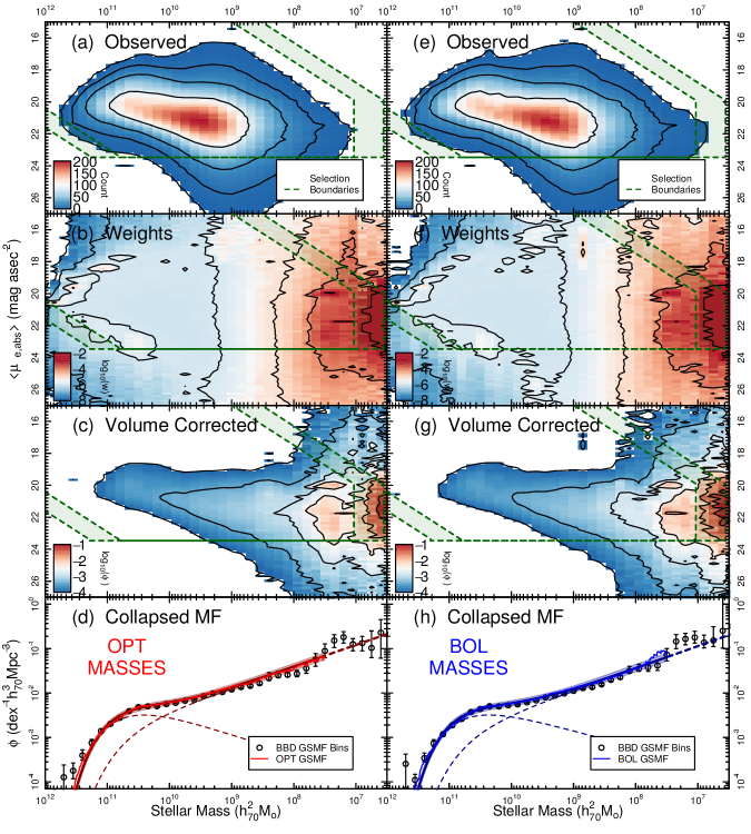
Figure 5: The galaxy bivariate brightness distribution space, averaged over MC iterations, as a function of raw counts (panels a+e), density-corrected weight per bin (panels b+f), and number density (panels c+g). Panels d+h show the binned GSMF determined by collapsing panels c+g onto their respective x-axis. Overplotted in these panels is the DCMV GSMF for the same sample, demonstrating agreement between the mass functions returned using these methods. Note that the binned GSMFs in panels c+d do not include the additional cosmic variance uncertainty in their error bars.

4.1 Extension to Future Surveys

We have derived four estimates of the GSMF for the full GAMA $0.002<z<0.1$ sample, summarised in Table 2. We find GSMFs that are in agreement with previous GAMA estimates, for fits to a limiting mass of $10^{7.5}M_{\odot}$. However, there is a suggestion that we may be incomplete below $10^{8}M_{\odot}$, where we become restricted in our fitting power by the surface-brightness limit of SDSS imaging (which was used to select the GAMA sample).

Our estimates of the GSMF are predominantly limited by the selection boundaries in spectroscopic completeness and surface brightness. Figures 5 and 6 demonstrate these selection boundaries, as well as other boundaries that affect our analysis to a lesser degree (namely compactness, sparseness, and rarity). Despite these limits, however, we are able to construct a GSMF that is representative down to masses as low as $\sim 10^{6}M_{\odot}$, by simply continuing our empirical reconstruction beyond $10^{7.5}M_{\odot}$, as we will show in Section 4.2. There is evidence of a systematic incompleteness bias below $10^{8}M_{\odot}$, which confirms our concerns regarding incompleteness, but nonetheless the mass function shows continuity consistent with the extrapolation below this limit ( i.e. the impact is subtle, not severe).

Because of the incompleteness effects in GAMA, it is desirable to extend this work using future deep large-area surveys if we wish to constrain the GSMF to yet lower masses using a single sample. To demonstrate this, Figure 6 shows the selection boundaries for two future surveys: the Wide Area Vista Extragalactic Survey (WAVES; Driver et al. 2016b), and the galaxy evolution survey on the Mauna Kea Spectroscopic Explorer (MSE; McConnachie et al. 2016). WAVES and MSE will both utilise imaging that is substantially deeper than the GAMA SDSS imaging, and will have high-completeness spectroscopic campaigns that push many magnitudes fainter than was possible for GAMA. As a result, these surveys will both substantially expand the available parameter space available to be studied for galaxy evolution, as can be seen by the expansion of the limits in Figure 6. As a demonstration, we include galaxies measured in the local-sphere in this figure, to indicate where it is expected that the majority of galaxies might lie in this plane (beyond the limits of GAMA). For these points, we have used the local sphere catalogue from Karachentsev et al. (2004) and the “maintained” local group sample from McConnachie (2012). Finally, we include the selection-boundaries of a low-surface brightness survey using the Dragonfly telephoto array (Abraham & van Dokkum, 2014), which clearly opens up a very different part of the parameter space.

The samples of Karachentsev et al. (2004) and McConnachie (2012) are particularly useful in inferring the likely incompleteness of our sample. In particular, it is telling that half of the McConnachie (2012) sample with mass greater than $10^{7.5}M_{\odot}$ lies below our nominal surface brightness completeness limit. This provides further suggestion that our sample is likely incomplete below this level. It is clear that the next generation of wide-area spectroscopic surveys, such as WAVES-wide, will be paramount in determining the shape of the low-mass tail of the stellar mass function. Prior to the execution of these large surveys, however, we can perform a similar analysis by combining the wide-area power of GAMA with a more directed, deeper survey, such as the G10-COSMOS.

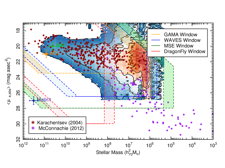
Figure 6: The bivariate-brightness distribution for the GAMA $z<0.1$ sample. We overlay the selection boundaries for GAMA, as well as the expected limits for three future surveys: the WAVES-Wide survey on 4-MOST, a similar-time survey on MSE, and the Dragonfly LSB survey. Furthermore, we overplot data from the local sphere and local group as a demonstration of where as-yet-undetected galaxies beyond the local sphere are expected to lie, as well as some individual galaxies of note: Milky Way (green dot), Andromeda (orange dot), and Malin 1 (blue dot).

Table 3: Survey parameters of GAMA, G10-COSMOS, and 3 additional surveys

Survey	Area	Selected	Spec. Limit	Surf. Brightness	Resolution	Pixel Width	Completeness
	(deg2)	From	(mag)	Lim. (mag/arcsec2)	(′′)	(′′)	($\%$ within limit)
GAMA	180	SDSS	19.8	24.5	1.2	0.339	$>98$
G10-COSMOS	1	HST	24.5	24.5	1.2	0.339	$\sim 40$
DragonFly	180	SDSS	19.8	30.5	5.5	2.3	$>98$
WAVES-Wide	1500	VST KiDS	22	26.5	0.6	0.2	$>95$
MSE	12000	LSST	24	28	0.6	0.2	$>95$

4.2 Exploiting GAMA + G10-COSMOS

While we will require surveys like WAVES and MSE in order to constrain the GSMF in a robust fashion below $10^{7.5}M_{\odot}$ using a single dataset, we note that by splicing our GAMA equatorial sample with the G10-COSMOS sample of Andrews et. al. (2016), we can generate an indication of how the GSMF behaves to masses lower than $10^{7.5}M_{\odot}$. For the G10-COSMOS dataset, we use lambdar photometric measurements of approximately 170,000 galaxies compiled by Andrews et. al. (2016), along with a combination of spectroscopic and photometric redshifts from Davies et al. (2015a), taken predominantly from Laigle et al. (2016), and fit these galaxies with magphys (as we did with the GAMA equatorial sample, see Driver et. al. 2016a). The coverage in the G10 field of 1sqdeg is not nearly as high as in the equatorial GAMA fields, but the sample extends $\sim 5$ mag fainter in the r-band.

Using this combined sample, we are able to construct an indicative GSMF to much lower masses than can be probed by GAMA alone. We construct a simple binned GSMF for the G10 sample, without any attempt to match samples or normalisation to those in GAMA. This combined dataset is shown in Figure 7. Data for the binned GAMA GSMF shown in the figure is provided as a machine readable file alongside this work.

We see general agreement between the extrapolated best-fit GAMA GSMF and the G10-COSMOS sample down to masses as low as $10^{6}M_{\odot}$, with the exception of a modest bump in the faint end slope seen around $10^{7}M_{\odot}$. This bump is likely to arise from Eddington bias induced by the large stellar mass uncertainties, however the similar rise in the low mass tail of the GAMA BBD is a tantalising suggestion of, perhaps, a slight rise in the faint end slope of the mass function. Nonetheless, this function rejoins our extrapolation at $10^{6}M_{\odot}$, nominally below where we expect incompleteness to be problematic in the COSMOS field, and so we conclude that (for now) there appears to be no sign of any major up- or down-turn to this limit.

Naturally this comparison is a qualitative rather than quantitative measure. Nonetheless the agreement between the datasets in the range of overlap is good, and overall provides a glimpse into the very low mass population and that extrapolation to $10^{6}M_{\odot}$ is not unreasonable.

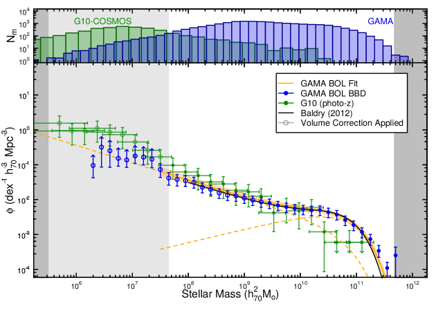
Figure 7: The GSMF measured when combining data from GAMA with that from G10-COSMOS. Uncertainty in the Mass direction for the G10-COSMOS binned data indicate the median uncertainty in that bin caused only by photometric redshift uncertainties. For this, we assume a standard $\Delta z_{p}=0.02$. From these uncertainties we can see that ‘bump’ in number density coincides with where Eddington bias becomes considerable, given the photometric redshift uncertainties. The inclusion of the G10-COSMOS allows us to probe to $10^{7.7}M_{\odot}$ without requiring any $V_{\rm max}$ corrections, and when incorporating corrections we are able to extend to masses as low as $10^{6}M_{\odot}$. Note, however, that we show bins requiring volume corrections with open circles, to indicate that these bins may be biased by poorly determined redshift estimates, particularly in the G10-COSMOS. Note also that the G10-COSMOS GSMF includes uncertainty due to cosmic variance using the estimator from Driver & Robotham (2010). The light and dark grey regions in the figure indicate the masses where we believe GAMA is systematically incomplete, and where both samples have low number statistics, respectively.

5 Contribution to $\Omega_{\star}$

To conclude, we can utilise our fitted GSMF to derive the value of the stellar mass density parameter $\Omega_{\star}$ and the fractional contribution of stars to the universal baryon density $\Omega_{b}$. Furthermore, we can be somewhat confident in extrapolating our fit down to much lower masses than GAMA alone would allow, given the consistency we see in the GAMA+G10-COSMOS GSMF. Figure 8 shows the distributions of stellar mass number density $\phi$, and mass density $\rho$, for our final GSMF. In the figure we also compare these distributions to those from the GALFORM semi-analytic models of Lacey et al. (2016); Gonzalez-Perez et al. (2014), and to the hydrodynamic simulations from EAGLE Schaye et al. (2015); Crain et al. (2015).

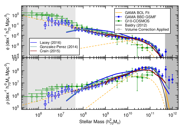
Figure 8: Our measured stellar mass function, shown as number density and mass density, compared to those measured in GALFORM semi-analytic models and EAGLE hydrodynamic simulations. The bin uncertainties in the mass-direction show the median mass uncertainty for sources in that bin which are caused only from (an assumed typical) standard photometric redshift uncertainty $\Delta z_{p}=0.02$. Note that the G10-COSMOS binned GSMF, and the GAMA DCMV GSMF fit, both include their respective uncertainties due to cosmic variance using the estimator from Driver & Robotham (2010) in the number density direction. The light and dark grey regions in the figure indicate the masses where we believe GAMA is systematically incomplete, and where both samples have low number statistics, respectively.

From the mass density distribution in Figure 8, we can see that the stellar mass density is dominated by ${\mathcal{M}}^{\star}$ galaxies, as has long been known. Our distributions match exceptionally well with the simulations, although this is somewhat by design given that the GALFORM semi-analytic models are calibrated to the B_j- and K-band luminosity functions at $z=0$ (Lacey et al., 2016; Gonzalez-Perez et al., 2014). We find a final $\Omega_{\star}=1.66^{+0.24}_{-0.23}\pm 0.97h^{-1}_{70}\times 10^{-3}$, corresponding to an overall percentage of baryons stored in bound stellar material $f_{b}=6.99^{+1.01}_{-0.97}\pm 4.09$ (assuming the Planck $\Omega_{b}=23.76\times 10^{-3}h^{-2}_{70}$), inclusive of uncertainty due to cosmic variance and systematic uncertainties in SPS modelling.

With respect to random uncertainties only, our estimate represents the most stringent constraint on the bound component of both $\Omega_{\star}$ and $f_{b}$ to date. As expected, however, our estimates of both $\Omega_{\star}$ and $f_{b}$ are overwhelmingly dominated by the systematic uncertainties in our mass estimation. Nonetheless, as these systematic uncertainties are inherently present in all estimates of stellar masses, we can still perform an informative comparison between our value of $\Omega_{\star}$ and a sample from the literature (seen in Figure 9). This distribution shows that, since 2008 there has been a reasonable consensus regarding the estimates of $\Omega_{\star}$. This consensus is due, at least in part, by a consistent use of Bruzual & Charlot (2003) SPS models in each of the post-2008 estimates (with the exception of that from Moustakas et al. 2013, who use a similar but nonetheless different Conroy & Gunn 2010 model), and to an increase in sample sizes with the advent of big-data astronomy. In any case, the fact that all of these estimates are subject to the same systematic uncertainties indicates that, as a community, we are unlikely to gain further significant insight into the amount of mass stored in bound stellar systems without: a significant reduction in the systematic uncertainties of stellar mass estimates, a significant reduction in the masses of systems that we can analyse (see Section 4.1), or both.

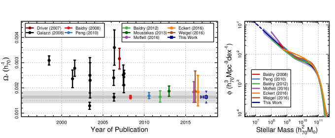
Figure 9: Left: Contribution of the full GAMA sample to $\Omega_{\star}$, compared to previous estimates from the literature. The two blue data points from this work correspond to estimates incorporating only the formal uncertainty on the fit (solid symbol, dark grey shaded bar), and that including uncertainty due to cosmic variance (open symbol, light grey shaded bar). Note the fit uncertainty is smaller than the data point in the former case, and therefore has been shown as a white bar within the data point. No data displayed here includes systematic uncertainty due to stellar mass modelling and, with the exception of our open symbol data point, no measurement uncertainties displayed here include uncertainty due to cosmic variance. Right: the GSMFs corresponding to the most recent estimates of $\Omega_{\star}$ in the left panel. This provides an indication of the level of concordance in the literature with regards to the overall shape of the GSMF, and also of the level of variation in the GSMF required to create a significant change in the value of $\Omega_{\star}$.

6 Conclusions

We present the revised galaxy stellar mass function for the GAMA $z\leq 0.1$ sample, expanding on the GAMA-I analysis presented in Baldry et al. (2012) to the full GAMA-II dataset in this volume. We utilise two stellar mass samples, calculated with and without consideration for the impact of optically thick dust, finding no discernible difference between these samples. As in Baldry et al. (2012), we calculate the GSMF using density-corrected maximum-volume (DCMV) weights, defining our fiducial density using galaxies with $M_{\star}\geq 10^{10}M_{\odot}$ in the redshift range $0.07<z<0.19$. Within these limits the cosmic structure is fairly uniform, the sample is not yet affected by incompleteness, and the volume is influenced by cosmic variance at the $<10\%$ level (using the cosmic variance estimator from Driver & Robotham 2010), allowing for a stable constraint on the fiducial average density. We fit the GSMF using a Markov-Chain Monte-Carlo and mass limits defined in a manner that is conservative with respect to incompleteness in both brightness and colour. We choose to fit the GAMA low-z GSMF with a double Schechter (1976) function, finding best fit parameters $\mathcal{M}^{\star}=10^{10.78\pm 0.01\pm 0.20}M_{\odot}$, $\phi^{\star}_{1}=(2.93\pm 0.40)\times 10^{-3}h_{70}^{3}$Mpc^-3, $\alpha_{1}=-0.62\pm 0.03\pm 0.15$, $\phi^{\star}_{2}=(0.63\pm 0.10)\times 10^{-3}h_{70}^{3}$Mpc^-3, and $\alpha_{2}=-1.50\pm 0.01\pm 0.15$, where the second uncertainty components on $\mathcal{M}^{\star}$ and each $\alpha$ encode the systematic uncertainty on stellar mass estimation due to SPS modelling uncertainties. The uncertainty due to cosmic variance is included in the stated uncertainties on $\phi^{\star}_{1}$ and $\phi^{\star}_{2}$. While the value of ${\mathcal{M}}^{\star}$ here is higher than other works in the literature, we argue that this is a result of the dedicated by-hand effort that was undertaken to ensure photometry of the brightest systems in GAMA was accurately determined (Wright et al., 2016).

We explore the galaxy bivariate brightness distribution of stellar mass and absolute surface brightness in order to explore the possible surface brightness incompleteness of our dataset. Our BBD GSMFs both agree well with our nominal best-fit GSMFs from above, however there is a slight excess in both mass samples at the lowest stellar masses. Furthermore, the location of the known GAMA selection boundaries, and the distributions of known local sphere galaxies from Karachentsev et al. (2004) and McConnachie (2012), both suggest that our sample may be incomplete below $10^{8}$ in stellar mass.

To further explore the low-mass end of the GSMF, we compare our estimated stellar mass function to the GSMF measured using the same analysis applied to the G10-COSMOS dataset Davies et al. (2015b); Driver et. al. (2016a); Andrews et. al. (2016). We find good agreement between the stellar mass functions, and an indication that the faint end slope of the GSMF is relatively well behaved down to masses as low as $M>10^{6}M_{\odot}$, showing an only marginal feature at $\sim 10^{7}M_{\odot}$.

We compare our measured mass function to those from the GALFORM semi-analytic models (Lacey et al., 2016; Gonzalez-Perez et al., 2014), and to the GSMF from the EAGLE hydrodynamic simulation (Schaye et al., 2015; Crain et al., 2015). We find an exceptional agreement between the GALFORM semi-analytic models and our GSMF, however this is arguably somewhat by design as the semi-analytic models are calibrated to the B_j- and K-band luminosity functions at $z=0$ (Lacey et al., 2016; Gonzalez-Perez et al., 2014).

We compute the value of the stellar mass density parameter $\Omega_{\star}$ for our mass function fit, finding $\Omega_{\star}=1.66^{+0.24}_{-0.23}\pm 0.97h^{-1}_{70}\times 10^{-3}$, corresponding to an overall percentage of baryons stored in bound stellar material $f_{b}=6.99^{+1.01}_{-0.97}\pm 4.07$ (assuming the Planck $\Omega_{b}=23.76\times 10^{-3}h^{-2}_{70}$), inclusive of uncertainty due to cosmic variance and systematic uncertainties from SPS modelling. Finally, using the joint dataset from GAMA and G10-COSMOS, we conclude that there is no strong indication of a significant up- or down-turn in the GSMF to stellar masses greater than $10^{6}M_{\odot}$. We conclude that the integrated stellar mass density of bound material down to $M>10^{6}M_{\odot}$ is well constrained, and that the fraction of universal baryonic matter stored in bound stellar material within galaxies (assuming our various SPS model parameters) is unlikely to exceed $\sim 8\%$. However, systematic uncertainties from the SPS models dominate our error-budget, and could possibly drive this value as high as $\sim 20\%$, assuming the most extreme SPS and IMF models. Additionally, the question of the amount of unbound stellar mass in halos remains open.

Appendix A Fits without Fluxscale Correction

As discussed in Section 3 the fluxscale parameter, while necessary, may be affected by unrecognised systematic biases. Here we present the GSMF and $\Omega_{\star}$ estimates determined when not incorporating the fluxscale parameter. This provides a quasi-lower limit on our fits and parameter estimations, and demonstrates the impact of this corrective factor.

Figure 10 shows the final GSMF estimated when not incorporating the fluxscale parameter. It is the no-fluxscale equivalent of Figure 3. Similarly, Figure 11 shows the final estimate of $\Omega_{\star}$ when not incorporating the fluxscale parameter.

In these figures, we can see that the most substantial change is in the extent of the GSMF to the highest masses. This is not surprising as the fluxscale factor is expected to influence high Sersic index sources the most, and these are overly contained at the highest mass end of the sample ( e.g. elliptical sources and bulge-dominated disks). The result is that our sample loses a substantial amount of mass in the same region where the mass-density function peaks. This drives the significant loss in the stellar mass density parameter.

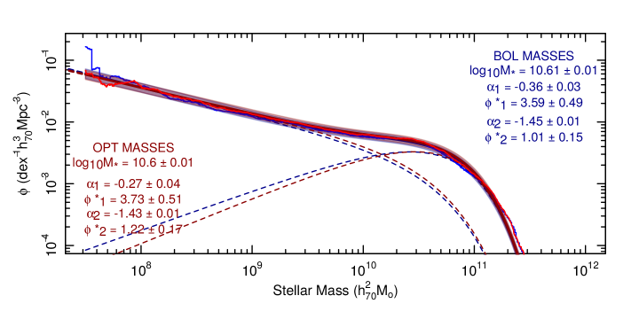
Figure 10: The best-estimate GSMF for the GAMA low-z sample when not performing the fluxscale correction. The figure annotations are the same as in Figure 3. Note that these fits include uncertainty due to cosmic variance using the estimator from Driver & Robotham (2010). Our standard systematic uncertainties on ${\mathcal{M}}^{\star}$ and $\alpha$ are not shown.

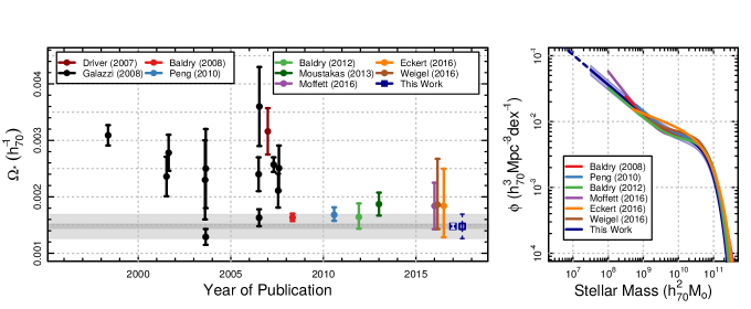
Figure 11: Left: Contribution of the full GAMA sample to $\Omega_{\star}$, compared to previous estimates from the literature, when not incorporating the fluxscale correction. The figure is annotated as in Figure 9. Right: the GSMFs corresponding to the most recent estimates of $\Omega_{\star}$ in the left panel. This provides an indication of the level of concordance in the literature with regards to the overall shape of the GSMF, and also of the level of variation in the GSMF required to create a significant change in the value of $\Omega_{\star}$.

Appendix B Fits with decoupled ${\mathcal{M}}^{\star}$

As discussed in Section 4, we opt to fit our main GSMFs with a coupled ${\mathcal{M}}^{\star}$ 2-component Schecter function. This choice is motivated mostly to enable simple comparison with previous GSMF fits. However extensive work in exploring individual populations of galaxies separated by morphology and dynamical properties (Moffett et al., 2016; Kelvin et al., 2014), demonstrate that many decoupled Schechter functions are required to capture the true diversity of galaxy mass functions. With this in mind, we briefly explore the fits obtained when using a decoupled 2-component Schechter function, in Figure 12.

The fit parameters from our decoupled fit indicate that data prefers a decoupled ${\mathcal{M}}^{\star}$ only slightly. The two free ${\mathcal{M}}^{\star}$ parameters end up with values that are only slightly inconsistent with each other, and otherwise the fit parameters are largely unchanged from our original coupled fits. Nonetheless, the fact that the lower-mass component favours a slightly lower ${\mathcal{M}}^{\star}$ than the higher mass component is consistent with the results found previously in the literature, such as previously in the GAMA low-z sample by Moffett et al. (2016).

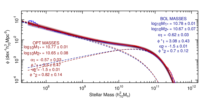
Figure 12: The best-estimate GSMF for the GAMA low-z sample when fitting with decoupled ${\mathcal{M}}^{\star}$ parameters. The figure annotations are the same as in Figure 3. Note that these fits include uncertainty due to cosmic variance using the estimator from Driver & Robotham (2010). Our standard systematic uncertainties on ${\mathcal{M}}^{\star}$ and $\alpha$ are not shown.

Appendix C Deriving Mass Limits

For the automated derivation of mass limits, we fit a polynomial to bootstrapped estimates of the turn-over point of the comoving galaxy number density as a function of stellar mass, and of the turn over of the stellar mass density as a function of comoving distance. The result of this procedure is shown in Figure 13, where we show the individually estimated turn-over points in each dimension. These points have then been fit by a polynomial, yielding the mass limit function shown. Importantly, Figure 14 demonstrates that the mass limits successfully debias the sample with respect to colour, as seen by the mass limit preferentially removing blue galaxies (which are visible to higher redshifts than their red counterparts).

We then determine the fidelity of these mass limits by comparing the distribution of the mass-limited galaxy probability function (with redshift) when using these mass limits and the mass limits implemented in Moffett et al. (2016). To do this, we assume a Baldry et al. (2012) double Schechter function and compute the probability of observing each galaxy given this GSMF and the assigned mass limit. The distribution of probabilities using these two mass limit functions are given in Figure 15. These figures show the distribution of galaxy probabilities assuming a Baldry et al. (2012) generative distribution and the relevant mass-limit function. If both of these are a good reflection of the data, the distribution of probabilities should have an expectation of $0.5$. In these figures we can see that the Moffett et al. (2016) mass limits are systematically biased at low redshift, indicated by an expectation systematically different from $0.5$. Conversely, we see that the automatically defined mass limits show no such systematic bias.

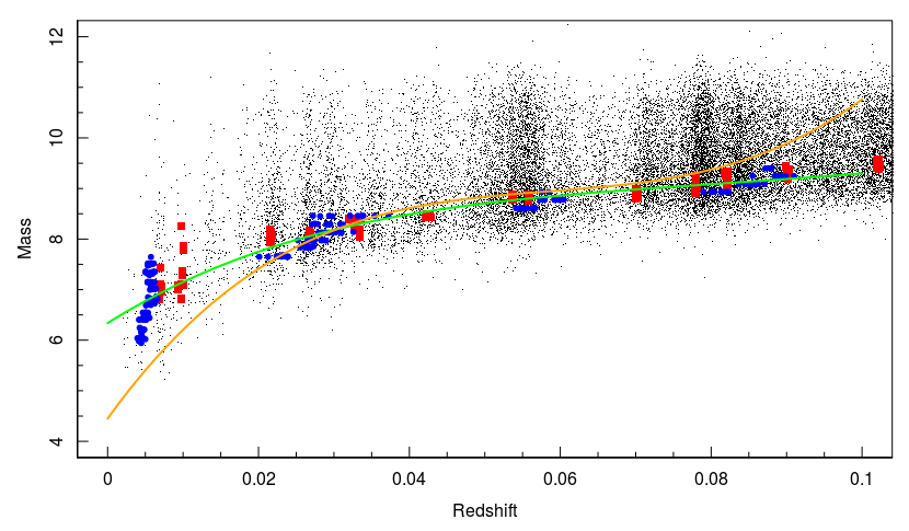
Figure 13: Demonstration of the stellar mass limits returned by our automated mass limit estimation procedure. Here we can see the distribution of bootstrapped turn-over estimates, derived in comoving distance bins (red) and mass bins (blue). These turn over estimates are then fit with a polynomial (green). For comparison, the mass limit function of Moffett et al. (2016) is shown in orange. Note that this is a generic diagnostic figure output by the function, and therefore is intentionally not created with meaningful axis labels.

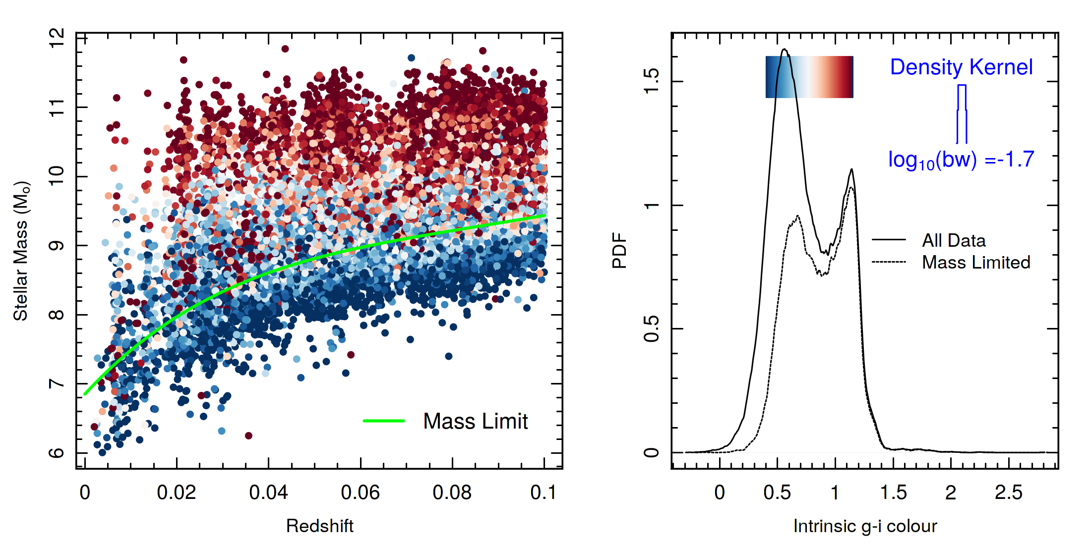
Figure 14: Demonstration that the stellar mass limits returned by our automated mass limit estimation procedure adequately debias the colour distribution of galaxies within our sample. The left-hand figure shows the mass-redshift space of all galaxies within our sample, coloured by g-i colour, along with the mass limit function. The distribution of colours (and the colour-bar) is shown in the right hand panel. The solid line in the right hand figure is the colour distribution of the full sample, and the dashed line shows the distribution after applying the mass-limit cut. Note in-particular that the mass-limit cut preferentially removes blue galaxies, which are visible to higher redshifts (at a given stellar mass) than their red counterparts.

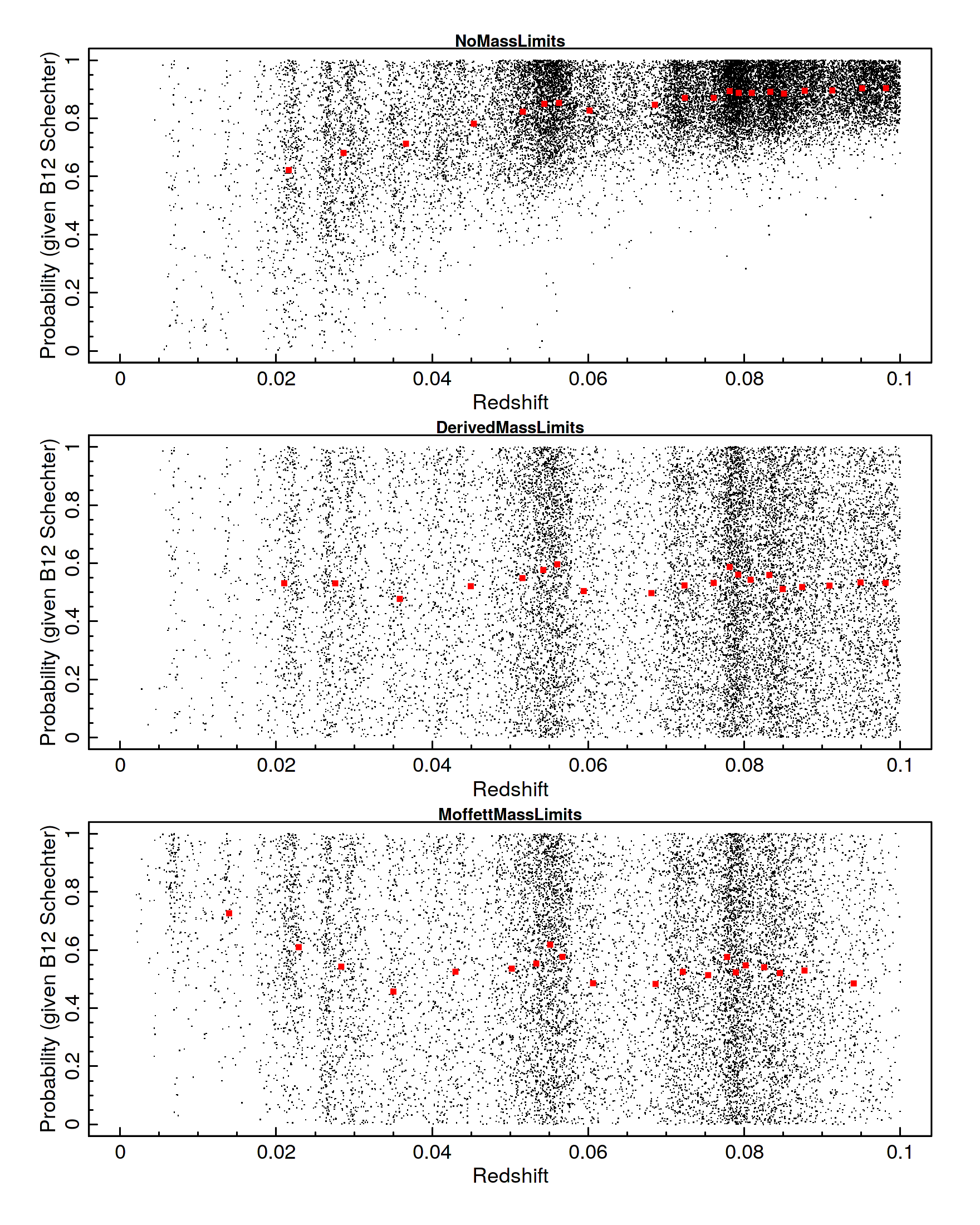
Figure 15: Comparison between the galaxy probability distribution assuming: (top) constant mass limits, (middle) those derived using our automated procedure, and (bottom) mass limits presented in Moffett et al. (2016). We see that the Moffett et al. (2016) mass limits show a deviation away from the expectation probability (red points) of 0.5 at low masses, indicating that the mass limit there is not accurate (assuming, of course, that the GSMF is reasonably represented by the Baldry et al. 2012 GSMF). Conversely, the automatically defined mass limits returned from our procedure show no such bias.

References

- Abraham & van Dokkum (2014) Abraham R. G., van Dokkum P. G., 2014, PASP, 126, 55
- Andreon (2002) Andreon S., 2002, A&A, 382, 495
- Andrews et. al. (2016) Andrews et. al. 2016, accepted