Optical and X-ray luminosity of expanding nebulae around ultraluminous X-ray sources

Abstract

We have performed a set of simulations of expanding, spherically symmetric nebulae inflated by winds from accreting black holes in ultraluminous X-ray sources (ULXs). We implemented a realistic cooling function to account for free-free and bound-free cooling. For all model parameters we considered, the forward shock in the interstellar medium becomes radiative at a radius $\sim 100$ pc. The emission is primarily in the optical and UV, and the radiative luminosity is about 50% of the total kinetic luminosity of the wind. In contrast, the reverse shock in the wind is adiabatic so long as the terminal outflow velocity of the wind $v_{\rm w}\gtrsim 0.003c$. The shocked wind in these models radiates in X-rays, but with a luminosity of only $\sim 10^{35}\,{\rm erg\,s^{-1}}$. For wind velocities $v_{\rm w}\lesssim 0.001c$, the shocked wind becomes radiative, but it is no longer hot enough to produce X-rays. Instead it emits in optical and UV, and the radiative luminosity is comparable to 100% of the wind kinetic luminosity. We suggest that measuring the optical luminosities and putting limits on the X-ray and radio emission from shock-ionized ULX bubbles may help in estimating the mass outflow rate of the central accretion disk and the velocity of the outflow.

1 Introduction

Ultraluminous X-ray sources (ULXs; see Feng & Soria 2011 for a recent review) are the most luminous persistent point X-ray sources located outside the nuclei of galaxies. Although some may host intermediate-mass black holes with masses $\sim 10^{2}-10^{5}~{}M_{\odot}$ (Farrell et al., 2009; Davis et al., 2011; Mezcua et al., 2015), the majority are now thought to be less massive compact objects that accrete at extreme rates (e.g. Gladstone et al. 2009; Sutton et al. 2013; Liu et al. 2013; Motch et al. 2014), with at least 3 objects now confirmed to be neutron stars on the basis of displaying X-ray pulsations (Bachetti et al., 2014; Israel et al., 2016; Fürst et al., 2016).

Optical observations of ULXs reveal bubble-like nebulae (henceforth ULX bubbles — ULXBs), with diameters of up to 500 pc (e.g. Pakull & Mirioni 2002; Roberts et al. 2003; Ramsey et al. 2006; Abolmasov et al. 2007; Moon et al. 2011; Cseh et al. 2012). Based on standard diagnostic optical line ratios (e.g., [S II]/H$\alpha$, [N II]/H$\alpha$, [O III]/H$\beta$), it was determined (Pakull & Mirioni, 2002; Pakull et al., 2005a; Moon et al., 2011) that some of these nebulae contain mostly X-ray photo-ionized gas, while others result mostly from shock-ionization. X-ray photoionized nebulae such as those around the ULXs in Holmberg II (Kaaret et al., 2004; Pakull & Mirioni, 2002) and NGC 5408 (Kaaret & Corbel, 2009) constrain the isotropic photon luminosity and collimation angle of the compact source. Shock-ionized ULXBs expand into the interstellar medium (ISM) at a speed of a few 100 km s^-1 over characteristic timescales of up to $10^{6}$ yr (Pakull et al., 2005a). In this paper, we focus specifically on shock-ionized ULXBs: we model their physical structure and luminosity at different evolutionary stages.

The mechanical power required to inflate a ULXB can be estimated from optical observations in two independent ways (Pakull et al., 2010): either from the flux emitted in specific diagnostic lines (e.g., H$\beta$ and [Fe II] $\lambda$1.64$\mu$m), or from their size and expansion speed (with plausible assumptions on the ISM density). Both methods suggest that ULXBs contain at least one order of magnitude more energy than an ordinary supernova remnant, as well as being much larger and longer-lived. Several formation scenarios have been proposed.

In one scenario, the bubbles are inflated by outflows from multiple O stars and supernova remnants, forming a so-called "superbubble" An alternative scenario is that they result from "hypernova" events, which may inject a large amount of energy (up to $\sim$10⁵³ erg) in a single explosion. However, both of these formation scenarios are disfavored by observations (Pakull et al., 2005a, b). In most cases, the stellar population inside and around ULXBs is moderately old ($\approx$20 Myr), does not contain stars massive enough to produce hypernovae at the current epoch, and does not contain enough OB stars to produce superbubbles.

A more likely scenario is that ULXBs are formed by the continuous injection of winds/jets from an accretion disk surrounding a black hole or neutron star at the centre of the ULX. Interestingly, this is qualitatively consistent with the super-Eddington models that have been invoked to explain many of the X-ray characteristics of ULXs (Poutanen et al., 2007; Kawashima et al., 2012; Middleton et al., 2015; Narayan et al., 2017), where the extreme radiation release from the central regions of the super-Eddington accretion flow drives a massive wind away from the accretion disc; such a wind may be a prime culprit for the inflation of the ULXBs. In this model, the wind would need to input $\sim 10^{39}{\rm erg\,s^{-1}}$ into the nebula to inflate it, meaning the mechanical output of ULX disks must be similar to their radiative output (Pakull & Mirioni, 2002; Roberts et al., 2003). Evidence for this wind has recently emerged from X-ray observations, with the detection of absorption features from a medium that is outflowing at a velocity $\sim 0.2c$ in the high resolution X-ray spectra of two ULXs (Pinto et al., 2016). Rest-frame emission lines are also detected that might be attributable to collisional heating in the vicinity of the ULX, although, with the current quality of data, photoionization models also provide a plausible explanation for these features. Meanwhile, general relativistic radiation MHD simulations of super-Eddington black hole accretion have also confirmed that such systems invariably produce powerful winds (Sądowski et al., 2014; McKinney et al., 2014; Narayan et al., 2017).

In this paper we investigate the ULX disk wind model in detail. We perform numerical simulations of expanding nebulae with realistic cooling and track the evolution of the shocked gas. We investigate the properties of the shocked wind and the related optical and X-ray emission as a function of the disk outflow parameters. We suggest that optical and X-ray (and potentially radio) emission properties of the ULX nebulae may constrain the characteristics of the outflows blown out of the accreting systems.

The paper is structured as follows. We first describe the numerical methods and the setup of our simulations (Section 2). We then discuss the properties of the expanding nebula in the fiducial model (Section 3.1), followed by a parameter study where we investigate the effect of wind velocity on the nebular properties (Section 3.2). Caveats and astrophysical implications are discussed in Section 4, and the results are summarized in Section 5.

2 Numerical methods

2.1 KORAL

In the scenario investigated in this paper, the expanding nebulae in ULXBs result from kinetic power pumped out by a central accreting black hole (BH) via a quasi-spherical wind. The outflowing gas pushes and shocks the ISM. The nebula is optically thin, but may cool significantly enough to affect its dynamics.

The simulations described here were carried out with the code KORAL (Sądowski et al., 2013, 2014), which is capable of evolving magnetized gas and radiation in parallel in a relativistic framework, for arbitrary optical depths. In the project described here, we neglect magnetic fields, the gravity of the BH (since the interesting interaction of the outflow with the ISM takes place at large radii), and radiative transfer (since the gas is optically thin throughout the expansion). We also assume isotropic expansion of the nebula and evolve the problem in one (radial) dimension.

2.2 Cooling function

To account for bound-free and free-free cooling we provide KORAL with opacities calculated from a cooling function generated with ChiantiPy, the Python interface to the Chianti database (Dere et al., 1997; Zanna et al., 2015). Figure 1 shows the radiative loss rate we use in the present study (obtained with the Chianti RadLoss function, assuming solar abundances).

Although the cooling rate falls off naturally at temperatures of order $10^{4}$ K or below, we reduce it further to ensure that the unperturbed ISM, which is at an equilibrium temperature of $10^{4}$ K through cosmic ray heating, does not cool significantly during the course of the simulation. We leave the cooling function obtained through ChiantiPy unmodified between $10^{4}$ K and $10^{8}$ K, and then extrapolate up to $10^{11}$K assuming pure free-free emission. Including a relativistic correction (Sądowski et al., 2016), we assume the following broken power-law for the cooling function at high temperatures,

$$\frac{\Lambda_{\rm ff}\color[rgb]{0,0,0}}{n_{\rm i}n_{\rm e}}=2.409\times 10^{-27}\sqrt{T}\left(1+4.4\times 10^{-10}T\right)\ {\rm erg\,cm^{3}\,s^{-1}},\quad T>10^{8}\,{\rm K}.$$ (1)

The above opacities are used when calculating the source terms that describe energy loss of the gas due to radiation (Sądowski et al., 2013). Since the gas is optically thin, no radiative transfer calculation is done as part of the simulation.

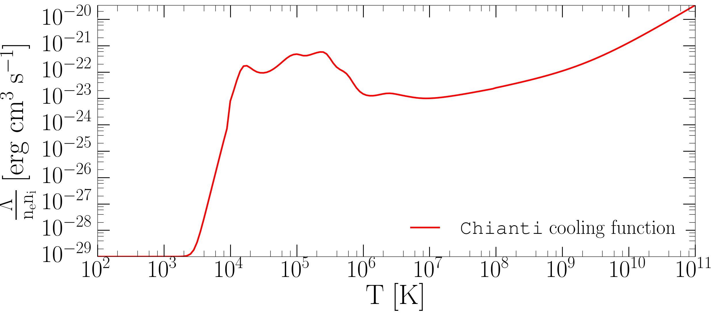
Figure 1: Gas emissivity $\Lambda$ for solar abundances as a function of temperature $T$, obtained from the CHIANTI Database Version 8. Above $T=10^{8}K$, the emissivity is modelled as a broken power-law to account for relativistic bremsstrahlung (equation 1).

2.3 Numerical setup

Current observations (Pakull et al., 2005a, b) suggest that ULXBs are formed by the continuous injection of winds/jets from the accretion disk surrounding the black hole at the centre of the ULX. The underlying physics has been extensively studied, most notably by Castor et al. (1975) and Weaver et al. (1977), in the context of interstellar bubbles formed by the interaction of stellar winds with the ISM.

The simulations are set up as follows. We introduce an isotropic wind which has been emitted from the accretion disk but has since reached some constant velocity $v_{w}$ far from the disk. This wind expands and propagates freely into the ISM until its density is equal to that of the ambient medium. The radius at which this happens is called the initial contact surface (CS) and depends on the kinetic wind luminosity $L_{w}$, wind velocity $v_{\rm w}$ and the density of the surrounding ISM $\rho_{\rm ISM}$.

For a fixed kinetic luminosity and wind velocity, the density of the wind $\rho_{w}$ varies with radius $r$ as

$${\rho_{\rm w}=\frac{L_{\rm w}}{2\pi r^{2}v_{\rm w}^{3}}}.$$ (2)

Equating this to $\rho_{\rm ISM}$, the location of the CS is given by

$${r_{\rm CS}=\sqrt{\frac{L_{\rm w}}{2\pi\rho_{\rm ISM}v_{\rm w}^{3}}}}.$$ (3)

We begin each simulation with the wind filling the sphere up to radius $r_{\rm CS}$, with an unperturbed constant density ISM beyond this radius. The start time of the simulation thus corresponds to the end of the free expansion phase of the ULXB. Correspondingly, the physical time since the outflow turned on is

$$t_{\rm free}=\frac{r_{\rm CS}}{v_{\rm w}}.$$ (4)

The temperature of the injected wind is held constant at $T_{\rm wind}=10^{6}$ K. Typical ISM densities surrounding ULXs are of order $\rm 1\,\rm{cm^{-3}}$ (Pakull et al., 2005a), the typical density range of the Warm Ionized Medium at temperature $T\approx 10^{4}$K (Draine, 2011). We adopt these values for the ISM in all the simulations.

Table 1: Model parameters

Name	$M_{\rm BH}$	$L_{\rm w}$	$v_{\rm w}$	$r_{\rm CS}$
L40v-1.5	$10M_{\odot}$	$10^{40}\,\rm ergs^{-1}$	$10^{-1.5}c$	$0.34\,\rm pc$
L40v-2	$10M_{\odot}$	$10^{40}\,\rm ergs^{-1}$	$10^{-2}c$	$1.9\,\rm pc$
L40v-2.5	$10M_{\odot}$	$10^{40}\,\rm ergs^{-1}$	$10^{-2.5}c$	$10.8\,\rm pc$
L40v-3	$10M_{\odot}$	$10^{40}\,\rm ergs^{-1}$	$10^{-3}c$	$60.9\,\rm pc$
L39v-2	$10M_{\odot}$	$10^{39}\,\rm ergs^{-1}$	$10^{-2}c$	$0.61\,\rm pc$
$M_{\rm BH}$ – mass of the BH, $L_{w}$ - mechanical luminosity
of the outflow, $v_{\rm w}$ – velocity of the outflow,
$r_{\rm CS}$ - radius at which ISM density starts to dominate.
The fiducial model (L40v-2) is highlighted.

We keep the mechanical luminosity of the central BH engine constant at either ${L_{\rm w}=10^{40}\,{\rm erg\,s^{-1}}}$ (in most cases) or ${L_{\rm w}=10^{39}{\rm erg\,s^{-1}}}$ (for one simulation), and vary the wind velocity from ${v_{\rm w}=10^{-3}c}$ to ${v_{\rm w}=10^{-1.5}c}$ (see Table 1). We investigate how the wind parameters affect the dynamical evolution of the shock and the radiative properties of the ULXB. In particular, we examine the radiative emission of the ULXB during the adiabatic and radiative phases in X-rays, optical and radio, and its dependence on the wind velocity.

Most of the simulations are run at a resolution $N_{\rm R}=4608$, i.e. 4608 cells over a range of radii between $r_{\rm CS}$ and 500 pc, spaced logarithmically. However, we run the fiducial model ($L_{\rm w}=10^{40}{\rm erg\,s^{-1}}$, $v_{\rm w}=0.01c$, model L40v-2) additionally at two higher resolutions: $N_{\rm R}=9216$ and $N_{\rm R}=13824$. This allows us to study the effect of resolution on the radiative properties at the contact discontinuity (CD) and the forward shock.

3 Simulations of ULX Nebulae

3.1 Fiducial model – L40v-2

3.1.1 Expansion

In the classical picture of wind inflated bubbles, the emitted wind expands freely for a short while until its density is comparable to the density of the ambient medium. This is the free expansion phase. Weaver et al. (1977) describe the next stages of bubble expansion as follows. As the wind reaches the critical radius $r_{\rm CS}$ (equation 3), a reverse and forward shock start to develop. However, the shocks expand fast enough so that the shocked wind and shocked ISM do not cool and the flow remains adiabatic. This is the adiabatic phase, in which the forward shock propagates outward with radius increasing with time as

$$R_{2}=\alpha_{1}\left(\frac{L_{\rm w}t^{3}}{\rho_{\rm ISM}}\right)^{0.2},$$ (5)

where $\alpha_{1}$ is a dimensionless constant $\approx 0.88$ (Weaver et al., 1977).

Since the shocked ISM is adiabatic, we expect to see an extended envelope of hot, somewhat tenuous gas at the front shock. Indeed, the early phase of the expansion in the fiducial model follows this picture: the red lines in Fig. 2 show an extended envelope of shocked ISM with $n\approx 4\,\rm{cm^{-3}}$ (top panel) and a temperature of several $10^{6}$ K (second panel from the top). The bottom two panels show the cooling rate $\Lambda$ and the cooling time scale $t_{\rm cool}$, which is defined as the ratio of the gas internal energy $\rm u_{\rm int}$ and the cooling rate,

$$t_{\rm cool}=\frac{u_{\rm int}}{\Lambda}.$$ (6)

At the location of the forward shock, $t_{\rm cool}$ exceeds the age of the ULXB during the adiabatic phase.

When the age of the bubble becomes comparable with the cooling time of the shocked ISM, i.e., when the shocked ISM starts to be radiatively efficient, radiative losses occur in the forward shock and the swept up ISM collapses into a thin shell. The transition to this phase is seen in the blue lines of Figure 2. The front edge of the shocked ISM has already begun to collapse to a thin, dense shell. The temperature profile shows the corresponding cooling of the very same gas. This is consistent with the cooling time scale in the bottom panel, which, at the location of the front shock, is now far less than the age of the ULXB. In the radiative phase the shocked ISM cools down to temperatures below $10^{4}$ K at which further cooling is suppressed (see the cooling function in Figure 1). However, newly shocked ISM which is swept up as the ULXB expands is heated rapidly behind the front shock and reaches temperatures of several $10^{5}$K (second panel of Figure 2), and only then cools rapidly. This can be seen in the troughs in the bottom panel, indicating the short cooling time due to efficient bound-free emission. These properties hold for the rest of the expansion (compare green and magenta lines in Fig.2) which proceeds with slightly slower propagation speed. The expansion rate when the shocked ISM is radiative still follows the same dimensional dependences as in equation 5. However, according to Weaver et al. (1977), the factor $\alpha_{1}$ is replaced by $\alpha_{2}\approx 0.76$:

$${R_{2}=\alpha_{2}\left(\frac{L_{\rm w}t^{3}}{\rho_{\rm ISM}}\right)^{0.2}}.$$ (7)

The above discussion pertains to the forward shock. The reverse shock is adiabatic throughout the expansion, as long as the outflow is fast enough so that the cooling time of the shocked wind is long. This is true for all the simulated models except L40v-3, where the cooling time in the shocked wind is comparable to that of the shocked ISM. Therefore, in model L40v-3, both layers become radiative at the same time.

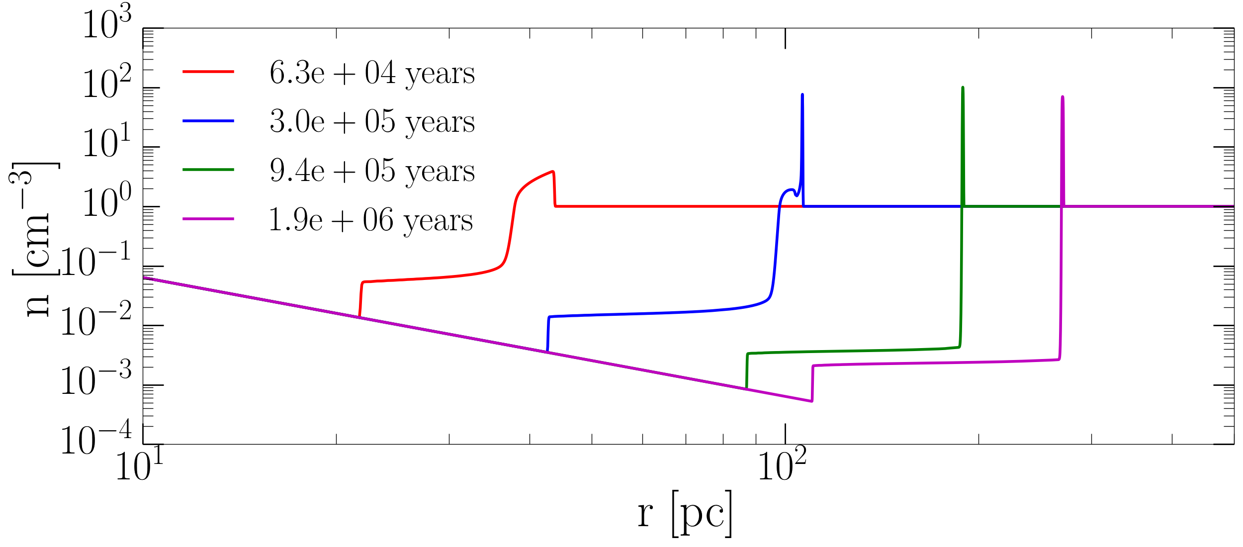
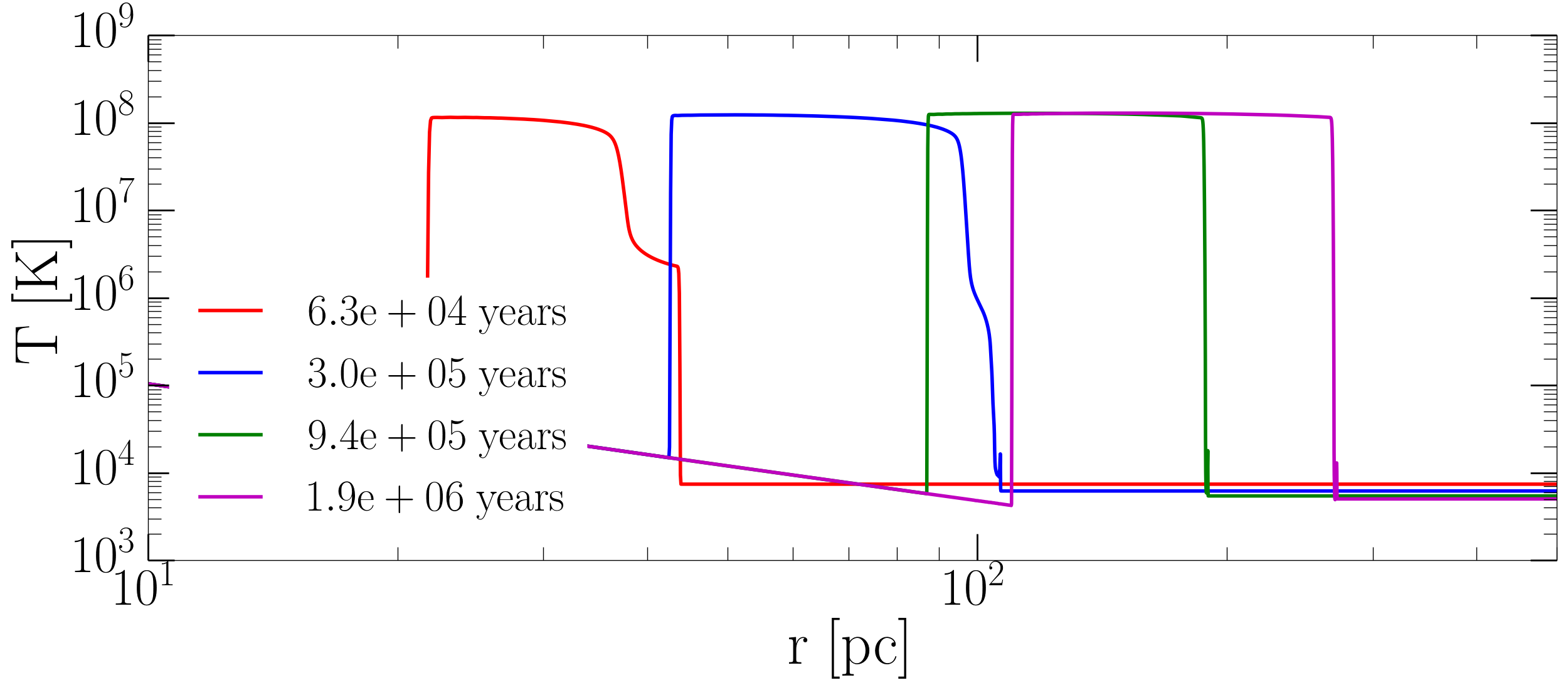
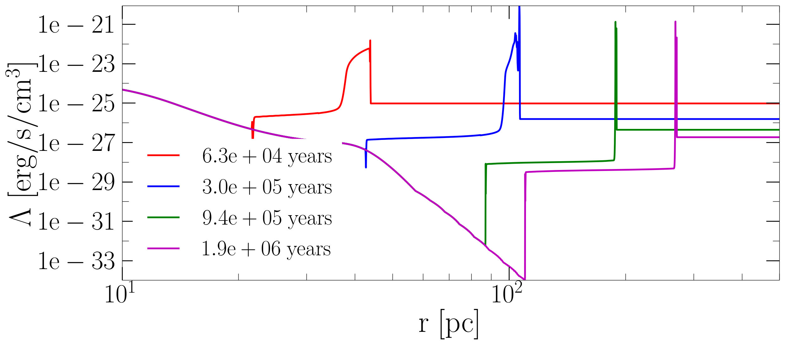
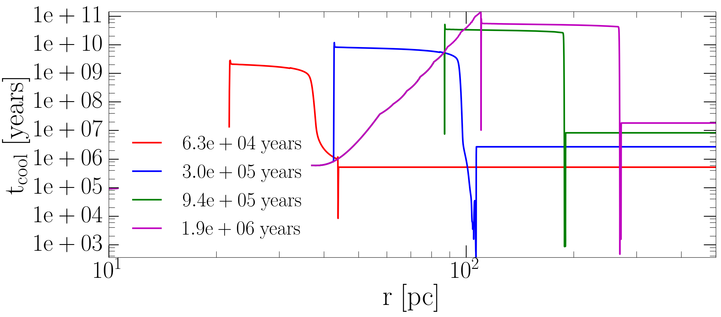
Figure 2: Panels 1-4 respectively show profiles of density, temperature, cooling rate and cooling time scale for the expanding bubble in the fiducial model L40v-2. Four different times are shown. The red line at $t=6.3\times 10^{4}$ years shows an extended layer of shocked ISM, which begins collapsing into a thin shell at $t=3\times 10^{5}$ years (blue line). This marks the transition from the adiabatic to the radiative stage of expansion, where the shocked ISM begins to cool efficiently. The shocked wind remains adiabatic and continues to expand as a thick envelope of tenuous hot gas until late times.

3.1.2 Radiative properties

A bolometric light curve can be calculated directly from KORAL by summing at each instant of time the total cooling over all spherical shells in the ULXB. To calculate light curves in specific frequency bands we need to calculate spectra as a function of time, which we do as follows.

We take the density and temperature profiles directly from the KORAL simulation, and estimate the cooling rate $\Lambda$ for the gas in each cell using Figure 1. For the spectrum emitted from a shell of width $\delta R$ at radius $R$ and temperature $T$, we assume for simplicity that it has the same shape as bremsstrahlung emission and write

$$S_{\rm\nu}={\frac{h\Lambda}{kT}\exp\left({-\frac{h\nu}{kT}}\right)}\times 4\pi R^{2}\delta R.$$ (8)

We note that by normalizing the spectrum with $\Lambda$, the cooling rate obtained by CHIANTI, we include emission via bound-free cooling as well as free-free cooling. Therefore, even though the shape is approximated to a bremsstrahlung spectrum, the overall emission rate is preserved. This is significant because the difference between the cooling rates spans several orders of magnitude for gas at temperatures $\lessapprox 10^{6}$ K, where most of the radiation is emitted as metal lines. By preserving the total emission rate, our bremsstrahlung approximation ought to provide an order-of-magnitude approximation of the integrated luminosities in various bands (X-ray, optical, radio), but it is not suitable for detailed spectral comparisons. In future work we could improve on our spectrum approximation by calculating the line spectrum of the shock-ionized gas in each cell using the APEC code (Smith et al., 2001).

Using our bremsstrahlung approximation, we integrate the spectra over all shells in the shocked ISM and wind, and estimate the total spectrum of the ULX bubble. This direct method of calculating spectra is adequate during the early adiabatic stage of the bubble. Luminosities in individual bands are calculated by integrating the ULXB spectrum over the corresponding frequency ranges.

During the radiative phase, the emission at the front shock is dominated by rapid cooling of the newly swept up and shocked ISM. However, as we discuss in §3.1.3, numerical simulations have trouble resolving the temperature structure of radiative shocks. Typically, when the radiative efficiency of the shocked gas is high, the post-shock gas in the simulation does not achieve the correct temperature but ends up somewhat cooler because of the finite cell size. If we used the simulation data to calculate the spectrum, we would obtain a misleadingly soft spectrum, with its peak at a lower frequency. This is an issue during the radiative phase of the expansion, when the emission is dominated by the front shock. Fortunately, radiative shocks can be treated analytically to compute the correct spectrum (the following discussion follows Draine 2011).

Consider a spherical shock at radius $R$ which moves outward with a radial velocity $v_{\rm sh}$ into a homogeneous ISM with density $\rho_{\rm ISM}$. The rate at which the mass of shocked ISM increases with time is given by

$$\dot{M}_{\rm sh}=4\pi R^{2}v_{\rm sh}\,\rho_{\rm ISM}.$$ (9)

Each parcel of gas is hottest immediately after the shock, where its temperature is given by the adiabatic shock jump conditions. For simplicity, we assume that the external medium is “cold”, which means that the shock velocity is much greater than the sound speed in the medium. This is true for ULX bubbles, since the sound speed in the medium is only about $10~{}{\rm km\,s^{-1}}$, whereas the shock moves at hundreds of $\rm km\,s^{-1}$. Therefore, the immediate post-shock density and pressure are given by,

$$\rho_{2}=\frac{\gamma+1}{\gamma-1}\,\rho_{\rm ISM}=4\rho_{\rm ISM},$$ (10)

$$P_{2}=\frac{2}{\gamma+1}\,\rho_{\rm ISM}v_{\rm sh}^{2}=\frac{3}{4}\,\rho_{\rm ISM}v_{\rm sh}^{2},$$ (11)

where we have set the adiabatic index $\gamma=5/3$. The immediate post-shock temperature is then

$$T_{2}=\frac{\mu m_{\rm p}P_{2}}{k\rho_{2}}=\frac{3}{16}\,\frac{\mu m_{\rm p}}{k}\,v_{\rm sh}^{2},$$ (12)

where $\mu$ is the effective molecular weight of the gas.

Each parcel of gas starts with temperature $\rm T2$ (and density $\rho_{2}$) immediately after it crosses the shock, but it then cools down to a final temperature $\rm T_{3}$ which it reaches far downstream. In our simulations, $T_{3}$ is typically between $4000-8000$ K. The cooling from $T_{2}$ to $T_{3}$ converts thermal energy to radiation, and we can calculate how much radiation is emitted at each temperature.

Immediately post-shock, the downstream gas density is $\rho_{2}=4\rho_{\rm ISM}$ and its velocity is $u_{2}=v_{\rm sh}/4$. However, both $\rho(r)$ and $u(r)$ vary with distance away from the shock because cooling causes the temperature $T(r)$ to vary. Since the mass flux is conserved in the shock frame,

$$\rho(r)u(r)=\rho_{\rm ISM}v_{\rm sh}~{}~{}\to~{}~{}\frac{\rho(r)}{\rho_{\rm ISM}}=\frac{v_{\rm sh}}{u(r)}\equiv x(r),$$ (13)

where $x(r)$ measures the density compression at any given radius r downstream of the shock. (We ignore the spherical geometry in this analysis since the cooling region of the radiative shock is quite thin compared to the local radius.) Momentum flux is also conserved. Ignoring the upstream pressure, this gives

$$\rho(r)u^{2}(r)+P(r)=\rho_{\rm ISM}v_{\rm sh}^{2}~{}~{}\to~{}~{}P(r)=\frac{[x(r)-1]}{x(r)}\,\rho_{\rm ISM}v_{\rm sh}^{2}.$$ (14)

Rewriting in terms of the temperature $T(r)=\mu m_{\rm p}P(r)/kx(r)\rho_{\rm ISM}$, we obtain the following quadratic equation for $x(r)$ as a function of $T(r)$:

$$\frac{kT(r)}{\mu m_{\rm p}}\,x^{2}(r)-v_{\rm sh}^{2}\,x(r)+v_{\rm sh}^{2}=0.$$ (15)

The solution to this equation is

$$x(r)=\frac{\mu m_{\rm p}}{2kT(r)}\left[v_{\rm sh}^{2}+\left(v_{\rm sh}^{4}-4v_{\rm sh}^{2}\frac{kT(r)}{\mu m_{\rm p}}\right)^{1/2}\right],$$ (16)

with

$$\frac{dx}{dT}=\frac{x^{2}(r)}{v_{\rm sh}^{2}-2x(r)kT(r)/\mu m_{\rm p}}.$$ (17)

Consider now the energy equation of the shocked gas and the radiative luminosity. The differential amount of radiation $dE_{\rm rad}$ emitted by unit mass of the gas as its temperature changes from temperature $T$ to $T+dT$ is

$$-dE_{\rm rad}=dQ=du+P(r)d\left[\frac{1}{\rho(r)}\right]=\frac{k}{\mu m_{\rm p}}\left[\frac{3}{2}-\frac{T(r)}{x(r)}\frac{dx}{dT}\right]dT.$$ (18)

Substituting for $x$ and $dx/dT$, and scaling up to the entire volume of the shocked gas, we obtain the total luminosity emitted in a logarithmic temperature interval $\Delta\ln T$,

$$\Delta\dot{U}=4\pi R^{2}v_{\rm sh}\rho_{ISM}\,\frac{kT}{\mu m_{\rm p}}\,\left[\frac{5}{2}+\frac{v_{\rm sh}^{2}-(v_{\rm sh}^{4}-4v_{\rm sh}^{2}kT/\mu m_{\rm p})^{1/2}}{(v_{\rm sh}^{4}-4v_{\rm sh}^{2}kT/\mu m_{\rm p})^{1/2}}\right]\,\Delta\ln{T}.$$ (19)

As before, to calculate the spectrum of this radiation, we assume that the heated gas emits with a spectrum similar to bremsstrahlung radiation. Thus, following equation (8), we write the spectral emission from gas at temperature $T$ as

$$\frac{dL_{\nu}^{ff}}{d\ln T}=\frac{\Delta\dot{U}}{\Delta\ln T}\,\frac{h}{kT}\exp\left(-{\frac{h\nu}{kT}}\right).$$ (20)

Summing up all the spectra over the temperature range from $\rm T_{3}$ to $\rm T_{2}$, we obtain the net spectrum of the forward shock region in the ULXB.

To calculate the spectrum during the radiative phase, we first use directly the density and temperature profiles from the simulation to obtain the spectrum from the shocked wind and the cooled region of the shocked ISM. We then define a cutoff at the temperature minimum of the swept up ISM, and for the region between this cutoff and the location of the forward shock, we follow the analytical approach described above. The gas temperature at the cutoff location is the final temperature $T_{3}$ of the shocked ISM. We calculate the immediate post-shock temperature $T_{2}$ analytically (equation 12) by estimating the shock velocity from KORAL. Then we integrate equation (20) from $T_{2}$ to $T_{3}$ to calculate the analytical spectrum from the radiative forward shock of the bubble.

In Figure 3 we show light curves and spectra corresponding to the fiducial model L40v-2. The initial bolometric and optical luminosities are low. After about $\approx 0.25$ Myrs, the bolometric luminosity begins to increase, reaching $L_{\rm bol}\approx 10^{40}\,{\rm erg\,s^{-1}}$, at 0.5 Myrs. During the adiabatic phase at the start of expansion, the wind luminosity is stored in the shocked wind and ISM. This energy is emitted once the ULXB enters the radiative stage. When the transition to the partially radiative phase is complete (at t $\approx 0.5\,$Myrs) the luminosities in all bands reach a stable value, roughly 50% of the wind mechanical luminosity (comparable to the classical value of 27/77 from bubble theory: Weaver et al. 1977). The radio emission at 5 GHz (black line) stays at $\approx 10^{34}\,{\rm erg\,s^{-1}}$ at early times, and increases by an order of magnitude after 0.3 Myrs.

The bottom panel of Fig. 3 shows computed spectra corresponding to the adiabatic, transition and radiative phases. The adiabatic and transition spectra were obtained purely from the density and temperature profiles from KORAL, whereas the spectrum in the radiative phase is partially from KORAL but using the previously described analytical model for the radiation from the radiative forward shock. The evolution of the spectrum shows that X-ray emission from the ULXB is highest during the initial adiabatic expansion. The bolometric luminosity, on the other hand, is low at early times (as can be seen in the top panel of Figure 3), but the emission peak is shifted towards higher frequencies. By the time the transition to the radiative phase is completed at $\approx 0.5$ Myrs, the X-ray emission has already fallen well below $10^{35}\,{\rm erg\,s^{-1}}$, which is seen also in the spectrum at this time (green lines in the top and bottom panels of Figure 3). At late times the peak of the spectrum has shifted towards the optical/UV regime. The light curves reflect this: While the X-ray luminosity has decreased significantly, the optical emission remains stable at several $10^{39}{\rm\,erg\,s^{-1}}$ throughout the radiative phase.

A pure bremsstrahlung approximation for the shape of the emitted spectrum provides a convenient order-of-magnitude estimate for the shape of the emitted spectrum, especially for the X-ray and radio bands, but it is inadequate to describe the optical spectrum from the shocked ISM layer, for any realistic composition of the ISM. To compare our results with optical observations, we need to insert our model parameters (input mechanical power, $v_{\rm sh}$, ISM density) into a shock-ionization code such as Mappings III (Dopita & Sutherland, 1995, 1996; Allen et al., 2008). Table 2 lists the velocity of the forward shock at characteristic epochs for the various simulated models. As an example, we have used these velocities to calculate and plot (Figure 4) the predicted spectrum of important diagnostic lines, for an input mechanical power of $10^{40}\,{\rm erg\,s^{-1}}$, ISM density of 1$\,\rm{cm^{-3}}$, solar metallicity, and an equipartition magnetic field. For some lines (most notably H$\beta$), the flux is almost independent of shock velocity: such lines are a good proxy for the mechanical power. Instead, other lines (most notably [O I] $\lambda 6300$ and He II $\lambda 4686$) depend strongly on $v_{\rm sh}$. Since our models predict the evolution of $v_{\rm sh}$ as a function of bubble age for a given mechanical power, we can couple our results to a shock-ionization code, and predict the evolution of the optical spectrum and hence the characteristic age of an observed ULXB. This is left to follow-up work.

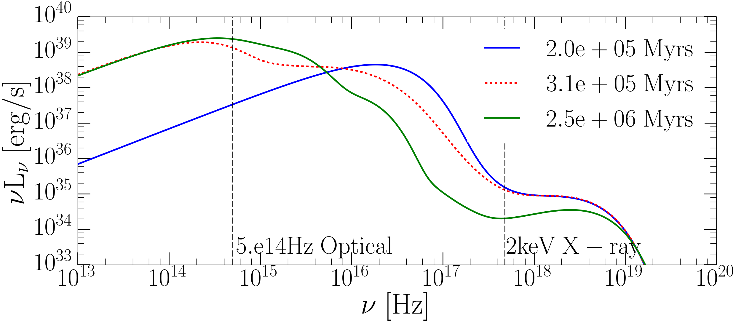
Figure 3: Top: Volume-integrated emission of the ULX bubble in the fiducial run (model L40v-2, $L_{\rm w}=10^{40}\,{\rm erg\,s^{-1}}$, $v_{\rm w}=10^{-2}c$) as a function of time. Red, blue, black and green lines show bolometric, optical ($5\times 10^{14}$ Hz), radio (5 GHz) and X-ray (2 keV) light curves. Bottom: Spectra corresponding to the early adiabatic phase of the forward shock (blue), the transition from adiabatic to radiative (red dashed), and fully radiative (green line).

Table 2: Shock velocities at characteristic epochs

Name	$v_{\rm sh,0.4Myrs}$	$v_{\rm sh,0.5Myrs}$	$v_{\rm sh,1Myrs}$	$v_{\rm sh,2Myrs}$
L40v-1.5	287	191	106	77
L40v-2	287	191	107	78
L40v-2.5	284	191	110	81
L40v-3	152	146	120	89
L39v-2	141	113	69	50
$v_{\rm sh,0.4Myrs}$, $v_{\rm sh,0.5Myrs}$, $v_{\rm sh,1Myrs}$ and $v_{\rm sh,2Myrs}$ are the shock
velocities after 0.4, 0.5, 1 and 2Myrs of bubble expansion,
in $\rm km\,s^{-1}$.

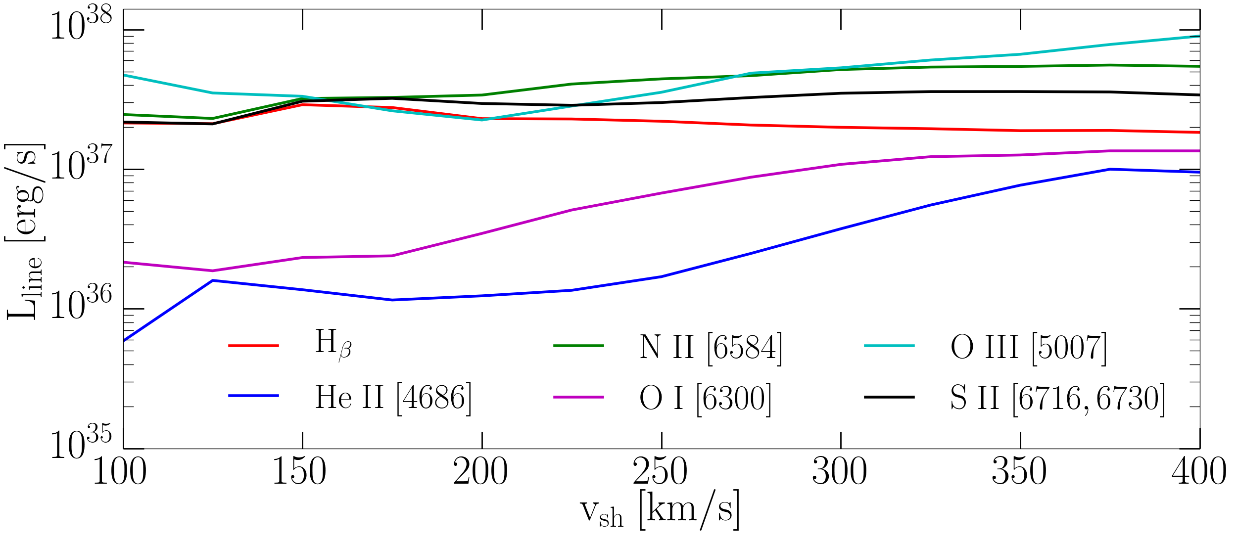
Figure 4: Main diagnostic optical emission line luminosities (He II $\lambda 4686$, H_β, [O III] $\lambda 5007$, [O I] $\lambda 6300$, [N II] $\lambda 6584$ and the doublet [S II] $\lambda 6716,6730$) as a function of shock velocity, predicted for an input mechanical power of $10^{40}{\rm erg\,s^{-1}}$. The luminosities have been calculated with the shock-ionization code Mappings III (Allen et al. 2008), for an ISM density of 1 cm^-3, solar metallicity, and an equipartition magnetic field.

3.1.3 Resolution study

A potential weakness of numerical simulations on fixed grids is that shocks and contact discontinuities (CD) can be under-resolved. We have already discussed the difficulties in simulating radiative shocks. Here we discuss the CD.

Ideally, in the absence of thermal conduction (Weaver et al., 1977), the CD is described by a step function in both density and temperature, with no break in the pressure. However, due to numerical diffusion and finite resolution, simulations are unable to reproduce this sudden break in the density and temperature. The CD is smoothed out over a number of cells containing gas at intermediate temperatures and densities. These intermediate temperatures correspond to the peak of the cooling function (see Figure 1). Since the densities in this region are also fairly high, the simulation would predict a considerable amount of spurious emission from the region surrounding the CD.

Here we compare the profiles and spectra of the forward shock and the CD for the fiducial model L40v-2 during the radiative phase, obtained with low (4608), medium (9216) and high (13824) spatial resolution. In Figure 5 we show the density and temperature profiles (top and middle panels) and the computed spectrum (bottom panel). Although all profiles are calculated at the same time, they are offset spatially. This is due to slightly faster expansion in the higher resolution case during the radiative phase.

Comparison of the density profiles in the top panel of Figure 5 shows a change in CD shape from the lowest resolution (red, 4608) to moderate resolution (blue line, 9216 cells). The moderate and high resolution (blue and green) models are more similar, so we conclude that there is not much to be gained by going above a resolution of $\approx 10000$.

The temperature profile, however, shows that even our highest resolution case does not resolve the radiative forward shock. The temperature of the shocked gas falls well below the analytical post-shock temperature (marked with the horizontal black line). This is a well-known problem (Hutchings & Thomas, 2000; Creasey et al., 2011), and is the reason why we resorted to an analytical method for calculating the spectrum of the shocked ISM.

Comparing the spectra (bottom panel) it is apparent that the lowest resolution case is the brightest in the optical, likely because of poor resolution near the CD. This is not the case in the X-ray band, where the three solutions produce emission at the same level, proving that even the lowest resolution adopted is enough to resolve regions occupied by the hottest gas.

In Figure 5 we show also a model in which we replace the numerical CD with a step function (magenta lines). In this case, the emission in the optical band is lower by a factor of several. However, the X-ray emission is hardly different from the other three spectra, confirming that the X-ray emission is not affected by resolution. The continuum between the optical and X-ray band that is seen in the red, blue and green lines is replaced in the magenta line by a cutoff near $10^{16}$ Hz. Fortunately, this region of the spectrum is not accessible to observations, so the large difference is not a problem. As for the optical emission, the magenta spectrum probably underestimates the true emission because it neglects the effects of heat conduction at the CD (Weaver et al., 1977), so the true answer is probably somewhere between this spectrum and the other three.

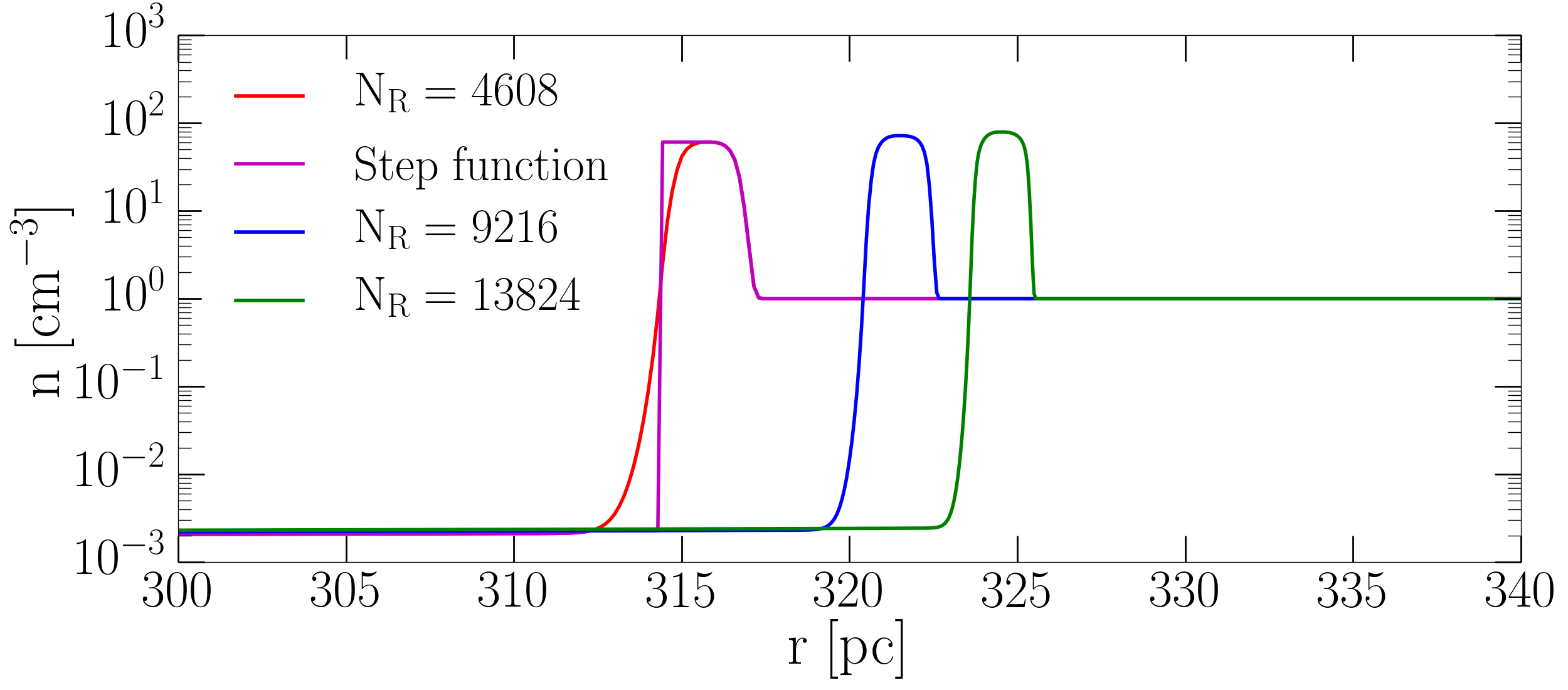
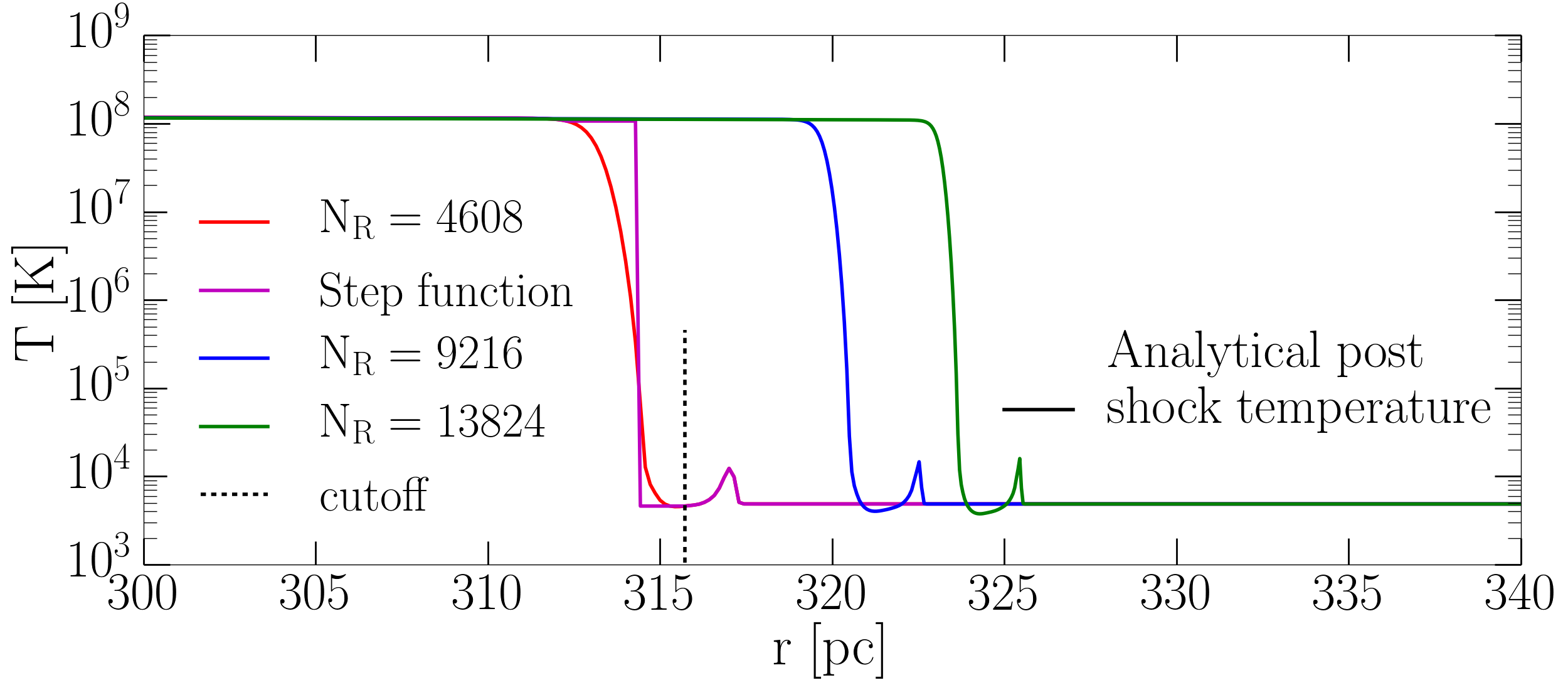
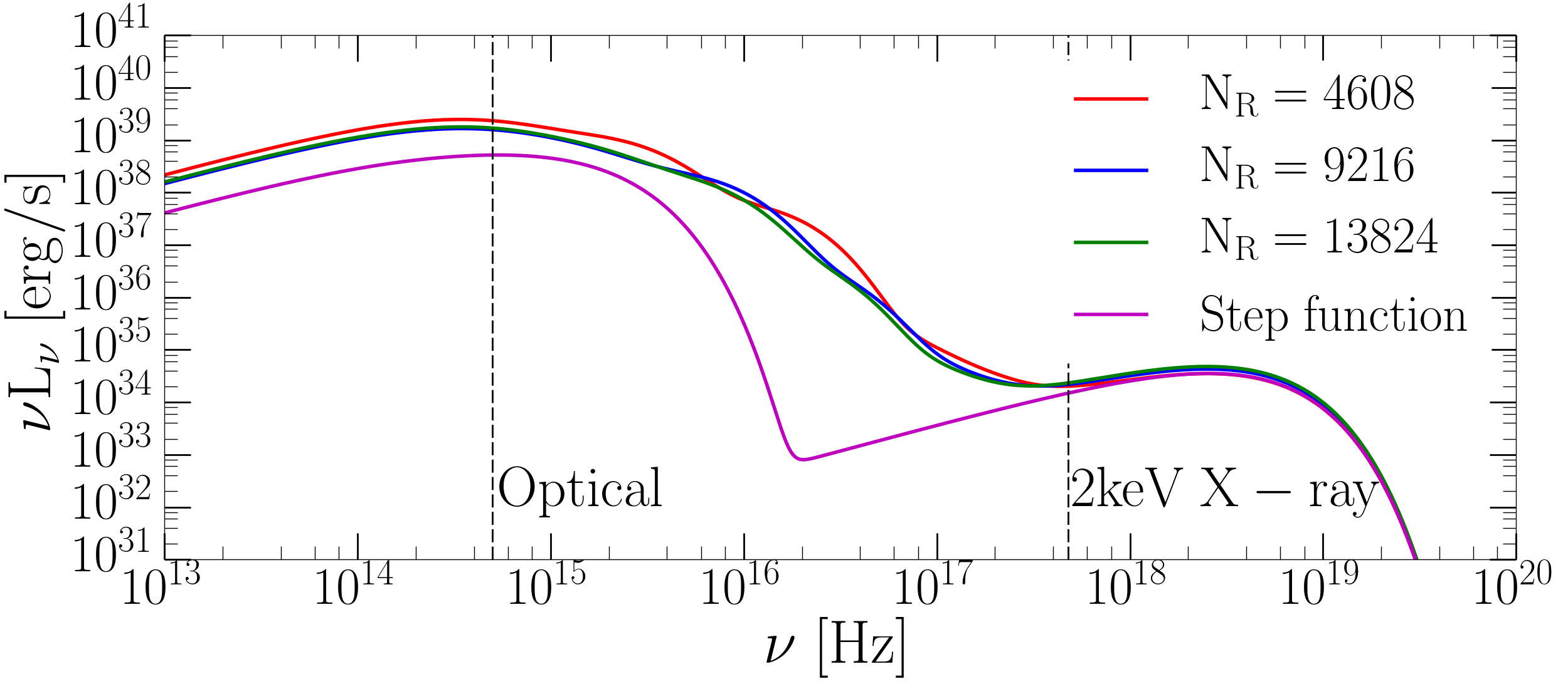
Figure 5: Top and middle panels show the density and temperature through the forward shock and the contact discontinuity in the fiducial model for three different resolutions: $N_{\rm R}=4608$ (red lines), $N_{\rm R}=9216$ (blue lines) and $N_{\rm R}=13824$ (green lines). The magenta line shows an idealized model in which the CD is taken to be a step function. The bottom panel displays corresponding spectra, using the same colors. The step function CD (magenta line) shows considerably less EUV emission.

3.2 Parameter study

3.2.1 Expansion

In Figure 6 we show density and temperature profiles corresponding to the adiabatic, transition and radiative phases for models with $L_{\rm w}=10^{40}\,{\rm erg\,s^{-1}}$ and wind velocities $v_{\rm w}=10^{-1.5}c$, $v_{\rm w}=10^{-2}c$, $v_{\rm w}=10^{-2.5}c$ and $v_{\rm w}=10^{-3}c$ (models L40v-1.5, L40v-2, L40v-2.5, L40v-3).

All four of these ULXB models begin the transition from the adiabatic to the radiative phase at radius $R\approx 100$ pc. There is a clear trend in panels 1-3: As the wind velocity decreases, the density of the shocked wind envelope increases (because the density of the unshocked wind itself increases) while the temperature of the shocked wind decreases (because of the lower wind velocity). The shocked wind temperatures are a few $10^{9}\,$K, $10^{8}\,$K and $10^{7}\,$K for models L40v-1.5, L40v-2, L40v-2.5, respectively. The properties of the shocked ISM are identical in all three cases throughout the ULXB evolution, as are the shock expansion rates.

Panel 4 ($L_{\rm w}=10^{40}$, $v_{\rm w}=10^{-3}c$) shows a qualitative break from the previous pattern. The shocked wind and ISM become radiatively efficient at roughly the same time (again at radius $R\approx 100$  pc), and both zones collapse to a thin, dense shell of cold gas with $\rm T\approx 10^{4}\,K$. This model behaves differently because, given the low wind velocity $v_{\rm w}=0.001c$, the gas crossing the reverse shock heats up to temperatures below $\rm T_{\rm w}\approx 10^{6}\,K$, where the cooling function peaks (Figure 1), causing the shocked wind to collapse through catastrophic cooling. At later stages (purple lines in the bottommost panels of Figure 6) a radiatively inefficient, hot wind layer begins to develop again behind the contact discontinuity. This happens despite the low shocked wind temperature because of decreasing gas density in this regime — the density is no longer large enough to provide efficient cooling.

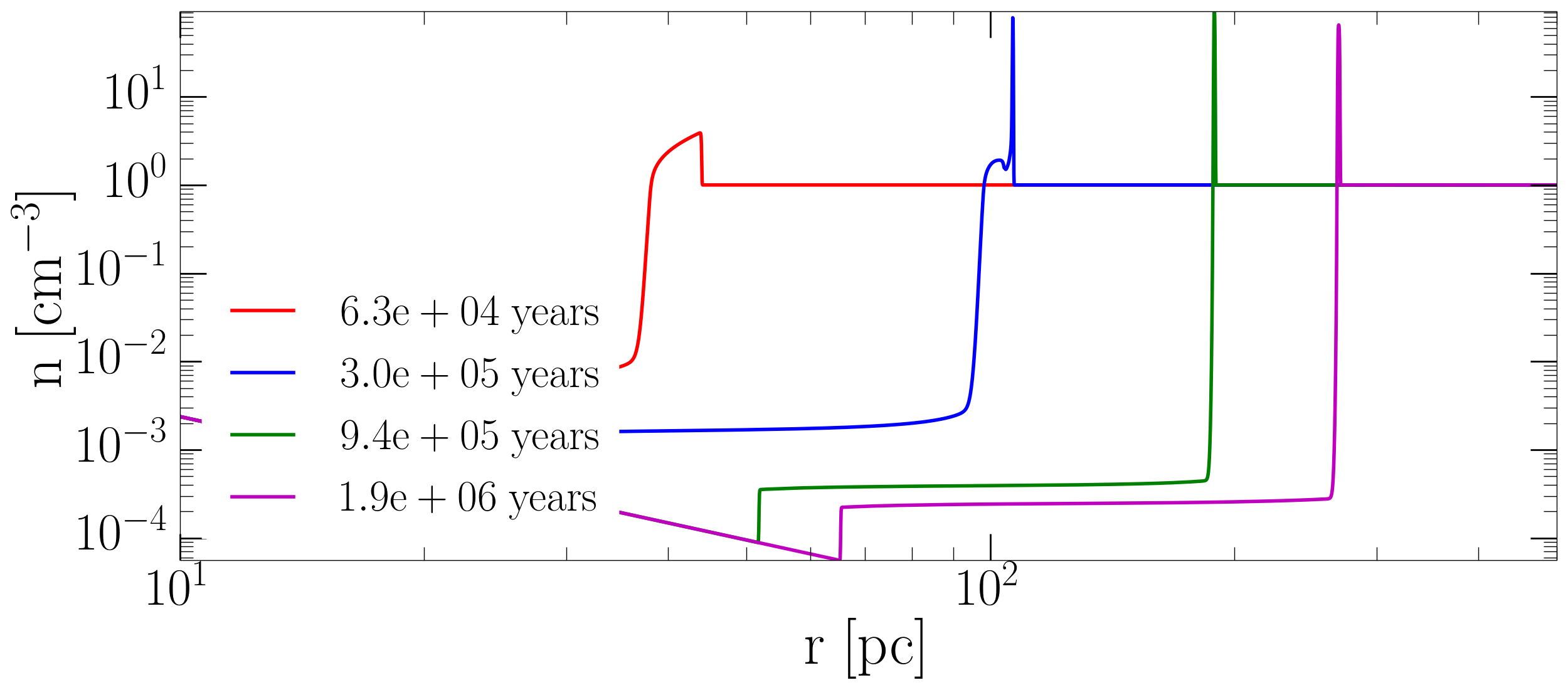
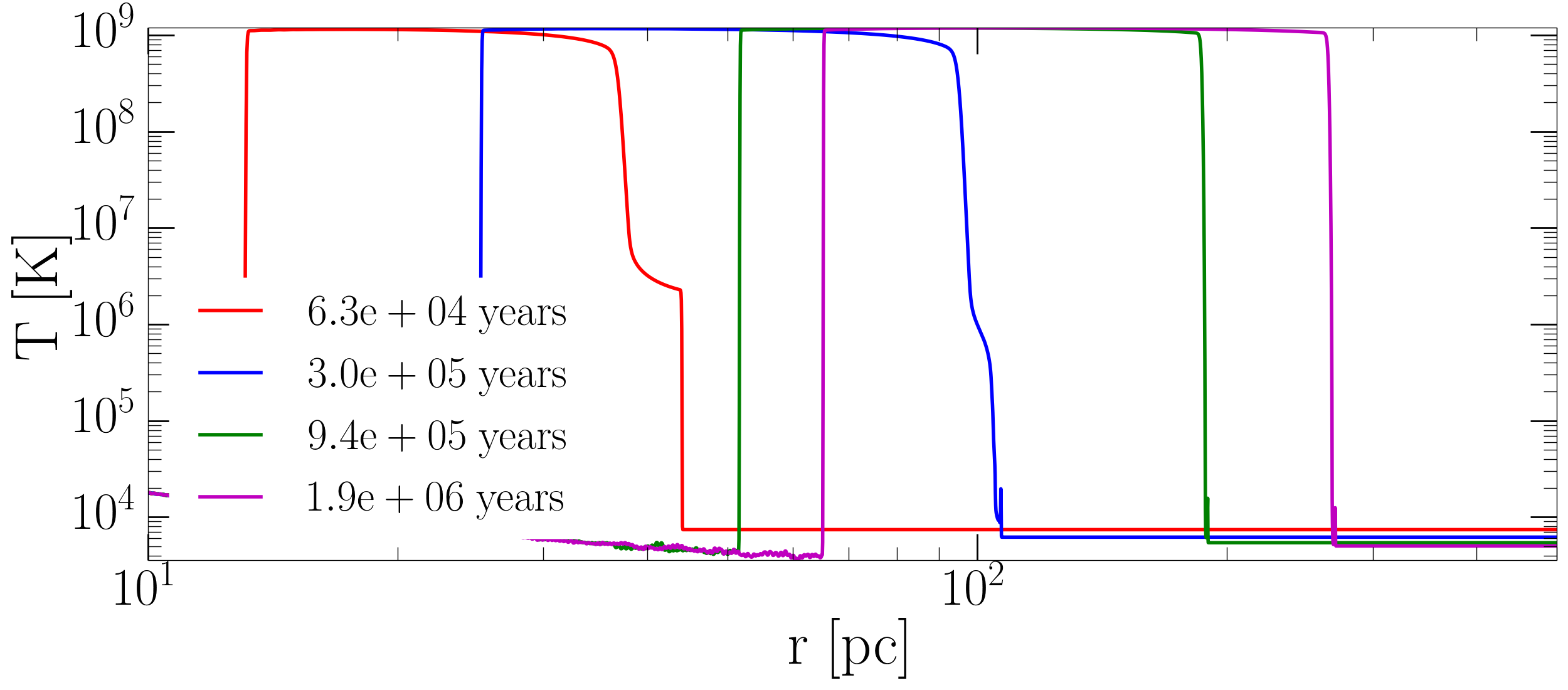
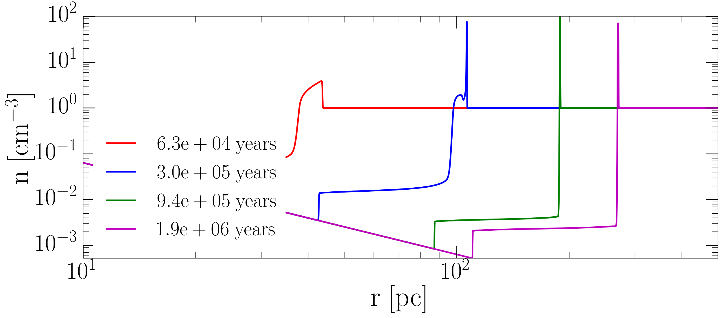
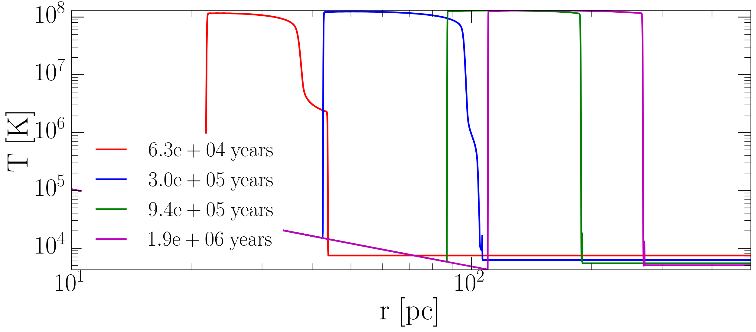
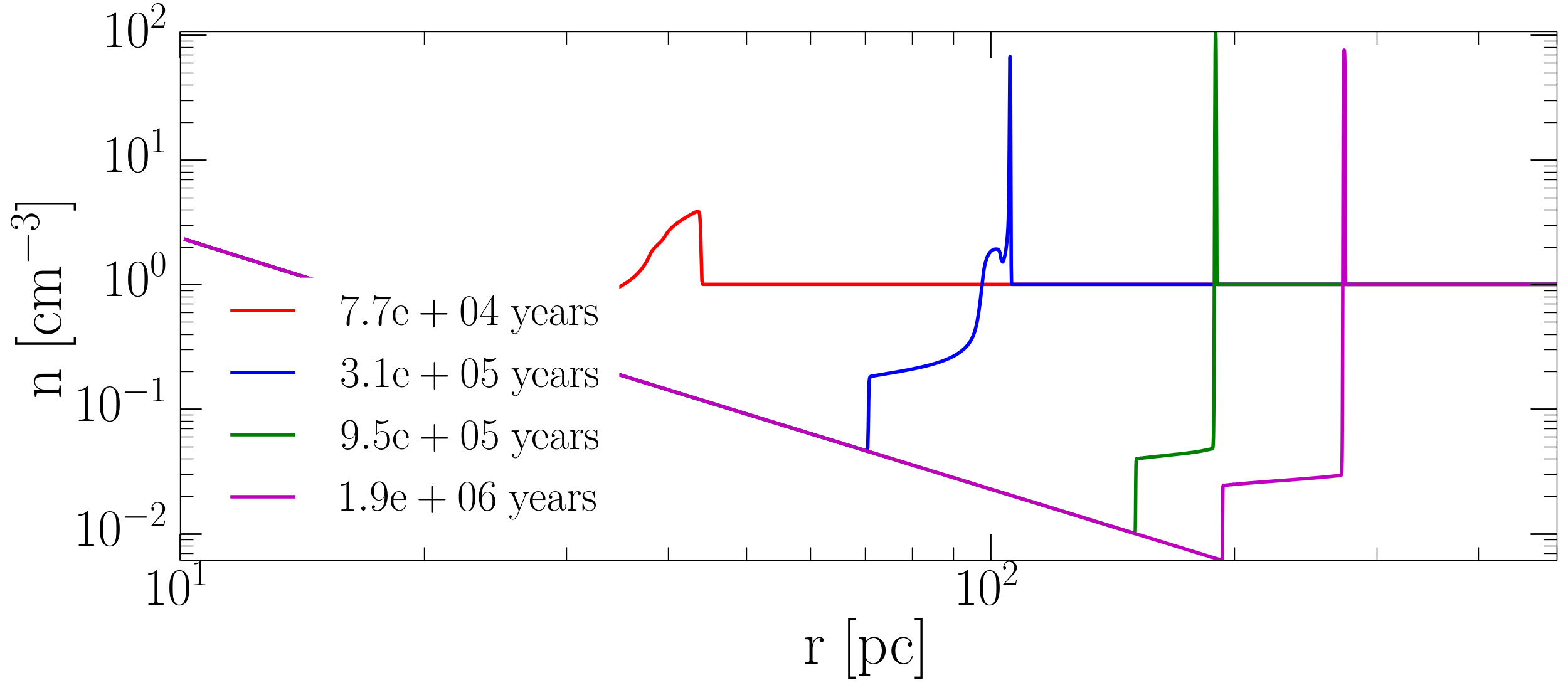
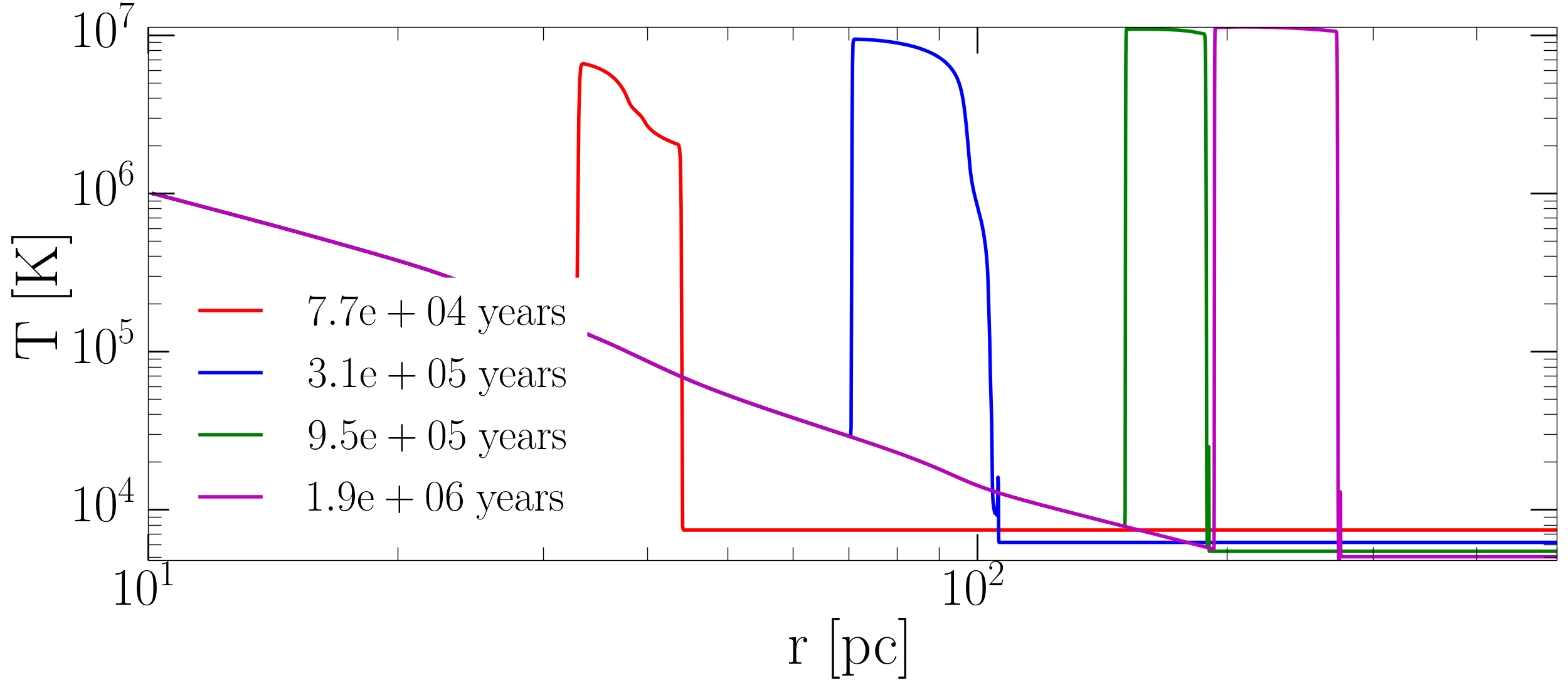
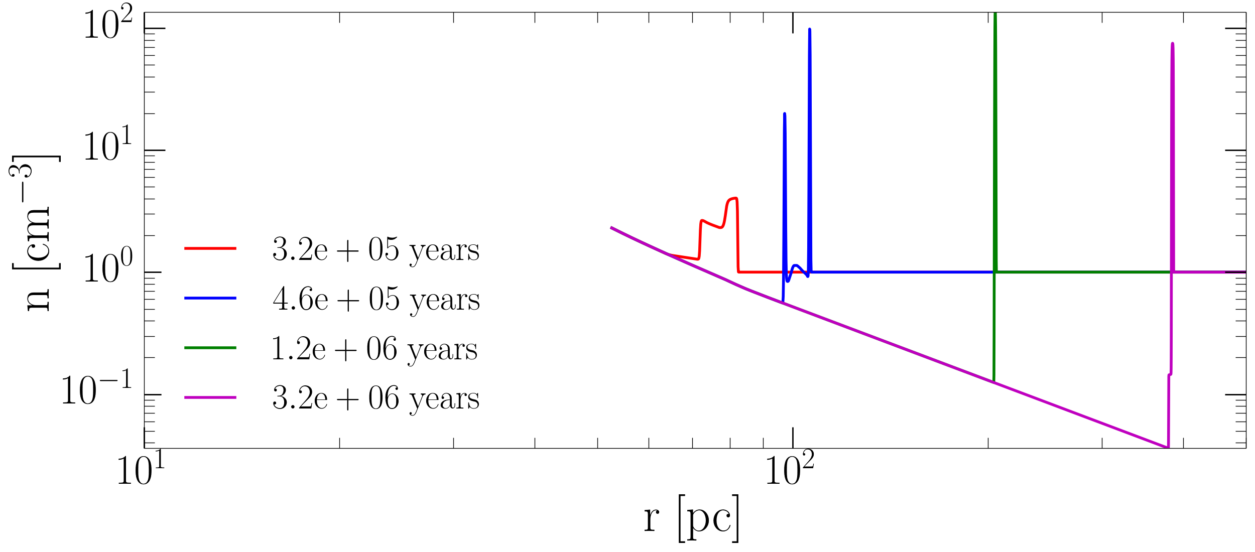
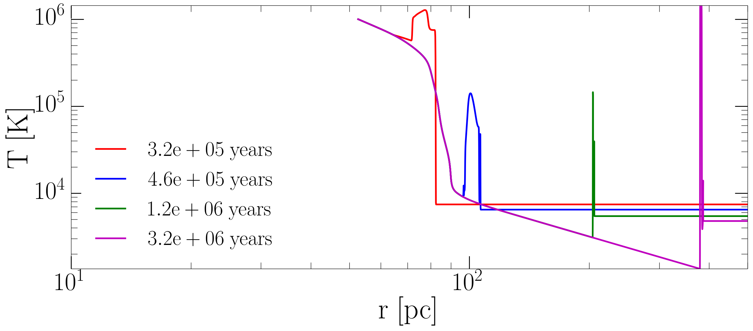
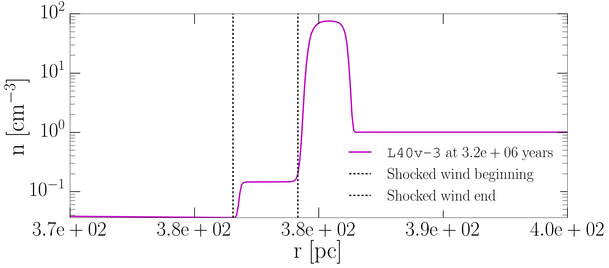
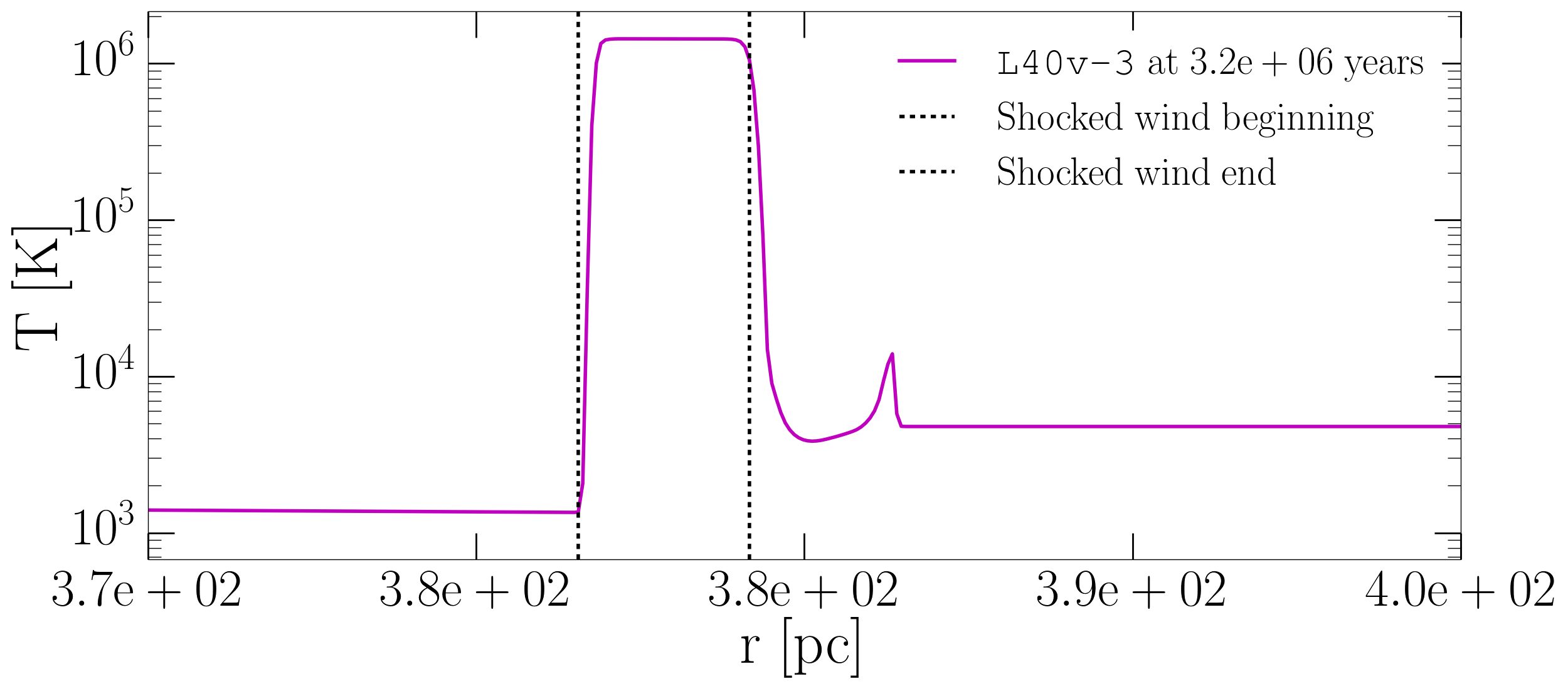
Figure 6: The top four rows show density (left) and temperature (right) profiles through ULXBs with wind luminosity $L_{\rm w}=10^{40}\,{\rm erg\,s^{-1}}$ and wind velocities $v_{\rm w}=10^{-1.5}\,c$, $v_{\rm w}=10^{-2}\,c$, $v_{\rm w}=10^{-2.5}\,c$ and $v_{\rm w}=10^{-3}\,c$, respectively (from top to bottom). Rows 1-3 show the standard three phases: adiabatic expansion (red), transition from adiabatic to radiative expansion (blue), and radiative expansion (green and magenta). All shocks seem to propagate at comparable speeds. However, as the wind velocity decreases, so does the extent of the shocked wind envelope (rows 1-3). In row 4 a small envelope of shocked wind and swept up ISM is visible only at early times (red line). Subsequently, the shocked wind and ISM both simultaneously collapse into thin shells due to efficient cooling (blue line, see discussion in Section 3.2). The snapshots in the fourth row panels are taken at slightly different times compared to the other three models, to better illustrate the characteristic properties of bubble expansion in this regime. In the bottom row, the late stage of the model with $v_{\rm w}=10^{-3}\,c$ is shown, and illustrates the appearance of an adiabatic shocked wind at late times.

3.2.2 Radiative properties

Figure 7 shows the velocity dependence of the total luminosities of the ULXB models during the radiative phase. The bolometric luminosity stays approximately independent of the wind velocity, except for the model with $v_{\rm w}=10^{-3}c$, in which the bolometric luminosity exceeds $10^{40}\,{\rm erg\,s^{-1}}$ slightly (see below). The radiation is emitted predominantly in the UV/optical band, where the luminosity is of order $10^{39}\,{\rm erg\,s^{-1}}$ for all the models, independent of the wind velocity. Similar to the optical, the free-free radio emission does not show significant dependence on wind velocity.

The X-ray emission comes primarily from the shocked wind. It is at most $10^{36}\,{\rm erg\,s^{-1}}$ (in model L40v-2.5), and can be as low as $10^{31}\,{\rm erg\,s^{-1}}$ (in model L40v-3). Although at the highest wind velocities, e.g., $v_{\rm w}=0.03c$ and $v_{\rm w}=0.01c$, the volume of the shocked wind is largest and the temperature is highest (see Figure 6), the X-ray luminosities of these models are low. The reason is that the amount of X-ray emission is a trade off between shocked wind volume, temperature and density.

The emissivity at X-ray temperatures scales as $\epsilon\sim n^{2}T^{1/2}$, hence the X-ray luminosity $L_{X}$ of the bubble scales as

$$L_{X}=\epsilon V\sim n^{2}T^{1/2}V,$$ (21)

where $V$ is the volume of the shock-heated gas. Going from model L40v-1.5 ($v_{\rm w}=0.03c$) to model L40v-2.5 ($v_{\rm w}=0.003c$), the temperature decreases by two order of magnitude, but the density increases by two orders of magnitude. Since density has a much stronger effect on the emissivity, the result is that the model with the slower wind has a substantially larger $L_{X}$. This trend continues until the wind velocity is so low that the gas temperature falls below the X-ray band. This is the case with model L40v-3, which has almost no X-ray emission. The net result is that $L_{X}$ is largest for $v_{\rm w}=0.003c$, which is still hot enough for X-ray emission ($>10^{6}\,$K), and has the largest density among the models that satisfy this requirement.

In model L40v-3, the shocked wind is radiatively efficient and the gas cools considerably. Therefore, the model radiates predominantly in the UV and optical. This emission is responsible for the much higher bolometric luminosity of this model. In fact, the radiative luminosity is slightly above $10^{40}\,{\rm erg\,s^{-1}}$ (the injected wind kinetic luminosity) during the radiative phase (Figure 7). The extra luminosity results from the emission of thermal energy accumulated during the adiabatic phase.

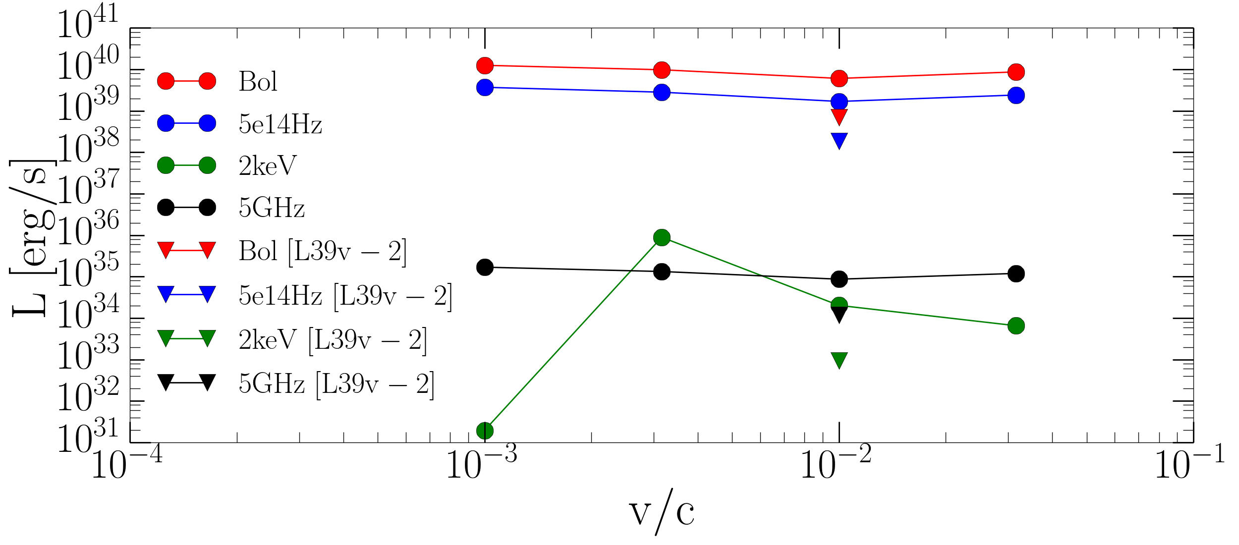
Figure 7: Bolometric, optical ($5\times 10^{14}$ Hz), radio (5GHz) and X-ray (2 keV) emission of the ULXB as a function of wind velocity. All luminosities are taken from the radiative phases of the ULX bubble at $\approx 2\,$Myrs. For $v_{\rm w}=10^{-3}c$ the shocked wind cools efficiently and no significant X-ray emission is observed.

4 Discussion

4.1 Range of validity of the simulations

As we mentioned in Section 1, ULXs affect the surrounding ISM both via X-ray photoionization and via shock-ionization. In this work, we modelled the case of shock-ionized nebulae formed by continuous outflow. Our simulations are based on a number of simplifying assumptions. To start with, we simulated the expanding nebulae assuming perfect isotropy. This is never satisfied in reality. Although the outflow from the accreting system will carry an imprint of the accretion flow geometry, the ISM is never a uniform medium, and fluctuations in its density will affect the expansion of the nebula, making it highly non-isotropic.

Radiative shocks are known to be subject to thermal and thin-shell instabilities (Vishniac, 1983; Chevalier & Imamura, 1982), and we therefore tested our model for Rayleigh-Taylor (R-T) instabilities by running 2-D simulations. We did not detect any instabilities, though this may be due to the low spatial resolution we employed. Previous studies such as Porth et al. (2014) did observe the development of R-T filaments in adaptive mesh refinement MHD simulations of pulsar wind nebulae, but those simulations used much higher (> 1 order of magnitude) resolution compared to ours. If R-T instabilities occur, we might expect the cold ISM to mix with the hot shocked wind in the ULXB. The mixing could cool the shocked wind enough to put it in the temperature regime of effective cooling ($\lessapprox 10^{6}$ K), thus shortening the adiabatic expansion phase of the ULXB. In future work high resolution 2-D simulations should be considered to test the effects of instabilities on emission spectra and luminosities of ULXBs in the radiative phase.

In the present work we also neglected the presence of a relativistic, magnetized and collimated BH jet, predicted by MHD simulations as one of the hallmarks of the super-Eddington accretion regime (Sądowski et al., 2014; McKinney et al., 2014; Sądowski & Narayan, 2015; Kawashima et al., 2012; Narayan et al., 2017). Relativistic jets have been detected or inferred so far for a small number of (candidate) super-Eddington stellar-mass BHs: most notably SS 433 (Zealey et al., 1980; Fabrika, 2006), Holmberg II X-1 (Cseh et al., 2013), and the ultraluminous supersoft source in M 81 (Liu et al., 2015). It is still unknown whether all super-critical BHs have jets, and whether the jet power depends on BH spin and on the magnetic configuration near the BH horizon. A jet carries most of its energy in a small opening angle, leading to the formation of an elongated nebula with lobes and hot spots (as observed in the ULX bubble NGC 7793 S26, Pakull et al. (2010) and Soria et al. (2010)). Even when jets are present, MHD simulations of BH accretion predict that a comparable amount of power is carried by wide-angle, slower outflows (Sadowski et al., 2013): in that case, the likely effect on the ISM is a more spherical bubble inflated primarily by the slower wind, with jet-inflated lobes sticking out of the bubble (similar to the morphology of the SS 433/W50 nebula). Our spherically-symmetric model would then more properly apply only to the spherical component of the bubble.

Since we are primarily concerned with wide-angle, massive, slower outflows, we limited our simulations to wind velocities between $0.001c$ and $0.03c$; the narrow jet component is the only part of the outflow that can reach speeds $\gtrsim 0.1c$. Physically, the lower limit of our wind velocity interval corresponds to a threshold where the shocked wind region becomes radiatively efficient and collapses to a thin, dense shell with $T\sim 10^{4}$ K. The upper limit of our velocity interval does not correspond to any physical thresholds; it is the escape velocity of outflows launched from a disk radius $\approx 2000R_{\rm g}$.

Another consequence of our focus on wind-inflated rather than jet-inflated bubbles is that the radio luminosity calculated in Section 3.1.2 includes only the contribution from thermal free-free emission. If a jet is present, we expect also synchrotron emission from relativistic electrons in the lobes and hot spots. For powerful jets, such a component may dominate over the free-free component (as is the case for example in NGC 7793-S26: Soria et al. (2010)). Since we ignore synchrotron radiation, our radio luminosity estimates should be viewed as lower limits to the observable radio emission. If the radio comes primarily from a jet ($v\geq 0.1\,c$) then, extrapolating Cavagnolo et al. (2010) to the typical jet power in ULXs, we estimate that

$$L_{\rm radio}\sim 10^{-5}\times P_{\rm jet}.$$ (22)

We therefore expect synchrotron radio luminosities of order $\sim 10^{35}\rm\,erg\,s^{-1}$ in jet-dominated ULXBs. This is supported by radio observations of the ULX bubbles S26 in NGC7793 (Soria et al., 2010) and MQ1 in M83 (Soria et al., 2014). On the other hand, ULXBs such as Ho IX X-1 and NGC1313 X-2 are just as large and optically luminous, but have low radio luminosities, consistent with just thermal bremsstrahlung emission. It is likely that radio-loud ULXBs are inflated by jets, and radio-quiet ULXBs by winds: for the same amount of kinetic power, jet shocks may be more efficient than winds in accelerating non-thermal electrons. If so, then our calculations give a baseline radio luminosity in the absence of jets, and any synchrotron jet component would be on top of that.

We did not include conduction in our simulations. Weaver et al. (1977) calculated the evaporation of shocked ISM into the shocked wind layer due to conduction, and concluded that 60% of the mass in the shocked wind comes from evaporation across the CD. Conduction can therefore alter the shape of the CD, and the observed spectral properties. The expansion speed of the shock would also be affected. We implicitly assumed that conduction is negligible.

We also do not consider possible non-thermal support by cosmic rays accelerated at the shock or by magnetic fields. Castro et al. (2011) compare the evolution of supernova remnants with and without efficient cosmic ray production and show that cosmic ray production results in higher compression ratios and lower post-shock temperatures, and shocks with smaller radius and speed, as well as lower intensity X-ray thermal emission. These observational properties can be fit to a model with a different set of parameters, in particular a much lower explosion energy, compared to models that include cosmic ray production. In future work we could account for the effects of cosmic ray production on the emitted X-ray spectrum in ULXBs by using a non-equilibrium ionization collisional plasma model, contained in XSPEC (Arnaud, 1996).

We further treated the gas behind the front shock as a single temperature plasma, rather than tracking proton and electron temperatures separately. Recent work on AGN outflows (Faucher-Giguère & Quataert, 2012) has shown that proton cooling timescales can exceed electron cooling timescales significantly, and thus increase the parameter range over which such outflows are adiabatic. It would be interesting to rerun the simulations reported here using separate cooling functions for electrons and protons.

4.2 Diagnostics of wind speed

The standard model of the expansion of a wind-inflated nebula predicts that the properties of the shocked ISM depend only on the mechanical luminosity of the outflow. In particular, shell temperature and luminosity do not depend on the density or velocity of the outflow. The evolution of the swept-up ISM shell in our simulations is consistent with this picture.

The properties of the gas that crosses the reverse shock and forms the hot and tenuous expanding envelope behind the CD are, on the other hand, sensitive to the BH wind properties. For higher wind speeds (and therefore, at a fixed mechanical luminosity, for lower wind densities), post-shock temperatures are larger. The slowest wind speed in our simulations corresponds to the lowest temperature, but also to the highest integrated emission (Fig. 7) because of the shape of the cooling function between $T\sim 10^{5}$–$10^{8}$ K.

By simulating the bubble expansion numerically using a realistic cooling function we were able to extend this classical picture to the regime where the post-shock wind temperature becomes low, bound-free emission becomes effective and the envelope of the shocked wind cools efficiently and collapses to a thin layer, just behind the swept-up ISM shell. In this case the radiative properties of the shocked wind change dramatically, leading to efficient emission in optical wavelengths rather than in X-rays.

This peculiar dependence of the X-ray emission and of the X-ray/radio luminosity ratio on the outflow properties (Fig. 7) could enable us, in principle, to disentangle outflow rate and velocity. For a given nebula it is relatively straightforward to estimate the mechanical power required to inflate the observed cavity. If, in addition, limits can be placed on the X-ray emission from within the bubble, then the unshocked wind velocity may be recovered. This would in turn constrain the outflow densities. Both parameters provide key constraints to MHD simulations of the accretion flow in the innermost region around the BH. The dependence of the X-ray spectrum on wind speed is even stronger if we use more realistic thermal-plasma emission models (e.g., the APEC model: Smith et al. (2001)), including metal lines in addition to free-free emission. In practice, diffuse X-ray luminosity at the level of $L_{\rm X}\lesssim 10^{36}\,{\rm erg\,s^{-1}}$ from ULXBs located at least several Mpc away would require exposure times above 2 Ms to be detected.

5 Summary

We performed one-dimensional simulations of expanding shock-ionized bubbles powered by ULX outflows. We accounted for realistic radiative losses by implementing a cooling function that includes both free-free and bound-free opacities. We studied the properties of the nebular expansion as a function of the mechanical luminosity and velocity of the ULX outflow. We found that:

(i) Consistent with standard analytical models of expanding, wind-driven bubbles, the swept-up, shocked ISM quickly enters the radiative phase and collapses into a thin shell, with peak radiative emission in the optical band and integrated luminosity comparable to the mechanical output of the ULX. The properties of the shocked ISM depend only on the input power (via the shock velocity $v_{\rm sh}$), and not on the velocity or density of the wind.

(ii) For models L40v-1.5, L40v-2 and L40v-2.5, the shock velocity decreases with time, from characteristic values $v_{\rm sh}\approx 300\,$km s^-1 at an age $\approx 10^{5}\,$yr to $v_{\rm sh}\approx 100\,$km s^-1 at an age $\approx 10^{6}\,$yr (Table 2). The value of $v_{\rm sh}$ is the main parameter required to predict realistic optical/UV line emission spectra of the bubble as a function of time. The range of $v_{\rm sh}$ found in our models is consistent with those inferred from the line spectra observed in large ULXBs (Pakull & Mirioni, 2002; Pakull et al., 2005a; Moon et al., 2011). By modelling the evolution of $v_{\rm sh}$ in time, we provide an independent method to determine the age of a ULXB, via its optical line ratios.

(iii) An envelope of shocked wind develops behind the contact discontinuity, again in agreement with the standard models. Contrary to the shocked ISM, the properties of the shocked wind do depend on the input parameters (wind speed and density); higher wind velocities correspond to lower densities and higher temperatures. The shocked wind does not cool efficiently if the wind velocity $v_{\rm w}\gtrsim 0.003c$, leading to temperatures $\sim 10^{7}$–$10^{8}\,$K and X-ray emission. For an input mechanical power $L_{\rm w}=10^{40}\,{\rm erg\,s^{-1}}$, the characteristic bremsstrahlung luminosity at 2 keV is negligible for wind speeds $v_{\rm w}\approx 0.001c$, peaks at $L_{\rm X}\approx 10^{36}\,{\rm erg\,s^{-1}}$ for $v_{\rm w}\approx 0.003c$ ($T\approx 10^{7}$ K), and decreases to $L_{\rm X}\approx 10^{34}\,{\rm erg\,s^{-1}}$ for $v_{\rm w}\approx 0.03c$ ($T\approx 10^{9}\,$K).

(iv) For a given input mechanical power, the free-free radio luminosity (integrated over the whole volume of the bubble) is almost independent of wind velocity; instead, it is a function of bubble age. For a mechanical power of $10^{40}\,{\rm erg\,s^{-1}}$, the 5-GHz luminosity is $\lesssim 10^{34}\,{\rm erg\,s^{-1}}$ in bubbles younger than $\approx 3\times 10^{5}$ yr, and jumps to $\approx 10^{35}\,{\rm erg\,s^{-1}}$ after that. At a characteristic distance of 5 Mpc, this corresponds to a 5-GHz flux density $\lesssim$70 $\mu$Jy for a younger bubble, and $\approx$700 $\mu$Jy for an older bubble. What we calculated here are the minimum levels of radio luminosity expected for a ULXB: they include only free-free emission, not the optically-thin synchrotron emission from the possible jet lobes and hot spots. A small sample of observed ULX jets with powers $\approx 10^{40}\,{\rm erg\,s^{-1}}$ suggests that the jet-powered synchrotron emission at 5 GHz is also $\sim 10^{35}\,{\rm erg\,s^{-1}}$ (Soria et al., 2010, 2014; Cseh et al., 2012).

(v) If the disk outflow velocity $v_{\rm w}\lesssim 0.001c$, the wind that crosses the reverse shock heats up only to moderate temperatures, low enough to allow for efficient bound-free cooling. As a result, the shocked wind cools down and collapses, similarly to the behaviour of the shocked ISM. Instead of having a thin shell of ISM surrounding an extended envelope of hot shocked wind, now there are two thin and cool shells, both emitting efficiently in the optical band. During this phase, the total luminosity is approximately equal to the mechanical energy injection rate; there is no X-ray emission owing to the efficient cooling and low temperatures of both the shocked ISM and shocked wind layers.

6 Acknowledgements

MS and RN were supported in part by NSF grant AST1312651. RN was also funded by the Black Hole Initiative at Harvard University, which is supported by a grant from the John Templeton Foundation. AS acknowledges support from NASA through Einstein Postdoctoral Fellowship number PF4-150126 awarded by the Chandra X-ray Center, which is operated by the Smithsonian Astrophysical Observatory for NASA under contract NAS8-03060. TPR acknowledges support from STFC as part of the consolidated grant ST/L00075X/1. The authors acknowledge computational support from NSF via XSEDE resources (grant TG-AST080026N).

References

- Abolmasov et al. (2007) Abolmasov, P., Fabrika, S., Sholukhova, O., & Afanasiev, V. 2007, Astrophysical Bulletin, 62, 36
- Allen et al. (2008) Allen, M. G., Groves, B. A., Dopita, M. A., Sutherland, R. S., & Kewley, L. J. 2008, The Astrophysical Journal Supplement Series, 178, 20
- Arnaud (1996) Arnaud, K. A. 1996, XSPEC : THE FIRST TEN YEARS, Vol. 101 (Astronomical Society of the Pacific), 17
- Bachetti et al. (2014) Bachetti, M., Harrison, F. A., Walton, D. J., et al. 2014, Nature, 514, 202
- Castor et al. (1975) Castor, J., Weaver, R., & McCray, R. 1975, The Astrophysical Journal, 200, L107
- Castro et al. (2011) Castro, D., Slane, P., Patnaude, D. J., & Ellison, D. C. 2011, The Astrophysical Journal, 734, 85
- Cavagnolo et al. (2010) Cavagnolo, K. W., McNamara, B. R., Nulsen, P. E. J., et al. 2010, The Astrophysical Journal, 720, 1066
- Chevalier & Imamura (1982) Chevalier, R. A., & Imamura, J. N. 1982, The Astrophysical Journal, 261, 543
- Creasey et al. (2011) Creasey, P., Theuns, T., Bower, R. G., & Lacey, C. G. 2011, MNRAS, 415, 3706
- Cseh et al. (2012) Cseh, D., Corbel, S., Kaaret, P., et al. 2012, ApJ, 749, 17
- Cseh et al. (2013) Cseh, D., Kaaret, P., Corbel, S., et al. 2013, MNRAS, arXiv:1311.4867
- Davis et al. (2011) Davis, S. W., Narayan, R., Zhu, Y., et al. 2011, ApJ, 734, 111
- Dere et al. (1997) Dere, K. P., Landi, E., Mason, H. E., Fossi, B. C. M., & Young, P. R. 1997, Astronomy and Astrophysics Supplement Series, 125, 149
- Dopita & Sutherland (1995) Dopita, M. A., & Sutherland, R. S. 1995, The Astrophysical Journal, 455, 468
- Dopita & Sutherland (1996) —. 1996, The Astrophysical Journal Supplement Series, 102, 161
- Draine (2011) Draine, B. T. 2011, Physics of the Interstellar and Intergalactic Medium (Princeton Series in Astrophysics) (Princeton University Press)
- Fabrika (2006) Fabrika, S. 2006, Astrophys. Space Phys. Reviews, 12
- Farrell et al. (2009) Farrell, S. A., Webb, N. A., Barret, D., Godet, O., & Rodrigues, J. M. 2009, Nature, 460, 73
- Faucher-Giguère & Quataert (2012) Faucher-Giguère, C.-A., & Quataert, E. 2012, Monthly Notices of the Royal Astronomical Society, 425, 605
- Feng & Soria (2011) Feng, H., & Soria, R. 2011, New Astron. Rev., 55, 166
- Fürst et al. (2016) Fürst, F., Walton, D. J., Harrison, F. A., et al. 2016, ApJ, 831, L14
- Gladstone et al. (2009) Gladstone, J. C., Roberts, T. P., & Done, C. 2009, MNRAS, 397, 1836
- Hutchings & Thomas (2000) Hutchings, R. M., & Thomas, P. A. 2000, MNRAS, 319, 721
- Israel et al. (2016) Israel, G. L., Belfiore, A., Stella, L., et al. 2016, ArXiv e-prints, arXiv:1609.07375 [astro-ph.HE]
- Kaaret & Corbel (2009) Kaaret, P., & Corbel, S. 2009, ApJ, 697, 950
- Kaaret et al. (2004) Kaaret, P., Ward, M. J., & Zezas, A. 2004, MNRAS, 351, L83
- Kawashima et al. (2012) Kawashima, T., Ohsuga, K., Mineshige, S., et al. 2012, The Astrophysical Journal, 752, 18
- Liu et al. (2013) Liu, J.-F., Bregman, J. N., Bai, Y., Justham, S., & Crowther, P. 2013, Nature, 503, 500
- Liu et al. (2015) Liu, J.-F., Bai, Y., Wang, S., et al. 2015, Nature
- McKinney et al. (2014) McKinney, J. C., Tchekhovskoy, A., Sadowski, A., & Narayan, R. 2014, Monthly Notices of the Royal Astronomical Society, 441, 3177
- Mezcua et al. (2015) Mezcua, M., Roberts, T. P., Lobanov, A. P., & Sutton, A. D. 2015, MNRAS, 448, 1893
- Middleton et al. (2015) Middleton, M. J., Heil, L., Pintore, F., Walton, D. J., & Roberts, T. P. 2015, MNRAS, 447, 3243
- Moon et al. (2011) Moon, D.-S., Harrison, F. A., Cenko, S. B., & Shariff, J. A. 2011, ApJ, 731, L32
- Motch et al. (2014) Motch, C., Pakull, M. W., Soria, R., Grisé, F., & Pietrzyński, G. 2014, Nature, 514, 198
- Narayan et al. (2017) Narayan, R., Sadowski, A., & Soria, R. 2017, ArXiv e-prints, arXiv:1702.01158 [astro-ph.HE]
- Pakull et al. (2005a) Pakull, M. W., Grisé, F., & Motch, C. 2005a, Proceedings of the International Astronomical Union, 1, 293
- Pakull et al. (2005b) —. 2005b, Proceedings of the International Astronomical Union, 1, 293
- Pakull & Mirioni (2002) Pakull, M. W., & Mirioni, L. 2002, ArXiv Astrophysics e-prints, astro-ph/0202488
- Pakull et al. (2010) Pakull, M. W., Soria, R., & Motch, C. 2010, Nature, 466, 209
- Pinto et al. (2016) Pinto, C., Middleton, M. J., & Fabian, A. C. 2016, Nature, 533, 64
- Porth et al. (2014) Porth, O., Komissarov, S. S., & Keppens, R. 2014, Monthly Notices of the Royal Astronomical Society, 443, 547
- Poutanen et al. (2007) Poutanen, J., Lipunova, G., Fabrika, S., Butkevich, A. G., & Abolmasov, P. 2007, MNRAS, 377, 1187
- Ramsey et al. (2006) Ramsey, C. J., Williams, R. M., Gruendl, R. A., et al. 2006, ApJ, 641, 241
- Roberts et al. (2003) Roberts, T. P., Goad, M. R., Ward, M. J., & Warwick, R. S. 2003, MNRAS, 342, 709
- Sądowski & Narayan (2015) Sądowski, A., & Narayan, R. 2015, Monthly Notices of the Royal Astronomical Society, 453, 3214
- Sądowski et al. (2014) Sądowski, A., Narayan, R., McKinney, J. C., & Tchekhovskoy, A. 2014, Monthly Notices of the Royal Astronomical Society, 439, 503
- Sadowski et al. (2013) Sadowski, A., Narayan, R., Penna, R., & Zhu, Y. 2013, Monthly Notices of the Royal Astronomical Society, 436, 3856
- Sądowski et al. (2013) Sądowski, A., Narayan, R., Tchekhovskoy, A., & Zhu, Y. 2013, Monthly Notices of the Royal Astronomical Society, 429, 3533
- Sądowski et al. (2016) Sądowski, A., Wielgus, M., Narayan, R., Abarca, D., & McKinney, J. C. 2016, Radiative, two-temperature simulations of low luminosity black hole accretion flows in general relativity, arXiv:1605.03184
- Smith et al. (2001) Smith, R. K., Brickhouse, N. S., Liedahl, D. A., & Raymond, J. C. 2001, The Astrophysical Journal, 556, L91
- Soria et al. (2014) Soria, R., Long, K. S., Blair, W. P., et al. 2014, Science, 343, 1330
- Soria et al. (2010) Soria, R., Pakull, M. W., Broderick, J. W., Corbel, S., & Motch, C. 2010, Monthly Notices of the Royal Astronomical Society, 409, 541
- Sutton et al. (2013) Sutton, A. D., Roberts, T. P., & Middleton, M. J. 2013, MNRAS, 435, 1758
- Vishniac (1983) Vishniac, E. T. 1983, The Astrophysical Journal, 274, 152
- Weaver et al. (1977) Weaver, R., McCray, R., Castor, J., Shapiro, P., & Moore, R. 1977, The Astrophysical Journal, 218, 377
- Zanna et al. (2015) Zanna, G. D., Dere, K. P., Young, P. R., Landi, E., & Mason, H. E. 2015, Astronomy & Astrophysics, 582, A56
- Zealey et al. (1980) Zealey, W. J., Dopita, M. A., & Malin, D. F. 1980, Monthly Notices of the Royal Astronomical Society, 192, 731