The Next Generation Virgo Cluster Survey. XX. RedGOLD Background Galaxy Cluster Detections

Abstract

We build a background cluster candidate catalog from the Next Generation Virgo Cluster Survey, using our detection algorithm RedGOLD. The NGVS covers 104 $deg^{2}$ of the Virgo cluster in the $u^{*},g,r,i,z$–bandpasses to a depth of $g\sim 25.7$ mag (5$\sigma$). Part of the survey was not covered or has shallow observations in the $r$–band. We build two cluster catalogs: one using all bandpasses, for the fields with deep $r$–band observations ($\sim 20\ deg^{2}$), and the other using four bandpasses ($u^{*},g,i,z$) for the entire NGVS area. Based on our previous CFHT-LS W1 studies, we estimate that both of our catalogs are $\sim 100\%$($\sim 70\%$) complete and $\sim 80\%$ pure, at $z\leq 0.6$($z\lesssim 1$), for galaxy clusters with masses of $M\gtrsim 10^{14}\ M_{\odot}$. We show that when using four bandpasses, though the photometric redshift accuracy is lower, RedGOLD detects massive galaxy clusters up to $z\sim 1$ with completeness and purity similar to the five–band case. This is achieved when taking into account the bias in the richness estimation, which is $\sim 40\%$ lower at $0.5\leq z<0.6$ and $\sim 20\%$ higher at $0.6<z<0.8$, with respect to the five–band case. RedGOLD recovers all the X–ray clusters in the area with mass $M_{500}>1.4\times 10^{14}\rm M_{\odot}$ and $0.08<z<0.5$. Because of our different cluster richness limits and the NGVS depth, our catalogs reach to lower masses than the published redMaPPer cluster catalog over the area, and we recover $\sim 90-100\%$ of its detections.

1 Introduction

Being galaxy clusters the largest gravitationally bound structures in the Universe, they represent a unique laboratory to study galaxy evolution and to quantify the importance of environmental effects on the evolution of galaxies.

Large area surveys are necessary to build a complete cluster catalog, useful for both constraints on cosmological parameters and the study of the cluster galaxy evolution. Since the available data sets cover large areas, automated cluster detection methods are required.

In this work, we present the catalog of background cluster candidates in the Next Generation Virgo Cluster Survey (NGVS; Ferrarese et al., 2012). The NGVS is a large program at the Canada France Hawaii Telescope (CFHT), centered on M87 and imaging the Virgo cluster from the inner regions to its virial radius in five optical bands $u^{*},g,r,i,z$. The NGVS covers 104 $\rm deg^{2}$ with a limiting magnitude $g\sim 25.7$ mag (5$\sigma$, 2" aperture; Raichoor et al., 2014).

The main goal of the NGVS is to study the Virgo cluster at a depth never reached before in the optical (e.g., Ferrarese et al., 2012; Paudel et al., 2013; Raichoor et al., 2014). The survey provides deep observations that are also useful for background science, such as galaxy and galaxy cluster studies, weak and strong lensing. Recently, we have published the homogenized photometry and photometric redshift catalog of the background sources (Raichoor et al., 2014), which we use to obtain the results presented in this paper.

For the NGVS background cluster detections, we use the algorithm RedGOLD, presented in Licitra et al. (2016), hereafter L16. Because of the need of automated cluster detection algorithms, a great effort has been made to develop codes based on different techniques and produce cluster catalogs, ideally including all the structures above a given mass threshold, with the lowest false detection rate. The best approach to detect different families of galaxy clusters is to combine catalogs built using different detection methods: for example, the cluster catalogs built using the Friends-of-Friends (e.g., Wen et al., 2012) algorithm or the Voronoi tessellation (Ebeling & Wiedenmann, 1993) have the advantage of detecting structures with an irregular geometry. The red–sequence based cluster catalogs (e.g, Gladders & Yee, 2000; Thanjavur et al., 2009; Rykoff et al., 2014, L16) include relaxed and massive structures, while the matched filter cluster detection technique can be used to model peculiar characteristic of the galaxy clusters, such as the luminosity function or the cluster galaxy distribution (e.g, Olsen et al., 2007; Grove et al., 2009; Milkeraitis et al., 2010; Bellagamba et al., 2011, L16). Each method is affected by false detections that contaminate their cluster catalogs, which can be minimized for each filter combination and survey characteristic. As discussed in L16, RedGOLD is a new cluster detection algorithm, based on a revised red–sequence technique. It provides a richness estimate that tightly correlates with the cluster physical properties (e.g., temperature, mass).

The NGVS area has already been inspected by the cluster detection algorithm redMaPPer (Rykoff et al., 2014), using shallower optical data from the Sloan Digital Sky Survey (SDSS; York et al., 2000). redMaPPer searches for red galaxy overdensities and assigns a cluster redshift, richness, and likelihood. In the SDSS, it successfully detects clusters with masses of $M>10^{14}\ \rm M_{\odot}$ up to $z\sim 0.55$. In this paper, we will present the comparison of our cluster catalog with the redMaPPer detections up to intermediate redshifts.

The NGVS is only partially covered by deep $r$–band observations and we study the impact of the lack of the $r$–band on the RedGOLD richness estimation and its performance in terms of completeness and purity. This analysis will be useful also for future surveys with a inhomogeneous band coverage, such as the spatial Euclid mission (Laureijs et al., 2011). Euclid will cover an area of $15,000\ \rm deg^{2}$ in one broad optical band and in the near-infrared, and will need optical observations from ground–based surveys, such as the CFHT-LS (Gwyn, 2012), the Large Synoptic Survey Telescope (LSST; LSST Dark Energy Science Collaboration, 2012), the Dark Energy Survey (DES; The Dark Energy Survey Collaboration, 2005), the Panoramic Survey Telescope and Rapid Response System (Pan-STARRS; Kaiser et al., 2002). As a consequence, different fields will have a different band coverage and any bias due to these heterogeneous observations should be carefully understood.

This paper is organized as follows. In section 2 we describe the observational data and the survey properties. We briefly present the photometric redshift estimation in section 3, and in section 4 we summarize our detection technique, extensively described in L16. We present the cluster catalog obtained applying RedGOLD to the NGVS optical data in section 5.

We assume a standard cosmological model with $\Omega_{m}=0.3,\Omega_{\Lambda}=0.7$ and $H_{0}=70\ \rm km\ s^{-1}\ Mpc^{-1}$. The observed magnitudes are given in the AB system (Oke & Gunn, 1983; Sirianni et al., 2005) while the absolute rest-frame magnitudes are given in the Vega system. We use the version dr8/v5.10 of the redMaPPer catalog.

2 Observations and data description

The NGVS observations were performed with the MegaCam instrument (Boulade et al., 2003), the optical imager mounted on MegaPrime, at the prime focus of the CFHT. In our analysis, we use the data reduction and photometric catalog from Raichoor et al. (2014). We refer to this work for further details.

Briefly, the NGVS images were processed with the $ELIXIR$ pipeline at the Canadian Astronomical Data Centre (CADC). The NGVS observations were obtained from 01/03/2008 until 12/06/2013, under several CFHT programs (P.I. L. Ferrarese: 08AC16, 09AP03, 09AP04, 09BP03, 09BP04, 10AP03, 10BP03, 11AP03, 11BP03, 12AP03, 12BP03, 13AC02, 13AP03; P.I. S. Mei: 08AF20; P.I. J.-C. Cuillandre: 10AD99, 12AD99 and P.I. Y.-T. Chen: 10AT06). We reject images with an exposure time shorter than 100s, and obtained with unfavorable conditions at the CFHT. The astrometric and photometric calibration, and the image co-addition and mask creation are described in Raichoor et al. (2014) and follow the reduction procedures adopted for the Canada-France-Hawaii Telescope Lensing Survey (CFHTLenS; Erben et al., 2013). Bright, saturated stars, and areas which would bias the analysis of faint background sources were masked as described in Raichoor et al. (2014). For the NGVS, a reliable masking of bright Virgo members is particularly important to obtain a homogeneous photometric catalog.

With respect to the standard THELI pipeline, our reduction was improved to obtain a homogeneous photometric calibration tied to the SDSS and realistic photometric error estimates. The photometric catalogs were obtained with the method described in Hildebrandt et al. (2012), adopting the global point–spread–function (PSF) homogenization. This technique increases the quality of the photometric redshifts, because of the more accurate color estimations. Multi–wavelength catalogs were derived using SExtractor (Bertin & Arnouts, 1996) in dual-image mode on each single pointing on the convolved images. The un–convolved $i$–band observations, having the better average seeing ($0.52\arcsec\pm 0.04\arcsec$), have been chosen as detection images and the corresponding MAG_AUTO provided by SExtractor has been adopted as the total $i$–band magnitude.

The total magnitudes in the $u^{*}grz$ bands are measured from the isophotal magnitudes, the SExtractor $MAG\_ISO$, as in Hildebrandt et al. (2012):

$${MAG_{j}}_{tot}=i_{tot}+(MAG\_ISO_{j}-MAG\_ISO_{i})\ ,$$ (1)

where $j=u^{*},g,r,z$.

Photometric errors have been measured in the un–convolved images as described in Raichoor et al. (2014), from the noise estimation in 2,000 random apertures in each bandpass and in each MegaCam pointing. In the un–convolved images, this corresponds to $\sim 1.5$ the photometric errors given by SExtractor (see Raichoor et al., 2014, for further details). A zero point uncertainty, estimated comparing our photometry field–to–field to the SDSS, has been added in quadrature (see also Gwyn, 2012).

The exposure time, depth and seeing for each bandpass are shown in Table 1. The limiting magnitude is assumed as the $5\sigma$ detection limit in a 2” aperture. The filter set is similar but not identical to the SDSS, and the conversion between the SDSS and MegaCam magnitudes is given by Eq. 4 in Ferrarese et al. (2012).

The original NGVS observing strategy was to cover the whole area with the five bandpasses (see Ferrarese et al., 2012). However, due to the exceptionally bad weather and dome shutter problems, the observations in the $r$–band are available only in 34 out to 117 MegaCam fields, which roughly correspond to $30\ \rm deg^{2}$, with eleven MegaCam fields shallower than originally planned in the $r$–band (see Ferrarese et al. 2012 and Fig. 1 in Raichoor et al. 2014). For this reason, in Table 1, for the $r$–band, we provide the entire range of magnitude limits spanned in the 34 NGVS fields with the $r$-band data.

To calibrate the NGVS galaxy cluster detections, we use observations from the Canada-France-Hawaii Telescope Legacy Survey (CFHT-LS; Gwyn, 2012) Wide 1 (W1) field, and a reprocessed CFHTLenS reduction (Erben et al., 2013), described in Raichoor et al. (2014) and L16. The CFHT-LS Wide covers $154\ {\rm deg^{2}}$ in 5 optical bands, $u^{*},g,r,i,z$, observed with the MegaCam instrument (Boulade et al., 2003), at a depth of $i\sim 25.7$ mag. The CFHTLenS photometry was obtained with the THELI pipeline (Erben et al., 2013), and photometric redshift measurements with PSF-matched photometry (Hildebrandt et al., 2012), such as for the NGVS reduction described above. We analyzed 62 out of the 72 pointings of the CFHT-LS W1, because we calibrated the photometric zero points on the SDSS, such as for the NGVS (Raichoor et al., 2014).

We use the meta-catalog of X-ray detected clusters (MCXC) from Piffaretti et al. (2011) to identify X–ray counterparts of our NGVS detections. This catalog has been built collecting data coming from different surveys (the ROSAT All Sky Survey and seven serendipitous surveys) and includes 1743 galaxy clusters up to $z=1.3$ ($\langle z\rangle=0.18$). It also provides a cluster mass measurement, $M_{500}$, estimated from the X–ray luminosity, $L_{500}$. The catalog mass range is $10^{13}\cdot\rm M_{\odot}\lesssim M_{500}\lesssim 2.2\cdot 10^{15}\ \rm M_{\odot}$, with a median of $M_{500}=1.8\cdot 10^{14}\ \rm M_{\odot}$.

To test the impact of the missing $r$–band observations, we use the X–ray detected group/cluster catalog from Gozaliasl et al. (2014). It provides 135 detections in $\sim 3\ \rm deg^{2}$ in the CFHT–LS W1 field up to $z=1.1$. The mass range spanned by the Gozaliasl et al. (2014) catalog is $9.5\cdot 10^{12}<M_{200}<3.8\cdot 10^{14}\ \rm M_{\odot}$, with a median mass of $M_{200}=5.9\cdot 10^{13}\ \rm M_{\odot}$.

3 The photometric redshift catalog

We use the NGVS photometric redshift catalog for background sources presented in Raichoor et al. (2014).

Raichoor et al. (2014) computed and compared photometric redshift estimates using the bayesian codes LePhare (Arnouts et al., 1999, 2002; Ilbert et al., 2006) and BPZ (Benítez, 2000; Benítez et al., 2004; Coe et al., 2006), obtaining similar results. In this work, we use photometric redshifts computed with LePhare. The adopted PSF homogenization method significantly increases the accuracy of photometric redshifts (Hildebrandt et al., 2012).

To perform the Spectral Energy Distribution (SED) fitting, Raichoor et al. (2014) used a set of 60 templates (Capak et al., 2004), built interpolating four empirical galaxy spectra (Ell, Sbc, Scd, Im) (Coleman et al., 1980) and two starburst models (Kinney et al., 1996). The reddening has been included as a free parameter ($0<E(B-V)<0.25$) for late type galaxies, applying the Small Magellanic Cloud (SMC) extinction law (Prevot et al., 1984). Raichoor et al. (2014) introduced a new prior for the brightest objects: in fact, since LePhare has been originally built to study high-redshift objects, it has not been calibrated on the observed brightest sources ($i<20$ mag). For the NGVS data, the photometric redshifts of low-redshift sources (z<0.2) are very important since they represent a relevant fraction of the entire sample. For this reason, the introduction of this new prior is a key point to reduce the contamination from the Virgo cluster members, which could deeply affect our analysis, and allows us to obtain more accurate photometric redshift estimations of the brightest galaxies, significantly reducing the bias, the scatter and the outlier fraction (see below for the definitions), as shown in Raichoor et al. (2014).

To estimate the accuracy of their redshift estimates, Raichoor et al. (2014) used spectroscopic redshifts from different surveys (see their Table 4). For the NGVS fields, they used spectroscopic redshifts from the SDSS (Eisenstein et al., 2001; Strauss et al., 2002; Dawson et al., 2013), the Virgo Dwarf Globular Cluster Survey (Guhathakurta et al. 2016, in preparation), two spectroscopic programs at the Anglo-Australian Telescope (AAT)(Zhang et al., 2015, Zhang et al. 2016, in preparation) and at the Multiple Mirror Telescope (MMT, Peng et al. 2016, in preparation). For the CFHT–LS, Raichoor et al. (2014) used spectroscopic redshifts from the SDSS (Strauss et al., 2002), DEEP2 (Cooper et al., 2008) and VVDS (Le Fèvre et al., 2013).

The photometric redshift uncertainty increases with magnitude and redshift (Raichoor et al., 2014). In areas covered by five bandpasses at the depth of the CFHT-LS W1, the photometric redshift bias is $|\Delta z|<0.02$, the scatter is $\sigma_{outl.rej}\sim 0.03\times(1+z)$ and the fraction of outliers is less than $9\%$.

As already discussed in the previous section, the NGVS is only partially covered by the $r$–band observations. As shown by Raichoor et al. (2014), this affects the photometric redshift accuracy. In fact, when using the $u^{*},g,i,z$-bands, the lack of the $r$-band increases the uncertainties in the $0.3\lesssim z_{\rm phot}\lesssim 0.8$ range ($-0.05<\Delta z<-0.02$, $\sigma_{outl.rej}\sim 0.06$, and 10-15% outliers).

4 The RedGOLD detection algorithm

We presented our detection algorithm RedGOLD in L16 with its performance on semi-analytic simulations and its application on the CFHT-LS W1 field. Here we briefly summarize the method and refer to L16 for further details.

Our algorithm relies on the observational evidence that galaxy clusters contain a large population of red and bright early–type galaxies (ETGs), concentrated in their inner regions and tightly distributed on the color-magnitude diagram (e.g., Gladders & Yee, 2000). This assumption is observed to be true for galaxy clusters up to $z\sim 1.5$ (e.g., Mei et al., 2009; Snyder et al., 2012; Zeimann et al., 2012; Brodwin et al., 2013; Muzzin et al., 2013; Strazzullo et al., 2013; Mei et al., 2015).

The method consists of the detection of red-sequence galaxy overdensities and the confirmation of a tight red-sequence on the color-magnitude relation. To reduce the contamination due to dusty red star–forming galaxies, we select passive galaxies using two pairs of filters simultaneously, corresponding to the $(U-B)$ and $(B-V)$ rest–frame colors (see Larson & Tinsley, 1978, L16). We use Bruzual & Charlot (2003) (BC03) stellar population models to compute predicted colors through the theoretical SEDs: we assume a single burst model, with passive evolution since the galaxy formation redshift $z_{form}=3$ and a solar metallicity, $Z=0.02$. In addition to this color selection, we impose that red galaxies are classified as ETGs according to the spectral classification given by LePhare, to select objects with spectral characteristics typical of early-type galaxies.

We define our cluster detections identifying structures with a high density contrast with respect to the mean value of the background, estimated in each MegaCam pointing. To retain our detections, we also impose a constraint on the radial distribution of the red–sequence galaxies, assuming a Navarro–Frenk–White (NFW; Navarro et al., 1996) surface density profile.

We center our detections on a bright red ETG considering the galaxy with the highest number of red companions, weighted on luminosity. This approach is compatible with previous analysis, showing that centroids do not accurately trace the cluster centers, while the brightest cluster members lying near the X–ray centroid are better tracers of the cluster centers (George et al., 2011, 2012). To confirm our red overdensity based cluster candidates, we fit the red–sequence and impose limits on the red–sequence slope and scatter from Mei et al. (2009). Finally, we assign the cluster candidate redshift considering the median photometric redshift of the passive ETGs.

To clean our cluster candidate catalog of multiple detections, we developed an algorithm that identifies detections at a redshift difference $\Delta z\leq 0.1$ and with at least half of the members in common. In the case that a multiple detection is found, we retain only the detection with the highest signal–to–noise ratio, weighted on luminosity.

4.1 RedGOLD calibration

The two parameters that characterize RedGOLD are the cluster candidate detection significance $\sigma_{det}$ and its richness $\lambda$. The detection significance is defined as $\sigma_{det}=\frac{N_{gal}-N_{bkg}}{\sigma_{bkg}}$, where $N_{gal}$ is the number of red ETGs in the cell used to detect spatial overdensities, $N_{bkg}$ and ${\sigma_{bkg}}$ are the mode and the standard deviation of the galaxy count distribution in cells of the same area (i.e. represent the background contribution) and as a function of redshift. Our richness $\lambda$ quantifies the number of bright red ETGs of our cluster candidates, using an iterative algorithm. In particular, we count the number of red ETGs brighter than $0.2\times L^{*}$ in a given radius, subtracting the scaled background. At the zero-th iteration, we fix the scaling radius to $R_{scale}=1\ \rm Mpc$ and we estimate the corresponding richness. Successively, in the higher order iterations, we scale the radius using the relation $R_{scale}=(\lambda/100)^{0.2}$, following Rykoff et al. (2014) (see L16). We iterate this process until $\Delta\lambda=\lambda_{n-1}-\lambda_{n}$ is comparable to the background contribution.

In L16, we calibrated the values of $\sigma_{det}$ and $\lambda$ that maximize the completeness and purity of our cluster catalog, using X–ray observations for Gozaliasl et al. (2014) and Mehrtens et al. (2012) in the CFHT-LS W1 field (Gwyn, 2012; Erben et al., 2013) and simulations (Springel et al., 2005; Guo et al., 2011; Henriques et al., 2012). Completeness is defined as the ratio of detected structures corresponding to true clusters to the total number of true clusters while purity is the number of detections that correspond to real structures to the total number of detected objects. For both quantities, it is important to define what is a true cluster. Following the literature (e.g, Finoguenov et al., 2003; Lin et al., 2004; Evrard et al., 2008; Finoguenov et al., 2009; McGee et al., 2009; Mead et al., 2010; George et al., 2011; Chiang et al., 2013; Gillis et al., 2013; Shankar et al., 2013, L16), we define a true cluster as a dark matter halo more massive than $10^{14}\ \rm M_{\odot}$. Numerical simulations show that 90$\%$ of the dark matter haloes more massive than $10^{14}\ M_{\odot}$ are a very regular virialized cluster population up to redshift $z\sim 1.5$ (e.g., Evrard et al., 2008; Chiang et al., 2013).

In the fields covered by five bandpasses (see the following sections), the NGVS reaches the same photometric depth, with the same instrument and telescope, as the CFTH-LS W1, and we can use the same RedGOLD calibration (e.g., the same limits on the $\sigma_{det}$ and $\lambda$) obtained for the CFTH-LS W1 in L16. In L16, we have demonstrated that, when applying RedGOLD to the CFTH-LS W1 with $\sigma_{det}\geq 4$ and $\lambda\geq 10$ at $z\leq 0.6$, and $\sigma_{det}\geq 4.5$ and $\lambda\geq 10$ at higher redshift, RedGOLD effectively detects galaxy clusters with mass $M\gtrsim 10^{14}\ M_{\odot}$, with a completeness of $\sim 100\%$($\sim 70\%$) and a purity of $\sim 80\%$ at $z\leq 0.6$($z\lesssim 1$). Our centering algorithm and our determination of the cluster photometric redshift are very precise, with a median separation between the peak of the X–ray emission and our RedGOLD cluster centers of $17.2^{\prime\prime}\pm 11.2^{\prime\prime}$, and the redshift difference with spectroscopy less than 0.05 up to $z\sim 1$.

5 NGVS galaxy cluster candidate detections

We apply RedGOLD to the NGVS, and detect cluster candidates imposing the limits in $\sigma_{det}$ and $\lambda$ defined in the previous section. Further details on the procedure described in this section can be found in L16.

To detect spatial overdensities, we consider redshift slices of $\delta z=0.2$ in the range $0<z<1.2$, overlapping by $\sim 3\times\sigma_{outl.rej}$. We consider only galaxies with $i\leq 23.5$ mag to detect galaxy overdensities. In fact, at fainter magnitudes, both the redshift and photometric uncertainties are large (Raichoor et al., 2014).

Following Raichoor et al. (2014), we identify stars as objects with the SExtractor parameter $CLASS\_STAR>0.95$ and $i<22.5$ mag, and we remove these sources from our selection. As shown in Raichoor et al. (2014), this selection removes more than 85% of stars while only $\sim 5\%$ of galaxies are classified as stars.

In the NGVS data, for each science image, a mask flag regions with less accurate photometry (e.g. because of star haloes and the presence of extended Virgo galaxies, e.g., Erben et al., 2013; Raichoor et al., 2014). As pointed out in Rykoff et al. (2014) (see also our discussion in L16), these masks have to be taken into account so that the cluster richness is not underestimated. While Rykoff et al. (2014) proposed a technique to extrapolate the richness measurement in regions with missing photometry (e.g. empty regions/holes), in L16 we chose not to use an extrapolation technique in the CFHT-LS W1. We decided to take into account the presence of masks for the stars and other saturated objects by selecting only objects with an error in photometry within the average distribution. In this paper, we follow the same approach, with the difference that we will also exclude areas with extended Virgo galaxies. In practice, the area over which the NGVS catalog is empty is small ($\sim 10\%$ over $\sim 20\%$ of the average masked area) and the main difference in the photometry of galaxies in masked areas is the larger photometry uncertainties. We build a photometry uncertainty distribution in magnitude bins using Raichoor et al. (2014) photometry and photometric errors, and we discard all objects that have uncertainties more than 3-$\sigma$, which is the the average uncertainty distribution in the red overdensity estimation.

We added masked regions to Millenium simulations to understand the bias due to masking. We included both masked regions without any source detections (e.g. empty regions/holes), and masked regions with higher photometry uncertainties. When running RedGOLD on the masked modified Millennium simulations, the recovered purity and completeness levels do not differ from those obtained without considering the masked regions. We also check that masks do not significantly change our definition of richness. For each detected cluster candidate, we estimate the richness $\lambda_{mask}$, including also sources that are not included in our richness estimate because have large photometric errors in the Raichoor et al. (2014) NGVS photometric catalog.

As for the the CFHT-LS W1, $\sim 7\%$ of the RedGOLD cluster candidates (obtained without imposing our lower limits on $\lambda$, $\sigma_{det}$ and the radial galaxy distribution) have a fraction of masked bright potential cluster members $>10\%$. If we consider only the RedGOLD detections obtained imposing our lower limits, we find that $\sim 2$% have a fraction of masked bright potential cluster members $>10\%$. As in L16, we conclude that our richness estimate is not significantly affected by the presence of the masks for at least $\sim 98$% of the cluster candidates. We also examined in which objects the fraction of masked members impacts our richness measurements, and we obtain that we can estimate richness $\sim 10\%$ lower, for partially masked clusters with low richness and high redshift ($\overline{\lambda}_{mask}=12$, $\overline{z}_{cluster}=0.7$).

Also, the fact that we do not consider NGVS areas with holes and high photometric uncertainties means that we do not detect clusters in the areas where extended (bright) Virgo galaxies are masked. Our completeness is estimated in unmasked regions.

As shown in Raichoor et al. (2014), though the global photometric redshift accuracy remains high even when using only four optical bands, the uncertainty on the photometric redshifts for sources at $0.3<z<0.8$ is larger, because the $r$-band samples the $4000$ Å break in this redshift range (see section 3).

Among the fields covered by the $r$–band observations, eleven co-added images only consist of one or two individual exposures in the $r$–band. This leads to an incomplete and very inhomogeneous coverage of the MegaCam field of view, and implies that in those fields the data quality in the $r$–band is lower, because of both the lower depth, and the lack of coverage of the intra-CCD regions, due to the lack of an adequate number of dithered exposures.

The former has an impact on the detection of the less massive structures at intermediate and high redshifts, where the shallower data prevent the detection of the fainter galaxies on the red–sequence. As a consequence, the red-sequence appears to be less populated than expected, and the contrast of the red–sequence cluster galaxies with respect to the background is lower. The latter does not significantly affect the efficiency of our algorithm in the detection of galaxy overdensities since our detections are based on the contrast relative to the background, but it has a strong effect when estimating the cluster centers and their richness.

In fact, if part of a cluster is masked, we might be able to detect it because the contrast with respect to the background will still be significant, but we would obtain less accurate cluster centers if the inner region of the cluster falls in the masked area. As a consequence, the richness would be deeply underestimated because of both the cluster miscentering (e.g., Johnston et al., 2007; Rozo et al., 2011) and the missing galaxies that are in the masked regions. Since we iteratively estimate $\lambda$ in the scaling radius, $R_{scale}$ will soon become too small (typically of the order of 200-300 kpc) to give reliable richness estimates.

For this reason, in the eleven fields covered by shallower $r$–band observations, we do not use the colors based on the r–filter when searching for red galaxy overdensities and estimating the cluster center and richness, but we use different bands considering these fields in the same way as the fields that are only covered by four bandpasses. At $z\leq 0.5$ we use the color pairs $(g-i)$ and $(g-z)$ while at $z>0.6$ we impose only one color limit, $(i-z)$.

5.1 Differences in the richness estimates for fields without $r$-band observations

The richness $\lambda$ is one of the two parameters that we optimize to obtain our estimations of completeness and purity (L16). We expect that the lack of r–band impacts our estimation of $\lambda$, and we perform a simple test to quantify the typical difference between the cluster richness estimated with a full band coverage (hereafter, $\lambda_{r}$), and without the $r$–band (hereafter, $\lambda_{wr}$).

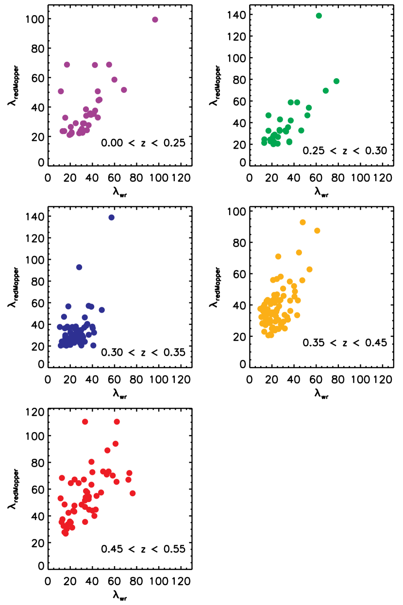
Figure 11: Comparison of the RedGOLD_wr richness ($\lambda_{wr}$) vs the redMaPPer richness ($\lambda_{redMaPPer}$) in different redshift bins as indicated in each panel.

We compare the two richness estimates in the 23 fields with deep $r$–band observations, and in Fig. 11 we plot the histogram of $\Delta\lambda/\lambda_{r}=(\lambda_{r}-\lambda_{wr})/\lambda_{r}$ in different redshift bins.

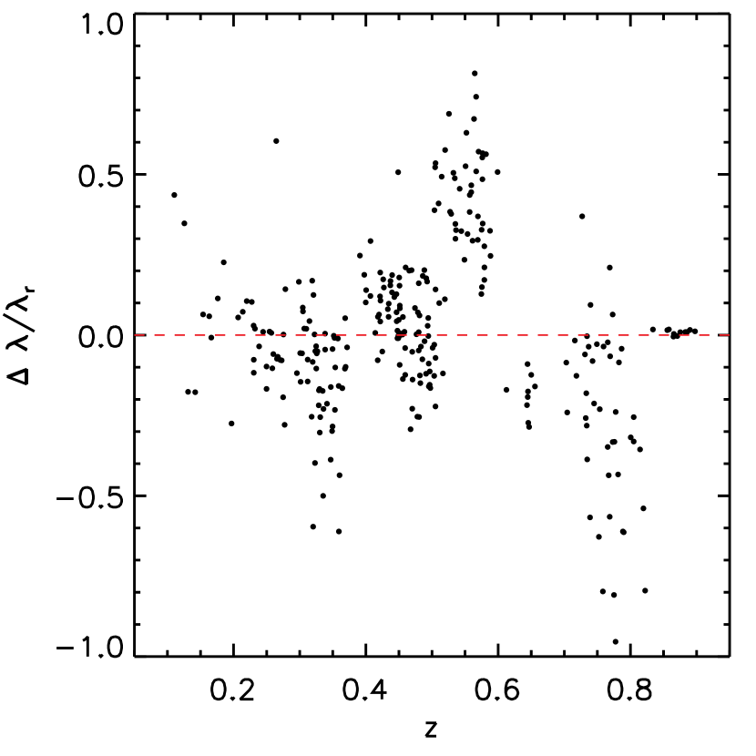
Figure 2: Comparison of the richness estimated using estimated using RedGOLD_r and RedGOLD_wr as a function of redshift. The red dashed line represents $(\lambda_{r}-\lambda_{wr})/\lambda_{r}=0$.

Fig. 2 shows $(\lambda_{r}-\lambda_{wr})/\lambda_{r}$ as a function of redshift. The red dashed line represents $(\lambda_{r}-\lambda_{wr})/\lambda_{r}=0$. Table 2 shows the median value of $(\lambda_{r}-\lambda_{wr})/\lambda_{r}$ and its standard deviation $\sigma_{\Delta\lambda}$ in redshift bins. At redshift $z<0.5$, the two richness estimates are in good agreement ($\Delta\lambda/\lambda_{r}<10\%$). In fact, the difference between the two measurements is not significant because when we use the color $(g-z)$ instead of $(g-r)$ to select red sequence galaxies, it still straddles the 4000 Å break. At $0.5<z<0.6$, the richness estimated without the $r$–band data is systematically underestimated by $\sim 40\%$ on average. This is because we use the $(g-i)$ color, which changes less steeply as a function of redshift than the $(r-i)$ and $(i-z)$ colors, and has larger photometric errors. At higher redshifts, $0.6<z<0.8$, we systematically over–estimate the optical richness estimated without the $r$–band by $\sim 20\%$, on average. In fact, when the r–data are unavailable, we only use the $(i-z)$ color constraint to identify red cluster members, while, when also using r–observations, we consider an additional cut in the $(r-z)$ color ($(r-i)$ at $z\sim 0.6$), which contributes to the reduction of the contamination of dusty red galaxies on the red-sequence. Finally, at $z>0.8$, the two richness estimates are in agreement because the $(i-z)$ color straddles the $4000$ Å break and it successfully isolates passive cluster members.

Since this comparison shows that at $z<0.5$ and $z\geq 0.8$, $\lambda_{wr}$ is on average under– or over–estimated by a factor $<10\%$, in this redshift range, we do not adopt a different richness threshold in the cluster catalog built using only four optical bands (hereafter, RedGOLD_wr) in these redshift intervals. However, at $0.5\leq z<0.8$, $\lambda_{wr}$ is on average significantly under– or overestimated (by a factor of $\sim 20-40\%$, depending on the redshift bin; see Table 2). This means that at $0.5<z<0.6$, we could discard real cluster candidates with $1\lesssim M_{200}\lesssim 2\times 10^{14}\ M_{\odot}$, and at $0.6\leq z<0.8$, we could include more false detections.

For this reason, in these redshift ranges, we apply different richness thresholds, estimated as $\lambda_{wr}\geq\lambda_{r,min}+\lambda_{r,min}\times median(\Delta\lambda)$, where $\lambda_{r,min}=10$ is the adopted optimized threshold when using the full band coverage. As we will discuss in section 5.3, this choice allows us to obtain both completeness and purity comparable with the cluster candidate catalog built using the full band coverage (hereafter, RedGOLD_r). The observed difference in richness should be carefully taken into account when studying scaling relations, such as the mass-richness, because it could introduce larger scatters.

5.2 Cluster catalog with deep $r$-band observations

In the $\sim 20\ \rm deg^{2}$ covered with deep $r$-band data, when (without) applying the thresholds on the RedGOLD parameters, we detect 294 (1045) cluster candidates, i.e. $\sim 15$ detections per square degree when applying the thresholds, in agreement with the values predicted for our cosmological model (Weinberg et al., 2013) in the same mass range. The $57\%$ ($31\%$) of the cluster candidates detected with (without) thresholds, have at least one SDSS spectroscopic member in less than $1.5^{\prime}$ with $|z_{spec}-z_{cluster}|<0.1$.

In the $\sim 20\ \rm deg^{2}$ covered by deep $r$-band observations, there are four X–ray detected clusters in the Piffaretti et al. (2011) catalog at redshift $0.05<z<0.25$. RedGOLD_r is able to recover three of them (either or not imposing the considered thresholds on the RedGOLD parameters), with masses included in the range $1.4\cdot 10^{14}\rm M_{\odot}<M_{500}<4.2\cdot 10^{14}\rm M_{\odot}$ and $0.08<z<0.2$. We miss one X–ray detection at $z=0.067$, with an estimated mass of $M_{500}=2.7\times 10^{13}\rm M_{\odot}$. This is not surprising, since we expect a completeness of $\lesssim 50\%$ in this mass and redshift range (L16).

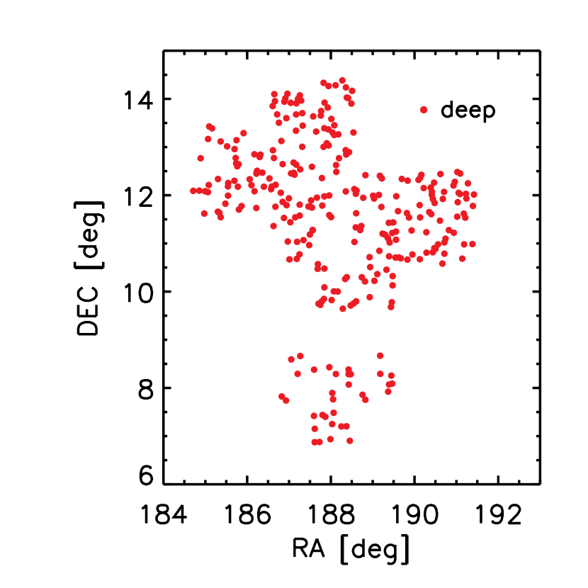
Figure 3: Spatial distribution of the NGVS cluster detections in the $\sim 20\ \rm deg^{2}$ covered by deep $r$-band observations. Red points represent detections in the fields with deep r–data, i.e. RedGOLD_r cluster candidates.

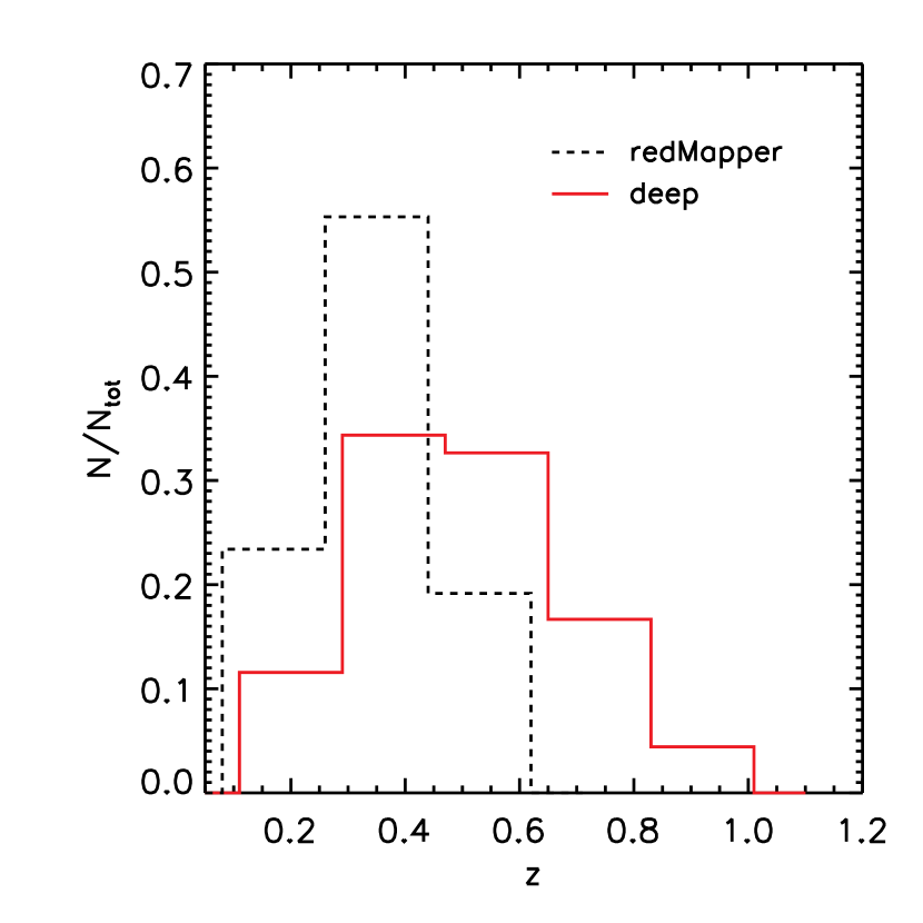
Figure 4: The redshift distribution of the RedGOLD_r cluster candidates (red solid line). The redMaPPer redshift distribution is shown by the black dashed line. Each histogram is normalized to the total number of detections.

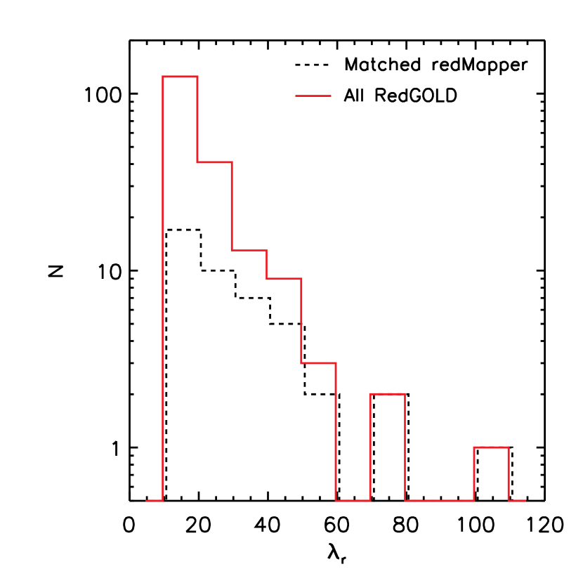
Figure 5: Richness distribution of the 294 RedGOLD_r cluster candidates (red solid) and of the RedGOLD candidates with a counterpart in the redMaPPer catalog (black dashed) in the $\sim 20\ \rm deg^{2}$ with deep $r$–band observations. Our catalog includes 150 detections (in the same area and redshift range, $z\leq 0.55$) that are not in the redMaPPer public catalog (see the text).

In Fig. 3, we show the spatial distribution of our detections in the fields covered by deep $r$–band observations as red points. In Fig. 4 and Fig. 5, we show their redshift and richness distribution (red solid line), respectively. For comparison, in Fig. 4 and Fig. 5, we plot the same distributions for the redMaPPer detections in the same area (black dashed line). The histograms are normalized to the corresponding total number of detections.

To match the RedGOLD cluster candidates with the redMaPPer catalog, we adopt the same matching algorithm described in L16, with a maximum projected distance between the centers corresponding to $R_{200}+\sigma_{R200}$ and a maximum redshift difference of $\Delta z=|z_{redMaPPer}-z_{RedGOLD}|\leq 3\times\sigma_{photoz}=3\times 0.03\times(1+z_{RedGOLD})$, where $z_{redMaPPer}$ is the cluster redshift in the redMaPPer catalog.

In the $\sim 20\ \rm deg^{2}$ covered by deep $r$–band observations, RedGOLD_r recovers all the 53 redMaPPer clusters, without limits on $\sigma_{det}$, $\lambda$, and the cluster radial profile. When applying limits in $\sigma_{det}$, $\lambda$ and the cluster radial profile, we obtain 46 clusters, for a recovery of $87^{+4}_{-6}\%$/$100\%$, when using/not using the thresholds. The seven detections that are discarded when using the thresholds have significance levels below our adopted threshold in $\sigma_{det}$, and/or richness $\lambda_{r}<10$.

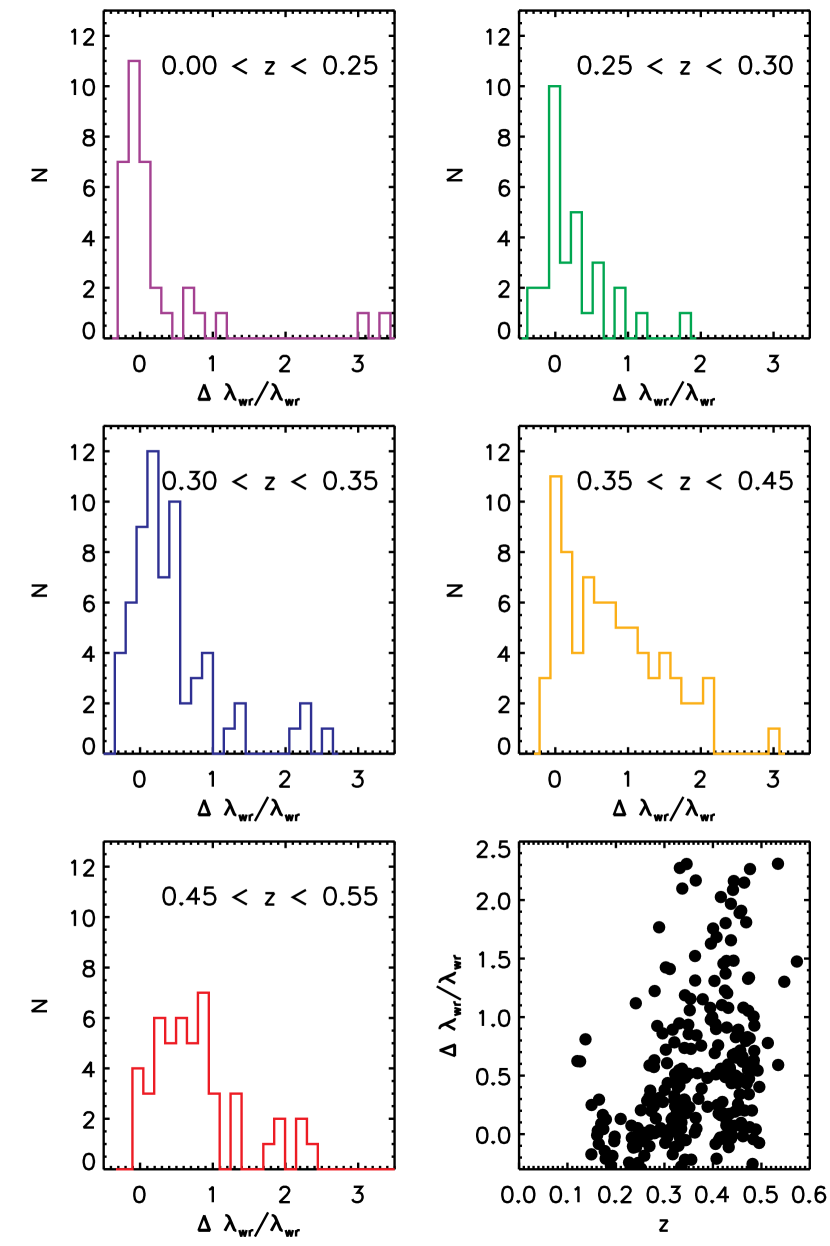
Figure 12: Histogram of $\frac{\Delta\lambda_{wr}}{\lambda_{wr}}=\frac{\lambda_{redMaPPer}-\lambda_{wr}}{\lambda_{wr}}$, in different redshift bins as indicated in each panel. The bottom right panel shows the $\frac{\Delta\lambda_{wr}}{\lambda_{wr}}$ distribution as a function of redshift $z$.

In Fig. 11 and Fig 12, we compare the richness estimates obtained by redMaPPer and RedGOLD for the 46 common detections. We show $\lambda_{r}$ vs $\lambda_{redMaPPer}$ and the histogram of the difference between our richness definition and the richness adopted in Rykoff et al. (2014). Different colors show the observed difference in different redshift bins, as indicated in each panel. In the bottom right panel in Fig. 12, we plot the ($\lambda_{redMaPPer}-\lambda_{r})/\lambda_{r}$ as a function of redshift: as already shown in L16, the difference between the two richness estimates in the RedGOLD and redMaPPer catalog is larger at higher redshift. We have shown that for our CFHT-LS W1 RedGOLD cluster candidate sample, the redMaPPer richness is systematically higher than the RedGOLD richness at $z>0.3$, and Table 4 of that work gives the median ($\lambda_{redMaPPer}-\lambda_{r})/\lambda_{r}$ in five different redshift bins. For this work, in the $\sim 20\ \rm deg^{2}$ covered by deep $r$–band observations, we do not have enough statistics to obtain solid median difference estimates as in L16. In Table 3, we present the median value of this richness difference as a function of redshift. These results are consistent with Table 4 in L16 and show that the median difference is small at low redshift ($z<0.3$), but increases at higher redshifts. The first bin has few detections and it is not statistically significant.

The RedGOLD_r catalog includes 150 new detections with respect to the redMaPPer catalog in the same area and the redshift range covered by the redMaPPer catalog ($z\leq 0.55$). We extensively discussed the comparison between RedGOLD_r–like and redMaPPer detection in section 6.3 in L16, where we concluded that because of the richness limit imposed to the redMaPPer catalog (Rozo, private communication) and the greater depth of the NGVS compared to the SDSS, RedGOLD_r detects cluster candidates at lower mass and higher redshift than those in the redMaPPer published catalog (as it is shown in Fig. 4 and Fig. 5). A more detailed comparison of the two detection algorithms should be done on exactly the same photometric and photometric redshift catalogs on the same area, and this is a good subject for future work.

5.3 Cluster catalog with four bandpasses

To build a homogenous selection on the whole NGVS area, we also provide a cluster catalog using only four bandpasses, adopting the same approach described in the case of the fields covered by deep $r$-band observations, but isolating red-sequence galaxies using different color pairs, as described in section 5 and using a corrected $\lambda_{wr}$ limit, as explained in section 5.1.

When (without) applying the thresholds on the RedGOLD parameters, RedGOLD_wr finds 1724 (6233) cluster candidates up to $z=1.1$, i.e. $\sim 15$ detections per square degree when applying the thresholds. The $\sim 62\%$ ($\sim 36\%$) of the cluster candidates detected with (without) the thresholds have at least one SDSS spectroscopic member in less than $1.5^{\prime}$ with $|z_{spec}-z_{cluster}|<0.1$.

To quantify the completeness and the purity of the RedGOLD_wr catalog and compare it with RedGOLD_r, we apply RedGOLD_wr to $\sim 3\ \rm deg^{2}$ in the CFHT-LS W1 field, covered by the X–ray detected cluster catalog by Gozaliasl et al. (2014), which includes 135 clusters and groups (hereafter, the CFHT-LS W1 GZ field).

As discussed in L16, in the CFHT-LS W1 GZ field, RedGOLD_r finds 38 cluster candidates up to $z\sim 1$ and 28 of them have an X–ray counterpart in Gozaliasl et al. (2014). Among the Gozaliasl et al. (2014) clusters with $M_{200}>10^{14}\ \rm M_{\odot}$, RedGOLD_r recovers 100% of them up to $z=0.5$ and $76^{+11}_{-15}\%$ in the whole redshift range. In the same area, RedGOLD_wr finds 42 cluster candidates up to $z\sim 1$, of which 33 are in common with Gozaliasl et al. (2014) and 30 are also detected by RedGOLD_r. Among the Gozaliasl et al. (2014) clusters with $M_{200}>10^{14}\ \rm M_{\odot}$, RedGOLD_wr recovers all of them up to $z=0.5$ and $71^{+12}_{-15}\%$ in the whole redshift range. Two cluster candidates detected by RedGOLD_wr and without an X–ray counterpart have been spectroscopically confirmed as clusters at $z=0.33$ (Andreon et al., 2004) and $z=0.92$ (Pierre et al., 2006, C3 cluster). This implies that the lower limit on the purity with RedGOLD_wr is of $\sim 80\%$.

This means that, when adopting different thresholds of $\lambda$ as a function of redshift according to the median values reported in Table 2, we obtain similar values of completeness and purity with RedGOLD_r and RedGOLD_wr.

To directly compare the RedGOLD_wr and RedGOLD_r catalogs, we also checked the detections that are not found in both cases.

Eight RedGOLD_r candidates are not detected by RedGOLD_wr: two are discarded when performing the fit of the color-magnitude relation, four because they have $\sigma_{det}<4$, one because of the galaxy distribution constraint, and one when imposing our lower limit on the richness. Twelve RedGOLD_wr cluster candidates are not detected with RedGOLD_r. Six of them have an X–ray counterpart in the group catalog by (Gozaliasl et al., 2014, $M\leq 8.5\times 10^{13}\ \rm M_{\odot}$) and one is a spectroscopically confirmed system at $z=0.92$ Pierre et al. (2006). The remaining five RedGOLD_wr detections are detected as red–overdensities also by RedGOLD_r, but they are discarded because of the imposed constraints: in particular, one is discarded when performing the fit of the CMR, two are discarded because of our constraints on the NFW profile, one because of its detection significance ($\sigma_{det}<4.5$) and one because of its richness estimate $\lambda_{r}$.

These results suggest that the additional cluster candidates detected by RedGOLD_wr and unrecovered by RedGOLD_r correspond to less massive systems.

To summarize, the lack of the $r$–band seems to have a minor effect on the RedGOLD completeness and does not impact its purity. With RedGOLD_wr, we miss only $\sim 5\%$ of the RedGOLD_r detections more massive than $10^{14}\ \rm M_{\odot}$ at higher redshift (z>0.5), while we obtain the same completeness of $100\%$ at lower redshift.

In Fig. 8, we show the spatial distribution of the RedGOLD_wr detections. In Fig. 9, we show their redshift distribution (solid line).

For comparison, in Fig. 9, we show the redMaPPer detections (dashed line) in the same area. Up to $z\sim 0.55$, we find that RedGOLD_wr recovers all the 267 redMaPPer candidates. When applying limits in $\sigma_{det}$, $\lambda$ and the cluster radial profile, we obtain 238 detections, for a final recovery of $90^{+2}_{-2}\%$/$100\%$ with/without thresholds in the RedGOLD parameters.

In Fig. 10, we compare the richness distribution of the RedGOLD_wr cluster candidates (solid line) with respect to the richness of the redMaPPer detections recovered by RedGOLD_wr (dashed line). In the RedGOLD_wr catalog, we detect 1032 new cluster candidates in the same area and redshift range of the redMaPPer catalog ($z\leq 0.55$), which are distributed at lower richness with respect to the redMaPPer catalog (i.e. $\sim 10$ new cluster candidate per $\rm deg^{2}$ up to $z\sim 0.55$), because of both the richness threshold adopted in the redMaPPer catalog (Rozo, private communication) and the higher depth of the NGVS with respect to the SDSS data.

In Fig. 11 and Fig 12 we compare the richness estimates obtained by redMaPPer and RedGOLD for the 238 common detections. We show the $\lambda_{wr}$ vs $\lambda_{redMaPPer}$ and the histogram of the difference between our richness definition and the richness adopted in Rykoff et al. (2014). Different colors show the observed difference in different redshift bins, as indicated in each panel. Consistently with our results in L16, the redMaPPer richness is systematically higher than the RedGOLD richness at $z>0.3$. In the bottom right panel in Fig. 12, we plot the ($\lambda_{redMaPPer}-\lambda_{wr})/\lambda_{wr}$ as a function of redshift: as already shown in L16, the difference between the two richness estimates in the RedGOLD and redMaPPer catalog is larger at higher redshift. In Table 4, we present the median value of this richness difference as a function of redshift. The median difference is small at low redshift ($z<0.3$), but it increases at higher redshifts.

These results are consistent with our results in the fields covered by five bands (Table 3) and L16, within the errors. As discussed in L16, we believe that this difference might be due to the fact that we keep a simple approach counting galaxies up to the depth reached by the CFHTLenS, while the redMaPPer richness estimate includes an extrapolation of the SDSS depth (which is lower than CFHTLenS) to our same limit in ${\rm L^{*}}$. It would be worth investigating the observed difference richness in a future work in collaboration with the redMapper authors, considering a larger cluster sample and using the same photometric and photometric redshift catalogs.

Finally, we compare the RedGOLD_wr detections with the nine X–ray cluster catalog by Piffaretti et al. (2011): we find that RedGOLD_wr is able to recover seven of them without imposing constraints on the $\sigma_{det}$, $\lambda$ and the cluster radial profile, in the range $1.3\cdot 10^{14}\rm M_{\odot}<M_{500}<4.3\cdot 10^{14}\rm M_{\odot}$ and $0.08<z<0.55$. Three of them are also detected by RedGOLD_r. The other two clusters have masses of $M_{500}=3-5\cdot 10^{13}$ (they are low mass systems) and $z=0.04-0.09$. When considering our lower limits on the RedGOLD parameters, we discard two of the detected clusters because of their $\sigma_{det}$ or the radial galaxy distribution. The clusters that are discarded while imposing limits have masses $M_{500}\sim 1.4\cdot 10^{14}\ \rm M_{\odot}$ and $z\sim 0.08$.

5.4 The NGVS Cluster Candidate Catalogs

The NGVS RedGOLD cluster candidate catalogs, obtained with the thresholds on the RedGOLD parameters, will be public when this paper is published. We provide two independent catalogs: one for the $\sim 20\ \rm deg^{2}$ with deep $r$–band observations, and the other for the whole NGVS area, using only four optical bands.

In our catalogs, we include the following parameters for each RedGOLD detection:

1. the J2000 right ascension RA

2. the J2000 declination decl.

3. the photometric cluster redshift PHOTZ

4. the error in photometric redshift ePHOTOZ

5. the average spectroscopic redshift, when available SPECZ

6. the detection significance $\sigma_{det}$ SDET

7. the cluster richness $\lambda$ RICH

8. the uncertainty on cluster richness $\lambda_{err}$ eRICH

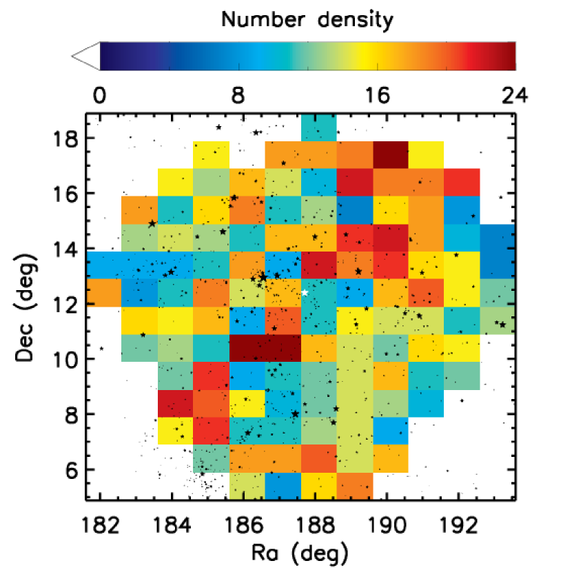
Figure 13: Density plot of the RedGOLD detections in each MegaCam pointing. Different colors correspond to different number of cluster candidates per MegaCam field using four bandpasses, as shown in the color bar. There is no correlation between the number of detected candidates and the position of the Virgo cluster members. In fact, Virgo bright members mask NGVS areas in which we cannot detect clusters, however this bias is within the variations in the number of detections from pointing to pointing (see text).

Virgo galaxies and globular clusters are excluded from our sample by the photometric and photometric redshift selection, as shown in Raichoor et al. (2014). However, the NGVLens reduction includes masking areas for which holes and the noise due to bright Virgo galaxies would prevent background galaxy detection. This means that, to have a homogeneous photometry and photometric redshift catalog, we do not detect clusters in the masked areas. To quantify how this biases our catalogs, in Fig. 13 we show the density distribution of our detections in each MegaCam field using four bandpasses. Different colors correspond to the different number of cluster candidates per MegaCam pointing, as shown in the color bar, and the black stars represent the Virgo cluster members from Kim et al. (2014). The symbol size is proportional to the corresponding Kron radius from Kim et al. (2014). The white star represents M87.

When using four bandpasses, the average number of clusters per square degree is $15\pm 4$ (the uncertainty is the standard deviation of the distribution of detection for each pointing), consistent with our detections in the CFHT-LS W1(L16). We obtain a corrected $19\pm 6$ when the number of detected clusters in each MegaCam pointing is divided by the unmasked area in that pointing. In Fig. 13, density variations in different pointings are all consistent within $\sim 2\sigma$, independently on the masks due to the presence of stars and Virgo galaxies. Also, when we perform a Pearson, Spearman and Kendall correlation test on the number of detection vs the masked area, we obtain a probability of $42-45\%$ that the two variables are not correlated. This means that statistical variations in the cluster detection distribution are more significant than the correlation between the number of detected clusters and the masked area (e.g. the presence of stars and Virgo galaxies). We deduce that the presence of bright Virgo galaxies prevent us from detecting clusters in the masked areas, and, from the percentage of masked area and assuming that the cluster distribution is the same in the masked and unmasked area, we estimate that $\sim 20\%$ of the clusters will be missed. However, as shown in L16, this does not significantly bias our detections in the unmasked area. We have already discussed in Sec. 5.3 that the lack of the r-band biases our richness estimates. This should be taken into account when using these catalogs for cosmology and other predictions based on the number of detected clusters.

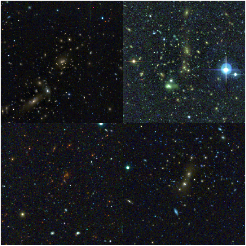
Figure 14: Optical images of four cluster candidates detected by RedGOLD in the NGVS area at redshift $z_{cluster}=0.16$ (left upper panel), $z_{cluster}=0.27$ (right upper panel), $z_{cluster}=0.48$ (left lower panel) and $z_{cluster}=0.25$ (right lower panel). Their detection significance and richness are $\sigma_{det}=7.7,\lambda=96.6$, $\sigma_{det}=10.3,\lambda=78.3$, $\sigma_{det}=19.4,\lambda=76.3$ and $\sigma_{det}=10.4,\lambda=68.5$.

In Fig. 14 we show the optical images of four RedGOLD detections in the NGVS field.

6 Conclusions

We apply our cluster detection algorithm RedGOLD (L16) to deep optical observations from the NGVS (Ferrarese et al., 2012), which covers $104\ \rm deg^{2}$ around the center of the Virgo cluster.

RedGOLD is a cluster detection algorithm based on the selection of passive galaxy overdensities, simultaneously using two pairs of filters, corresponding to the $(U-B)$ and $(B-V)$ rest–frame colors (L16). It also imposes constraints on the detections to be compatible with an NFW profile. For each cluster candidate, it estimates the detection significance $\sigma_{det}$, and provides a richness measurement $\lambda$ based on the number of luminous red–sequence galaxies. In L16, we showed that, at the NGVS depth, the best compromise between purity and completeness is reached for detections with richness $\lambda\geq 10$ and detection significance $\sigma_{det}\geq 4\ (\geq 4.5)$ at $z\leq 0.6$ ($z\lesssim 1$), according to both empirical calibration on the X–ray group catalog by Gozaliasl et al. (2014) and simulations (Springel et al., 2005; Guo et al., 2011; Henriques et al., 2012). With these limits, we expect our cluster candidate catalogs to be $\sim 100\%$($\sim 70\%$) complete and $\sim 80\%$ pure, at $z\leq 0.6$($z\lesssim 1$), for galaxy clusters with masses $M\gtrsim 10^{14}\ M_{\odot}$. Our cluster centering algorithm attains a median separation between the peak of the X–ray emission and our RedGOLD cluster centers of $17.2^{\prime\prime}\pm 11.2^{\prime\prime}$, and our determination of the cluster photometric redshifts differ from spectroscopic redshifts by less than 0.05 up to $z\sim 1$ (L16).

Part of the NGVS area, $\sim 20\ \rm deg^{2}$, has been observed in five bandpasses ($u^{*},g,r,i,z$) to the nominal NGVS depth (Ferrarese et al., 2012; Raichoor et al., 2014). Over the remaining survey area, the $r$–band is either shallower ($\sim 10\ \rm deg^{2}$; see Table 1), or has not been observed ($\sim 74\ \rm deg^{2}$). In these fields, the photometric redshift estimates are less accurate (Raichoor et al., 2014), especially in the redshift range of $0.3<z<0.8$, since the missing $r$–band is one of the two bands that straddles the $4000$ Å break.

Because of this difference in the $r$–band coverage, we build two independent RedGOLD cluster catalogs: one using the deep $r$–band observations, available only over $\sim 20\ \rm deg^{2}$ (the RedGOLD_r catalog), and the other using only four bandpasses over the entire NGVS area (the RedGOLD_wr catalog).

We show that the lack of the $r$–band observations impacts the estimation of the cluster richness $\lambda$. To estimate the corresponding bias, we use the $\sim 20\ \rm deg^{2}$ covered by deep $r$–band data and compare the two cluster richness estimates obtained with five and four bandpasses, i.e., with RedGOLD_r and RedGOLD_wr, respectively. We find that the lack of the $r$–band observations does not affect the cluster richness estimate up to $z\sim 0.5$ and at $z>0.8$. At $0.5\leq z<0.6$, the cluster richness estimated without using the $r$–band is underestimated by a factor of $\sim 40\%$, while at $0.6\leq z<0.8$ it is systematically overestimated by a factor of $\sim 20\%$. As a consequence, we adopt different lower limits on $\lambda$ when applying RedGOLD_wr at these redshifts, taking into account the median estimated difference $\lambda_{r}-\lambda_{wr}$. With this choice, using the X–ray group catalog by Gozaliasl et al. (2014), we demonstrate that RedGOLD_r reaches similar completeness and purity as RedGOLD_wr.

Over the $\sim 20\ \rm deg^{2}$ with complete and deep r–band coverage, we find 294 (1045) cluster candidates up to $z\sim 1$, i.e. $\sim 15$ detections per $\rm deg^{2}$, when applying (not applying) the threshold on RedGOLD parameters. Of the cluster candidates detected with (without) considering lower limits on the cluster richness, the detection significance or the cluster radial distribution, $57\%$ ($31\%$) have at least one SDSS spectroscopic member in less than $1.5^{\prime}$ with $|z_{spec}-z_{cluster}|<0.1$.

When using four optical bands, we find 1724 (6233) cluster candidates up to $z\sim 1$ over the entire NGVS area, i.e. $\sim 15$ detections per $\rm deg^{2}$, when applying (not applying) the threshold on RedGOLD parameters. Of the cluster candidates detected with (without) considering lower limits on the cluster richness, the detection significance or the cluster radial distribution, $62\%$ ($36\%$) have at least one SDSS spectroscopic member in less than $1.5^{\prime}$ with $|z_{spec}-z_{cluster}|<0.1$.

With RedGOLD_wr, we recover most of the X–ray detected clusters with $M_{500}>1.4\times 10^{14}\rm M_{\odot}$ and $0.08<z<0.2$. RedGOLD recovers all of the redMaPPer detections (Rykoff et al., 2014) in all fields when we do not apply the thresholds on RedGOLD parameters. When we do apply our thresholds on the RedGOLD parameters, we find $90\%$ of redMaPPer detections over the deep $r$–band data area, and $87\%$ of redMaPPer detections over the entire NGVS area in which we used only four bands.

These results confirm that RedGOLD successfully detects galaxy clusters, and show that even when using only four optical bands, RedGOLD is able to provide cluster catalogs with high completeness and purity, as shown in L16.

The NGVS cluster candidate catalogs will be made public on the NGVS website once this paper appears in publication.

Figure 1: Comparison of the richness estimated using RedGOLD_r (the algorithm is run using the full band coverage, five bands) and RedGOLD_wr (the algorithm is run without using the $r$–band), in the $23\ \rm deg^{2}$ covered by deep $r$–band observations. Each panel shows the distribution of $(\lambda_{r}-\lambda_{wr})/\lambda_{r}$ in different redshift bins, where $\lambda_{wr}$ is the richness estimated without using the $r$–band and $\lambda_{r}$ is the richness estimated using the deep r–band data, which we are assuming to be our reference cluster richness.

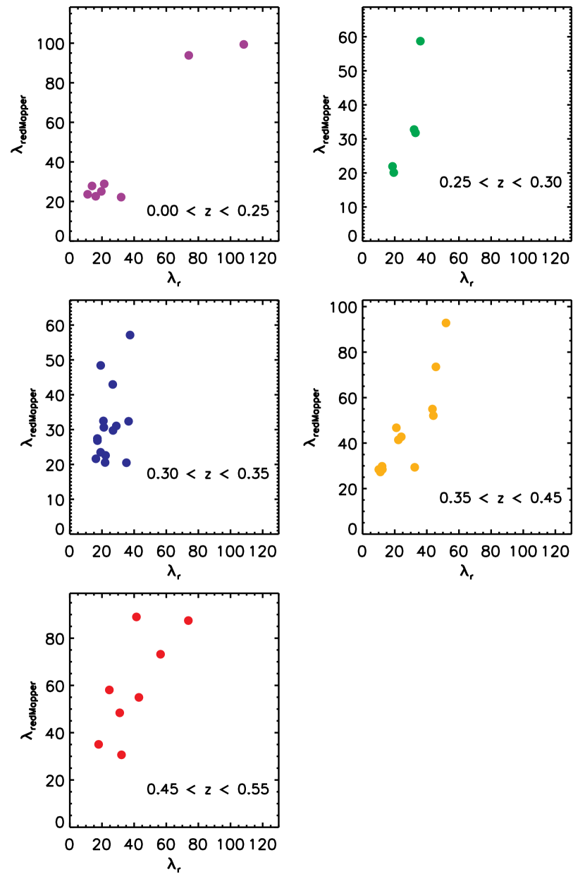
Figure 6: Comparison of the RedGOLD_r richness ($\lambda_{r}$) vs the redMaPPer richness ($\lambda_{redMaPPer}$) in different redshift bins as indicated in each panel.

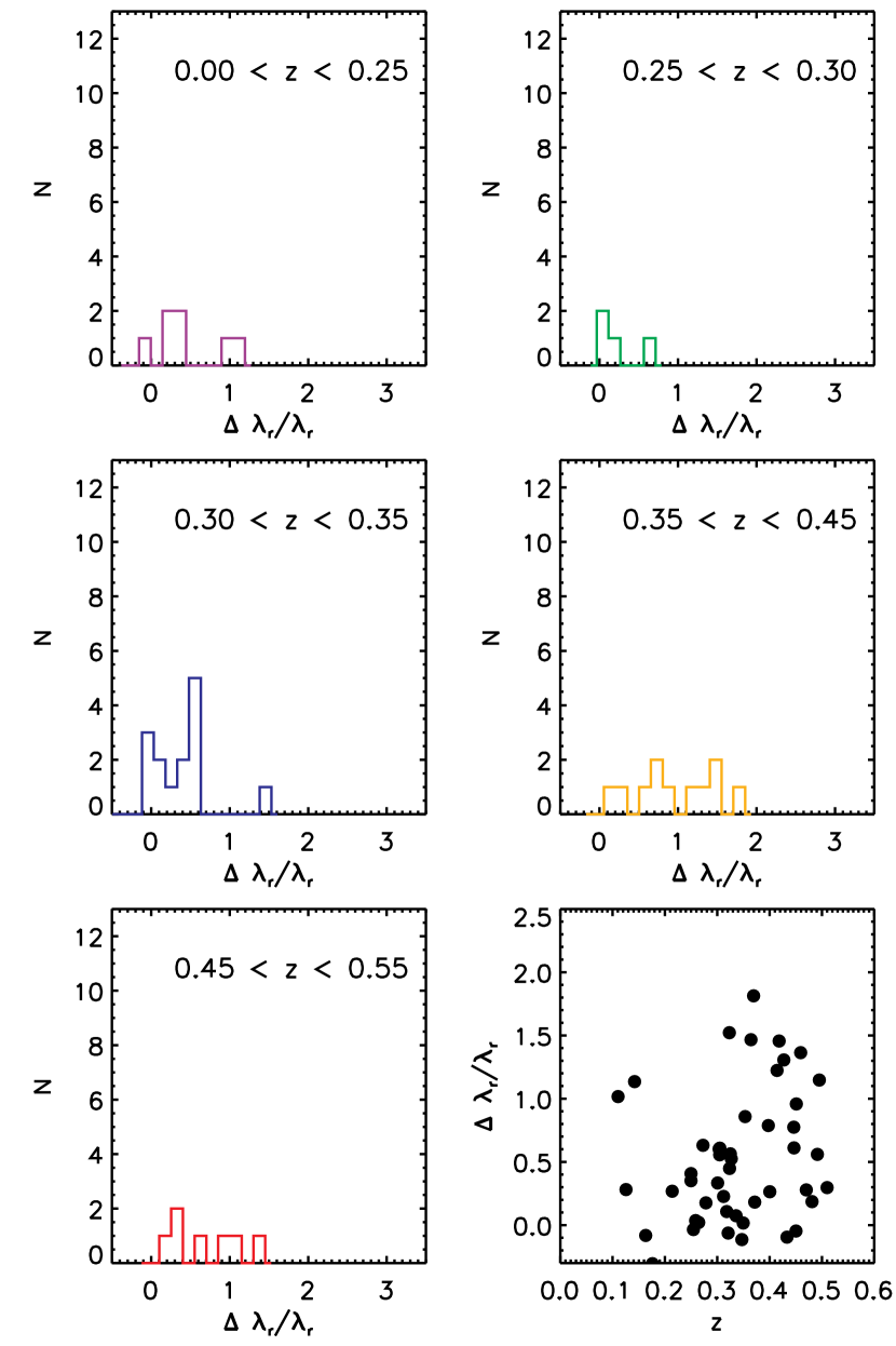
Figure 7: Histogram of $\frac{\Delta\lambda_{r}}{\lambda_{r}}=\frac{\lambda_{redMaPPer}-\lambda_{r}}{\lambda_{r}}$, in different redshift bins as indicated in each panel. The bottom right panel shows the $\frac{\Delta\lambda_{r}}{\lambda_{r}}$ distribution as a function of redshift $z$.

Figure 8: Spatial distribution of the NGVS cluster candidates in the $104\ \rm deg^{2}$, detected using four optical bands.

Figure 9: Redshift distribution of the RedGOLD_wr cluster candidates (i.e., detected using four optical bands in the entire NGVS field) (solid line). The dashed line represents the redMaPPer detections. Each histogram is normalized to the total number of detections.

Figure 10: Richness distribution of the RedGOLD_wr cluster candidates (solid line) and of the RedGOLD_wr candidates with a counterpart in the redMaPPer catalog (dashed line). Our catalog includes detections with lower richness, i.e. it reaches a lower mass limit with respect to the redMaPPer catalog.

Table 1: NGVS exposure times, magnitude limits and average seeings in the five optical bands. As the $r$-band data show a large field-to-field depth variation, we provide the magnitude limits range spanned in the different fields (from Table 1, Raichoor et al., 2014). $mag_{lim}$ is the 5$\sigma$ detection limit in a 2″aperture (see the details of the estimation in Raichoor et al., 2014).

Filter	exposure time [s]	$mag_{lim}$ [AB]	seeing [”]
u*	6402	$25.60\pm 0.16$	$0.83\pm 0.07$
g	3230	$25.73\pm 0.13$	$0.77\pm 0.08$
r	1374	$[23.56,25.51]$	$0.74\pm 0.14$
i	2055	$24.41\pm 0.13$	$0.52\pm 0.04$
z	4466	$23.62\pm 0.16$	$0.70\pm 0.08$

Table 2: Median value of the difference $(\lambda_{r}-\lambda_{wr})/\lambda_{r}$ and its standard deviation.

redshift	$median(\Delta\lambda/\lambda_{r})$	$\sigma_{\Delta\lambda}$
$0.1\leq z<0.2$	0.06	0.24
$0.2\leq z<0.3$	-0.04	0.11
$0.3\leq z<0.4$	-0.08	0.17
$0.4\leq z<0.5$	0.05	0.14
$0.5\leq z<0.6$	0.38	0.23
$0.6\leq z<0.7$	-0.18	0.07
$0.7\leq z<0.8$	-0.24	0.33
$0.8\leq z<1.1$	0.01	0.01

redshift	median($\Delta\lambda_{r}/\lambda_{r}$)
$z\leq 0.25$	0.4 $\pm$ 0.5
$0.25<z\leq 0.30$	0.0 $\pm$ 0.3
$0.30<z\leq 0.35$	0.3$\pm$ 0.5
$0.35<z\leq 0.45$	0.9 $\pm$ 0.6
$0.45<z\leq 0.55$	0.6 $\pm$ 0.5

Table 3: Median value of $(\lambda_{redMaPPer}-\lambda_{r})/\lambda_{r}$ in different redshift bins, obtained using a 3 $\sigma$ clipping.

redshift	median($\Delta\lambda_{wr}/\lambda_{wr}$)
$z\leq 0.25$	0.0 $\pm$ 0.8
$0.25<z\leq 0.30$	0.1 $\pm$ 0.5
$0.30<z\leq 0.35$	0.3$\pm$ 0.6
$0.35<z\leq 0.45$	0.7 $\pm$ 0.7
$0.45<z\leq 0.55$	0.7 $\pm$ 0.9

Table 4: Median value of $(\lambda_{redMaPPer}-\lambda_{wr})/\lambda_{wr}$ in different redshift bins, obtained using a 3 $\sigma$ clipping.

References

- Andreon et al. (2004) Andreon, S., Willis, J., Quintana, H., et al. 2004, MNRAS, 353, 353
- Arnouts et al. (1999) Arnouts, S., Cristiani, S., Moscardini, L., et al. 1999, MNRAS, 310, 540
- Arnouts et al. (2002) Arnouts, S., Moscardini, L., Vanzella, E., et al. 2002, MNRAS, 329, 355
- Bellagamba et al. (2011) Bellagamba, F., Maturi, M., Hamana, T., et al. 2011, MNRAS, 413, 1145
- Benítez (2000) Benítez, N. 2000, ApJ, 536, 571
- Benítez et al. (2004) Benítez, N., Ford, H., Bouwens, R., et al. 2004, ApJS, 150, 1
- Bertin & Arnouts (1996) Bertin, E., & Arnouts, S. 1996, A&AS, 117, 393
- Boulade et al. (2003) Boulade, O., Charlot, X., Abbon, P., et al. 2003, in Society of Photo-Optical Instrumentation Engineers (SPIE) Conference Series, Vol. 4841, Instrument Design and Performance for Optical/Infrared Ground-based Telescopes, ed. M. Iye & A. F. M. Moorwood, 72–81
- Brodwin et al. (2013) Brodwin, M., Stanford, S. A., Gonzalez, A. H., et al. 2013, ApJ, 779, 138
- Bruzual & Charlot (2003) Bruzual, G., & Charlot, S. 2003, MNRAS, 344, 1000
- Capak et al. (2004) Capak, P., Cowie, L. L., Hu, E. M., et al. 2004, AJ, 127, 180
- Chiang et al. (2013) Chiang, Y.-K., Overzier, R., & Gebhardt, K. 2013, ApJ, 779, 127
- Coe et al. (2006) Coe, D., Benítez, N., Sánchez, S. F., et al. 2006, AJ, 132, 926
- Coleman et al. (1980) Coleman, G. D., Wu, C.-C., & Weedman, D. W. 1980, ApJS, 43, 393
- Cooper et al. (2008) Cooper, M. C., Newman, J. A., Weiner, B. J., et al. 2008, MNRAS, 383, 1058
- Dawson et al. (2013) Dawson, K. S., Schlegel, D. J., Ahn, C. P., et al. 2013, AJ, 145, 10
- Ebeling & Wiedenmann (1993) Ebeling, H., & Wiedenmann, G. 1993, Phys. Rev. E, 47, 704
- Eisenstein et al. (2001) Eisenstein, D. J., Annis, J., Gunn, J. E., et al. 2001, AJ, 122, 2267
- Erben et al. (2013) Erben, T., Hildebrandt, H., Miller, L., et al. 2013, MNRAS, 433, 2545
- Evrard et al. (2008) Evrard, A. E., Bialek, J., Busha, M., et al. 2008, ApJ, 672, 122
- Ferrarese et al. (2012) Ferrarese, L., Côté, P., Cuillandre, J.-C., et al. 2012, ApJS, 200, 4
- Finoguenov et al. (2003) Finoguenov, A., Borgani, S., Tornatore, L., & Böhringer, H. 2003, A&A, 398, L35
- Finoguenov et al. (2009) Finoguenov, A., Connelly, J. L., Parker, L. C., et al. 2009, ApJ, 704, 564
- George et al. (2011) George, M. R., Leauthaud, A., Bundy, K., et al. 2011, ApJ, 742, 125
- George et al. (2012) —. 2012, ApJ, 757, 2
- Gillis et al. (2013) Gillis, B. R., Hudson, M. J., Erben, T., et al. 2013, MNRAS, 431, 1439
- Gladders & Yee (2000) Gladders, M. D., & Yee, H. K. C. 2000, AJ, 120, 2148
- Gozaliasl et al. (2014) Gozaliasl, G., Finoguenov, A., Khosroshahi, H. G., et al. 2014, A&A, 566, A140
- Grove et al. (2009) Grove, L. F., Benoist, C., & Martel, F. 2009, A&A, 494, 845
- Guo et al. (2011) Guo, Q., White, S., Boylan-Kolchin, M., et al. 2011, MNRAS, 413, 101
- Gwyn (2012) Gwyn, S. D. J. 2012, ApJ, 143, 38
- Henriques et al. (2012) Henriques, B. M. B., White, S. D. M., Lemson, G., et al. 2012, MNRAS, 421, 2904
- Hildebrandt et al. (2012) Hildebrandt, H., Erben, T., Kuijken, K., et al. 2012, MNRAS, 421, 2355
- Ilbert et al. (2006) Ilbert, O., Arnouts, S., McCracken, H. J., et al. 2006, A&A, 457, 841
- Johnston et al. (2007) Johnston, D. E., Sheldon, E. S., Wechsler, R. H., et al. 2007, ArXiv e-prints, arXiv:0709.1159
- Kaiser et al. (2002) Kaiser, N., Aussel, H., Burke, B. E., et al. 2002, in Society of Photo-Optical Instrumentation Engineers (SPIE) Conference Series, Vol. 4836, Survey and Other Telescope Technologies and Discoveries, ed. J. A. Tyson & S. Wolff, 154–164
- Kim et al. (2014) Kim, S., Rey, S.-C., Jerjen, H., et al. 2014, ApJS, 215, 22
- Kinney et al. (1996) Kinney, A. L., Calzetti, D., Bohlin, R. C., et al. 1996, ApJ, 467, 38
- Larson & Tinsley (1978) Larson, R. B., & Tinsley, B. M. 1978, ApJ, 219, 46
- Laureijs et al. (2011) Laureijs, R., Amiaux, J., Arduini, S., et al. 2011, ArXiv e-prints, arXiv:1110.3193
- Le Fèvre et al. (2013) Le Fèvre, O., Cassata, P., Cucciati, O., et al. 2013, A&A, 559, A14
- Licitra et al. (2016) Licitra, R., Mei, S., Raichoor, A., Erben, T., & Hildebrandt, H. 2016, MNRAS, 455, 3020
- Lin et al. (2004) Lin, Y.-T., Mohr, J. J., & Stanford, S. A. 2004, ApJ, 610, 745
- LSST Dark Energy Science Collaboration (2012) LSST Dark Energy Science Collaboration. 2012, ArXiv e-prints, arXiv:1211.0310
- McGee et al. (2009) McGee, S. L., Balogh, M. L., Bower, R. G., Font, A. S., & McCarthy, I. G. 2009, MNRAS, 400, 937
- Mead et al. (2010) Mead, J. M. G., King, L. J., Sijacki, D., et al. 2010, MNRAS, 406, 434
- Mehrtens et al. (2012) Mehrtens, N., Romer, A. K., Hilton, M., et al. 2012, MNRAS, 423, 1024
- Mei et al. (2009) Mei, S., Holden, B. P., Blakeslee, J. P., et al. 2009, ApJ, 690, 42
- Mei et al. (2015) Mei, S., Scarlata, C., Pentericci, L., et al. 2015, ApJ, 804, 117
- Milkeraitis et al. (2010) Milkeraitis, M., van Waerbeke, L., Heymans, C., et al. 2010, MNRAS, 406, 673
- Muzzin et al. (2013) Muzzin, A., Wilson, G., Demarco, R., et al. 2013, ApJ, 767, 39
- Navarro et al. (1996) Navarro, J. F., Frenk, C. S., & White, S. D. M. 1996, ApJ, 462, 563
- Oke & Gunn (1983) Oke, J. B., & Gunn, J. E. 1983, ApJ, 266, 713
- Olsen et al. (2007) Olsen, L. F., Benoist, C., Cappi, A., et al. 2007, A&A, 461, 81
- Paudel et al. (2013) Paudel, S., Duc, P.-A., Côté, P., et al. 2013, ApJ, 767, 133
- Pierre et al. (2006) Pierre, M., Pacaud, F., Duc, P.-A., et al. 2006, MNRAS, 372, 591
- Piffaretti et al. (2011) Piffaretti, R., Arnaud, M., Pratt, G. W., Pointecouteau, E., & Melin, J.-B. 2011, A&A, 534, A109
- Prevot et al. (1984) Prevot, M. L., Lequeux, J., Prevot, L., Maurice, E., & Rocca-Volmerange, B. 1984, A&A, 132, 389
- Raichoor et al. (2014) Raichoor, A., Mei, S., Erben, T., et al. 2014, ApJ, 797, 102
- Rozo et al. (2011) Rozo, E., Rykoff, E., Koester, B., et al. 2011, ApJ, 740, 53
- Rykoff et al. (2014) Rykoff, E. S., Rozo, E., Busha, M. T., et al. 2014, ApJ, 785, 104
- Shankar et al. (2013) Shankar, F., Marulli, F., Bernardi, M., et al. 2013, MNRAS, 428, 109
- Sirianni et al. (2005) Sirianni, M., Jee, M. J., Benítez, N., et al. 2005, PASP, 117, 1049
- Snyder et al. (2012) Snyder, G. F., Brodwin, M., Mancone, C. M., et al. 2012, ApJ, 756, 114
- Springel et al. (2005) Springel, V., White, S. D. M., Jenkins, A., et al. 2005, Nature, 435, 629
- Strauss et al. (2002) Strauss, M. A., Weinberg, D. H., Lupton, R. H., et al. 2002, AJ, 124, 1810
- Strazzullo et al. (2013) Strazzullo, V., Gobat, R., Daddi, E., et al. 2013, ApJ, 772, 118
- Thanjavur et al. (2009) Thanjavur, K., Willis, J., & Crampton, D. 2009, ApJ, 706, 571
- The Dark Energy Survey Collaboration (2005) The Dark Energy Survey Collaboration. 2005, ArXiv Astrophysics e-prints, astro-ph/0510346
- Weinberg et al. (2013) Weinberg, D. H., Mortonson, M. J., Eisenstein, D. J., et al. 2013, Phys. Rep., 530, 87
- Wen et al. (2012) Wen, Z. L., Han, J. L., & Liu, F. S. 2012, ApJS, 199, 34
- York et al. (2000) York, D. G., Adelman, J., Anderson, Jr., J. E., et al. 2000, AJ, 120, 1579
- Zeimann et al. (2012) Zeimann, G. R., Stanford, S. A., Brodwin, M., et al. 2012, ApJ, 756, 115
- Zhang et al. (2015) Zhang, H.-X., Peng, E. W., Côté, P., et al. 2015, ApJ, 802, 30