Variational calculation of the ground state of closed-shell nuclei up to $A=40$

Abstract

Variational calculations of ground-state properties of ⁴He, ¹⁶O, and ⁴⁰Ca are carried out employing realistic phenomenological two- and three-nucleon potentials. The trial wave function includes two- and three-body correlations acting on a product of single-particle determinants. Expectation values are evaluated with a cluster expansion for the spin-isospin dependent correlations considering up to five-body cluster terms. The optimal wave function is obtained by minimizing the energy expectation value over a set of up to 20 parameters by means of a nonlinear optimization library. We present results for the binding energy, charge radius, one- and two-body densities, single-nucleon momentum distribution, charge form factor, and Coulomb sum rule. We find that the employed three-nucleon interaction becomes repulsive for $A\geq 16$. In ¹⁶O the inclusion of such a force provides a better description of the properties of the nucleus. In ⁴⁰Ca instead, the repulsive behavior of the three-body interaction fails to reproduce experimental data for the charge radius and the charge form factor. We find that the high-momentum region of the momentum distributions, determined by the short-range terms of nuclear correlations, exhibit a universal behavior independent of the particular nucleus. The comparison of the Coulomb sum rules for ⁴He, ¹⁶O, and ⁴⁰Ca reported in this work will help elucidate in-medium modifications of the nucleon form factors.

I Introduction

Atomic nuclei are self-bound systems of strongly interacting fermions. Understanding their structure, reactions, and electroweak properties in terms of the individual interactions among their constituents, protons and neutrons, has been a long-standing goal of theoretical nuclear physics. Ab initio approaches are aimed at solving the many-body Schrödinger equation associated with the nuclear Hamiltonian. This is made particularly difficult by the strong coupling of spin and spatial degrees of freedom which characterize nuclear forces. In addition, the nuclear many-body solution has to feature a self-emerging shell structure and should be able to encompass clusters of highly correlated nucleons.

One of the key advantages of ab initio approaches is that they allow the disentanglement of the theoretical uncertainty coming from modeling the nuclear potential and currents from that due to the approximations inherent in other many-body techniques. This is crucial for performing a comprehensive study of nuclear forces and properly assessing the theoretical uncertainty of the calculation.

Light nuclei, i.e., those with $A\leq 12$, where $A$ is the number of nucleons, have proven to be an effective laboratory to test a variety of nuclear interaction models. In this realm, quantum Monte Carlo (QMC) methods have been extensively used to compute binding energies for both the ground- and the low-lying excited states at $\simeq 1\%$ accuracy level (see Ref. Carlson et al. (2015) for a recent review).

The definition of the potential describing three-nucleon ($3N$) interactions is a central issue in nuclear theory. These forces are known to yield attractive contributions to the energy per particle of light nuclei. On the other hand, a repulsive contribution is needed for the stability of neutron stars against gravitational collapse and to reproduce the equilibrium properties of isospin-symmetric nuclear matter (SNM) Akmal et al. (1998); Carbone et al. (2014); Logoteta et al. (2016).

The most accurate phenomenological Hamiltonian for $A\leq 12$ nuclei comprises the Argonne $v_{18}$ (AV18) Wiringa et al. (1995) two-nucleon ($N\!N$) potential and the Illinois-7 (IL7) Pieper et al. (2001); Pieper (2008a) $3N$ potential. This provides a good description of the spectrum of nuclei up to ¹²C Pieper (2008b) but yields a pathological equation of state of pure neutron matter Maris et al. (2013). On the other hand, when constraints on the $3N$ interaction are inferred from saturation properties of symmetric nuclear matter, the resulting predictions for neutron stars are compatible with astrophysical observations Gandolfi et al. (2012); Steiner and Gandolfi (2012). However $p$-shell light nuclei turn out to be underbound compared to experiment by about $0.25-0.75\,{\rm MeV}/A$ Pieper et al. (2001).

Elucidating the role of $3N$ forces in the region of medium-mass nuclei, such as ¹⁶O and ⁴⁰Ca, is of paramount importance. Studying these two nuclei will help us to understand the mass region where the $3N$ contribution might already become repulsive. This aspect is strongly connected to the long-standing problem of the oxygen and calcium drip lines, which will be a major experimental focus of the Facility for Rare Isotope Beams Facility for Rare Isotope Beams .

An accurate description of ¹⁶O, in particular its interaction with neutrinos, is also of immediate importance for the detection of supernova neutrinos Ankowski et al. (2016). The large water-Cherenkov detectors require precise determination of their backgrounds, especially the one involving neutron knockout through neutral-current scattering of atmospheric neutrinos on ¹⁶O Ankowski and Benhar (2013). The computation of the electromagnetic responses of ¹⁶O using realistic nuclear interactions is a first step in this direction. In addition, studying the Coulomb sum rules of both ¹⁶O and ⁴⁰Ca allows the investigation of putative in-medium modifications of the nucleon electromagnetic form factors Cloët et al. (2016).

Highly advanced nuclear many-body techniques, such as the coupled cluster method Hagen et al. (2014), the no-core shell model Barrett et al. (2013), the similarity renormalization group Hergert et al. (2016), and the self-consistent Green’s function Dickhoff and Barbieri (2004), have been successfully employed to study oxygen and calcium isotopes. In this work we use nuclear quantum Monte Carlo methods, which are capable of dealing with a wider range of momentum and energy, and allow the use of nuclear interactions characterized by high-momentum components.

Standard quantum Monte Carlo techniques, namely variational Monte Carlo (VMC) and Green’s function Monte Carlo (GFMC), work in the complete spin-isospin space, which grows exponentially with $A$ Carlson et al. (2015). As a consequence, these methods are currently limited to $A\leq 12$ nuclei by available computational resources. Over the last two decades, the auxiliary field diffusion Monte Carlo (AFDMC) method Schmidt and Fantoni (1999); Gandolfi et al. (2014a); Carlson et al. (2015), which uses Monte Carlo to also sample the spin-isospin degrees of freedom, has emerged as a more efficient algorithm for dealing with larger nuclear systems, but so far only for somewhat simplified interactions. Within cluster variational Monte Carlo (CVMC) Pieper et al. (1990, 1992), expectation values are evaluated with a cluster expansion for the spin-isospin dependent correlations. The cluster expansion drastically reduces the computational effort necessary for the study of an $A$-body system, and it enables the study of medium-mass nuclei. Another approach based on a cluster expansion of nuclear correlations has been recently used to study the high-momentum components of nuclear wave functions (see Alvioli et al. (2016) and references therein). This work, not based on Monte Carlo techniques, has been carried out employing two-body nuclear interactions only and limiting the cluster expansion to the leading order.

In this work we employ CVMC to perform variational calculations of three closed-shell nuclei, ⁴He, ¹⁶O, and ⁴⁰Ca. We use as input a realistic phenomenological Hamiltonian, capable of describing the nucleon-nucleon data, both in scattering and bound states, with remarkable accuracy. The binding energy of the $3N$ system and the saturation density of isospin-symmetric nuclear matter are also well reproduced. We present results for the binding energy, charge radius, point density, single-nucleon momentum distribution, charge form factor, and Coulomb sum rule, fully taking into account the high-momentum components of the nuclear interaction.

In Sec. II we briefly introduce the nuclear Hamiltonian and many-body wave functions used here. Section III is devoted to the description of the cluster variational Monte Carlo technique. In Sec. IV we present our results for ⁴He, ¹⁶O, and ⁴⁰Ca. Finally, our conclusions are summarized in Sec. V.

II Nuclear Hamiltonian and wave functions

Over a substantial range of energy and momenta, atomic nuclei can be described as collections of point-like particles of mass $m$, whose dynamics is dictated by a nonrelativistic Hamiltonian

$$H=-\frac{\hbar^{2}}{2m}\sum_{i}\nabla_{i}^{2}+\sum_{i<j}v_{ij}+\sum_{i<j<k}V_{ijk}\;.$$ (1)

Phenomenological $N\!N$ potentials include electromagnetic and one-pion-exchange terms at long range, and parametrize the intermediate- and short-distance region with phenomenological contributions that reproduce nucleon-nucleon elastic scattering data up to the pion-production threshold:

$$v_{ij}=v_{ij}^{\gamma}+v_{ij}^{\pi}+v_{ij}^{R}\,.$$ (2)

A standard version in this class of potentials is the AV18 Wiringa et al. (1995) interaction. In AV18, the electromagnetic term $v_{ij}^{\gamma}$ includes one- and two-photon-exchange Coulomb interactions, vacuum polarization, Darwin-Foldy, and magnetic moment terms, with appropriate form factors that keep terms finite at $r_{ij}=0$, where $r_{ij}=|{\bm{r}}_{i}-{\bm{r}}_{j}|$ is the interparticle distance. The one-pion-exchange and phenomenological contributions can be written as a sum of 18 operators,

$$v_{ij}=\sum_{p=1}^{18}v^{p}(r_{ij})\,\mathcal{O}^{p}_{ij}\,.$$ (3)

The first six operators, corresponding to the static components of the $N\!N$ interaction, are

$$\mathcal{O}^{p=1,6}_{ij}=\big{[}\mathbbm{1},\bm{\sigma}_{i}\cdot\bm{\sigma}_{j},S_{ij}\big{]}\otimes\big{[}\mathbbm{1},\bm{\tau}_{i}\cdot\bm{\tau}_{j}\big{]},$$ (4)

where $\bm{\sigma}_{i}$ and $\bm{\tau}_{i}$ are Pauli matrices acting in spin and isospin space, respectively, and

$$S_{ij}=3\,(\bm{\sigma}_{i}\cdot\hat{\bm{r}}_{ij})(\bm{\sigma}_{j}\cdot\hat{\bm{r}}_{ij})-(\bm{\sigma}_{i}\cdot\bm{\sigma}_{j}),$$ (5)

is the tensor operator. The operators $p=7,\ldots,14$ are associated with the non-static components of the $N\!N$ force. They have the form

$$\mathcal{O}^{p=7,14}_{ij} =\big{[}\bm{L}\cdot\bm{S},\bm{L}^{2},\bm{L}^{2}\left(\bm{\sigma}_{i}\cdot\bm{\sigma}_{j}\right),(\bm{L}\cdot\bm{S})^{2}\big{]}$$

$$\,\otimes\big{[}\mathbbm{1},\bm{\tau}_{i}\cdot\bm{\tau}_{j}\big{]},$$ (6)

where

$$\begin{aligned} \bm{L}&=\frac{1}{2i}\left(\bm{r}_{i}-\bm{r}_{j}\right)\times\left(\bm{\nabla}_{i}-\bm{\nabla}_{j}\right),\\ \bm{S}&=\frac{1}{2}\left(\bm{\sigma}_{i}+\bm{\sigma}_{j}\right),\end{aligned}$$ (7)

are the relative angular momentum and the total spin of the pair $ij$, respectively. Overall, the first 14 operators of AV18 describe the charge-independent part of the $N\!N$ interaction. The last four operators account for small violations of isospin symmetry, and are grouped into charge-dependent $(p=15,17)$ and charge-symmetry breaking $(p=18)$ components,

$$\begin{aligned} \mathcal{O}^{p=15,17}_{ij}&=\big{[}\mathbbm{1},\bm{\sigma}_{i}\cdot\bm{\sigma}_{j},S_{ij}\big{]}\otimes T_{ij},\\ \mathcal{O}^{p=18}_{ij}&=\tau_{z_{i}}+\tau_{z_{j}},\end{aligned}$$ (8)

where $T_{ij}=3\,\tau_{z_{i}}\tau_{z_{j}}-\bm{\tau}_{i}\cdot\bm{\tau}_{j}$ is the isotensor operator.

AV18 fits the 1993 Nijmegen database Stoks et al. (1993), which includes $4301$ $N\!N$ scattering data up to $E_{\rm lab}=350\,\rm MeV$, with a $\chi^{2}/N_{data}\simeq 1.1$, as well as the deuteron binding energy and $nn$ scattering length. It is also found to be qualitatively good to much higher energies (up to $600\,\rm MeV$) Gandolfi et al. (2014b).

The inclusion of the $3N$ interaction $V_{ijk}$ is needed to explain the binding energies of the $3N$ systems and the saturation properties of SNM. The derivation of $V_{ijk}$ was first discussed in the pioneering work of Fujita and Miyazawa Fujita and Miyazawa (1957), who argued that its main contribution originates from the two-pion-exchange process in which the $N\!N$ interaction leads to the excitation of one of the participating nucleons to a (virtual) $\Delta$ resonance, which then decays by interacting with a third nucleon.

In this work we use a phenomenological model of the $3N$ force, namely the Urbana IX (UIX) potential Pudliner et al. (1995), which is written as a sum of three contributions:

$$V_{ijk}=V_{ijk}^{2\pi,A}+V_{ijk}^{2\pi,C}+V_{ijk}^{R}\,.$$ (9)

The Fujita-Miyazawa anticommutator and commutator terms are

$$V_{ijk}^{2\pi,A} =A_{2\pi}\sum_{cyc}\big{\{}X_{ij},X_{jk}\big{\}}\big{\{}\bm{\tau}_{i}\cdot\bm{\tau}_{j},\bm{\tau}_{j}\cdot\bm{\tau}_{k}\big{\}},$$ (10)

$$V_{ijk}^{2\pi,C} =\frac{A_{2\pi}}{4}\sum_{cyc}\big{[}X_{ij},X_{jk}\big{]}\big{[}\bm{\tau}_{i}\cdot\bm{\tau}_{j},\bm{\tau}_{j}\cdot\bm{\tau}_{k}\big{]},$$ (11)

where $cyc$ denotes a cyclic sum over the three particle indexes and

$$X_{ij} =Y_{\pi}(\mu_{\pi}r_{ij})\,\bm{\sigma}_{i}\cdot\bm{\sigma}_{j}+T_{\pi}(\mu_{\pi}r_{ij})\,S_{ij},$$ (12)

$$Y_{\pi}(x) =\frac{e^{-x}}{x}\,\xi(r),$$ (13)

$$T_{\pi}(x) =\left(1+\frac{3}{x}+\frac{3}{x^{2}}\right)Y_{\pi}(x)\,\xi(r),$$ (14)

with $\mu_{\pi}=m_{\pi}/\hbar c$ the pion mass, and $Y_{\pi}(x)$ and $T_{\pi}(x)$ the Yukawa and tensor Yukawa functions respectively, with cutoffs

$$\xi(r)=1-e^{-cr^{2}}\,.$$ (15)

The purely phenomenological repulsive term is given by

$$V_{ijk}^{R}=A_{R}\sum_{cyc}T^{2}_{\pi}(\mu_{\pi}r_{ij})\,T^{2}_{\pi}(\mu_{\pi}r_{ik})\;.$$ (16)

The parameters $A_{2\pi}$ and $A_{R}$ are adjusted to reproduce the ground-state energy of the $3N$ systems and the SNM saturation density when used in conjunction with the AV18 $N\!N$ interaction. The IL7 $3N$ potential also includes multi-pion-exchange components. The resulting AV18+IL7 Hamiltonian leads to predictions of $\simeq 100$ ground- and excited-state energies up to $A=12$ nuclei in very good agreement with the corresponding empirical values Carlson et al. (2015). However, when used to compute the neutron star matter equation of state, IL7 does not provide sufficient repulsion to guarantee the stability of observed stars against gravitational collapse Maris et al. (2013). We have therefore used the simpler UIX interaction in this study.

We note that the local $N\!N$ potentials recently derived within chiral perturbation theory Gezerlis et al. (2013, 2014); Lynn et al. (2014); Piarulli et al. (2015, 2016) are written in the same fashion as in Eq. 3. Because local versions of the chiral $3N$ potentials Tews et al. (2016); Lynn et al. (2016); Logoteta et al. (2016) have spin-isospin structure analogous to that of UIX, the formalism developed in this paper can be readily applied to this class of interactions.

Variational Monte Carlo exploits the stochastic Metropolis algorithm Metropolis et al. (1953) to evaluate the expectation value of a given many-body operator using a suitably parametrized trial wave function $\Psi_{V}$. The nuclear potential introduces spin-isospin correlations into the nuclear wave function so the variational wave function should, to the extent possible, contain operator correlations of $v_{ij}$ and $V_{ijk}$. In the same spirit of Ref. Pieper et al. (1992), in this work we assume that a good variational wave function for the ground state of a closed-shell nucleus can be expressed as the product of two- and three-body correlation operators acting on a Jastrow wave function $\Psi_{J}$:

$$|\Psi_{V}\rangle =\Bigg{(}1+\sum_{i<j<k}\,U_{ijk}\Bigg{)}\Bigg{[}\mathcal{S}\prod_{i<j}\,\Big{(}1+U^{2-6}_{ij}\Big{)}\Bigg{]}$$

$$\quad\;\times\Bigg{[}1+\sum_{i<j}U^{7-8}_{ij}\Bigg{]}|\Psi_{J}\rangle,$$ (17)

$$|\Psi_{J}\rangle =\Bigg{[}\prod_{i<j}f_{c}(r_{ij})\Bigg{]}\mathcal{A}\,|\Phi\rangle\,.$$ (18)

In the above equations, $U_{ij}$ and $U_{ijk}$ are correlations depending upon the spin and isospin of particles $ij$ and $ijk$, respectively. The $U^{2-6}_{ij}$ are static correlations (they contain no derivatives) while $U^{7-8}_{ij}$ are $\bm{L}\cdot\bm{S}$ correlations, fully defined following Eq. 23. The first term in the parentheses comes from the approximation of the independent triplet product of $(1+U_{ijk})$ to the linear term only. The symmetrization operator $\mathcal{S}$ is needed for the wave function to be fully antisymmetric, because $[U^{2-6}_{ij},U^{2-6}_{jk}]\neq 0$. To avoid multiple-order derivatives, the spin-orbit correlations $U^{7-8}_{ij}$ are done as a sum and act first on just the Jastrow wave function. In the Jastrow wave function, $f_{c}(r_{ij})$ denotes a central pair correlation function, $\mathcal{A}$ is the antisymmetrization operator, and $\Phi$ is an independent-particle wave function.

For doubly closed-shell nuclei, we can use a single product of four determinants $D_{\tau\sigma}$, one each for protons and neutrons, spin up and spin down, for $\Phi$:

$$|\Phi\rangle=\left\{D_{p\uparrow}\,D_{p\downarrow}\,D_{n\uparrow}\,D_{n\downarrow}\right\},$$ (19)

where each determinant contains $A/4$ nucleons. It follows that $\mathcal{A}|\Phi\rangle$ of Eq. 18 is a sum over all the possible partitions of the $A$ nucleons into four groups of $A/4$ nucleons.

Each determinant is constructed from single-particle radial wave functions

$$\phi_{nlm}(\bm{r})=R_{nl}(r)\,Y_{lm}(\theta,\varphi),\qquad\bm{r}=(r,\theta,\varphi),$$ (20)

calculated on the relative coordinates $\tilde{\bm{r}}_{i}$,

$$\tilde{\bm{r}}_{i}=\bm{r}_{i}-\bm{R}_{c.m.},\qquad\bm{R}_{c.m.}=\frac{1}{A}\sum_{i}\bm{r}_{i},$$ (21)

in order to make $\Phi$ translationally invariant. $Y_{lm}(\theta,\varphi)$ is the spherical harmonic. The radial wave functions $R_{nl}(r)$ are obtained from the bound-state solutions of the Woods-Saxon wine-bottle potential,

$$V(r)=V_{s}\Bigg{[}\frac{1}{1+e^{(r-R_{s})/a_{s}}}-\alpha_{s}e^{-(r/\rho_{s})^{2}}\Bigg{]},$$ (22)

where the five parameters $V_{S}$, $R_{s}$, $a_{s}$, $\alpha_{s}$, and $\rho_{s}$ are determined variationally.

As stated above, the two-body correlation operator $U_{ij}$ should reflect the spin-isospin structure of the underlying $N\!N$ potential. In this work we consider only the first eight spin-isospin operators, which capture the dominant features in the $N\!N$ phase shifts,

$$U_{ij}=\sum_{p=2}^{8}\beta_{p}\,u_{p}(r_{ij})\,\mathcal{O}^{p}_{ij},$$ (23)

with $u_{p}(r_{ij})=f_{p}(r_{ij})/f_{c}(r_{ij})$. The radial correlation functions $f_{c,p}(r_{ij})$ are obtained by minimizing the two-body cluster contribution to the energy per particle of SNM at the Fermi momentum $k_{F}$. Euler-Lagrange (EL) equations are solved in a partial-wave $(S,T)$ basis for a quenched potential,

$$\bar{v}_{ij}=\sum_{p=1}^{14}\alpha_{p}\,v^{p}(r_{ij})\,\mathcal{O}^{p}_{ij},$$ (24)

by imposing the boundary conditions Lagaris and Pandharipande (1981):

$$\begin{aligned} f_{c}(r\geq d_{1})&=1,\\ u_{p}(r\geq d_{p})&=0\;.\end{aligned}$$ (25)

In the present calculations we assume

$$\begin{aligned} \beta_{p=2-4,7-8}&=\beta_{c},&\alpha_{p=1,9,13-14}=&1,\\ \beta_{p=5-6}&=\beta_{t},&\alpha_{p=2-8,10-12}=&\alpha,\end{aligned}$$ (26)

and we consider three independent healing distances,

$$\begin{aligned} d_{p=1-4,7-8}&=d_{\rm S},d_{\rm P},\\ d_{p=5-6}&=d_{t},\end{aligned}$$ (27)

where $d_{\rm S}\neq d_{\rm P}$ are used in order to differentiate $s$-wave (${}^{1}S$ and ${}^{3}S-{{}^{3}D}$) from $p$-wave (${}^{1}P$ and ${}^{3}P-{{}^{3}F}$) channels, and the general relation $d_{\rm S}<d_{\rm P}<d_{t}$ should hold. The functions $f_{c,p}(r_{ij})$ are projected from the solutions of the ($S,T$) partial-wave EL equations. The pair correlation functions are thus fully specified by a total of seven variational parameters: $k_{F}$, $\alpha$, $\beta_{c}$, $\beta_{t}$, $d_{\rm S}$, $d_{\rm P}$, and $d_{t}$.

In a many-body system it has been found advantageous to screen the spin- and isospin-dependent pair correlation functions when other particles are nearby Lomnitz-Adler et al. (1981); Pudliner et al. (1997). This can be achieved by multiplying $U_{ij}$ by three-body correlation factors,

$$U_{ij}\to\prod_{k\neq i,j}f_{3}(r_{ij};r_{ik},r_{jk})\,U_{ij},$$ (28)

where

$$\begin{aligned} &f_{3}(r_{ij};r_{ik},r_{jk})=1-t_{1}\left(\frac{r_{ij}}{R_{ijk}}\right)^{t_{2}}e^{-t_{3}R_{ijk}},\\ &R_{ijk}=r_{ij}+r_{ik}+r_{jk}\,.\end{aligned}$$ (29)

The three parameters $t_{1}$, $t_{2}$, and $t_{3}$ are found variationally.

Explicit triplet correlations significantly improve the variational energy for Hamiltonians including a $3N$ interaction. In this work we employed the form

$$U_{ijk}=\varepsilon_{2\pi,A}\,\tilde{V}^{2\pi,A}_{ijk}+\varepsilon_{R}\,\tilde{V}^{R}_{ijk},$$ (30)

where $\tilde{V}_{ijk}$ have the structures of Eqs. 10 and 16 but the two-particle distances are rescaled by a factor $\eta$, and two different constants $c_{y}$ and $c_{t}$ are used for the cutoff function $\xi(r)$ of Eq. 15 used in Eqs. 13 and 14. The triplet correlation functions are then given in terms of five variational parameters: $\varepsilon_{2\pi,A}$, $\varepsilon_{R}$, $\eta$, $c_{y}$, and $c_{t}$.

We did not include correlations arising from the commutator of Eq. 11 because it is significantly more computationally expensive to evaluate than the anticommutator of Eq. 10. However, it has been shown that most of the correlations induced by the commutator can be effectively obtained by an appropriate choice of the coefficient $\varepsilon_{2\pi,A}$ Pudliner et al. (1997).

III Cluster variational Monte Carlo

In VMC, once the form for the trial wave function is assumed, one optimizes the variational parameters, typically by minimizing the expectation value and/or the variance of the total energy with respect to the variations of the parameters. The energy expectation value is given by

$$E_{V}=\frac{\langle\Psi_{V}|H|\Psi_{V}\rangle}{\langle\Psi_{V}|\Psi_{V}\rangle}\geq E_{0},$$ (31)

and it is always greater than or equal to the ground-state energy with the same quantum numbers as $\Psi_{V}$. By minimizing $E_{V}$ the optimal $\Psi_{V}$ is obtained, and it is used to evaluate other quantities of interest.

In general, for spin-isospin dependent interactions, the wave function is a sum of complex amplitudes for each spin-isospin state. The number of these components grows exponentially with the number of particles. This scaling can be mitigated by considering charge conservation and by assuming that the nucleus has good isospin $T$. However, for $A>12$ nuclei, quantum Monte Carlo calculations employing the complete many-body wave function currently represent a computational challenge Carlson et al. (2015).

One way to overcome the scaling problem and perform calculations for larger systems is to employ a cluster expansion scheme. The expectation value $\langle\Psi_{V}|H|\Psi_{V}\rangle$ as well as $\langle\Psi_{V}|\Psi_{V}\rangle$ can be expanded according to the number of nucleons connected by the spin-isospin correlations $U_{ij}$ and $U_{ijk}$. The resulting cluster expansion for the expectation value $E_{V}$, which is constructed according to Ref. Pandharipande and Wiringa (1979), has been used up to four-body cluster for the VMC study of ¹⁶O Pieper et al. (1992) and ${}_{\leavevmode\nobreak\ \Lambda}^{17}$O Usmani et al. (1995) with earlier versions of the phenomenological $N\!N$+$3N$ potentials. In this work the calculations have been performed including up to five-body cluster contributions and considering closed-shell nuclei as large as ⁴⁰Ca. The modern AV18 $N\!N$ potential plus the UIX $3N$ force has been employed.

III.1 Cluster expansion

The trial wave function of Eq. 17 contains a large number of terms because there are many ways of partitioning $A$ nucleons into four groups of $A/4$ nucleons that preserve the antisymmetrization of $\Psi_{V}$. However, since $H$ is a symmetric operator, we can reduce the problem by considering a trial wave function $\Psi_{R}$ not fully antisymmetric,

$$|\Psi_{R}\rangle =\Bigg{(}1+\sum_{i<j<k}\,U_{ijk}\Bigg{)}\Bigg{[}\mathcal{S}\prod_{i<j}\,\Big{(}1+U_{ij}^{2-6}\Big{)}\Bigg{]}$$

$$\quad\;\times\Bigg{[}1+\sum_{i<j}U^{7-8}_{ij}\Bigg{]}|\Psi_{J}^{R}\rangle,$$ (32)

$$|\Psi_{J}^{R}\rangle =\Bigg{[}\prod_{i<j}f_{c}(r_{ij})\Bigg{]}|\Phi\rangle,$$ (33)

and by re-defining the energy expectation value as

$$E_{V}=\frac{\langle\Psi_{V}|H|\Psi_{R}\rangle}{\langle\Psi_{V}|\Psi_{R}\rangle}\,.$$ (34)

The cluster expansion adopted in this work is the one associated with expectation values of the form (34). In the reference work Pieper et al. (1992) this cluster expansion is referred to as “CEA.”

Let us consider the expectation value of a symmetric one-body operator $\mathcal{O}_{i}$:

$$\frac{\langle\Psi_{V}|\sum_{i}\mathcal{O}_{i}|\Psi_{R}\rangle}{\langle\Psi_{V}|\Psi_{R}\rangle}=\frac{N}{D}=C\,.$$ (35)

The numerator $N$ and denominator $D$ can be expanded as a sum of $n$-body contributions,

$$\!\!\!N =\sum_{i}n_{i}+\sum_{i<j}n_{ij}+\!\!\sum_{i\neq j<k}\!n_{i,jk}+\!\!\sum_{i<j<k}\!\!n_{ijk}+\ldots,$$ (36)

$$\!\!\!D =1+\sum_{i<j}d_{ij}+\!\!\sum_{i<j<k}\!d_{ijk}+\!\!\sum_{\begin{subarray}{c}i<j\neq k<l\\ i<k\end{subarray}}\!\!d_{ij,kl}+\ldots\,.$$ (37)

Obviously extending the sums to $A$-body contributions gives the exact expectation value. We define the generic expectation value $\langle X\rangle$, to be used for both $N$ and $D$ terms in Eq. 35, as

$$\langle X\rangle=\frac{\displaystyle\langle\Phi|\mathcal{A}\Bigg{[}\prod_{i<j}f_{c}(r_{ij})\Bigg{]}X\Bigg{[}\prod_{i<j}f_{c}(r_{ij})\Bigg{]}|\Phi\rangle}{\displaystyle\langle\Phi|\Bigg{[}\prod_{i<j}f_{c}(r_{ij})\Bigg{]}^{2}|\Phi\rangle}\,.$$ (38)

The contributions $n_{ij\ldots}$ and $d_{ij\ldots}$ then take the following form:

$$n_{i}= \left\langle\mathcal{O}_{i}\right\rangle,$$

$$n_{ij}= \left\langle\left(1+U_{ij}^{\dagger}\right)\left(\mathcal{O}_{i}+\mathcal{O}_{j}\right)\left(1+U_{ij}^{\phantom{\dagger}}\right)\right\rangle-n_{i}-n_{j},$$

$$n_{i,jk}= \left\langle\left(1+U_{jk}^{\dagger}\right)\mathcal{O}_{i}\left(1+U_{jk}^{\phantom{\dagger}}\right)\right\rangle-n_{i},$$

$$n_{ijk}= \left\langle\Bigg{[}\mathcal{S}\prod_{cyc}\left(1+U_{ij}^{\dagger}\right)\Bigg{]}\left(1+U_{ijk}^{\dagger}\right)\left(\mathcal{O}_{i}+\mathcal{O}_{j}+\mathcal{O}_{k}\right)\right.$$

$$\left.\left(1+U_{ijk}^{\phantom{\dagger}}\right)\Bigg{[}\mathcal{S}\prod_{cyc}\left(1+U_{ij}^{\phantom{\dagger}}\right)\Bigg{]}\right\rangle$$

$$-\sum_{cyc}\left(n_{i,jk}+n_{ij}+n_{i}\right),$$ (39)

$$d_{ij} =\left\langle\left(1+U_{ij}^{\dagger}\right)\left(1+U_{ij}^{\phantom{\dagger}}\right)\right\rangle-1\,.$$ (40)

The expansions (36) and (37) for $N$ and $D$ are divergent. On the other hand, a convergent expansion is achieved by considering the linked cluster expansion

$$C =\sum_{i}c_{i}+\sum_{i<j}c_{ij}+\!\!\sum_{i\neq j<k}\!c_{i,jk}+\!\!\sum_{i<j<k}\!\!c_{ijk}+\ldots,$$ (41)

whose coefficients can be obtained from the equation $C\cdot D=N$ by equating terms containing the same number of particles,

$$\begin{aligned} c_{i}&=n_{i},\\ c_{ij}&=\frac{n_{ij}-(c_{i}+c_{j})\,d_{ij}}{1+d_{ij}},\\ c_{i,jk}&=\frac{n_{i,jk}-c_{i}d_{jk}}{1+d_{jk}},\\ c_{ijk}&=\!\frac{n_{ijk}-\!\displaystyle\sum_{cyc}\!\Big{[}c_{i}d_{ijk}+(c_{ij}+c_{k,ij})(d_{ik}+d_{jk}+d_{ijk})\!\Big{]}}{1+\displaystyle\sum_{cyc}d_{ij}+d_{ijk}}\end{aligned}$$ (42)

The cluster expansion for the expectation value of two-body operators $\mathcal{O}_{ij}$ and three-body operators $\mathcal{O}_{ijk}$, such as $v_{ij}$ and $V_{ijk}$, resembles the one for the one-body operator $\mathcal{O}_{i}$. However, in the case of $\mathcal{O}_{ij}$, there are no one-body terms $n_{i}$, nor terms such as $n_{i,jk}$ in the numerator (36). Therefore the cluster expansion (41) only contains terms of the kind $c_{ij},\,c_{ijk},\,c_{ij,kl},\,c_{ijkl},\,\ldots$. In a similar fashion, the cluster expansion for $\sum_{ijk}\mathcal{O}_{ijk}$ only comprises terms like $c_{ijk},\,c_{ijkl},\,c_{ijk,lm},\,c_{ijklm},\,\ldots$.

Terms such as $c_{i,jk}$ are referred to as semifactorizable. They are typically small because of the large cancellation between $n_{i,jk}$ and $c_{i}d_{jk}$, but they are finite. It is not necessary to treat them separately from the others. For example it is possible to define cluster contributions $\tilde{c}_{ijk}$ as the sum of all those that contain particles $ijk$ so that

$$\tilde{c}_{ijk}=c_{ijk}+c_{i,jk}+c_{j,ik}+c_{k,ij}\,.$$ (43)

The corresponding $\tilde{n}_{ijk}$ can also be directly computed without separating their semifactorizable contributions. The total $n$-body cluster contribution $C_{n}$ is then obtained from the sum

$$C_{n}=\sum_{i_{1}<i_{2}<\ldots<i_{n}}\tilde{c}_{i_{1}i_{2}\ldots i_{n}},$$ (44)

and Eq. 41 can be simply rewritten as

$$C =\sum_{n}C_{n}\,.$$ (45)

In the present work the cluster expansion is carried out up to five-body cluster, $n=5$. Since the operators in the expectation value $n_{ij\ldots l}$ or $d_{ij\ldots l}$ only contain the spin and isospin of particles $ij\ldots l$, the spin and isospin of the other particles are unchanged and can be ignored. If $ij\ldots l$ are in a single determinant $D_{\tau\sigma}$ in $|\Phi\rangle$, then only the term $\langle\Phi|$ in $\langle\Phi|\mathcal{A}$ contributes, and the rest can be ignored. If $i$ is in $D_{\tau^{\prime}\sigma^{\prime}}$ and $j\ldots l$ are in $D_{\tau\sigma}$ in $|\Phi\rangle$, then only the direct term $\langle\Phi|$ and those obtained by exchanging $i$ with $j\ldots l$ in $\langle\Phi|\mathcal{A}$ need to be considered. This implies a large reduction of the number of contributions to be calculated at each order, allowing for a full evaluation up to five-body cluster.

All the expectation values $n_{i},\,n_{ij},\,\ldots$ and $d_{ij},\,d_{ijk},\,\ldots$ are calculated up to four-body cluster. Five-body cluster contributions are instead sampled according to the probability

$$P(x)=\frac{1-P_{\min}}{1+e^{(x-b)/a}}+P_{\min},$$ (46)

where $x=\sum_{i<j}r_{ij}$, and typical values are $P_{min}=0.02$, $b=35\,\rm fm$, and $a=3.2\,\rm fm$. If $P(x)$ is larger than $\xi$, where $\xi$ is a random number in the interval $[0,1]$, then the five-body contribution is calculated. For ¹⁶O it has been verified that sampling five-body cluster terms yields an energy expectation value that is compatible to the one obtained with the full five-body cluster calculation $(P_{\min}=1)$. In ¹⁶O the sampling procedure speeds up the evaluation of $E_{V}$ by a factor of 1.7 when using the $N\!N$ potential only, and by a factor of 2.2 when also $3N$ interactions are included. This is crucial for the calculation of ⁴⁰Ca, in particular when using the full AV18+UIX potential. In ¹⁶O there are 4368 quintuplets, while in ⁴⁰Ca there are 658008 quintuplets, making the full five-body cluster calculation extremely time demanding.

Further simplifications can be made by looking at the structure of the employed trial wave function. $|\Phi\rangle$ is a product of four determinants in which particle $(1:d)$, $(d+1:2d)$, $(2d+1:3d)$, and $(3d+1:4d)$, with $d=A/4$ are, respectively, $p\uparrow$, $p\downarrow$, $n\uparrow$ and $n\downarrow$. $\langle\Phi|\mathcal{A}$ is instead fully antisymmetric, so that when particle $i$ and $i^{\prime}$ belong to the same determinant, the following equivalences among expectation values apply:

$$\begin{aligned} n_{ij\ldots l}=n_{i^{\prime}j\ldots l},\\ d_{ij\ldots l}=d_{i^{\prime}j\ldots l}\,.\end{aligned}$$ (47)

By neglecting the effects of the Coulomb potential on the wave function, for the isospin-symmetric nuclei considered in this work it follows that, for instance, there are only four nonequivalent classes of $n_{ij}$ contributions:

$$\begin{aligned} n_{p\uparrow p\uparrow}&=n_{p\downarrow p\downarrow}=n_{n\uparrow n\uparrow}=n_{n\downarrow n\downarrow},\\ n_{p\uparrow p\downarrow}&=n_{n\uparrow n\downarrow},\\ n_{p\uparrow n\uparrow}&=n_{p\downarrow n\downarrow},\\ n_{p\uparrow n\downarrow}&=n_{p\downarrow n\uparrow}\,.\end{aligned}$$ (48)

We note that the employed cluster expansion treats exactly all the exchanges and central correlations among the $A$ nucleons. Every term in the cluster expansion (III.1) and (40) contains the complete product of central correlations. In the conventional cluster expansions Pandharipande and Wiringa (1979), one also expands in powers of $f_{c}^{2}(r)-1$ and this does not necessarily keep all the exchange terms.

The current work includes the $\bm{L}\cdot\bm{S}$ correlations and $\bm{L}\cdot\bm{S}$, $\bm{L}^{2}$, and $(\bm{L}\cdot\bm{S})^{2}$ potentials in all cluster expansion orders. Reference Pieper et al. (1992) included these in only the two-body clusters, arguing that their total contribution is small. However we find a large, repulsive, three-body contribution from these potential terms.

Note that in the process of expanding the numerator and the denominator of the Hamiltonian’s expectation value of Eq. 34, the variational principle is not guaranteed to hold. However, since summing up to the $A$-body contribution gives the exact expectation value, the convergence of the cluster expansion itself will restore the validity of the variational principle. For this reason, during the optimization of the variational parameters, the convergence of the cluster expansion has been carefully checked for each of the analyzed cases.

III.2 VMC sampling

The spatial integrals in Eq. 38 are evaluated using Metropolis Monte Carlo techniques Metropolis et al. (1953). The Metropolis method allows one to sample points in large-dimensional spaces according to a probability distribution $W(\bm{R})$, where $\bm{R}=\{\bm{r}_{1},\ldots,\bm{r}_{A}\}$. The algorithm generates a sequence of points (random walk) in the $3A$-dimensional space. This is achieved by a sequence of moves that can either be accepted or rejected depending upon the ratio of the function $W$ computed at the original and proposed points. According to the central limit theorem, the generic expectation value $\langle I\rangle$ can be written as

$$\langle I\rangle =\frac{\int d\bm{R}\,W(\bm{R})\,I(\bm{R})}{\int d\bm{R}\,W(\bm{R})}$$

$$=\lim_{\mathcal{N}_{c}\to\infty}\frac{1}{\mathcal{N}_{c}}\sum_{i=1,\mathcal{N}_{c}}I(\bm{R}_{i}),$$ (49)

where $\mathcal{N}_{c}$ is the number of configurations $\bm{R}_{i}$ sampled with probability proportional to $W(\bm{R})$. The Monte Carlo statistical error associated to $\langle I\rangle$ can be estimated with $\epsilon_{I}=\sqrt{\sigma_{I}/\mathcal{N}_{c}}$, where $\sigma_{I}$ is the variance of $I$.

The weight function $W(\bm{R})$ must be positive definite and normalizable. The choice adopted in this work is to use the Jastrow part of the trial wave function $\Psi_{R}$

$$W(\bm{R})=\Phi^{*}(\bm{R})\Bigg{[}\prod_{i<j}f_{c}(r_{ij})\Bigg{]}^{2}\Phi(\bm{R})\,F(\bm{R})\,.$$ (50)

The expectation value $\langle X\rangle$ is

$$\langle X\rangle=\frac{\int d\bm{R}\,W(\bm{R})\,\Phi^{*}(\bm{R})\mathcal{A}\,X\,\Phi(\bm{R})/\left[|\Phi(\bm{R})|^{2}F(\bm{R})\right]}{\int d\bm{R}\,W(\bm{R})/F(\bm{R})},$$ (51)

and the function to evaluate at a sampled $\bm{R}_{i}$ is $\Phi^{*}(\bm{R})\mathcal{A}\,X\,\Phi(\bm{R})$ [with the normalization factor $|\Phi(\bm{R})|^{2}F(\bm{R})$], where the spin-isospin summations are implicit. In the present case $\Phi(\bm{R})$ is real, so that $\Phi^{*}(\bm{R})=\Phi(\bm{R})$.

The factor $F(\bm{R})$ is introduced in the weight function $W(\bm{R})$ in order to prevent the quantity $\Phi^{*}(\bm{R})\mathcal{A}\,X\,\Phi(\bm{R})/|\Phi(\bm{R})|^{2}$ from becoming very large. It is chosen so that $\Phi^{*}(\bm{R})\mathcal{A}\,X\,\Phi(\bm{R})/\!\left[|\Phi(\bm{R})|^{2}F(\rm R)\right]$ is finite at all $\bm{R}$. All the exchanges that contribute to $\Phi^{*}(\bm{R})\mathcal{A}\,X\,\Phi(\bm{R})$ are included in $|\Phi(\bm{R})|^{2}F(\bm{R})$ so that

$$|\Phi(\bm{R})|^{2}F(\bm{R})= \,|\Phi(\bm{R})|^{2}$$

$$+\sum_{i<j}\omega(r_{ij})|\mathcal{P}_{ij}\Phi(\bm{R})|^{2}$$

$$+\sum_{i<j<k}\omega(r_{ij})\,\omega(r_{jk})\,\omega(r_{ik})$$

$$\quad\;\;\times\Big{[}|\mathcal{P}_{ij}\mathcal{P}_{ik}\Phi(\bm{R})|^{2}+|\mathcal{P}_{ik}\mathcal{P}_{ij}\Phi(\bm{R})|^{2}\Big{]}$$

$$+\cdots,$$ (52)

where $\mathcal{P}_{ij}$ is the exchange operator acting on particles $i$ and $j$. In the present work contributions up to four-body exchanges are considered in Eq. 52. The function $\omega(r)$ is chosen to be proportional to the sum of the squares of $u_{p}(r)$, since the exchange of particles $i$ and $j$ with different spin-isospin states in $\Phi(\bm{R})$ must be accompanied by a $v_{ij}$, $U_{ij}$, $V_{ijk}$, or $U_{ijk}$. The use of the importance function $F(\bm{R})$ drastically reduces the variance on the expectation values. For instance, in ¹⁶O the same statistical error for the energy expectation value can be achieved by using just half of the configurations when $F(\bm{R})\neq 1$.

The $\Phi(\bm{R})\mathcal{A}\,X\,\Phi(\bm{R})$ for a given cluster is calculated with methods developed for few-body systems Wiringa (1991); Lomnitz-Adler et al. (1981). The terms in $\Phi(\bm{R})\mathcal{A}$ that can contribute are summed, and $\Phi(\bm{R})\mathcal{A}$ is represented as a vector whose components give the amplitudes of the spin-isospin states of the nucleons in the cluster. The corresponding vector representing $\Phi(\bm{R})$ has only one nonzero component since all particles have definite values of $\tau_{z}$ and $\sigma_{z}$ in $\Phi(\bm{R})$. The $v_{ij}$, $V_{ijk}$, $U_{ij}$, and $U_{ijk}$ operate on these vectors as discussed in Refs. Wiringa (1991); Lomnitz-Adler et al. (1981). The expectation values of the kinetic energy operators are obtained by computing $\Psi_{R}$ at slightly shifted positions and using finite differences to evaluate terms in $\nabla^{2}\Psi_{R}$.

Due to the tremendous increase in computer power of the last decades, many of the approximations implemented in the reference work Pieper et al. (1992) are no longer necessary. For instance, in the current calculations the three-body correlation operators $U_{ijk}$ act last in $\Psi_{R}$ and $\Psi_{V}$ of Eqs. 17 and 32, as in the original formulation of the trial wave function. In Ref. Pieper et al. (1992), because of the computational limitations of the time, $\Psi_{R}$ and $\Psi_{V}$ were approximated acting first with the $U_{ijk}$ on the sparse vectors representing $\Phi(\bm{R})$ and $\mathcal{A}\Phi(\bm{R})$, and then operating with the two-body correlations $U_{ij}$. The latter are now implemented in all orders, including the spin-orbit correlations that were previously calculated at the two-body level only.

Moreover, the calculation of the contribution of the kinetic energy, $N\!N$, and $3N$ potential operators is fully carried out at each order of the cluster expansion. For the five-body cluster, all the one-, two-, and three-body operators are evaluated, although their contributions to $C_{5}$ are sampled as previously discussed.

III.3 Optimization

The trial wave functions of Eqs. 32 and 17 contain a total of 15 variational parameters when only two-body correlations are considered, and up to 20 parameters if three-body correlations are also included. In order to perform the minimization of the energy expectation value with respect to these sets of parameters, we used the NLopt optimization tool, as recently done in other standard VMC calculations Piarulli et al. (2016).

NLopt is a free/open-source library for nonlinear optimization developed at the Massachusetts Institute of Technology Johnson . It provides a common interface for a number of different free optimization routines available online as well as original implementations of various other algorithms, including both global and local optimization algorithms, both derivative-free and user-supplied gradients algorithms, and algorithms for unconstrained optimization, bound-constrained optimization, and general nonlinear inequality/equality constraints.

In this work we implemented different local derivative-free algorithms, and in particular we made extensive use of the COBYLA (constrained optimization bY linear approximations) Powell ; *powell:1998 and Nelder-Mead simplex Nelder and Mead (1965); *box:1965; *richardson:1972 algorithms. It has been observed that both algorithms perform well in the case of ⁴He Piarulli et al. (2016). For heavier systems, Nelder-Mead simplex seems instead to be the optimal algorithm, providing better convergence and reliability of the minimization search. This is probably related to the fact that the minimization was done using correlated energy differences Wiringa (1991) for $A=4$ but not for the larger nuclei.

For both ⁴He and ¹⁶O the energy minimization was carried out in the full parameter space, with the energy expectation value calculated up to the highest cluster contribution for the system under study. In order to reduce the computational cost of the optimization process, the spin-orbit correlations are turned off during the variational search. However, once the optimal set of parameters is found, the full two-body correlations of Eq. 23 are employed in the calculation of the expectation values. In the case of ⁴⁰Ca, the computation of five-body cluster contributions to the total energy is quite demanding, even with the sampling procedure. Each CVMC run for $A=40$ requires approximately two hours on 18 32-core Intel Haswell 2.3 GHz nodes to obtain a statistical error of $\simeq 0.5\,{\rm MeV}/A$ for the energy of the full $N\!N$ plus $3N$ Hamiltonian. The variational search over the entire 20-dimensional parameter space would have required at least $\sim 140$ h on the same hardware configuration, i.e., more than $80\cdot 10^{3}$ CPU hours.

Relying on the observation that short-range correlations for medium-heavy systems should be independent of $A$, the energy minimization for ⁴⁰Ca has been carried out in a subset of the parameter space. When using AV18 only, the optimal parameters for the two-body correlations found in ¹⁶O for the same potential were employed, as were the wine-bottle coefficients and the induced three-body correlations of Eq. 28. The variational search was performed for only the three parameters defining the Wood-Saxon potential of Eq. 22. When the $3N$ potential is also included, from the best set of parameters for ¹⁶O with the same interaction, we minimized over the three parameters of the Wood-Saxon potential and over two of the five parameters of the three-body correlations. For the latter, $c_{y}$ and $c_{t}$ appear to be the most effective to produce appreciable changes in the total energy. All the parameters for the systems under study for both AV18 and AV18+UIX are listed the Appendix.

IV Results

The expectation values of all observables are calculated for each nucleus by summing all cluster contributions up to five-body cluster (four-body in the case of ⁴He). For ¹⁶O and ⁴⁰Ca, the full expansion should consider contributions up to 16- and 40-body clusters, respectively. Under the observation that the ratio between the last successive cluster contributions is small and approximately constant, we can estimate the cluster contribution $C_{6-A}$ by assuming uniform convergence, i.e., by using the relation

$$\frac{C_{k+1}}{C_{k}}=\frac{C_{k}}{C_{k-1}}\,.$$ (53)

Given the cluster expansion at order $k$, the total extrapolated result is obtained by summing over all the cluster contributions, including the extrapolated ones

$$C_{\rm ext}=\sum_{n=1}^{k}C_{n}+\sum_{n=k+1}^{A}C_{n}^{\rm ext}\,.$$ (54)

Under the assumption of uniform convergence, the $C_{n}^{\rm ext}$ form a geometric progression, and we can then recast the total $C_{\rm ext}$ using the sum of the geometric series

$$C_{\rm ext}=\sum_{n=1}^{k-2}C_{n}+C_{k-1}\,\frac{1}{1-x},\qquad x=\frac{C_{k}}{C_{k-1}}\,.$$ (55)

Note that in the employed cluster expansion, successive cluster contributions $C_{k}$ and $C_{k-1}$ have decreasing magnitude and opposite sign, so that $|x|<1$.

Equations 54 and 55 give consistent results for all the observables under study. In the following, unless otherwise specified, we will report results for ¹⁶O and ⁴⁰Ca using the extrapolation of Eq. 54 for contributions above the five-body cluster. Errors on $\sum_{n=k+1}^{A}C_{n}^{\rm ext}$ are estimated by propagating the CVMC statistical errors from the previous cluster contributions.

IV.1 Energies, radii, and densities

Table 1: Cluster contributions to the energy per nucleon and point radius in ⁴He when using the AV18 potential. Energies are in MeV/$A$ and radii in fm². Averages are calculated using $\mathcal{N}_{c}=2\times 10^{6}$ configurations. In this and the following tables, the Monte Carlo statistical errors of the last digits are given in parentheses. A (0) indicates an error of less than 5 in the following digit.

observable	1b	2b	3b	4b	sum
$T$	$12.22(2)$	$12.51(1)$	$-1.12(1)$	$0.23(1)$	$23.84(3)$
$v_{ij}^{1-6}$		$-30.07(3)$	$0.52(1)$	$-0.22(1)$	$-29.77(3)$
$v_{ij}^{7-14}$		$-1.00(0)$	$1.07(0)$	$-0.08(0)$	$-0.01(0)$
$v_{ij}^{\gamma}$		$0.20(0)$	$0.01(0)$	$0.00(0)$	$0.21(0)$
$v_{ij}$		$-30.86(3)$	$1.58(1)$	$-0.29(1)$	$-29.57(3)$
$T+v_{ij}$	$12.22(2)$	$-18.35(2)$	$0.47(1)$	$-0.06(0)$	$-5.73(1)$
$r_{\rm pt}^{2}$	$2.813(2)$	$-0.568(1)$	$0.046(0)$	$-0.003(0)$	$2.289(1)$

Table 2: Cluster contributions to the energy per nucleon and point radius in ⁴He when using the AV18+UIX potential. Energies are in MeV/$A$ and radii in fm². Averages are calculated using $\mathcal{N}_{c}=2\times 10^{6}$ configurations.

observable	1b	2b	3b	4b	sum
$T$	$13.12(2)$	$15.55(2)$	$-2.30(1)$	$0.44(1)$	$26.80(3)$
$v_{ij}^{1-6}$		$-33.74(3)$	$1.45(1)$	$-0.30(1)$	$-32.60(3)$
$v_{ij}^{7-14}$		$-1.31(0)$	$1.66(0)$	$-0.19(0)$	$0.17(3)$
$v_{ij}^{\gamma}$		$0.21(0)$	$0.01(0)$	$0.00(0)$	$0.22(0)$
$v_{ij}$		$-34.83(3)$	$3.10(2)$	$-0.48(1)$	$-32.21(3)$
$V_{ijk}^{2\pi,A}$			$-1.67(0)$	$0.04(0)$	$-1.64(0)$
$V_{ijk}^{2\pi,C}$			$-1.02(0)$	$0.04(0)$	$-0.98(0)$
$V_{ijk}^{R}$			$1.36(0)$	$-0.03(0)$	$1.33(0)$
$V_{ijk}$			$-1.34(0)$	$0.05(0)$	$-1.29(0)$
$T+v_{ij}$	$13.12(2)$	$-19.29(2)$	$0.80(0)$	$-0.04(1)$	$-5.41(1)$
$T+v_{ij}+V_{ijk}$	$13.12(2)$	$-19.29(2)$	$-0.54(1)$	$0.01(1)$	$-6.70(1)$
$r_{\rm pt}^{2}$	$2.646(2)$	$-0.600(1)$	$0.070(0)$	$-0.005(0)$	$2.111(1)$

The contributions of the cluster expansion to the kinetic energy $T$, to the $N\!N$ and $3N$ potentials, and to the point radius are listed in Tables 1 and 2 for ⁴He, in Tables 3 and 4 for ¹⁶O, and in Tables 5 and 6 for ⁴⁰Ca. The expectation value of $v_{ij}^{15-18}$ is zero for all the systems under study, as we are assuming pure $T=0$ ground states. Since one-, two-, and three-body operators exhibit different convergence patterns in the cluster expansion, for $A>4$ the total energy is estimated as the sum of the extrapolated results for $T$, $v_{ij}$, and $V_{ijk}$, and it is italicized in the tables.

Let us first consider the ⁴He nucleus. By comparing the energy per nucleon obtained with AV18 and AV18+UIX Hamiltonians, both reported in Table 7, it is apparent that the $3N$ force gives overall $\simeq 1\,{\rm MeV}/A$ more binding. This result is consistent with VMC and GFMC calculations Pieper et al. (2001); Pieper and Wiringa (2001) for the same interactions. It is interesting to note that the best wave function for the full Hamiltonian including UIX sacrifices $\simeq 0.3\,{\rm MeV}/A$ from the $T+v_{ij}$ contribution which is made up by increasing the attraction from UIX.

The more sophisticated two-body correlations employed in the VMC wave function for $s$-shell nuclei yield $\simeq 0.2\,{\rm MeV}/A$ additional binding compared to the CVMC results. Nevertheless, the CVMC energies are within $5\%$ from the GFMC values, and charge radii are remarkably close for all the three quantum Monte Carlo methods. This corroborates the accuracy of the wave functions employed in this work to describe the ground state of closed-shell nuclei, which, combined with the cluster expansion technique, allows reliable variational calculations for nuclei as heavy as ⁴⁰Ca.

Table 3: Cluster contributions to the energy per nucleon and point radius in ¹⁶O when using the AV18 potential. Energies are in MeV/$A$ and radii in fm². Averages are calculated using $\mathcal{N}_{c}=6\times 10^{5}$ configurations.

observable	1b	2b	3b	4b	5b	6-16b	sum
$T$	$19.78(2)$	$16.67(2)$	$-6.13(3)$	$2.24(3)$	$-0.44(3)$	$0.07(1)$	$32.19(5)$
$v_{ij}^{1-6}$		$-48.30(4)$	$10.69(3)$	$-2.42(4)$	$-0.59(5)$	$-0.19(2)$	$-40.81(6)$
$v_{ij}^{7-14}$		$-0.46(0)$	$3.48(1)$	$-1.70(1)$	$0.69(1)$	$-0.20(2)$	$1.82(3)$
$v_{ij}^{\gamma}$		$0.91(0)$	$0.03(0)$	$-0.02(0)$	$0.00(0)$	$0.00(0)$	$0.91(0)$
$v_{ij}$		$-47.85(4)$	$14.20(3)$	$-4.15(4)$	$0.10(5)$	$0.00(0)$	$-37.70(3)$
$T+v_{ij}$	$19.78(2)$	$-31.18(2)$	$8.07(2)$	$-1.91(3)$	$-0.34(3)$	—	$\it-5.51(2)$
$r_{\rm pt}^{2}$	$6.235(2)$	$-0.672(2)$	$0.277(1)$	$-0.074(1)$	$-0.010(1)$	$-0.002(0)$	$5.754(3)$

Table 4: Cluster contributions to the energy per nucleon and point radius in ¹⁶O when using the AV18+UIX potential. Energies are in MeV/$A$ and radii in fm². Averages are calculated using $\mathcal{N}_{c}=6\times 10^{5}$ configurations.

observable	1b	2b	3b	4b	5b	6-16b	sum
$T$	$16.29(2)$	$16.34(2)$	$-3.79(2)$	$0.90(2)$	$-0.05(3)$	$0.00(0)$	$29.70(4)$
$v_{ij}^{1-6}$		$-41.90(3)$	$6.61(2)$	$-0.95(4)$	$-0.36(3)$	$-0.22(4)$	$-36.83(8)$
$v_{ij}^{7-14}$		$-0.82(0)$	$2.93(1)$	$-1.01(1)$	$0.27(1)$	$-0.06(1)$	$1.31(2)$
$v_{ij}^{\gamma}$		$0.83(0)$	$0.03(0)$	$-0.02(0)$	$0.00(0)$	$0.00(0)$	$0.84(0)$
$v_{ij}$		$-41.89(3)$	$9.57(2)$	$-1.98(4)$	$-0.10(4)$	$-0.01(0)$	$-34.41(2)$
$V_{ijk}^{2\pi,A}$			$-2.49(1)$	$1.12(0)$	$-0.29(1)$	$0.06(1)$	$-1.59(2)$
$V_{ijk}^{2\pi,C}$			$-1.69(0)$	$0.79(0)$	$-0.26(0)$	$0.06(0)$	$-1.10(0)$
$V_{ijk}^{R}$			$2.83(1)$	$-0.70(0)$	$0.12(1)$	$-0.02(0)$	$2.23(1)$
$V_{ijk}$			$-1.35(1)$	$1.21(0)$	$-0.43(1)$	$0.11(1)$	$-0.45(2)$
$T+v_{ij}$	$16.29(2)$	$-25.54(2)$	$5.78(2)$	$-1.08(2)$	$-0.14(2)$	—	$\it-4.70(2)$
$T+v_{ij}+V_{ijk}$	$16.29(2)$	$-25.54(2)$	$4.43(2)$	$0.13(2)$	$-0.57(2)$	—	$\it-5.15(2)$
$r_{\rm pt}^{2}$	$7.353(3)$	$-0.680(2)$	$0.217(1)$	$-0.035(2)$	$-0.007(1)$	$-0.002(0)$	$6.846(3)$

The total energies of ¹⁶O and ⁴⁰Ca for both AV18 and AV18+UIX are reported in Tables 9 and 9, respectively. Our variational calculations show that the AV18+UIX Hamiltonian underbinds both ¹⁶O and ⁴⁰Ca, by $2.83(3)\,{\rm MeV}/A$ and $3.63(10)\,{\rm MeV}/A$, respectively. The results obtained for ⁴⁰Ca are consistent with variational calculations for SNM performed with the same interaction Akmal et al. (1998), which yield $-11.85\,{\rm MeV}/A$, to be compared to the empirical value of $\simeq-16\,{\rm MeV}/A$. This underbinding can be only partly ascribed to deficiencies of the variational wave function, which has proven to be accurate for describing infinite matter properties Lovato et al. (2011). To gauge the accuracy of the CVMC wave function in describing closed-shell nuclei, we performed a benchmark calculation with AFDMC using the AV6^′ potential. This is a reprojection of the full AV18 onto the first six operators that preserves the deuteron binding energy and many of the properties of elastic $N\!N$ scattering Wiringa and Pieper (2002). To obtain ¹⁶O energies that are bound against $\alpha$-particle break up, the Coulomb interaction was omitted. The results listed in Table 10 show a $\simeq 0.25\,\rm MeV/A$ and a $\simeq 0.45\,\rm MeV/A$ energy difference in ⁴He and ¹⁶O respectively between CVMC and AFDMC results. This is expected for a variational versus a diffusion Monte Carlo calculation. Charge radii are instead compatible between the two methods, confirming the quality of the employed wave function. Therefore, a large fraction of the missing binding in ¹⁶O and ⁴⁰Ca is due to limitations of the AV18+UIX Hamiltonian. Note that these results show significantly less binding per nucleon for both ¹⁶O and ⁴⁰Ca than for ⁴He, i.e., they predict that ¹⁶O and ⁴⁰Ca would break apart into ⁴He nuclei. However, Table 10 indicates that ¹⁶O is stable against breakup with the AV6^′ interaction if the Coulomb interaction is omitted.

For both ¹⁶O and ⁴⁰Ca the expectation value of $V_{ijk}^{2\pi}$ is negative, and that of $V_{ijk}^{R}$ is positive, leading to an overall attractive contribution of the $3N$ force, as for ⁴He. However, by comparing the total energies for AV18 and AV18+UIX, it turns out that ¹⁶O and ⁴⁰Ca are less bound when the $3N$ force is included. This is particularly evident in ⁴⁰Ca, where the UIX potential reduces the binding energy of $\simeq 1\,{\rm MeV}/A$. This is somewhat consistent with the fact that the UIX force is repulsive in SNM. Finally, it is interesting to notice how, within a variational approach, the change in the behavior of the employed $3N$ force—from attractive to repulsive—is already manifest in relatively small nuclear systems, like ¹⁶O.

Table 5: Cluster contributions to the energy per nucleon and point radius in ⁴⁰Ca when using the AV18 potential. Energies are in MeV/$A$ and radii in fm². Averages are calculated using $\mathcal{N}_{c}=5\times 10^{5}$ configurations.

observable	1b	2b	3b	4b	5b	6-40b	sum
$T$	$20.80(1)$	$18.00(1)$	$-8.60(3)$	$4.04(3)$	$-1.22(10)$	$0.28(6)$	$32.29(15)$
$v_{ij}^{1-6}$		$-54.52(3)$	$15.80(2)$	$-5.09(6)$	$0.05(9)$	$0.00(0)$	$-43.76(8)$
$v_{ij}^{7-14}$		$-0.16(0)$	$4.45(1)$	$-2.78(1)$	$1.47(2)$	$-0.51(5)$	$2.47(7)$
$v_{ij}^{\gamma}$		$1.86(0)$	$0.07(0)$	$-0.08(0)$	$0.00(0)$	$0.00(0)$	$1.85(0)$
$v_{ij}$		$-52.81(3)$	$20.31(2)$	$-7.95(6)$	$1.52(10)$	$-0.24(3)$	$-39.17(11)$
$T+v_{ij}$	$20.80(2)$	$-34.81(2)$	$11.71(3)$	$-3.91(5)$	$0.30(9)$	—	$\it-5.88(10)$
$r_{\rm pt}^{2}$	$11.204(3)$	$-0.920(4)$	$0.506(3)$	$-0.188(5)$	$0.006(7)$	$0.000(0)$	$10.609(7)$

Table 6: Cluster contributions to the energy per nucleon and point radius in ⁴⁰Ca when using the AV18+UIX potential. Energies are in MeV/$A$ and radii in fm². Averages are calculated using $\mathcal{N}_{c}=5\times 10^{5}$ configurations.

observable	1b	2b	3b	4b	5b	6-40b	sum
$T$	$17.35(1)$	$17.86(1)$	$-5.65(2)$	$1.83(3)$	$-0.54(9)$	$0.12(5)$	$30.97(14)$
$v_{ij}^{1-6}$		$-47.20(3)$	$10.20(2)$	$-2.33(5)$	$0.09(8)$	$0.00(0)$	$-39.24(7)$
$v_{ij}^{7-14}$		$-0.67(0)$	$3.68(1)$	$-1.60(1)$	$0.52(2)$	$-0.13(1)$	$1.80(3)$
$v_{ij}^{\gamma}$		$1.72(0)$	$0.06(0)$	$-0.05(0)$	$0.00(0)$	$0.00(0)$	$1.73(0)$
$v_{ij}$		$-46.15(2)$	$13.94(2)$	$-3.99(5)$	$0.62(8)$	$-0.08(2)$	$-35.66(9)$
$V_{ijk}^{2\pi,A}$			$-2.98(0)$	$1.86(0)$	$-0.71(1)$	$0.20(1)$	$-1.63(2)$
$V_{ijk}^{2\pi,C}$			$-2.10(0)$	$1.33(0)$	$-0.61(1)$	$0.19(1)$	$-1.19(2)$
$V_{ijk}^{R}$			$3.59(1)$	$-1.25(0)$	$0.28(1)$	$-0.05(0)$	$2.57(1)$
$V_{ijk}$			$-1.48(0)$	$1.93(1)$	$-1.05(1)$	$0.37(3)$	$-0.23(4)$
$T+v_{ij}$	$17.35(1)$	$-28.29(2)$	$8.30(2)$	$-2.16(3)$	$0.08(8)$	—	$\it-4.69(9)$
$T+v_{ij}+V_{ijk}$	$17.35(1)$	$-28.29(2)$	$6.81(2)$	$-0.23(3)$	$-0.97(8)$	—	$\it-4.92(10)$
$r_{\rm pt}^{2}$	$13.025(3)$	$-0.903(4)$	$0.393(2)$	$-0.091(5)$	$-0.022(7)$	$-0.007(4)$	$12.394(11)$

Table 7: Total energies (in MeV/$A$) and charge radii (in fm) in ⁴He for different potentials. VMC and GFMC results are taken from Refs. Pieper et al. (2001); Pieper and Wiringa (2001).

obs	potential	CVMC	VMC	GFMC	exp
$\left\langle E\right\rangle$	AV18	$-5.73(1)$	$-5.93(1)$	$-6.02(1)$	$-7.07$
	AV18+UIX	$-6.70(1)$	$-6.95(1)$	$-7.08(1)$
$\sqrt{\left\langle r_{\rm ch}^{2}\right\rangle}$	AV18	$1.725(3)$	$1.734(3)$	—	$1.676(3)$
	AV18+UIX	$1.673(3)$	$1.665(3)$	$1.661(3)$

Three-nucleon forces significantly affect quantities other than the energy, such as point radii and point densities. The latter are related to the charge density, which can be extracted from electron-nucleus scattering data, but they are not observables themselves, as many-body currents and single-nucleon electromagnetic form factors need to be accounted for.

Neglecting small effects, the charge radius $\left\langle r_{\rm ch}^{2}\right\rangle$ can be expressed in terms of the point proton radius $\left\langle r_{\rm pt}^{2}\right\rangle$ Friar et al. (1997)

$$\left\langle r_{\rm ch}^{2}\right\rangle=\left\langle r_{\rm pt}^{2}\right\rangle+\left\langle R_{p}^{2}\right\rangle+\frac{N}{Z}\left\langle R_{n}^{2}\right\rangle+\frac{3\hbar^{2}}{4M_{p}^{2}c^{2}},$$ (56)

where $\left\langle R_{p}^{2}\right\rangle=0.770(9)\,\rm fm^{2}$ is the proton radius Beringer et al. (2012), $\left\langle R_{n}^{2}\right\rangle=-0.116(2)\,\rm fm^{2}$ is the neutron radius Beringer et al. (2012), and $3\hbar^{2}/(4M_{p}^{2}c^{2})\simeq 0.033\,\rm fm^{2}$ is the Darwin-Foldy term. Charge radii in ⁴He, ¹⁶O, and ⁴⁰Ca for both AV18 and AV18+UIX are reported in Tables 7, 9 and 9, respectively. In ⁴He AV18 produces a charge radius larger than the experimental value. However, the $3N$ force shrinks the nucleus, improving the agreement with experiment. Both CVMC values are reasonably consistent with the VMC ones. In ¹⁶O and ⁴⁰Ca instead, the $N\!N$ interaction alone results in too small radii, while the UIX potential increases them towards and above their experimental values. This is consistent with the observation that, as opposed to ⁴He, for $A=16$ and $A=40$ the net effect of the UIX potential is to make the systems more loosely bound.

Table 8: Total energies (in MeV/$A$) and charge radii (in fm) in ¹⁶O for different potentials.

obs	potential	CVMC	exp
$\left\langle E\right\rangle$	AV18	$-5.51(2)$	$-7.98$
	AV18+UIX	$-5.15(2)$
$\sqrt{\left\langle r_{\rm ch}^{2}\right\rangle}$	AV18	$2.538(2)$	$2.699(5)$
	AV18+UIX	$2.745(2)$

Table 9: Total energies (in MeV/$A$) and charge radii (in fm) in ⁴⁰Ca for different potentials.

obs	potential	CVMC	exp
$\left\langle E\right\rangle$	AV18	$-5.88(10)$	$-8.55$
	AV18+UIX	$-4.92(10)$
$\sqrt{\left\langle r_{\rm ch}^{2}\right\rangle}$	AV18	$3.361(2)$	$3.478(1)$
	AV18+UIX	$3.617(2)$

The single-nucleon, two-nucleon, and two-nucleon operator point densities are defined as

$$\!\!\rho_{N}(r) =\frac{1}{4\pi r^{2}}\frac{\langle\Psi_{V}|\sum_{i}\delta(\tilde{r}_{i})\,\mathcal{P}_{N_{i}}\,|\Psi_{V}\rangle}{\langle\Psi_{V}|\Psi_{V}\rangle},$$ (57)

$$\!\!\rho_{\rm{NN}}(r) =\frac{1}{4\pi r^{2}}\frac{\langle\Psi_{V}|\sum_{i<j}\delta(r-r_{ij})\,\mathcal{P}_{N_{i}}\mathcal{P}_{N_{j}}\,|\Psi_{V}\rangle}{\langle\Psi_{V}|\Psi_{V}\rangle},\!$$ (58)

$$\!\!\rho_{2,p}(r) =\frac{1}{4\pi r^{2}}\frac{\langle\Psi_{V}|\sum_{i<j}\delta(r-r_{ij})\,\mathcal{O}_{ij}^{p}\,|\Psi_{V}\rangle}{\langle\Psi_{V}|\Psi_{V}\rangle},$$ (59)

where $N=p,n$, $\mathcal{P}_{N_{i}}=(1\pm\tau_{z_{i}})/2$ are isospin projection operators, and the operators $\mathcal{O}_{ij}^{p}$ are given in Eq. 4. With these definitions, $\rho_{N}(r)$ is normalized to the number of protons or neutrons, and $\rho_{\rm{NN}}$ to the number of $pp$, $np$ or $nn$ pairs. Note that for some of the alternative expansion schemes normalization is ensured order-by-order by construction (either defining a “number conserving” expansion Alvioli et al. (2005, 2008, 2013, 2016), or requiring a normalization factor Ryckebusch et al. (2015)). In our expansion scheme, the central one- and two-body densities are properly normalized order-by-order. The first term of the corresponding cluster expansion carries the full normalization, and higher order contributions integrate to zero within Monte Carlo statistical errors. This reflects the fact that at every order a $3A$ dimensional integral is performed. The normalization of the two-body operator densities is instead recovered only at convergence, and each order of the cluster expansion contributes to it.

Table 10: Total energies (in MeV/$A$) and charge radii (in fm) in ⁴He and ¹⁶O for the AV6^′ potential. The electromagnetic term $v_{ij}^{\gamma}$ is not included. AFDMC energies are taken from Ref. Gandolfi et al. (2014a).

obs	nucleus	CVMC	AFDMC
$\left\langle E\right\rangle$	4He	$-6.53(1)$	$-6.77(1)$
	16O	$-6.79(3)$	$-7.23(2)$
$\sqrt{\left\langle r_{\rm ch}^{2}\right\rangle}$	4He	$1.678(3)$	$1.674(9)$
	16O	$2.580(2)$	$2.52(3)$

Figures 1, 2 and 3 show the point proton densities of ⁴He, ¹⁶O, and ⁴⁰Ca, respectively, obtained with the AV18 and AV18+UIX interactions. They are compared to the values obtained from the “Sum-of-Gaussians” parametrization of the charge densities given in Ref. de Vries et al. (1987) by unfolding the nucleon form factors and subtracting the small contribution of the neutrons. As discussed at length in Sec. IV.3, neglecting two-body meson exchange currents (MECs) is likely to have little effect in ¹⁶O and ⁴⁰Ca. On the other hand, MECs are important in the description of the ⁴He elastic form factor, from which the charge densities are extracted. Hence, the discrepancy between theory and experiment of Fig. 1 does not have to be ascribed to deficiencies of the CVMC wave function. In fact, the ⁴He point proton density obtained within CVMC for AV18+UIX agrees very well with the GFMC result for the same interaction.

For the lightest system the effect of the $3N$ force on the density is not dramatic, as expected by looking at the small difference in the charge radii of Table 7. In oxygen and calcium, instead, the addition of the UIX potential pushes the nucleons far away from the center of mass. For both systems the density at small distances is substantially depleted, with a $\simeq 25\%$ reduction of both the peak in ¹⁶O at $1.4\,\rm fm$ and the plateau in ⁴⁰Ca around $2\,\rm fm$. Remarkably, this effect results in a better description of the structure of ¹⁶O, for which the AV18+UIX prediction of the charge radius is less than $2\%$ different from the experimental value, as shown in Table 9. However, the situation is different in the case of ⁴⁰Ca, for which the employed $3N$ force is too repulsive and pushes the nucleons towards the surface of the nucleus yielding an excessively large charge radius, as in Table 9. The point proton density of ⁴⁰Ca turns out to be $0.8\,\rm fm^{-3}$ at $1\,\rm fm$, and $0.7\,\rm fm^{-3}$ in the plateau after $1.6\,\rm fm$. These values are consistent with the saturation density of SNM obtained employing the same Hamiltonian, while AV18 alone significantly overpredicts the saturation density Akmal et al. (1998).

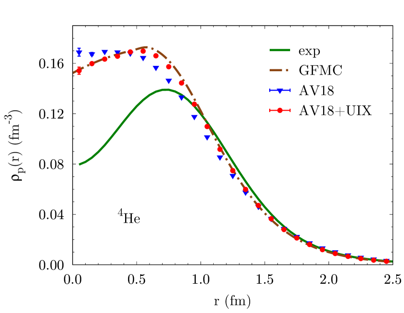
Figure 1: Point proton densities in ⁴He. The solid green line refers to the “experimental” result; see text for details. The dash-dotted brown line is the GFMC result for AV18+UIX R. B. Wiringa .

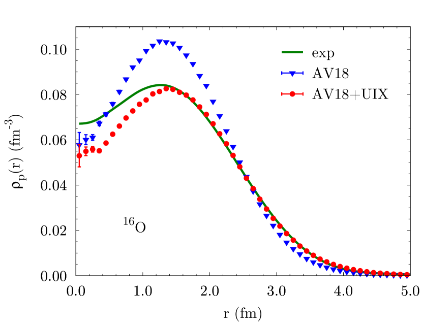
Figure 2: Point proton densities in ¹⁶O. The green line refers to the “experimental” result; see text for details.

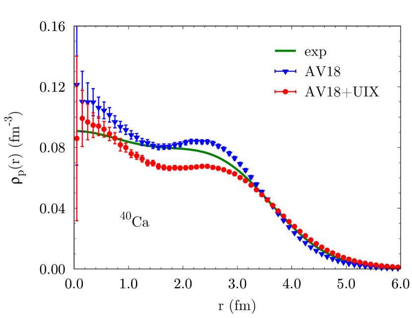
Figure 3: Point proton densities in ⁴⁰Ca. The green line refers to the “experimental” result; see text for details.

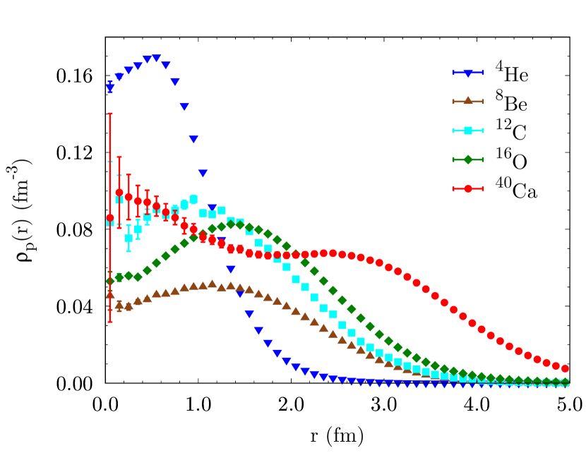
Figure 4: Point proton densities for AV18+UIX. ⁴He, ¹⁶O, and ⁴⁰Ca are the results of this work. ⁸Be and ¹²C are VMC results collected in R. B. Wiringa .

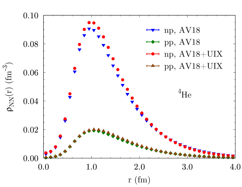
Figure 5: Two-nucleon densities of ⁴He.

Figure 6: Two-nucleon densities of ¹⁶O.

It is interesting to compare the densities of these nuclei in which $\alpha$-clustering can potentially occur. In Fig. 4 we collect the CVMC results for the point proton densities of ⁴He, ¹⁶O, and ⁴⁰Ca obtained with AV18+UIX together with those for ⁸Be and ¹²C coming from VMC calculations using the same interaction R. B. Wiringa . The ⁴He density shows a very large point density at small distance. When integrated over the volume, about half the nucleons reside inside $1.25\,\rm fm$, where the density is above $0.08\,\rm fm^{-3}$. The ⁸Be density has a low, broad peak with half the nucleons residing inside $2.25\,\rm fm$, consistent with a two-$\alpha$ cluster structure as observed in Fig. 15 of Ref. Wiringa et al. (2000). The ¹²C density peaks at a slightly smaller distance and noticeably higher value, with a larger dip at the center. This is consistent with a more tightly bound three-$\alpha$ cluster—either in a triangular configuration with a low-density region at the center of mass, or alternatively with one $\alpha$ in the $s$-shell and two $\alpha$’s in the $p$-shell. Similarly, ¹⁶O can be viewed as a tetrahedral four-$\alpha$ cluster with the $\alpha$’s at somewhat greater distance from the center of mass, or as one $s$-shell and three $p$-shell $\alpha$’s with a larger dip-peak difference than in ¹²C. The ⁴⁰Ca density is more complicated, but might be thought of as two $s$-shell $\alpha$’s giving a larger central peak, while three $p$-shell and five $d$-shell $\alpha$’s give a broad shoulder at $1-3\,\rm fm$.

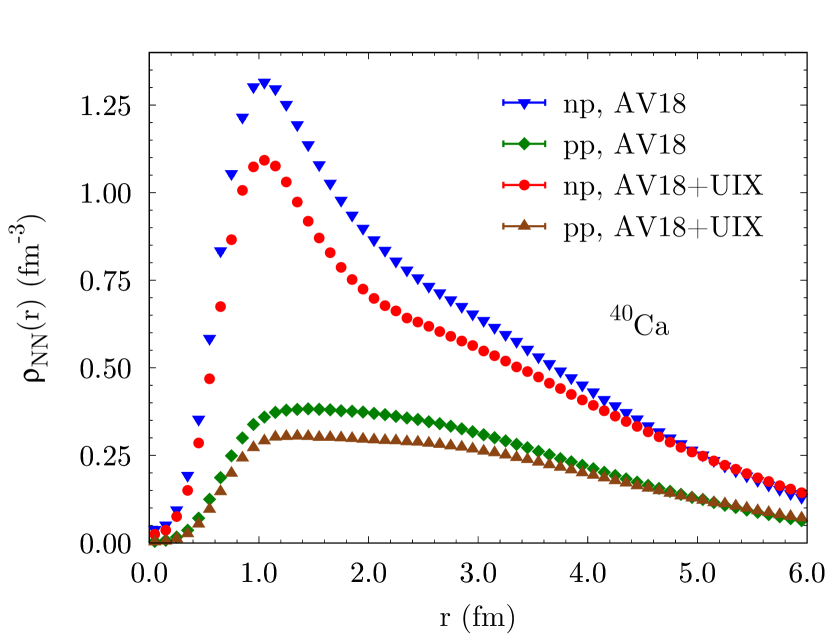
Figure 7: Two-nucleon densities of ⁴⁰Ca.

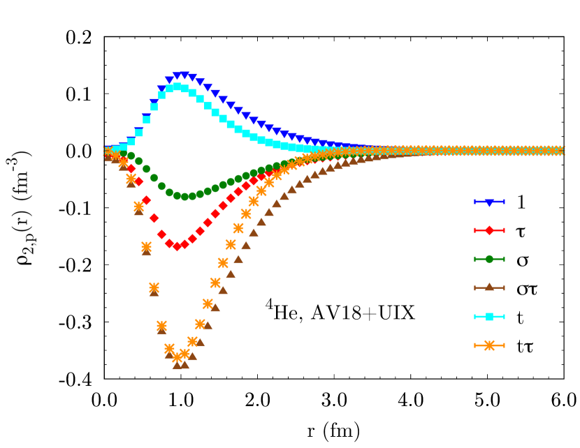
Figure 8: Operator two-nucleon densities in ⁴He. $\mathbbm{1},\,\tau,\,\sigma,\,\sigma\tau,\,t,\,t\tau$ correspond to operators $p=1,\ldots,6$ in Eq. (4).

The two-nucleon point densities of ⁴He, ¹⁶O, and ⁴⁰Ca are reported in Figs. 5, 6 and 7, respectively, for both AV18 and AV18+UIX. Upper and lower curves refer to $np$ and $pp$ pairs, respectively. The fact that $\rho_{\rm{NN}}$ is very small for $r\simeq 0$ is a consequence of the repulsive core of the $N\!N$ potential. As observed for the point-proton densities, the effect of the $3N$ force on the two-nucleon densities is appreciably different in light- and medium-heavy systems. In ⁴He the $pp$ density is almost unchanged, while the $np$ density is enhanced around the peak at $1.1\,\rm fm$. In heavier systems there is a severe depletion of both $pp$ and $np$ densities, again due to the peculiar repulsive effect of the UIX potential that tends to push nucleons apart.

Both figures and tables for the CVMC single-nucleon and two-nucleon point densities for ¹⁶O and ⁴⁰Ca, together with the VMC results for $A\leq 12$, are available online R. B. Wiringa ; R. B. Wiringa .

The two-nucleon operator point densities are shown in Figs. 8, 9 and 10 for ⁴He, ¹⁶O, and ⁴⁰Ca, respectively. It can be observed that the larger the system, the wider the range of central two-body density. In fact, the central two-body operator density is just the sum of $pp$, $np$, and $nn$ densities in Figs. 5, 6 and 7. On the other hand, spin-isospin densities are appreciably nonvanishing only for $r\lesssim 3.5\,\rm fm$, and are largely independent of the nucleus, with the position of the peaks situated around $1\,\rm{fm}$. This extends the results of Ref. Feldmeier et al. (2011), where the two-body densities normalized at short distances in $A=3$ and $A=4$ systems exhibit a universal behavior up to about $1\,\rm{fm}$ in all nuclei. Among the spin-isospin densities, $\rho_{2,\sigma\tau}$ and $\rho_{2,t\tau}$ are characterized by longer ranges and larger amplitudes, as they arise from the one-pion-exchange part of the $N\!N$ interaction. These results are qualitatively consistent with the findings of Ref. Alvioli et al. (2005), although no $3N$ forces were employed in that work. The peak values of the $\rho_{2,\sigma\tau}$ and $\rho_{2,t\tau}$ scale as $1:4:10$ for ${{}^{4}\rm He}:{{}^{16}\rm O}:{{}^{40}\rm Ca}$, or just as the number of $\alpha$-particle clusters.

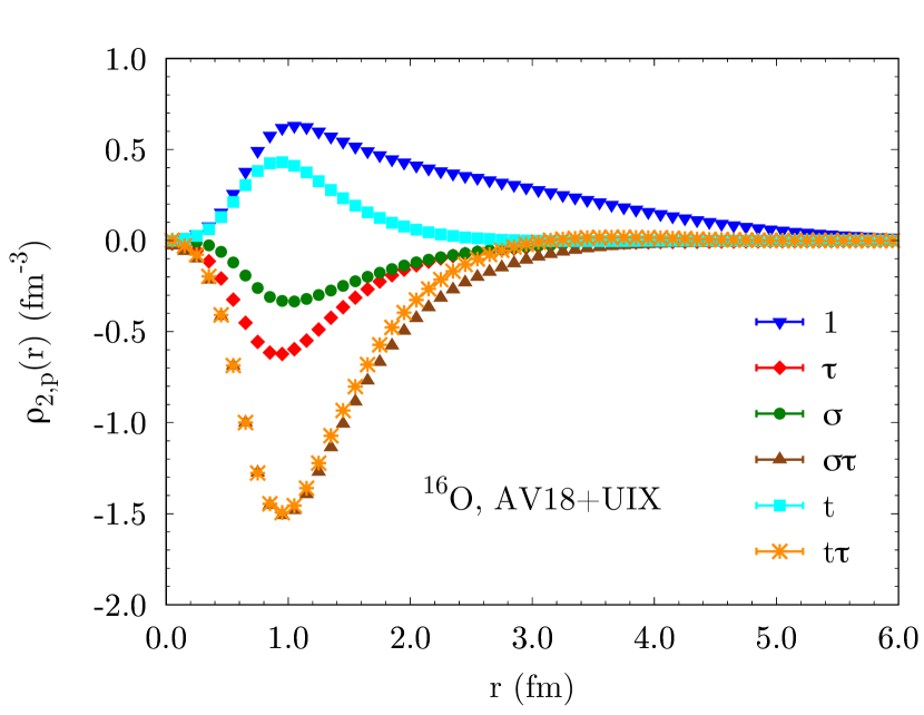
Figure 9: Operator two-nucleon densities in ¹⁶O.

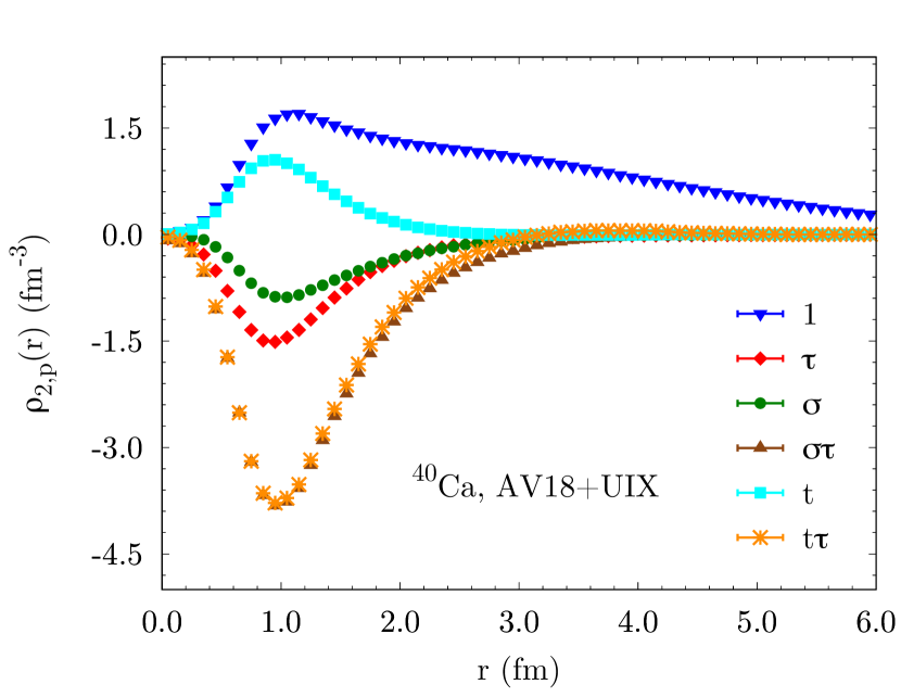
Figure 10: Operator two-nucleon densities in ⁴⁰Ca.

IV.2 Momentum distributions

The probability of finding a proton or neutron with momentum $\bm{k}$ is proportional to the momentum distribution,

$$n_{N}(\bm{k}) =\int d\bm{r}_{1}^{\prime}\,d\bm{r}_{1}^{\phantom{\prime}}\,d\bm{r}_{2}^{\phantom{\prime}}\cdots d\bm{r}_{A}^{\phantom{\prime}}\,\Psi^{\dagger}(\bm{r}_{1}^{\prime},\bm{r}_{2}^{\phantom{\prime}},\ldots,\bm{r}_{A}^{\phantom{\prime}})$$

$$\times e^{-i\bm{k}\cdot(\bm{r}_{1}^{\phantom{\prime}}-\bm{r}_{1}^{\prime})}\,\mathcal{P}_{N_{1}}\,\Psi(\bm{r}_{1}^{\phantom{\prime}},\bm{r}_{2}^{\phantom{\prime}},\ldots,\bm{r}_{A}^{\phantom{\prime}}),$$ (60)

which is normalized as

$$\mathcal{N}_{N}=\int\frac{d\bm{k}}{(2\pi)^{3}}\,n_{N}(\bm{k}),$$ (61)

$\mathcal{N}_{N}$ being the number of protons or neutrons ($\mathcal{N}_{p}\equiv Z$). In this work we present results for symmetric nuclei implying $n_{p}(\bm{k})=n_{n}(\bm{k})$. Equation (60) can be rewritten as

$$n_{N}(\bm{k}) =\frac{1}{A}\sum_{i}\int d\bm{r}_{1}\cdots d\bm{r}_{i}\cdots d\bm{r}_{A}\int d\Omega_{x}\int_{0}^{x_{\max}}dx\,x^{2}$$

$$\times\Psi^{\dagger}(\bm{r}_{1},\ldots,\bm{r}_{i},\ldots,\bm{r}_{A})\,e^{-i\bm{k}\cdot\bm{x}}$$

$$\times\mathcal{P}_{N_{i}}\,\Psi(\bm{r}_{1},\ldots,\bm{r}_{i}+\bm{x},\ldots,\bm{r}_{A})\,.$$ (62)

The Fourier transform can be computed by Monte Carlo integration. Spatial configurations are sampled as explained in Sec. III.2. The average over all particles $i$ in each configuration is then performed, and for each particle, a grid of Gauss-Legendre points $x_{i}$ is used to compute the Fourier transform. The polar angle $d\Omega_{x}$ is also sampled by Monte Carlo integration, with a randomly chosen direction for each particle in each configuration. For all the nuclei under study we calculated $n(\bm{k})$ up to $k=10\,\rm fm^{-1}$, integrating to $x_{\max}=20\,\rm fm$ using 200 Gauss-Legendre points.

As reported in Ref. Pieper et al. (1992), with the employed expansion the three-body clusters give small contribution to the momentum distribution. In this work, $n_{N}(\bm{k})$ is evaluated up to three-body cluster and then extrapolated using Eq. 55. In order to save computing time, spin-orbit correlations are turned off in the calculation of the momentum distribution. This approximation, also used in standard VMC calculations Wiringa et al. (2014), is justified by the small effect of spin-orbit correlations on $n_{N}(\bm{k})$ compared to the first six operators of the two-body correlations. The results for ⁴He, ¹⁶O, and ⁴⁰Ca are shown in Figs. 11, 12 and 13, respectively. For $A=4$ the VMC result for AV18+UIX Wiringa is also displayed for comparison. The proton momentum distributions are reported for both AV18 and AV18+UIX. The $3N$ force makes only small changes to $n_{N}(\bm{k})$. Near $k=2\,\rm fm^{-1}$ the momentum distribution manifests a sharp change in slope, as previously observed in both light- Wiringa et al. (2014) and medium-mass Alvioli et al. (2008) nuclei. This is attributed to the strong tensor correlations induced by the one-pion-exchange part of the $N\!N$ potential, further enhanced by the two-pion-exchange part of the $3N$ potential, when included. At higher momentum, the tail of $n_{N}(\bm{k})$ manifests the expected universal behavior determined by the short-range correlations, i.e., by the short-range structure of the employed Hamiltonian, as shown in Fig. 14 and discussed at length in a number of other works Feldmeier et al. (2011); Alvioli et al. (2012, 2013, 2016). Such universality refers to the independence of the tail with respect to the specific nucleus. On the other hand, the high-momentum tail strongly depends on the nuclear interaction model. The recently developed local chiral interactions, which are significantly softer than the phenomenological interactions employed in this work, yield a momentum distribution characterized by weaker high-momentum components Gandolfi et al. than those of Figs. 11, 12 and 13.

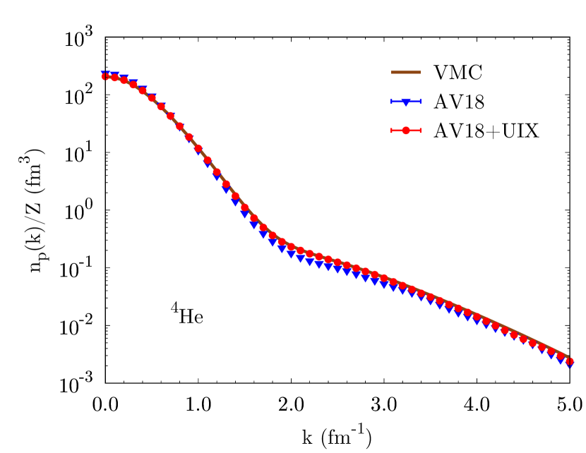
Figure 11: Proton momentum distributions in ⁴He. Averages are calculated on $\mathcal{N}_{c}=10^{7}$ configurations. The brown line is the VMC result for AV18+UIX Wiringa .

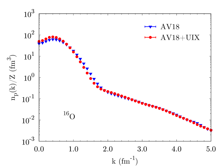
Figure 12: Proton momentum distributions in ¹⁶O. Averages are calculated on $\mathcal{N}_{c}=10^{7}$ configurations for AV18, and on $\mathcal{N}_{c}=8\times 10^{6}$ configurations for AV18+UIX.

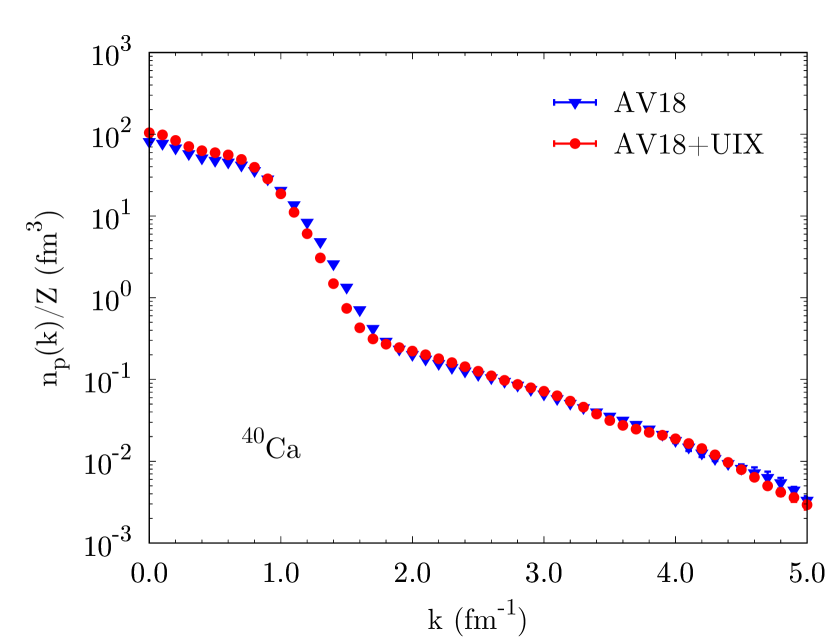
Figure 13: Proton momentum distributions in ⁴⁰Ca. Averages are calculated on $\mathcal{N}_{c}=10^{7}$ configurations for AV18, and on $\mathcal{N}_{c}=8\times 10^{6}$ configurations for AV18+UIX.

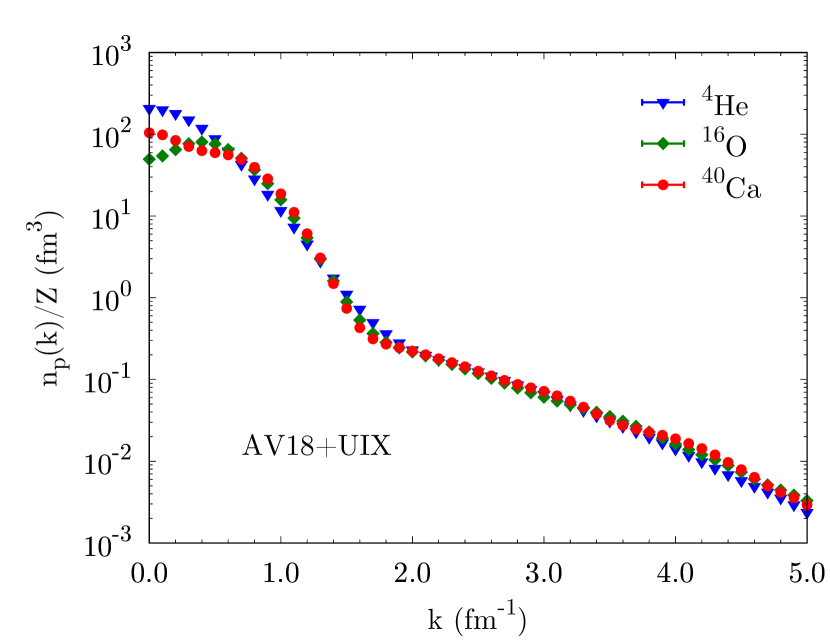
Figure 14: Proton momentum distributions for AV18+UIX.

Compared to the other local or nearly local operators, like the kinetic energy, the potential energy, and the densities, the momentum distribution is strictly a nonlocal operator. In order to check the convergence of the cluster expansion for such operator we computed the kinetic energy by integrating the momentum distribution

$$E_{N}^{\rm kin}(k)=\frac{\hbar^{2}}{2m_{N}}4\pi\int_{0}^{k}dk^{\prime}\,k^{\prime\,4}\,n_{N}(k^{\prime}),$$ (63)

for each order of the expansion. The contributions for ¹⁶O with AV18+UIX up to $k=10\,\rm fm^{-1}$ are $16.3(2)\,\rm MeV/A$ for one-body cluster, $16.0(5)\,\rm MeV/A$ for two-body cluster, and $-4.4(4)\,\rm MeV/A$ for three-body cluster. The integration of the extrapolated $n_{N}(\bm{k})$ leads to $28.9(6)\,\rm MeV/A$. This is compatible with the cluster contributions reported in the first line of Table 4. The missing 4- to 16-body cluster contributions to the integrated kinetic energy, that account for $\simeq 1\,\rm MeV/A$, are fully recovered by the extrapolation of $n_{N}(\bm{k})$. This validates the convergence of the expansion and confirms the negligible effect of spin-orbit correlations on the momentum distribution. Similar outcomes are found for the other nuclei considered in this work. The errors on the integrated kinetic energies are larger than those of the direct calculation because of the propagation of uncertainties in the integration of $n_{N}(\bm{k})$, which above $5\,\rm fm^{-1}$ has large statistical errors due to the cancellation of positive and negative small cluster contributions. However, as discussed in the next paragraph, the integrated strength of the momentum distribution saturates before $5\,\rm fm^{-1}$. Simulations for $n_{N}(\bm{k})$ have been thus carried out with good statistics up to that momentum value, using up to $10^{7}$ Monte Carlo configurations.

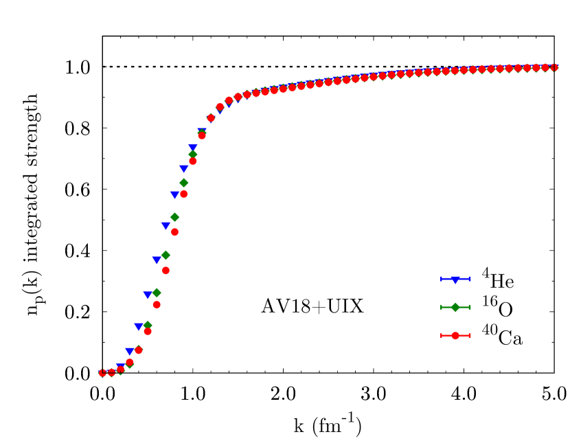
Figure 15: Integrated strengths for AV18+UIX. See text for details.

The momentum distribution integrated strength as a function of $k$ is reported in Fig. 15 for AV18+UIX. At low momentum it decreases as $A$ increases, because the nuclei become more tightly bound, and the fraction of nucleons at low momentum decreases. At $k=2\,\rm fm^{-1}$ for all the systems analyzed, the integrated strength is already $\simeq 93\%$ of the total, and it becomes $\simeq 99\%$ at $k=4\,\rm fm^{-1}$. Less than $1\%$ of the total strength is given by the tail of the momentum distribution above $4\,\rm fm^{-1}$.

The figures and the tables for the CVMC momentum distributions for ¹⁶O and ⁴⁰Ca, together with the VMC results for $A\leq 12$, are available online Wiringa .

IV.3 Charge form factors and Coulomb sum rules

The double differential cross section of the inclusive electron-nucleus scattering process in which an electron of initial four-momentum $k_{e}=(\bm{k}_{e},E_{e})$ scatters off a nuclear target to a state of four-momentum $k_{e}^{\prime}=(\bm{k}_{e}^{\prime},E_{e}^{\prime})$, the hadronic final state being undetected, can be written in the one-photon-exchange approximation as

$$\!\!\!\frac{d^{2}\sigma}{dE_{e^{\prime}}d\Omega_{e^{\prime}}}\!=\!\left(\frac{d\sigma}{d\Omega_{e^{\prime}}}\right)_{\!\rm M}\!\Big{[}A_{L}R_{L}({\bm{q}},\omega)+A_{T}R_{T}({\bm{q}},\omega)\Big{]},$$ (64)

where

$$A_{L}=\left(\frac{Q^{2}}{\bm{q}^{2}}\right)^{2},\qquad A_{T}=\frac{1}{2}\frac{Q^{2}}{\bm{q}^{2}}+\tan^{2}\frac{\theta_{e^{\prime}}}{2},$$ (65)

and

$$\left(\frac{d\sigma}{d\Omega_{e^{\prime}}}\right)_{\!\rm M}=\left[\frac{\alpha\cos{\displaystyle\frac{\theta_{e^{\prime}}}{2}}}{2E_{e}\sin^{2}{\displaystyle\frac{\theta_{e^{\prime}}}{2}}}\right]^{2}$$ (66)

is the Mott cross section. In the above expressions, $\alpha\simeq 1/137$ is the fine structure constant, $d\Omega_{e^{\prime}}$ is the differential solid angle in the direction of $\bm{k}_{e^{\prime}}$, $q=k_{e}-k_{e^{\prime}}=(\bm{q},\omega)$ is the four-momentum transfer, and $Q^{2}=-q^{2}=\bm{q}^{2}-\omega^{2}$. The longitudinal and transverse response functions are defined as

$$R_{\alpha}(\bm{q},\omega) =\sum_{f}\langle f|j_{\alpha}({\bm{q}},\omega)|0\rangle\langle f|j_{\alpha}({\bm{q}},\omega)|0\rangle^{*}$$

$$\times\delta(E_{f}-\omega-E_{0}),\qquad\alpha=L,T,$$ (67)

where $|0\rangle$ and $|f\rangle$ represent the nuclear initial and final states of energies $E_{0}$ and $E_{f}$, and $j_{L}({\bm{q}},\omega)$ and $j_{T}({\bm{q}},\omega)$ are the electromagnetic charge and current operators, respectively.

Recently, the quasielastic electromagnetic response functions of ⁴He and ¹²C have been computed within GFMC using realistic nuclear two- and three-body forces and consistent one- and two-body electroweak currents Lovato et al. (2015, 2016). Besides the transverse enhancement brought about by two-body current contributions, the authors of Ref. Lovato et al. (2016) have found no evidence of in-medium modification of the nucleon form factor in the analysis of the longitudinal response function of ¹²C. This is at variance with the findings of Ref. Cloët et al. (2016), where changes to the proton Dirac form factor induced by the nuclear medium leads to a dramatic quenching of the Coulomb sum rule,

$$S_{L}(\bm{q})=\frac{1}{Z}\int_{w_{\rm th}^{+}}^{\infty}d\omega\,\frac{R_{L}(\bm{q},\omega)}{G_{E}^{p\,2}(Q^{2})},$$ (68)

where $\omega_{\rm th}$ is the energy transfer corresponding to the inelastic threshold, and $G_{E}^{p}(Q^{2})$ is the proton electric form factor evaluated at four-momentum transfer $Q^{2}$.

The one-body charge operator employed in the GFMC calculations has the standard expressions obtained from a relativistic reduction of the time component of the covariant single-nucleon current,

$$j_{L}({\bm{q}},\omega)= \Bigg{[}\frac{\epsilon_{i}(Q^{2})}{\sqrt{1+Q^{2}/(4m^{2})}}$$

$$-i\,\frac{2\mu_{i}(Q^{2})-\epsilon_{i}(Q^{2})}{4m^{2}}\,\bm{q}\cdot({\bm{\sigma}}_{i}\times{\bm{p}}_{i})\Bigg{]}e^{i\bm{q}\cdot\bm{r}_{i}},$$ (69)

with

$$\begin{aligned} \epsilon_{i}(Q^{2})&=G^{p}_{E}(Q^{2})\frac{1+\tau_{z_{i}}}{2}+G_{E}^{n}(Q^{2})\frac{1-\tau_{z_{i}}}{2},\\ \mu_{i}(Q^{2})&=G_{M}^{p}(Q^{2})\frac{1+\tau_{z_{i}}}{2}+G_{M}^{n}(Q^{2})\frac{1-\tau_{z_{i}}}{2}\,.\end{aligned}$$ (70)

In this work we adopted Kelly’s parametrization Kelly (2004) for the nucleon electric and magnetic form factors $G^{p,n}_{E,M}$.

In $R_{L}(\bm{q},\omega)$, the $\omega$ dependence enters via the energy-conserving $\delta$ function and the four-momentum transfer $Q^{2}$ of the electroweak form factors of the nucleon. The latter can be removed by evaluating these form factors at $Q^{2}_{\rm qe}=\bm{q}^{2}-\omega^{2}_{\rm qe}$, where $\omega_{\rm qe}$ is the energy transfer corresponding to the quasielastic peak, and by dividing the response by the factor $G_{E}^{p\,2}(Q_{\rm qe}^{2})$. Therefore, the Coulomb sum rule can be very well approximated by the following ground-state expectation value

$$S_{L}(\bm{q})= \frac{1}{Z}\Big{[}\langle 0|\mathcal{O}_{L}^{\dagger}({\bm{q}})\,\mathcal{O}_{L}({\bm{q}})|0\rangle$$

$$-|\langle 0;{\bm{q}}|\mathcal{O}_{L}({\bm{q}})|0\rangle|^{2}\Big{]},$$ (71)

where $\mathcal{O}_{L}({\bm{q}})=j_{L}({\bm{q}},\omega_{\rm qe})/G_{E}^{p}(Q_{\rm qe}^{2})$ Lovato et al. (2013). The Coulomb sum rule defined in Eq. 68 only includes the inelastic contribution to $R_{\alpha}(\bm{q},\omega)$, i.e., the elastic contribution represented by the second term on the right-hand side of Eq. 71, where $|0;{\bm{q}}\rangle$ denotes the ground state of the nucleus recoiling with total momentum ${\bm{q}}$, has been removed. This term is proportional to the longitudinal elastic form factor, which is given by

$$F_{L}(\bm{q})=\frac{1}{Z}G_{E}^{p}(Q^{2}_{\rm el})\langle 0;{\bm{q}}|\mathcal{O}_{L}({\bm{q}})|0\rangle,$$ (72)

where $Q^{2}_{\rm el}=\bm{q}^{2}-\omega_{\rm el}^{2}$, and $\omega_{\rm el}$ is the energy transfer corresponding to elastic scattering, $\omega_{\rm el}=\sqrt{q^{2}+m_{A}^{2}}-m_{A}$ ($m_{A}$ is the mass of the target nucleus).

Neglecting the small spin-orbit contribution of Eq. 69, the Coulomb sum rule and the elastic form factor can be expressed as

$$S_{L}(\bm{q}) =\frac{1}{Z}\frac{1}{G_{E}^{p\,2}(Q_{\rm qe}^{2})}\frac{1}{1+Q_{\rm qe}^{2}/(4m^{2})}$$

$$\Big{\{}G_{E}^{p\,2}(Q_{\rm qe}^{2})\,\left[\tilde{\rho}_{pp}(q)+Z\right]$$

$$+G_{E}^{n\,2}(Q_{\rm qe}^{2})\,\left[\tilde{\rho}_{nn}(q)+(A-Z)\right]$$

$$+2\,G_{E}^{p}(Q_{\rm qe}^{2})\,G_{E}^{n}(Q_{\rm qe}^{2})\,\tilde{\rho}_{np}(q)$$

$$-\left[G_{E}^{p}(Q_{\rm qe}^{2})\,\tilde{\rho}_{p}(q)+G_{E}^{n}(Q_{\rm qe}^{2})\,\tilde{\rho}_{n}(q)\right]^{2}\Big{\}},$$ (73)

$$F_{L}(\bm{q}) =\frac{1}{Z}\frac{G_{E}^{p}(Q_{\rm el}^{2})\,\tilde{\rho}_{p}(q)+G_{E}^{n}(Q_{\rm el}^{2})\,\tilde{\rho}_{n}(q)}{\sqrt{1+Q_{\rm el}^{2}/(4m^{2})}}\,,$$ (74)

where $\tilde{\rho}_{N}(q)$ and $\tilde{\rho}_{\rm{NN}}(q)$ are the Fourier transform of the densities defined in Eqs. 57 and 58).

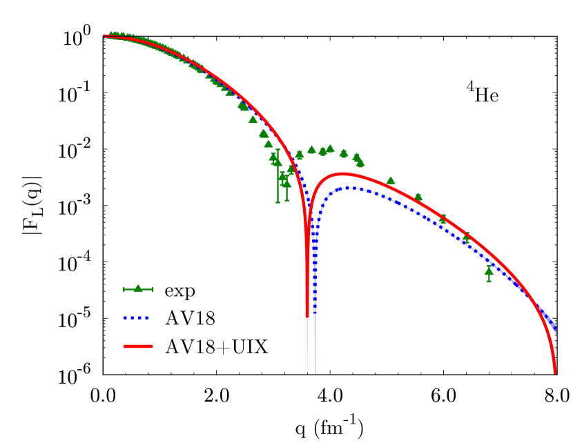
Figure 16: Longitudinal elastic form factors for ⁴He. Shaded areas indicate propagated Monte Carlo statistical errors in the Fourier transforms. Experimental data are from an unpublished compilation by I. Sick, based on Refs. Frosch et al. (1967); Erich et al. (1968); McCarthy et al. (1977); Arnold et al. (1978); Ottermann et al. (1985).

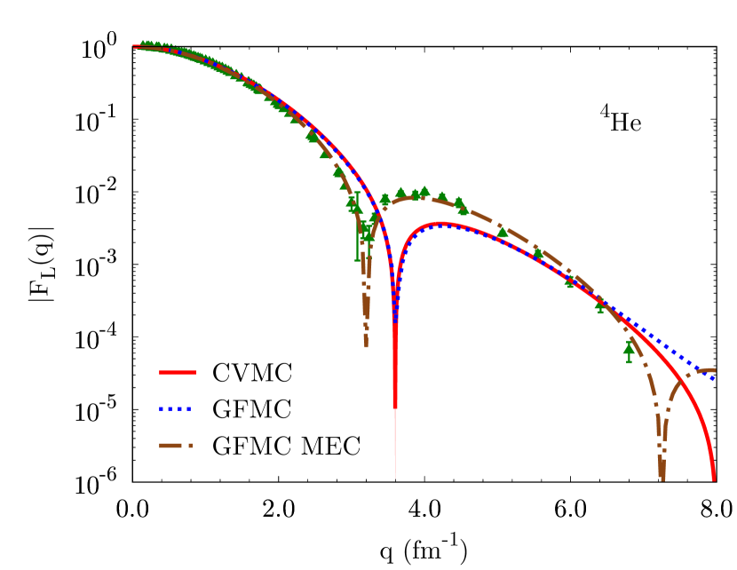
Figure 17: Longitudinal elastic form factors for ⁴He. Results employing the AV18+UIX potential are reported for CVMC and GFMC, the latter with and without MECs. Experimental results are the same as in Fig. 16.

Here we compute the Coulomb sum rules and the elastic form factors of ⁴He, ¹⁶O, and ⁴⁰Ca, to provide a useful benchmark for current and future analysis of electron-nucleus scattering data. In particular, our results for ¹⁶O and ⁴⁰Ca, when compared to experiment, should further elucidate the role of in-medium modification of the nucleon form factors.

The ⁴He longitudinal elastic form factor is compared to experimental data in Fig. 16. Our theoretical results for the AV18 interaction significantly overpredict the diffraction minimum and maximum positions. Inclusion of the $3N$ force brings theory closer to experiment, but it is known that MECs are needed to further shift the peaks of the longitudinal elastic form factor to lower values of the momentum transfer and achieve agreement with experiment Marcucci et al. (2016); Carlson et al. (2015). This is shown in Fig. 17 where the GFMC longitudinal elastic form factor with and without MEC contributions is displayed. Note that up to $\simeq 6\,\rm fm^{-1}$ the CVMC form factor perfectly matches the GFMC result obtained without MECs.

The longitudinal form factor of ¹⁶O is shown in Fig. 18. The experimental data are well reproduced by our calculations once the $3N$ force is included. In analogy to ¹²C Lovato et al. (2013), it is plausible that two-body current contributions are negligible at low $q$, and become appreciable only for $q>3\,\rm fm^{-1}$. In fact, in the high-momentum region MECs interfere destructively with the one-body contributions, bringing theoretical prediction of ¹²C into closer agreement with experiment. This is consistent with the findings of Ref. Mihaila and Heisenberg (2000), where MECs improve the description of ¹⁶O experimental data above $2.5\,\rm fm^{-1}$.

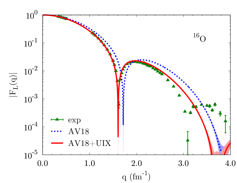
Figure 18: Longitudinal elastic form factors for ¹⁶O. Shaded areas indicate propagated Monte Carlo statistical errors in the Fourier transforms. Experimental data are from an unpublished compilation by I. Sick, based on Refs. Sick and McCarthy (1970); Schuetz (1975); Sick .

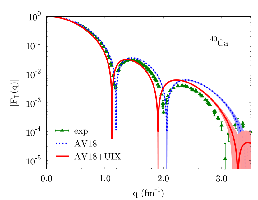
Figure 19: Longitudinal elastic form factors for ⁴⁰Ca. Shaded areas indicate propagated Monte Carlo statistical errors in the Fourier transforms. Experimental data are from an unpublished compilation by I. Sick, based on Refs. Sinha et al. (1973); Sick ; Sick et al. (1979).

As for the ⁴⁰Ca nucleus, a better agreement with experiments is achieved when AV18 only is present in the Hamiltonian (see Fig. 19). Assuming that, as for ¹²C and ¹⁶O, two-body current contributions have little effect for $q\leq 3\,\rm fm^{-1}$, we can infer that the UIX potential moves the diffraction peaks to excessively low values of $q$. This failure of the UIX interaction is directly related to the behavior of the point proton density displayed in Fig. 3, where nucleons are pushed too far away from the center of mass when UIX is employed.

The longitudinal sum rules of ⁴He, ¹⁶O, and ⁴⁰Ca for AV18+UIX obtained from Section IV.3 are displayed in Fig. 20. The best GFMC estimates for $S_{L}(\bm{q})$ in ⁴He and ¹²C Lovato et al. (2013) are also shown for comparison (solid symbols). GFMC calculations have been carried out employing the AV18+IL7 potential and considering the full contribution of one- and two-body electromagnetic currents. The latter have only a relatively small effect on the longitudinal sum rule, mainly affecting the magnitude of the peak for ¹²C and the region above $3\,\rm fm^{-1}$. In this region, in addition to MECs, the discrepancies between CVMC and GFMC are due to the spin-orbit contribution in the charge operator, neglected in CVMC calculations but included in Ref. Lovato et al. (2013). In the large $q$ limit, the CVMC sum rules differ from unity because of relativistic corrections in the charge current, which gives the factor $1/(1+Q_{\rm qe}^{2}/(4m^{2}))$ of Section IV.3.

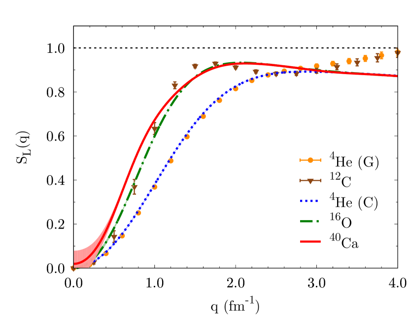
Figure 20: Coulomb sum rules for $A\leq 40$. Symbols with statistical error bars show GFMC calculations employing the AV18+IL7 potential Lovato et al. (2013). The curves show CVMC results for AV18+UIX. Shaded areas indicate propagated Monte Carlo statistical errors in the Fourier transforms.

Extracting the Coulomb sum rules from the experimental response functions involves nontrivial difficulties. The experimental determination of $S_{L}(\bm{q})$ requires measuring the associated $R_{L}(\bm{q},\omega)$ from the inelastic threshold to infinity. However, inclusive electron scattering experiments can only explore the space-like region of the four-momentum transfer $\omega<q$. Therefore, a meaningful comparison between theory and experiment requires estimating the strength outside the region covered by electron-scattering experiments. Furthermore, the authors of Ref. Lovato et al. (2016) have shown that the transitions to the low-lying states of ¹²C give significant contributions to $\langle 0|\mathcal{O}^{\dagger}_{L}(\bm{q})\mathcal{O}_{L}(\bm{q})|0\rangle$ that are not present in the longitudinal response functions extracted from inclusive $(e,e^{\prime})$ cross sections. Therefore, before comparing experiment with the present theory, which computes the sum rule of the total inelastic response rather than just the quasielastic one, these contributions have to be explicitly removed from the theoretical sum rule. In the ¹²C case, the transition form factors to $J^{\pi}=2^{+}$, $0_{2}^{+}$ (Hoyle), and $4^{+}$ states were taken from experiments. However, this approach is not suitable to the present work because of the large numbers of low-lying transitions of ¹⁶O and ⁴⁰Ca. For this reason we refrain from reporting experimental data in Fig. 20.

V Conclusions

A variational Monte Carlo analysis of the properties of three closed-shell nuclei, ⁴He, ¹⁶O, and ⁴⁰Ca, has been performed. We employed the accurate phenomenological nuclear Hamiltonian AV18+UIX, which is capable of simultaneously describing two-nucleon bound and scattering states, the binding energy of ⁴He, and the saturation density of isospin-symmetric nuclear matter. The CVMC algorithm has been improved by including five-body terms in the cluster expansion of all the spin-isospin dependent correlations. Therefore, this work represents significant progress with respect to Ref. Pieper et al. (1990, 1992), in which the older AV14+UVII Hamiltonian was employed, the cluster expansion was limited to four-body terms only, spin-orbit correlations were treated only at two-body cluster level, and other approximations were made in the construction of the wave function and in estimating the variational expectation values.

In order to perform extensive searches for the optimal variational parameters in the multidimensional parameter space defined by the employed wave functions, we implemented in the CVMC program the open-source library for nonlinear optimization NLopt Johnson . The accuracy of the optimized wave function has been tested against standard VMC and GFMC calculations for ⁴He using both AV18 and AV18+UIX, and against AFDMC results for ⁴He and ¹⁶O employing the AV6^′ potential.

We present results for the binding energy, charge radius, one- and two-body densities, single-nucleon momentum distribution, charge form factor, and Coulomb sum rule, fully accounting for the high-momentum components of the nuclear interaction. We find that the UIX three-body potential, known to be attractive for $A\leq 12$, becomes repulsive for $A\geq 16$. At variance with the ⁴He case, the addition of the UIX potential makes ¹⁶O and ⁴⁰Ca less bound. This repulsive effect is not limited to the binding energies. In ¹⁶O and ⁴⁰Ca nucleons are pushed far away from the center of mass when the $3N$ force is included, resulting in larger radii, broader densities, and a shift of the charge form factor diffraction peaks towards smaller momenta. Although relying on different interaction schemes, a similar behavior of three-body interactions is found in CC and IM-SRG calculations for medium-heavy nuclei (see Hagen et al. (2014); Hebeler et al. (2015); Hergert et al. (2016) and references therein). We note that within CVMC there is no need to soften the $N\!N$ potential and to employ either the normal ordering procedure or a two-body density dependent approximation for the three-body force.

Although the UIX three-nucleon interaction manifests a change in behavior—from attractive to repulsive—for $A\geq 16$, it appears to provide a better description of radii, densities and charge form factors, of nuclei at least up to $A=16$. For instance, the charge radius and the position of the first peak in the longitudinal elastic form factor of ¹⁶O are better reproduced by the full AV18+UIX interaction than by the AV18 potential alone. This is no longer true in ⁴⁰Ca, where the inclusion of the $3N$ potential yields a too large charge radius and shifts the diffraction peaks of the charge form factor towards too small momenta. The experimental data for ⁴⁰Ca lie in between the CVMC theoretical predictions for AV18 and AV18+UIX. The fact that the AV18+UIX Hamiltonian is not adequate to describe medium-mass nuclei is consistent with the deficiencies in the theoretical prediction of isospin-symmetric nuclear matter employing the same interaction. Although the correct saturation density is obtained, the binding energy per nucleon is too small Akmal et al. (1998). In this regard, as a follow up of this work, we will consider local $N\!N$ potentials recently derived in coordinate space within chiral perturbation theory Gezerlis et al. (2013, 2014); Piarulli et al. (2015, 2016); Tews et al. (2016); Lynn et al. (2016); Logoteta et al. (2016). The latter are characterized by a spin-isospin structure analogous to the one of AV18+UIX so the CVMC can be straightforwardly extended to this class of interactions. It will be interesting to see whether local chiral effective field theory Hamiltonians provide a satisfactory description of ¹⁶O, ⁴⁰Ca, and light nuclei.

Figure 21: Central correlation functions for AV18 and AV18+UIX for $A=4$ and $A>4$ (the same two-body correlations have been employed in ¹⁶O and ⁴⁰Ca; see text for details).

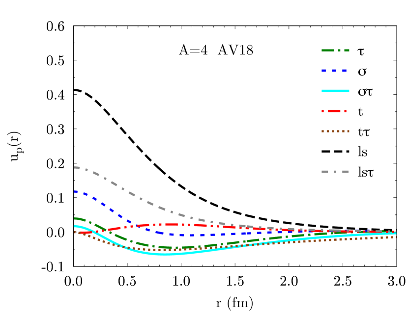
Figure 22: Radial correlation functions for $A=4$ and AV18. $\tau,\,\sigma,\,\sigma\tau,\,t,\,t\tau,\,ls,\,ls\tau$ correspond to operators $p=2,\ldots,8$ in Eqs. (4) and (6).

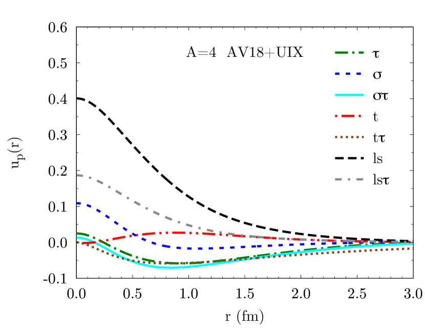
Figure 23: Radial correlation functions for $A=4$ and AV18+UIX.

We also computed the single-nucleon momentum distributions of ¹⁶O and ⁴⁰Ca. These extend the VMC collection of Refs. Wiringa et al. (2014); Wiringa obtained using realistic phenomenological Hamiltonians, which include both $N\!N$ and $3N$ interactions. Together with the inclusion of three-body and higher-order terms in the cluster expansion, this makes the calculations of $n(\bm{k})$ accurate in both the high- and low-momentum regions. The universality of the tail of the momentum distribution, i.e., the independence of the high-momentum component upon the specific nucleus, has been confirmed for the selected interaction scheme. The momentum distributions are of immediate use for the studies of the high-momentum structure of nuclei, which includes the EMC effect and the analysis of short-range correlations in nuclei Arrington (2016). For the latter, the analysis of two-nucleon momentum distributions derived employing realistic two- and three-body nuclear interactions will be of great interest. A future project will focus on the CVMC computation of two-nucleon momentum distributions in medium-heavy nuclei, extending the VMC collection of Refs. Wiringa et al. (2014); R. B. Wiringa and providing a comparison with the findings of Ref. Alvioli et al. (2016).

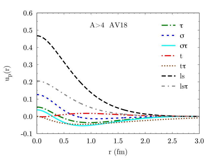
Figure 24: Radial correlation functions for $A>4$ and AV18.

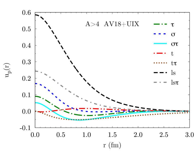
Figure 25: Radial correlation functions for $A>4$ and AV18+UIX.

We plan to employ the momentum distributions, and the average separation energies, computed in this work to evaluate the electroweak response functions of ¹⁶O and ⁴⁰Ca in the impulse approximation, with particular emphasis on the role of three-nucleon forces, extending the study of Ref. Bacca et al. (2009) to heavier nuclei. This will be relevant for neutrino-oscillation experiments, such as the Deep Underground Neutrino Experiment (DUNE) Deep Underground Neutrino Experiment , and to elucidate quark and gluon effects in nuclei, which have long been actively sought, but never unambiguously identified.

Table 11: Variational parameters for ⁴He, ¹⁶O, and ⁴⁰Ca.

param	4He		16O		40Ca
	AV18	AV18+UIX	AV18	AV18+UIX	AV18	AV18+UIX
$V_{S}$	$-47.824\,\rm MeV$	$-51.459\,\rm MeV$	$-44.860\,\rm MeV$	$-43.032\,\rm MeV$	$-47.261\,\rm MeV$	$-45.606\,\rm MeV$
$R_{s}$	$2.174\,\rm fm$	$2.039\,\rm fm$	$3.325\,\rm fm$	$3.542\,\rm fm$	$4.592\,\rm fm$	$4.872\,\rm fm$
$a_{s}$	$0.371\,\rm fm$	$0.340\,\rm fm$	$0.439\,\rm fm$	$0.641\,\rm fm$	$0.690\,\rm fm$	$0.930\,\rm fm$
$\alpha_{s}$	$0.126$	$0.285$	$-0.056$	$-0.091$	$-0.056$	$-0.091$
$\rho_{s}$	$1.643\,\rm fm$	$1.131\,\rm fm$	$1.847\,\rm fm$	$1.009\,\rm fm$	$1.847\,\rm fm$	$1.009\,\rm fm$
$k_{F}$	$1.864\,\rm fm^{-1}$	$1.7036\,\rm fm^{-1}$	$1.604\,\rm fm^{-1}$	$1.309\,\rm fm^{-1}$	$1.604\,\rm fm^{-1}$	$1.309\,\rm fm^{-1}$
$\alpha$	$0.759$	$0.745$	$0.787$	$0.893$	$0.787$	$0.893$
$\beta_{c}$	$0.976$	$0.994$	$1.078$	$1.172$	$1.078$	$1.172$
$\beta_{t}$	$1.206$	$1.341$	$1.130$	$1.194$	$1.130$	$1.194$
$d_{\rm S}$	$3.361\,\rm fm$	$3.539\,\rm fm$	$2.787\,\rm fm$	$2.502\,\rm fm$	$2.787\,\rm fm$	$2.502\,\rm fm$
$d_{\rm P}$	$4.711\,\rm fm$	$4.039\,\rm fm$	$2.867\,\rm fm$	$3.212\,\rm fm$	$2.867\,\rm fm$	$3.212\,\rm fm$
$d_{t}$	$6.449\,\rm fm$	$6.716\,\rm fm$	$4.655\,\rm fm$	$4.312\,\rm fm$	$4.655\,\rm fm$	$4.312\,\rm fm$
$t_{1}$	$5.792$	$5.769$	$5.165$	$4.097$	$5.165$	$4.097$
$t_{2}$	$4$	$4$	$4$	$4$	$4$	$4$
$t_{3}$	$0.127\,\rm fm^{-1}$	$0.117\,\rm fm^{-1}$	$0.252\,\rm fm^{-1}$	$0.202\,\rm fm^{-1}$	$0.252\,\rm fm^{-1}$	$0.202\,\rm fm^{-1}$
$\varepsilon_{2\pi,A}$		$-9.60\cdot 10^{-4}$		$-8.77\cdot 10^{-4}$		$-8.77\cdot 10^{-4}$
$\varepsilon_{R}$		$-8.22\cdot 10^{-4}$		$-7.87\cdot 10^{-4}$		$-7.87\cdot 10^{-4}$
$\eta$		$0.693$		$1.005$		$1.005$
$c_{y}$		$1.337\,\rm fm^{-2}$		$1.601\,\rm fm^{-2}$		$1.619\,\rm fm^{-2}$
$c_{t}$		$1.811\,\rm fm^{-2}$		$1.616\,\rm fm^{-2}$		$1.734\,\rm fm^{-2}$

We computed the Coulomb sum rules for closed-shell nuclei ranging from $A=4$ to $A=40$. Our calculations show very little $A$ dependence of the sum rules for $A\geq 12$ for momentum transfers as low as $1\,\rm fm^{-1}$. These results are also consistent with the recent GFMC calculation for ¹²C Lovato et al. (2016).

Another future project will be to examine closed-shell nuclei $+/-$ one nucleon, e.g., ¹⁵N, ¹⁵O, ¹⁷O, ¹⁷F, to study various properties such as spin-orbit splitting, which was previously evaluated in ¹⁵N using CVMC in Ref. Pieper and Pandharipande (1993), charge-symmetry breaking Wiringa et al. (2013), and $\beta$ decay.

Appendix: Wave function details

Figures 21, 22, 23, 24 and 25 and Table 11 provide the radial correlation functions and all the variational parameters for the systems under study for both AV18 and AV18+UIX.

References

- Carlson et al. (2015) J. Carlson, S. Gandolfi, F. Pederiva, S. C. Pieper, R. Schiavilla, K. E. Schmidt, and R. B. Wiringa, Rev. Mod. Phys. 87, 1067 (2015).
- Akmal et al. (1998) A. Akmal, V. R. Pandharipande, and D. G. Ravenhall, Phys. Rev. C 58, 1804 (1998).
- Carbone et al. (2014) A. Carbone, A. Rios, and A. Polls, Phys. Rev. C 90, 054322 (2014).
- Logoteta et al. (2016) D. Logoteta, I. Bombaci, and A. Kievsky, Phys. Rev. C 94, 064001 (2016).
- Wiringa et al. (1995) R. B. Wiringa, V. G. J. Stoks, and R. Schiavilla, Phys. Rev. C 51, 38 (1995).
- Pieper et al. (2001) S. C. Pieper, V. R. Pandharipande, R. B. Wiringa, and J. Carlson, Phys. Rev. C 64, 014001 (2001).
- Pieper (2008a) S. C. Pieper, AIP Conference Proceedings 1011, 143 (2008a).
- Pieper (2008b) S. C. Pieper, Riv. Nuovo Cim. 31, 709 (2008b).
- Maris et al. (2013) P. Maris, J. P. Vary, S. Gandolfi, J. Carlson, and S. C. Pieper, Phys. Rev. C 87, 054318 (2013).
- Gandolfi et al. (2012) S. Gandolfi, J. Carlson, and S. Reddy, Phys. Rev. C 85, 032801 (2012).
- Steiner and Gandolfi (2012) A. W. Steiner and S. Gandolfi, Phys. Rev. Lett. 108, 081102 (2012).
- (12) Facility for Rare Isotope Beams, http://www.frib.msu.edu/.
- Ankowski et al. (2016) A. Ankowski, J. Beacom, O. Benhar, S. Chen, J. Cherry, Y. Cui, A. Friedland, I. Gil-Botella, A. Haghighat, S. Horiuchi, P. Huber, J. Kneller, R. Laha, S. Li, J. Link, A. Lovato, O. Macias, C. Mariani, A. Mezzacappa, E. O’Connor, E. O’Sullivan, A. Rubbia, K. Scholberg, and T. Takeuchi (2016) arXiv:1608.07853 .
- Ankowski and Benhar (2013) A. M. Ankowski and O. Benhar, Phys. Rev. D 88, 093004 (2013).
- Cloët et al. (2016) I. C. Cloët, W. Bentz, and A. W. Thomas, Phys. Rev. Lett. 116, 032701 (2016).
- Hagen et al. (2014) G. Hagen, T. Papenbrock, M. Hjorth-Jensen, and D. J. Dean, Rept. Prog. Phys. 77, 096302 (2014).
- Barrett et al. (2013) B. R. Barrett, P. Navratil, and J. P. Vary, Prog. Part. Nucl. Phys. 69, 131 (2013).
- Hergert et al. (2016) H. Hergert, S. K. Bogner, T. D. Morris, A. Schwenk, and K. Tsukiyama, Phys. Rept. 621, 165 (2016), Memorial Volume in Honor of Gerald E. Brown.
- Dickhoff and Barbieri (2004) W. H. Dickhoff and C. Barbieri, Prog. Part. Nucl. Phys. 52, 377 (2004).
- Schmidt and Fantoni (1999) K. E. Schmidt and S. Fantoni, Phys. Lett. B 446, 99 (1999).
- Gandolfi et al. (2014a) S. Gandolfi, A. Lovato, J. Carlson, and K. E. Schmidt, Phys. Rev. C 90, 061306 (2014a).
- Pieper et al. (1990) S. C. Pieper, R. B. Wiringa, and V. R. Pandharipande, Phys. Rev. Lett. 64, 364 (1990).
- Pieper et al. (1992) S. C. Pieper, R. B. Wiringa, and V. R. Pandharipande, Phys. Rev. C 46, 1741 (1992).
- Alvioli et al. (2016) M. Alvioli, C. Ciofi degli Atti, and H. Morita, Phys. Rev. C 94, 044309 (2016).
- Stoks et al. (1993) V. G. J. Stoks, R. A. M. Klomp, M. C. M. Rentmeester, and J. J. de Swart, Phys. Rev. C 48, 792 (1993).
- Gandolfi et al. (2014b) S. Gandolfi, J. Carlson, S. Reddy, A. W. Steiner, and R. B. Wiringa, Eur. Phys. J. A 50, 10 (2014b).
- Fujita and Miyazawa (1957) J. Fujita and H. Miyazawa, Prog. Theor. Phys. 17, 360 (1957).
- Pudliner et al. (1995) B. S. Pudliner, V. R. Pandharipande, J. Carlson, and R. B. Wiringa, Phys. Rev. Lett. 74, 4396 (1995).
- Gezerlis et al. (2013) A. Gezerlis, I. Tews, E. Epelbaum, S. Gandolfi, K. Hebeler, A. Nogga, and A. Schwenk, Phys. Rev. Lett. 111, 032501 (2013).
- Gezerlis et al. (2014) A. Gezerlis, I. Tews, E. Epelbaum, M. Freunek, S. Gandolfi, K. Hebeler, A. Nogga, and A. Schwenk, Phys. Rev. C 90, 054323 (2014).
- Lynn et al. (2014) J. E. Lynn, J. Carlson, E. Epelbaum, S. Gandolfi, A. Gezerlis, and A. Schwenk, Phys. Rev. Lett. 113, 192501 (2014).
- Piarulli et al. (2015) M. Piarulli, L. Girlanda, R. Schiavilla, R. N. Pérez, J. E. Amaro, and E. R. Arriola, Phys. Rev. C 91, 024003 (2015).
- Piarulli et al. (2016) M. Piarulli, L. Girlanda, R. Schiavilla, A. Kievsky, A. Lovato, L. E. Marcucci, S. C. Pieper, M. Viviani, and R. B. Wiringa, Phys. Rev. C 94, 054007 (2016).
- Tews et al. (2016) I. Tews, S. Gandolfi, A. Gezerlis, and A. Schwenk, Phys. Rev. C 93, 024305 (2016).
- Lynn et al. (2016) J. E. Lynn, I. Tews, J. Carlson, S. Gandolfi, A. Gezerlis, K. E. Schmidt, and A. Schwenk, Phys. Rev. Lett. 116, 062501 (2016).
- Metropolis et al. (1953) N. Metropolis, A. W. Rosenbluth, M. N. Rosenbluth, A. H. Teller, and E. Teller, J. Chem. Phys. 21, 1087 (1953).
- Lagaris and Pandharipande (1981) I. E. Lagaris and V. R. Pandharipande, Nucl. Phys. A 359, 349 (1981).
- Lomnitz-Adler et al. (1981) J. Lomnitz-Adler, V. Pandharipande, and R. Smith, Nucl. Phys. A 361, 399 (1981).
- Pudliner et al. (1997) B. S. Pudliner, V. R. Pandharipande, J. Carlson, S. C. Pieper, and R. B. Wiringa, Phys. Rev. C 56, 1720 (1997).
- Pandharipande and Wiringa (1979) V. R. Pandharipande and R. B. Wiringa, Rev. Mod. Phys. 51, 821 (1979).
- Usmani et al. (1995) A. A. Usmani, S. C. Pieper, and Q. N. Usmani, Phys. Rev. C 51, 2347 (1995).
- Wiringa (1991) R. B. Wiringa, Phys. Rev. C 43, 1585 (1991).
- (43) S. G. Johnson, The NLopt nonlinear-optimization package, http://ab-initio.mit.edu/nlopt, last update: May 20, 2014.
- (44) M. J. D. Powell, A direct search optimization method that models the objective and constraint functions by linear interpolation (S. Gomez and J.-P. Hennart, Kluwer Academic: Dordrecht, 1994) pp. 51–67.
- Powell (1998) M. J. D. Powell, Acta Numerica 7, 287 (1998).
- Nelder and Mead (1965) J. A. Nelder and R. Mead, Comput. J 7, 308 (1965).
- Box (1965) M. J. Box, Comput. J 8, 42 (1965).
- Richardson and Kuester (1973) J. A. Richardson and J. L. Kuester, Commun. ACM 16, 487 (1973).
- Pieper and Wiringa (2001) S. C. Pieper and R. B. Wiringa, Annu. Rev. Nucl. Part. Sci. 51, 53 (2001).
- Lovato et al. (2011) A. Lovato, O. Benhar, S. Fantoni, A. Y. Illarionov, and K. E. Schmidt, Phys. Rev. C 83, 054003 (2011).
- Wiringa and Pieper (2002) R. B. Wiringa and S. C. Pieper, Phys. Rev. Lett. 89, 182501 (2002).
- Friar et al. (1997) J. L. Friar, J. Martorell, and D. W. L. Sprung, Phys. Rev. A 56, 4579 (1997).
- Beringer et al. (2012) J. Beringer, J. F. Arguin, R. M. Barnett, K. Copic, O. Dahl, D. E. Groom, C. J. Lin, J. Lys, H. Murayama, C. G. Wohl, W. M. Yao, P. A. Zyla, C. Amsler, M. Antonelli, D. M. Asner, H. Baer, H. R. Band, T. Basaglia, C. W. Bauer, J. J. Beatty, et al. (Particle Data Group), Phys. Rev. D 86, 010001 (2012).
- Alvioli et al. (2005) M. Alvioli, C. C. d. Atti, and H. Morita, Phys. Rev. C 72, 054310 (2005).
- Alvioli et al. (2008) M. Alvioli, C. Ciofi degli Atti, and H. Morita, Phys. Rev. Lett. 100, 162503 (2008).
- Alvioli et al. (2013) M. Alvioli, C. Ciofi degli Atti, L. P. Kaptari, C. B. Mezzetti, and H. Morita, Phys. Rev. C 87, 034603 (2013).
- Ryckebusch et al. (2015) J. Ryckebusch, M. Vanhalst, and W. Cosyn, J. Phys. G: Nucl. Part. Phys. 42, 055104 (2015).
- de Vries et al. (1987) H. de Vries, C. W. de Jager, and C. de Vries, At. Data Nucl. Data Tables 36, 495 (1987).
- (59) R. B. Wiringa, Single-Nucleon Densities, http://www.phy.anl.gov/theory/research/density, last update: May 16, 2017.
- Wiringa et al. (2000) R. B. Wiringa, S. C. Pieper, J. Carlson, and V. R. Pandharipande, Phys. Rev. C 62, 014001 (2000).
- (61) R. B. Wiringa, Two-Nucleon Densities, http://www.phy.anl.gov/theory/research/density2, last update: May 16, 2017.
- Feldmeier et al. (2011) H. Feldmeier, W. Horiuchi, T. Neff, and Y. Suzuki, Phys. Rev. C 84, 054003 (2011).
- Wiringa et al. (2014) R. B. Wiringa, R. Schiavilla, S. C. Pieper, and J. Carlson, Phys. Rev. C 89, 024305 (2014).
- (64) R. B. Wiringa, Single-Nucleon Momentum Distributions, http://www.phy.anl.gov/theory/research/momenta, last update: May 16, 2017.
- Alvioli et al. (2012) M. Alvioli, C. Ciofi degli Atti, L. P. Kaptari, C. B. Mezzetti, H. Morita, and S. Scopetta, Phys. Rev. C 85, 021001 (2012).
- (66) S. Gandolfi, J. Carlson, D. Lonardoni, and X. Wang, (unpublished).
- Lovato et al. (2015) A. Lovato, S. Gandolfi, J. Carlson, S. C. Pieper, and R. Schiavilla, Phys. Rev. C 91, 062501 (2015).
- Lovato et al. (2016) A. Lovato, S. Gandolfi, J. Carlson, S. C. Pieper, and R. Schiavilla, Phys. Rev. Lett. 117, 082501 (2016).
- Kelly (2004) J. J. Kelly, Phys. Rev. C 70, 068202 (2004).
- Lovato et al. (2013) A. Lovato, S. Gandolfi, R. Butler, J. Carlson, E. Lusk, S. C. Pieper, and R. Schiavilla, Phys. Rev. Lett. 111, 092501 (2013).
- Frosch et al. (1967) R. F. Frosch, J. S. McCarthy, R. E. Rand, and M. R. Yearian, Phys. Rev. 160, 874 (1967).
- Erich et al. (1968) U. Erich, H. Frank, D. Haas, and H. Prange, Zeitschrift für Physik A Hadrons and nuclei 209, 208 (1968).
- McCarthy et al. (1977) J. S. McCarthy, I. Sick, and R. R. Whitney, Phys. Rev. C 15, 1396 (1977).
- Arnold et al. (1978) R. G. Arnold, B. T. Chertok, S. Rock, W. P. Schütz, Z. M. Szalata, D. Day, J. S. McCarthy, F. Martin, B. A. Mecking, I. Sick, and G. Tamas, Phys. Rev. Lett. 40, 1429 (1978).
- Ottermann et al. (1985) C. R. Ottermann, G. Köbschall, K. Maurer, K. Röhrich, C. Schmitt, and V. H. Walther, Nucl. Phys. A 436, 688 (1985).
- Marcucci et al. (2016) L. E. Marcucci, F. Gross, M. T. Pena, M. Piarulli, R. Schiavilla, I. Sick, A. Stadler, J. W. Van Orden, and M. Viviani, J. Phys. G: Nucl. Part. Phys. 43, 023002 (2016).
- Mihaila and Heisenberg (2000) B. Mihaila and J. H. Heisenberg, Phys. Rev. Lett. 84, 1403 (2000).
- Sick and McCarthy (1970) I. Sick and J. S. McCarthy, Nucl. Phys. A 150, 631 (1970).
- Schuetz (1975) W. Schuetz, Z Phys. A 273, 69 (1975).
- (80) I. Sick, (unpublished).
- Sinha et al. (1973) B. B. P. Sinha, G. A. Peterson, R. R. Whitney, I. Sick, and J. S. McCarthy, Phys. Rev. C 7, 1930 (1973).
- Sick et al. (1979) I. Sick, J. B. Bellicard, J. M. Cavedon, B. Frois, M. Huet, P. Leconte, P. X. Ho, and S. Platchkov, Phys. Lett. B 88, 245 (1979).
- Hebeler et al. (2015) K. Hebeler, J. D. Holt, J. Menéndez, and A. Schwenk, Annu. Rev. Nucl. Part. Sci. 65, 457 (2015).
- Arrington (2016) J. Arrington, EPJ Web Conf. 113, 01011 (2016).
- (85) R. B. Wiringa, Two-Nucleon Momentum Distributions, http://www.phy.anl.gov/theory/research/momenta2, last update: September 17, 2016.
- Bacca et al. (2009) S. Bacca, N. Barnea, W. Leidemann, and G. Orlandini, Phys. Rev. C 80, 064001 (2009).
- (87) Deep Underground Neutrino Experiment, http://lbnf.fnal.gov, last update: November 1, 2016.
- Pieper and Pandharipande (1993) S. C. Pieper and V. R. Pandharipande, Phys. Rev. Lett. 70, 2541 (1993).
- Wiringa et al. (2013) R. B. Wiringa, S. Pastore, S. C. Pieper, and G. A. Miller, Phys. Rev. C 88, 044333 (2013).