Comparing probabilistic predictive models applied to football

Abstract

We propose two Bayesian multinomial-Dirichlet models to predict the final outcome of football (soccer) matches and compare them to three well-known models regarding their predictive power. All the models predicted the full-time results of 1710 matches of the first division of the Brazilian football championship and the comparison used three proper scoring rules, the proportion of errors and a calibration assessment. We also provide a goodness of fit measure. Our results show that multinomial-Dirichlet models are not only competitive with standard approaches, but they are also well calibrated and present reasonable goodness of fit.

Keywords: Bayesian inference; predictive inference; probabilistic prediction; scoring rules; soccer prediction.

1 Introduction

Several models for football (soccer) prediction exist (see, e.g., Owen, (2011); Koopman and Lit, (2015); Volf, (2009); Titman et al., (2015) and references therein). In this work, we (i) propose two novel Bayesian multinomial-Dirichlet models that consider only the number of matches won, drawn or lost by each team as inputs, and (ii) compare such models with two benchmark models, whose predictions for matches of the Brazilian national championships are published on Internet websites—see de Arruda, (2015) and GMEE, (2015). Such models are widely consulted by football fans and consider multiple covariates as inputs. As a baseline, we also make comparisons with an extension of the Bradley-Terry model (Davidson,, 1970).

Brazilian football championships are disputed by 20 teams that play against each other twice (home and away) and the team with more points after all matches are played is declared champion. Therefore, 380 matches are played per championship, 190 in each half. The last four teams are relegated to a minor division and the first four play Copa Libertadores (South America champions league). Our analysis comprised the championships from 2006 to 2014, because it was only in 2006 that this form of dispute was implemented in the Brazilian national championships.

Our comparisons were made using 1710 matches of the first division of the Brazilian football championship. Several standard metrics (scoring rules) were used for ranking the models, as well as other criteria such as the proportion of matches that were “incorrectly” predicted by each model and a measure of calibration.

There are several ways to score or classify predictions of categorical events that assume one result out of a discrete set of mutually exclusive possible outcomes, like football matches. See Constantinou et al., (2012) for a brief survey of such measures applied to football. We decided to score the predictions for each match in terms of their distances from the truth, i.e., the verified event, once it has occurred, and chose the most used distances in the literature: Brier (Brier,, 1950), logarithmic and spherical.

This paper is organized as follows. Section 2 describes the studied models, Section 3 reports the predictive performance of the models and a goodness of fit measure. In Section 4 we discuss the results and close with proposals for future research. The Appendix briefly describes the scoring rules and the criteria used in this work to classify the models.

2 The Models: Theoretical Background

In the statistical literature, the final outcome of football matches is usually predicted by modeling either the number of goals (Maher,, 1982; Dixon and Coles,, 1997; Lee,, 1997; Karlis and Ntzoufras,, 2003) or the categorical final outcome itself (win, draw or loss of the home team) (Forrest and Simmons,, 2000; Koning,, 2000; Brillinger,, 2008, 2009). For a discussion of these two approaches see Goddard, (2005). In this work, we consider two benchmark models that follow the first approach: “Arruda” (www.chancedegol.com.br) and “Lee” (www.previsaoesportiva.com.br); the Bradley-Terry model and the models proposed by us follow the second approach. The predictions of the two benchmark models were published before each matchday. We use this section to describe these models in some detail.

2.1 Benchmark Models

The benchmark models, Arruda (de Arruda,, 2000) and Lee (Lee,, 1997), assume that the number of goals $(Y_{1},Y_{2})$ scored respectively by teams $A$ (home team) and $B$ (away team) has a bivariate Poisson distribution (Holgate,, 1964) with parameters $(\uplambda_{1},\uplambda_{2},\uplambda_{3})$, which has probability mass function given by

$$P(Y_{1}=y_{1},Y_{2}=y_{2}|\uplambda_{1},\uplambda_{2},\uplambda_{3})=\exp\{-(\uplambda_{1}+\uplambda_{2}+\uplambda_{3})\}\sum_{k=0}^{\min(y_{1},y_{2})}\dfrac{\uplambda_{1}^{y_{1}-k}\uplambda_{2}^{y_{2}-k}\uplambda_{3}^{k}}{(y_{1}-k)!(y_{2}-k)!k!},$$

for $\uplambda_{1},\uplambda_{2}>0$ and $\uplambda_{3}\geq 0$.

Both marginal distributions of $(Y_{1},Y_{2})$ have Poisson distributions with dependence parameter $\uplambda_{3}\geq 0$. If $\uplambda_{3}=0$ the marginal distributions are independent, while if $\uplambda_{3}>0$ the marginal distributions are positively correlated. While the Lee model assumes that $\lambda_{3}=0$, the Arruda model does not. Because of its flexibility, Karlis and Ntzoufras, (2003) argue that this distribution is a plausible choice for modeling dependence of scores in sports competitions.

Similar to Karlis and Ntzoufras, (2003) and Lee, (1997), both benchmark models adopt the following log-linear link functions

$$\log(\uplambda_{1}) =\upmu+\text{ATT}_{A}-\text{DEF}_{B}+\upgamma,$$

$$\log(\uplambda_{2}) =\upmu+\text{ATT}_{B}-\text{DEF}_{A},$$

where $\upmu$ is a parameter representing the average number of goals in a match, $\text{ATT}_{k}$ is the offensive strength of team $k$, $\text{DEF}_{k}$ is the defensive strength of team $k$ and $\upgamma$ is the home advantage parameter, $k=A,B$. For both the Arruda and Lee models, it is usual to assume the following identifiability constraint

$$\sum_{t=1}^{T}\text{ATT}_{t}=0,\quad\sum_{t=1}^{T}\text{DEF}_{t}=0,\\$$

where $T$ is the number of teams of the analyzed championship.

The predictions of an upcoming matchday are obtained by fitting the model to all relevant previous observed data and then summing up the probabilities of all scores relevant to the win, draw and loss outcomes. We should remark, however, that the Arruda model uses results of the previous twelve months to predict future matches, but we have no information about how this is done. On the other hand, the Lee model uses only information of the current championship.

2.2 Bradley-Terry model

The Bradley-Terry paired comparison model (Bradley and Terry,, 1952) was primarily developed for modeling the subjective preference of a set of objects when compared in pairs by one or more judges. Applications of this model include studies of preference and choice behaviour, but also the ranking of competitors and the prediction of outcomes in sports, such as chess, tennis and soccer. We consider an extension of the Bradley-Terry model, the Davidson tie model with multiplicative order effects (Davidson and Beaver,, 1977), that allows us to account for both ties and home-field advantage:

$$p^{W}_{ij} =P(\mbox{Home team }i\mbox{ beats visiting team }j)=\frac{\gamma\pi_{i}}{\gamma\pi_{i}+\pi_{j}+\nu\sqrt{\pi_{i}\pi_{j}}}$$

$$p^{D}_{ij} =P(\mbox{Home team }i\mbox{ ties with visiting team }j)=\frac{\nu\sqrt{\pi_{i}\pi_{j}}}{\gamma\pi_{i}+\pi_{j}+\nu\sqrt{\pi_{i}\pi_{j}}}$$

$$p^{L}_{ij} =P(\mbox{Home team }i\mbox{ loses to visiting team }j)=1-p^{W}_{ij}-p^{D}_{ij},$$ (1)

where $\gamma>0$ is the home advantage parameter, $\nu>0$ is the parameter that accomodates for draws and $\pi_{i}$ is the worth parameter, the relative ability of team $i$. To ensure identifiability, it is commonly assumed that $\pi_{i}\geq 0$ and $\sum\pi_{i}=1$.

Maximum likelihood estimation is performed by numerically maximizing the reparameterized log-likelihood function corresponding to an unrestricted lower dimension parameter space. For every upcoming second-half matchday, MLEs are recalculated using the outcomes of all the previous matches (including first and second-half matches) and then plugged in (1) in order to obtain predictions for the new matchday. For a study on the conditions for the existence and uniqueness of the MLE and the penalized MLE for different extensions of the Bradley-Terry model, see Yan, (2016).

2.3 Multinomial-Dirichlet

Now we explain the Bayesian approach developed in this work to calculate the prediction probabilities of an upcoming match of a given team $A$ based on its past performance, i.e., the number of matches it has won, drawn and lost.

Let us consider the outcome of a given match of team $A$ as a categorical random quantity $X$ that may assume only the values $1$ (if team $A$ wins), $2$ (if a draw occurs), $3$ (if team $A$ loses). Denoting by $\uptheta_{1},\uptheta_{2}$ and $\uptheta_{3}$ (where $\uptheta_{3}=1-\uptheta_{1}-\uptheta_{2}$), the probabilities of win, draw and loss, respectively, the probability mass function of $X$ is

$$P(X=x|\bm{\uptheta})=\uptheta_{1}^{\mathbb{I}_{\{1\}}(x)}\uptheta_{2}^{\mathbb{I}_{\{2\}}(x)}(1-\uptheta_{1}-\uptheta_{2})^{{\mathbb{I}_{\{3\}}}(x)},\qquad x\in\mathcal{X},$$

where $\mathcal{X}=\{1,2,3\}$ is the support of $X$, $\mathbb{I}_{\{i\}}(x)$ is the indicator function that assumes the value 1 if $x$ equals $i$ and 0 otherwise, and $\bm{\uptheta}=(\uptheta_{1},\uptheta_{2})$ belongs to $\bm{\Theta}=\{(\uptheta_{1},\uptheta_{2})\in[0,1]^{2}:\uptheta_{1}+\uptheta_{2}\leq 1\}$, the 2-simplex.

Assuming that the outcomes from $n$ matches of team $A$, given $\bm{\uptheta}$, are i.i.d. quantities with the above categorical distribution, and denoting by $M_{1}$, $M_{2}$ and $M_{3}$ the number of matches won, drawn or lost by team $A$, the random vector $(M_{1},M_{2},M_{3})$ has Multinomial (indeed, trinomial) distribution with parameters $n$ and $\bm{\uptheta}$ given by

$$P(M_{1}=n_{1},M_{2}=n_{2},M_{3}=n_{3}|n,\bm{\uptheta})={n\choose n_{1},n_{2},n_{3}}\uptheta_{1}^{n_{1}}\uptheta_{2}^{n_{2}}(1-\uptheta_{1}-\uptheta_{2})^{n_{3}},$$

where $n_{1}+n_{2}+n_{3}=n$.

Our goal is to compute the predictive posterior distribution of the upcoming match, $X_{n+1}$, that is, $P(X_{n+1}=x|M_{1}=n_{1},M_{2}=n_{2},M_{3}=n_{3})$, $x\in\mathcal{X}$. Suppose that $\bm{\uptheta}$ has Dirichlet prior distribution with parameter $(\upalpha_{1},\upalpha_{2},\upalpha_{3})$, denoted $\mathcal{D}(\upalpha_{1},\upalpha_{2},\upalpha_{3})$, with density function

$$\pi(\bm{\uptheta}|\bm{\upalpha})=\frac{\Gamma(\upalpha_{1}+\upalpha_{2}+\upalpha_{3})}{\Gamma(\upalpha_{1})\Gamma(\upalpha_{2})\Gamma(\upalpha_{3})}\uptheta_{1}^{\upalpha_{1}-1}\uptheta_{2}^{\upalpha_{2}-1}(1-\uptheta_{1}-\uptheta_{2})^{\upalpha_{3}-1}$$

for $\upalpha_{1}$, $\upalpha_{2}$, $\upalpha_{3}>0$, then the posterior distribution of $\bm{\uptheta}$ is $\mathcal{D}(n_{1}+\upalpha_{1},n_{2}+\upalpha_{2},n_{3}+\upalpha_{3})$. Thus, the predictive distribution of $X_{n+1}$ is given by the integral

$$P(X_{n+1}=x|M_{1}=n_{1},M_{2}=n_{2},M_{3}=n_{3})=\\ \int_{\bm{\uptheta}}P(X_{n+1}=x|\bm{\uptheta})\pi(\bm{\uptheta}|M_{1}=n_{1},M_{2}=n_{2},M_{3}=n_{3})d\bm{\uptheta},$$

which leads to the following probabilities of win, tie and loss:

$$P(X_{n+1}=1|M_{1}=n_{1},M_{2}=n_{2},M_{3}=n_{3}) =\frac{n_{1}+\upalpha_{1}}{n+\upalpha_{\bullet}}$$

$$P(X_{n+1}=2|M_{1}=n_{1},M_{2}=n_{2},M_{3}=n_{3}) =\frac{n_{2}+\upalpha_{2}}{n+\upalpha_{\bullet}}$$

$$P(X_{n+1}=3|M_{1}=n_{1},M_{2}=n_{2},M_{3}=n_{3}) =\frac{n_{3}+\upalpha_{3}}{n+\upalpha_{\bullet}}$$

where $\upalpha_{\bullet}=\upalpha_{1}+\upalpha_{2}+\upalpha_{3}$. In fact, the multinomial-Dirichlet is a classical model used in several applied works and more information about it can be found in Good et al., (1966); Bernardo and Smith, (1994) and references therein.

In the next subsections, 2.4 and 2.5, we propose two multinomial-Dirichlet models (Mn-Dir1 and Mn-Dir2) to predict the second-half matches of the championships given all the previous observed results of the same championship. The first-half results are used to build the prior distribution and the second-half results are applied to assess the predictive power of the models. The homepage that publishes the Arruda model also provides predictions for the first-half matches (using results of the previous twelve months), but we have no specific information about how this is done. Therefore, at the beginning of the championships, we may say that the Dirichlet-multinomial models and the Lee model are handicapped when compared to the Arruda model. Trying to compensate this handicap, we compared the models using just the second-half predictions.

Before we explain and illustrate the Dirichlet-multinomial models with an example, we make two further remarks. The first one is that we will separately consider home and away games for each team, allowing us to take into account the different performances under these conditions. The second remark is that, using the Dirichlet-multinomial approach, it is possible to predict the result of an upcoming match between teams $A$ (home team) and $B$ (away team) using the past performance of either teams. An analogy can be made to a situation where there exist two observers: one only informed about the matches A played at home and the other only informed about the matches B played away, each one providing distinct predictive distributions. Then, we propose to combine these predictive distributions by applying the so-called linear opinion pooling method, firstly proposed by Stone, (1961), which consists of taking a weighted average of the predictive distributions. This method is advocated by McConway, (1981) and Lehrer, (1983) as the unique rational choice for combining different probability distributions. For a survey on different methods for combining probability distributions we refer to Genest and Zidek, (1986).

2.4 Model One: Multinomial-Dirichet $1$

The model $Mn-Dir_{1}$ is defined as a mixture with equal weights of two Dirichlet distributions: The posterior distributions of teams $A$ and $B$. Since teams $A$ and $B$ are the home and away teams, respectively, the two posterior distributions to be mixed are: (i) one considering only the matches $A$ played at home; (ii) another considering only the matches $B$ played away. The relevant past performance of teams $A$ and $B$ will be summarized, respectively, by the count vectors ${\bf h}=(h_{1},h_{2},h_{3})$ (team $A$ at home) and ${\bf a}=(a_{1},a_{2},a_{3})$ (team $B$ away), representing the numbers of matches won, drawn and lost, respectively.

Predictions are carried out by using a Bayes information updating mechanism. First, we use full-time results from the first-half matches as historical data for construction of the Dirichlet prior: we assign an uniform prior on $\bm{\uptheta}$ over the 2-simplex, i.e., $\mathcal{D}(1,1,1)$, and combine this prior with the data on the first half of the championship, obtaining a posterior Dirichlet distribution through conjugacy that represents the information about $\bm{\uptheta}$ up to the first half. Then, the posterior of the first half becomes the prior for the second half, which, for every matchday in the second half, will be combined with all the observed second half matches up to that matchday in order to yield posterior predictive distributions. For more on the uniform prior on the simplex, see Good et al., (1966) and Agresti, (2010).

For instance, consider the match Grêmio versus Atlético-PR played for matchday 20 of the 2014 championship, at Grêmio stadium. Table 1 displays the performances of both teams, home and away, after 19 matches. The relevant vector of counts to be used are ${\bf h}=(h_{1},h_{2},h_{3})=(6,2,1)$ and ${\bf a}=(a_{1},a_{2},a_{3})=(2,3,4)$. Therefore, Grêmio has a $\mathcal{D}(7,3,2)$ posterior for matches played at home and Atlético has a $\mathcal{D}(3,4,5)$ posterior for matches played as visitor (recall that both priors were $\mathcal{D}(1,1,1)$).

	Home			Away			Overall
Team	W	D	L	W	D	L	W	D	L
Grêmio	6	2	1	3	2	5	9	4	6
Atlético-PR	4	4	2	2	3	4	6	7	6

Table 1: Grêmio and Atlético-PR counts after 19 matchdays (first half).

Thus, considering $X_{n+1}$ the random outcome of this match with respect to the home team (Grêmio), the predictive probabilities of $X_{n+1}$ is obtained by equally weighting the two predictive distributions, resulting

$$P(X_{n+1}=1|{\bf h},{\bf a}) =\frac{1}{2}\left(\frac{h_{1}+\upalpha_{1}}{h_{\bullet}+\upalpha_{\bullet}}\right)+\frac{1}{2}\left(\frac{a_{3}+\upalpha_{3}}{a_{\bullet}+\upalpha_{\bullet}}\right)=0.5$$

$$P(X_{n+1}=2|{\bf h},{\bf a}) =\frac{1}{2}\left(\frac{h_{2}+\upalpha_{2}}{h_{\bullet}+\upalpha_{\bullet}}\right)+\frac{1}{2}\left(\frac{a_{2}+\upalpha_{2}}{a_{\bullet}+\upalpha_{\bullet}}\right)\simeq 0.2917,$$

$$P(X_{n+1}=3|{\bf h},{\bf a}) =\frac{1}{2}\left(\frac{h_{3}+\upalpha_{3}}{h_{\bullet}+\upalpha_{\bullet}}\right)+\frac{1}{2}\left(\frac{a_{1}+\upalpha_{1}}{a_{\bullet}+\upalpha_{\bullet}}\right)\simeq 0.2083.$$

where $h_{\bullet}=h_{1}+h_{2}+h_{3}$ and $a_{\bullet}=a_{1}+a_{2}+a_{3}$.

2.5 Model Two: Multinomial-Dirichlet $2$

The model $Mn-Dir_{2}$ is similar to model $Mn-Dir_{1}$, except that the weights can be different and the chosen prior for $\bm{\theta}$ is now a symmetric Dirichlet $\mathcal{D}(\alpha,\alpha,\alpha)$, $\alpha>0$. Thus, the predictive probabilities of $X_{n+1}$ are given by

$$P(X_{n+1}=1|{\bf h},{\bf a}) =w\left(\frac{h_{1}+\upalpha}{h_{\bullet}+\upalpha_{\bullet}}\right)+(1-w)\left(\frac{a_{3}+\upalpha}{a_{\bullet}+\upalpha_{\bullet}}\right)$$

$$P(X_{n+1}=2|{\bf h},{\bf a}) =w\left(\frac{h_{2}+\upalpha}{h_{\bullet}+\upalpha_{\bullet}}\right)+(1-w)\left(\frac{a_{2}+\upalpha}{a_{\bullet}+\upalpha_{\bullet}}\right),$$

$$P(X_{n+1}=3|{\bf h},{\bf a}) =w\left(\frac{h_{3}+\upalpha}{h_{\bullet}+\upalpha_{\bullet}}\right)+(1-w)\left(\frac{a_{1}+\upalpha}{a_{\bullet}+\upalpha_{\bullet}}\right).$$

The values for the weight $w$ and the hyperparameter $\alpha$ are chosen through a cross-validation procedure. Firstly, we considered a grid of 20 equally spaced points in the intervals $[0,1]$ and $(0.001,20]$ for $w$ and $\alpha$, respectively. Then, for each pair $(w_{i},\alpha_{i})$, $i=1,\ldots,400$, the Brier scores of the first-half matches (190 matches) of each championship was computed. The pair of values $(w^{*},\alpha^{*})$ which provided the smallest score was then chosen to predict the matches of the second half of the same championship. Before this was done, however, the counts of each team were used to update the prior $\mathcal{D}(\alpha^{*},\alpha^{*},\alpha^{*})$ in the same manner as described in Section 2.4.

Table 2 displays the optimal values of $\alpha$ and $w$ chosen for each championship. Note that the values are generally not far from those used in the model $Mn-Dir_{1}$, $\alpha=1$ and $w=1/2$.

Table 2: Optimal values of $\alpha$ and $w$ for each year in the model $Mn-Dir_{2}$.

Year	$\alpha^{*}$	$w^{*}$
2006	3.16	0.53
2007	2.63	0.63
2008	1.05	0.42
2009	2.63	0.42
2010	2.11	0.58
2011	2.11	0.53
2012	1.58	0.53
2013	2.63	0.79
2014	3.16	0.63

One may argue that, in this case, data is being used twice in the same model—in the same spirit of empirical Bayes models—and therefore that the computation of weights is arbitrary. Even though these critiques are well founded, we believe that every choice to compute weights would be arbitrary. Ours was based on plain empirical experience, nothing more.

3 Results

Brazilian football championships are disputed by 20 teams that play against each other twice (home and away) and the team with more points after all matches are played is declared champion. Therefore, 380 matches are played per championship, 190 in each half. The last four teams are relegated to a minor division and the first four play Copa Libertadores (South America champions league). Our analysis comprised the championships from 2006 to 2014, because it was only in 2006 that this form of dispute was implemented in the Brazilian national championships. The predictions for the models Arruda, Lee, Bradley-Terry and the proposed multinomial ones Mn-Dir1 and Mn-Dir2 were assessed according to their accuracy and calibration. The accuracy of the predictions was measured using different scoring rules (Brier, Spherical and Logarithmic) and also the proportion of errors. For an explanation of the scoring rules, the proportion of errors and calibration see the Appendix.

As explained above, the Arruda model uses results of the previous twelve months to predict future matches, but we have no information about how this is done. This fact puts the Arruda model on a privileged position at the beginning of each championship. Hence, trying to put all the models on equal footing, we used the first-half matches to estimate the Lee and Bradley-Terry models, and as prior information for the multinomial-Dirichlet models as described in Sections 2.4 and 2.5. Thus, the models were compared using only the predictions for matches of the second half, i.e. we effectively scored the predictions made for 1710 matches (190 matches of nine championships). The Lee and Bradley-Terry models were fitted using the software R and the multinomial-Dirichlet models were fitted using Python. See R Core Team, (2015) and Van Rossum and Drake Jr, (2014).

Figure 1 displays the box plots of the scores and proportion of errors of the six models in study (the lower the score, the more accurate the prediction). According to all scoring rules, all methods presented similar performance, and they were more accurate than the trivial prediction $(1/3,1/3,1/3)$, displayed in the plots as an horizontal line. Using the mean scores and their standard errors displayed in Table 3, one can see that none of the 95% confidence intervals for the mean score contained the score given by the trivial prediction (0.67 for the Brier score, 1.10 for the logarithmic score, and -0.58 for the spherical score). Figure 2 shows how the scores varied year by year in average. This figure also indicates that all models yielded similar results.

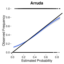
Figure 1: Scores and proportion of errors of the various predictive methods. Horizontal line represents the score of the trivial prediction $(1/3,1/3,1/3)$.

Table 3: Mean and total scores and their standard errors for the 1710 matches.

Score	BT	Arruda	Lee	$Mn-Dir_{1}$	$Mn-Dir_{2}$
	Mean Scores
Brier	0.635 (0.009)	0.616 (0.007)	0.629 (0.009)	0.624 (0.006)	0.628 (0.005)
Spherical$\times 10$	-6.077 (0.062)	-6.191 (0.055)	-6.112 (0.062)	-6.123 (0.048)	-6.098 (0.041)
Logarithmic	1.062 (0.014)	1.027 (0.011)	1.049 (0.013)	1.040 (0.009)	1.044 (0.008)
	Total Scores
Brier	1085.9 (14.9)	1053.2 (12.6)	1075.5 (14.9)	1067.59 (10.4)	1073.5 (8.8)
Spherical$\times 10$	-1039.2 (10.5)	-1058.7 (9.4)	-1046.9 (10.6)	-1047.0 (8.2)	-1042.7 (7.1)
Logarithmic	1816.4 (23.3)	1755.7 (18.0)	1793.6 (21.9)	1778.8 (15.5)	1785.2 (13.0)

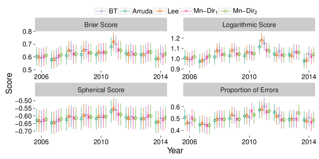
(a)

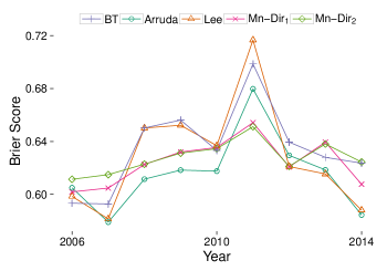
(b)

Figure 2: Means and standard errors of each measure of performance by year. Plot (b) shows the same information for the Brier scores, but without standard errors.

In order to formally check if all models have similar predictive power, we tested the hypotheses that all six models have the same average score. We did this by using a repeated measures ANOVA, a statistical test that takes into account the dependency between the observations (notice that each match is evaluated by each model). In order to perform multiple comparisons, we adjusted $p$-values so as to control the false discovery rate. All metrics presented significant differences at the level of significance of 5% ($p$-value $<0.01$ in all cases, see Table 4), except for the proportion of errors, where no difference was found. Post-hoc analyses are displayed in Table 5. Along with Table 3, one concludes that, for the Brier score, differences were found only between Mn-Dir₁ versus BT (the former had better performance), Mn-Dir₂ versus Arruda (the former had worse performance), and Arruda versus Lee (the former had better performance). For the spherical score, post-hoc analyses showed that the differences were found in Mn-Dir₂ versus Arruda (the former had worse performance) and BT versus Arruda (the former had worse performance). Finally, for the logarithmic score, post-hoc analyses showed that the differences were found in Mn-Dir₁ versus BT (the former had better performance), Mn-Dir₂ versus BT (the former had better performance), Lee versus Arruda (the former had worse performance), and Mn-Dir₂ versus Arruda (the former had worse performance).

These results therefore indicate that while the multinomial-Dirichlet models presented similar performances, they were better than BT and comparable to Lee. It is clear that the Arruda model presented the best performance, although the predictions from Mn-Dir₁ were not significantly different from it, according to all scoring rules. Hence, while BT lead to worse predictions than its competitors, Arruda was slightly better than some of its competitors, but roughly equivalent to Mn-Dir₁.

Table 4: ANOVA comparing the performance of all prediction models under the various scores.

Score	Factor	num. d.f.	den. d.f.	F-value	p-value
Brier	Intercept	1	8545.00	8423.04	$<$0.01∗
	Model	4	6836	5.15	$<$0.01∗
Spherical	Intercept	1	6836	14650.89	$<$0.01∗
	Model	4	6836	3.96	$<$0.01∗
Logarithmic	Intercept	1	6836	10876.28	$<$0.01∗
	Model	4	6836	6.76	$<$0.01∗
Proportion	Intercept	1	6836	2139.93	$<$0.01∗
of Errors	Model	4	6836	0.31	0.86

Table 5: Post-hoc analyses comparing the performance of all prediction models under the various scores.

Score	Comparison	Estimate	Std. Error	z-value	p-value
Brier	Arruda - BT	-0.02	0.00	-4.59	$<$0.01∗
	Lee - BT	-0.01	0.00	-1.47	0.24
	Mn-Dir1 - BT	-0.01	0.00	-2.58	0.04∗
	Mn-Dir2 - BT	-0.01	0.00	-1.75	0.16
	Lee - Arruda	0.01	0.00	3.12	0.01∗
	Mn-Dir1 - Arruda	0.01	0.00	2.01	0.11
	Mn-Dir2 - Arruda	0.01	0.00	2.84	0.02∗
	Mn-Dir1 - Lee	-0.00	0.00	-1.11	0.36
	Mn-Dir2 - Lee	-0.00	0.00	-0.28	0.79
	Mn-Dir2 - Mn-Dir1	0.00	0.00	0.83	0.48
Spherical	Arruda - BT	-0.01	0.00	-3.89	$<$0.01∗
	Lee - BT	-0.00	0.00	-1.54	0.23
	Mn-Dir1 - BT	-0.00	0.00	-1.55	0.23
	Mn-Dir2 - BT	-0.00	0.00	-0.69	0.57
	Lee - Arruda	0.01	0.00	2.35	0.06
	Mn-Dir1 - Arruda	0.01	0.00	2.34	0.06
	Mn-Dir2 - Arruda	0.01	0.00	3.20	0.01∗
	Mn-Dir1 - Lee	-0.00	0.00	-0.02	0.99
	Mn-Dir2 - Lee	0.00	0.00	0.85	0.59
	Mn-Dir2 - Mn-Dir1	0.00	0.00	0.87	0.59
Logarithmic	Arruda - BT	-0.04	0.01∗	-5.28	$<$0.01
	Lee - BT	-0.01	0.01	-1.99	0.08
	Mn-Dir1 - BT	-0.02	0.01	-3.28	0.01∗
	Mn-Dir2 - BT	-0.02	0.01	-2.72	0.02∗
	Lee - Arruda	0.02	0.01	3.29	0.01∗
	Mn-Dir1 - Arruda	0.01	0.01	2.01	0.08
	Mn-Dir2 - Arruda	0.02	0.01	2.57	0.03∗
	Mn-Dir1 - Lee	-0.01	0.01	-1.29	0.27
	Mn-Dir2 - Lee	-0.00	0.01	-0.73	0.54
	Mn-Dir2 - Mn-Dir1	0.00	0.01	0.56	0.59

We further illustrate this point in Figure 3(b), where the plots display the scores of each match for every couple of models considered. The plots show that all methods performed similarly, and that the multinomial-Dirichlet models are the ones that agreed the most.

(a)

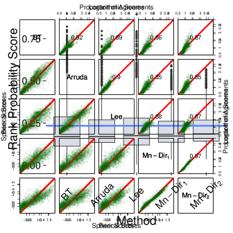
(b)

Figure 3: Pairwise comparisons of the various scores. (a): upper right plots display Logarithmic Scores; lower left plots display Brier Scores. (b): upper right plots display proportion of agreements between methods (i.e., proportion of times the conclusions are the same; see the Appendix); lower left plots display Spherical Scores. Lines represent

the identity $y=x$.

We also evaluated how reasonable were the predictions by assessing the calibration of the methods considered, i.e., by evaluating how often events which have assigned probability $p$ (for each $0<p<1$) happened (see the Appendix). If these observed proportions are close to $p$, one concludes that the methods are well-calibrated. The results are displayed in Figure 4. Because the Arruda and multinomial-Dirichlet models have curves that are close to the identity ($45^{\text{o}}$ line), we conclude that these methods are well-calibrated. On the other hand, BT and Lee seem to be poorly calibrated, over-estimating probabilities for the most frequent events.

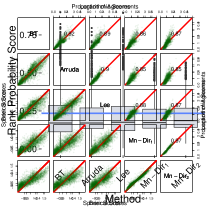
Figure 4: Calibration of the various predictive methods: estimates of occurrence frequency obtained by smoothing splines, with 95% confidence bands. Black line is the identity $y=x$.

3.1 Goodness of fit and information measures

We also evaluated the goodness of fit of each model by computing, for each team $t$, the following statistics:

$$e^{H}_{t}=\sum_{i\in H_{t}}\widehat{p}_{t,i}\ \ \ \mbox{ and }\ \ \ e^{A}_{t}=\sum_{i\in A_{t}}\widehat{p}_{t,i},$$

where $\widehat{p}_{t,i}$ is the estimated probability team $t$ wins the $i$-th match, $H_{t}$ is the set of matches team $t$ played as home team, and $A_{t}$ the set of matches team $t$ played away. We then computed a $\chi^{2}$ statistic

$$\chi^{2}_{o}=\sum_{t}\frac{(e^{H}_{t}-o^{H}_{t})^{2}}{e^{H}_{t}}+\frac{(e^{A}_{t}-o^{A}_{t})^{2}}{e^{A}_{t}},$$

where $o^{H}_{t}$ is the number of times team $t$ won playing home and $o^{A}_{t}$ is the number of times team $t$ won playing away. We then compared $\chi^{2}_{o}$ to a $\chi^{2}$ distribution with 40 degrees of freedom (twice the number of teams of each championship). Since we did not fit the Arruda model, this was the only goodness of fit measure we could compute.

The values of the statistics and their corresponding $p$-values are displayed in Table 6. Except for the BT model, all other methods presented reasonable goodness of fit, in particular, the multinomial-Dirichlet model 1, which presented the smaller chi-square statistics, thus indicating better fit.

Score	BT	Arruda	Lee	$Mn-Dir_{1}$	$Mn-Dir_{2}$
$\chi^{2}_{o}$	112.8	76.9	91.5	61.5	77.2
$p$-value	0.001	0.48	0.14	0.91	0.50

Table 6: Goodness of fit statistics for the models considered.

To have a deeper understanding about the probabilities given by each method, Figure 5 displays the estimated conditional probability that the home team wins assuming the match will not be a tie. All models assigned higher probabilities to the home team, showing that they captured the well-known fact known as home advantage, peculiar in football matches and other sport competitions (Pollard,, 1986; Clarke and Norman,, 1995; Nevill and Holder,, 1999).

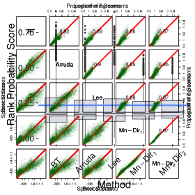
Figure 5: Conditional probability that the home team wins given there is no draw. Horizontal line indicates a 50% probability.

In order to check how informative the predictions provided by the six models were, we computed the entropy of their predictions. Recall that the entropy of a prediction $(p_{1},p_{2},p_{3})$ is given by $-\sum_{i=1}^{3}p_{i}\log{p_{i}}$. Figure 6 presents the box plots of the entropy of each prediction for all the studied models. Since the entropy values are smaller than 1.09, the plots show that the predictions were typically more informative than the trivial prediction. Nevertheless, all methods yielded similar entropies on average, that is, none of them provided more informative probabilities.

Figure 6: Entropy of the predictions of the various methods. Horizontal line represents the entropy of the trivial prediction $(1/3,1/3,1/3)$.

Summarizing our conclusions we may say that, for the matches considered in our analysis, all the studied models yielded better predictions than the trivial prediction. In particular the multinomial-Dirichlet models were well-calibrated, while the Lee model was not. Model Mn-Dir₁ presented the best goodness of fit statistic, while models Mn-Dir₂ and Arruda showed similar goodness-of-fit. About the scoring rules, while the Bradley-Terry model yielded worse predictions than its competitors according to all metrics, the Arruda model was the best one according to the three scoring rules considered in this work, but not in every championship. The scores of the predictions provided by the multinomial-Dirichlet models were, on average, similar to the scores of the Arruda model.

Therefore, we conclude that the multinomial-Dirichlet models are competitive with standard approaches.

4 Final Remarks

The benchmark models used in this work were chosen because of their wide popularity among football fans in Brazil, despite the availability of several other models in the literature. Among them, we can cite those that model the match as a stochastic process evolving in time (Dixon and Robinson,, 1998; Volf,, 2009; Titman et al.,, 2015), those allowing for the team performance parameters to change along the season (Rue and Salvesen,, 2000; Crowder et al.,, 2002; Owen,, 2011; Koopman and Lit,, 2015) and those modeling dependence between number of goals by means of bivariate count distributions (Dixon and Coles,, 1997; Karlis and Ntzoufras,, 2003; McHale and Scarf,, 2007, 2011). Contrary to the multinomial models we proposed, some of these approaches are able to answer several questions, for instance, they can estimate teams’ performance parameters allowing to rank the teams according to their offensive and defensive qualities, and can also predict the number of goals scored in a particular match.

Another critical difference between the benchmark and the multinomial models is that the latter are Bayesian, while the former are not. Not only the way they use past information is different (because of frequentist and Bayesian paradigms), but also the pieces of information used in the analysis (for example, the Arruda model uses results of the previous twelve months, including other championships, while multinomial models use only the previous matches of the current championship). One can argue that this may lead to unfair comparisons, which is true if the interest is on the inferential properties of the models; our interest, however, is on prediction only, the true purpose of all of these models. For prediction comparions, there is not even a need for a probabilistic model, as we have seen in the comparisons with the trivial prediction.

Nonetheless, when we are interested only on predicting the final outcome of future matches, the multinomial-Dirichlet models can perform equally well as their complex counterparts. The advantage of the first proposed model is that its predictions are obtained through simple calculations, without requiring numerical optimization procedures. The importance of such finding is directly related to the models usability in practice: professionals that use the mentioned benchmark models often say that a difficulty they face is that predictions may generate anger in football fans, which is then translated into distrust in subsequent predictions. Because of the complexity of some models, they find hard to explain to the lay user how the outcomes were predicted. This is where using simple models pays off: the first multinomial model yields results that are easy to explain because they only involve counts of losses, wins and draws, allowing one to offer simple explanations to football fans and journalists about the proposed predictions.

Our work also poses several questions about probabilistic prediction of sport events. In particular, based on the fact that the models have similar predictive power on average, one may ask: Is there an irreducible “randomness” or “degree of unpredictability” implicit in these events? Is this degree an indicator of how tight or leveled is the championship being studied?

A suggestion of future research is to answer these questions by considering more championships and models, and by comparing them using other scoring rules. We would also like to test other weighting methods in models $Mn-Dir_{1}$ and $Mn-Dir_{2}$ here proposed, and to evaluate their impact on the predictive power of the resulting predictions.

Another possible extension is to explore different prior distributions for the multinomial-Dirichlet models. In this work, we have predicted the second half of the season using a prior based on the first half. However, one can refine prior construction in order to enable first-half predictions. For instance, one can construct priors based on pre-season odds—e.g. odds for winning the championship, finishing in a given position— or on rankings of the teams—such as Elo rankings—provided by experts before the beginning of each championship and this is equivalent, one may say, to use the results of previous matches from a given time span.

Appendix: scoring rules and calibration

In this appendix we describe the scoring rules, how we computed the proportion of errors and the calibration measure used in the paper. Firstly we provide a definition of proper scoring rules with simple examples to illustrate some of them and afterwards we describe the criterion developed to verify if the models are calibrated.

One way to fairly rank predictive models is by using proper scoring rules, where the score may be interpreted as a numerical measure of how inaccurate a given probabilistic prediction was.

Formally, let $X$ be a random variable taking values in $\mathcal{X}=\{1,2,3\}$ indicating the outcome of the match, with 1 standing for home win, 2 for draw and 3 for away win. Moreover, let $P=(P_{1},P_{2},P_{3})$ denote one’s probabilistic prediction about $X$, i.e., $P$ lies in the 2-simplex set $\Delta_{2}=\{(p_{1},p_{2},p_{3}):p_{1}+p_{2}+p_{3}=1,\ p_{1},p_{2},p_{3}\geq 0\}$ (see Figure 7). A scoring rule is a function that assigns a real number (score) $S(x,P)$ to each $x\in\mathcal{X}$ and $P\in\Delta_{2}$ such that for any given $x$ in $\mathcal{X}$, the score $S(x,P)$ is minimized when $P$ is $(1,0,0)$, $(0,1,0)$ or $(0,0,1)$ depending if $x$ is 1, 2 or 3, respectively. The score $S(x,P)$ can be thought as a penalty to be paid when one assigns the probabilistic prediction $P$ and outcome $x$ occurs. Also, the “best” possible score (i.e., the smallest score value) is achieved when the probabilistic prediction for the outcome of the game is perfect. A scoring rule may also be defined to be such that a large value of the score indicates good forecasts.

Figure 7: Bi-dimensional simplex (gray surface): area of possible forecasts.

Although many functions can satisfy the above scoring rule definition, not all of them encourage honesty and accuracy when assigning a prediction to an event. Those that do enable a fair probabilistic assignment are named proper scoring rules (Lad,, 1996), which we describe in the sequence.

Consider a probabilistic prediction $P^{*}=(P_{1}^{*},P_{2}^{*},P_{3}^{*})$ for $X$. A proper scoring rule $S$ is a scoring rule such that the mean score value

$$E_{P^{*}}[S(X,P)]=\sum_{x=1}^{3}S(x,P)P^{*}_{x}$$

is minimized when $P=P^{*}$. In other words, if one announces $P$ as his probabilistic prediction and uses $S$ as scoring rule, the lowest expected penalty is obtained by reporting $P^{*}$, the model real uncertainty about $X$. Thus, the use of a proper scoring rule encourages the forecaster to announce $P^{*}$ (the correct one) as his probabilistic prediction rather than some other quantity.

In what follows, we describe in detail three proper scoring rules we use to assess the considered models. We also recall the concept of calibration and propose a way to measure the calibration degree of each model.

Brier Scoring Rule

Let $P=(P_{1},P_{2},P_{3})$ be a probabilistic prediction for $X$. The Brier score for a given outcome $x\in\{1,2,3\}$ is given by

$$S(x,P)=\sum_{i=1}^{3}\mathbb{I}(x=i)(1-P_{i})^{2}+\sum_{i=1}^{3}\mathbb{I}(x\neq i)P^{2}_{i},$$

where $\mathbb{I}$ is the indicator function.

We interpret the Brier score in the case where one of three mutually exclusive outcomes happens as in the case of a football match. The green surface in Figure 7 represents the 2-simplex, i.e., the set of points such that $p_{1}+p_{2}+p_{3}=1$ for non-negative values of $p_{1}$, $p_{2}$ and $p_{3}$. The triangle representing the simplex has sides of length $\sqrt{2}$ and its height is $\sqrt{6}/2$. Drawing a similar equilateral triangle with height 1 and sides $2\sqrt{3}/3$, it is possible to represent all points of the simplex. This new triangle is used to graphically display the forecast as an internal point because the sum of the distances of every point inside it to each side, representing the probability of each event, is always one. See Figure 8.

(a) Brier score, $d$, for victory of away team

(b) Normalized simplex: $p_{1}+p_{2}+p_{3}=1$

Figure 8: Standard (a) and normalized (b) simplexes.

The Brier score for the probabilistic prediction $P=(0.25,0.35,0.40)$ assuming the home team loses, is therefore given by $d^{2}=(0-0.25)^{2}+(0-0.35)^{2}+(1-0.40)^{2}=0.545$. On the other hand, the prediction $P=(0,0,1)$ achieves score zero, the minimum for this rule.

It is useful to consider the score of what we will call trivial prediction: $P=(1/3,1/3,1/3)$. This assessment will produce a Brier score of $2/3$, no matter what is the final result of the match, providing, thus, a threshold that a good model should consistently beat, meaning, for the Brier score, that the scores of its predictions should be smaller than $0.667$.

Logarithmic Scoring Rule

The logarithmic score is given by

$$S(x,P)=-\sum_{i=1}^{3}\mathbb{I}(x=i)\ln(P_{i}),$$

which is the negative log likelihood of the event that occurred.

The logarithmic score for the prediction $P=(0.25,0.35,0.40)$ when the home team loses is therefore $-\ln(0.4)\approx 0.91$. On the other hand, the prediction $P=(0,0,1)$ achieves score zero, once again the minimum of this rule. Moreover, for the logarithmic score, the trivial prediction gives a score of approximately $1.098$.

Spherical Scoring Rule

The spherical score is given by

$$S(x,P)=-\frac{1}{\sqrt{\sum_{i=1}^{3}P^{2}_{i}}}\sum_{i=1}^{3}\mathbb{I}(x=x_{i})P_{i},$$

which is the negative likelihood of the event that occurred, normalized by the square-root of the sum of the assigned squared probabilities.

The spherical score for the prediction $P=(0.25,0.35,0.40)$ assuming the home team loses, is given by $-0.4/\sqrt{0.25^{2}+0.35^{2}+0.40^{2}}\approx-0.68$. On the other hand, the prediction $P=(0,0,1)$ achieves score $-1$ instead and, for this rule, the trivial prediction results in a score of approximately $-0.577$.

Calibration and Proportion of Errors

Besides scoring rules, there are other criteria used to assess the quality of different predictions. Here we explore two of them.

The first one is the proportion of errors made by the model or assessor. This is simply the proportion of mistakes made when considering the highest probability assessment. More precisely, the proportion of errors of a sequence of probabilistic predictions for $n$ games, $P^{(1)},\ldots,P^{(n)}$ with $P^{(j)}=(P^{(j)}_{1},P^{(j)}_{2},P^{(j)}_{3})$, is defined by

$$\frac{1}{n}\sum_{j=1}^{n}\mathbb{I}\left(X_{j}\neq\arg\max_{x\in\{1,2,3\}}P^{(j)}_{x}\right),$$

where $X_{j}$ is the outcome of the $j$-th match.

The second concept we use is that of calibration (Dawid,, 1982). Probability assertions are said to be well calibrated at the level of probability $p$ if the observed proportion of all propositions that are assessed with probability $p$ equals $p$.

Because we typically do not have several predictions with the same assigned probability $p$, we obtain a plot by smoothing (i.e., regressing) the indicator function of whether a given result happened as a function of the probability assigned for that result. That is, we estimate the probability that an event occurs given its assigned probability. The smoothing was done via smoothing splines (Wahba,, 1990), with tuning parameters chosen by cross-validation.

References

- Agresti, (2010) Agresti, A. (2010). Analysis of ordinal categorical data, volume 656. John Wiley & Sons.
- Bernardo and Smith, (1994) Bernardo, J. M. and Smith, A. F. (1994). Bayesian Theory. Wiley.
- Bradley and Terry, (1952) Bradley, R. A. and Terry, M. E. (1952). Rank analysis of incomplete block designs: I. the method of paired comparisons. Biometrika, 39(3/4):324–345.
- Brier, (1950) Brier, G. W. (1950). Verification of forecasts expressed in terms of probability. Monthly weather review, 78(1):1–3.
- Brillinger, (2008) Brillinger, D. R. (2008). Modelling game outcomes of the Brazilian 2006 Series A Championship as ordinal-valued. Brazilian Journal of Probability and Statistics, pages 89–104.
- Brillinger, (2009) Brillinger, D. R. (2009). An analysis of Chinese Super League partial results. Science in China Series A: Mathematics, 52(6):1139–1151.
- Clarke and Norman, (1995) Clarke, S. R. and Norman, J. M. (1995). Home ground advantage of individual clubs in English soccer. The Statistician, pages 509–521.
- Constantinou et al., (2012) Constantinou, A. C., Fenton, N. E., et al. (2012). Solving the problem of inadequate scoring rules for assessing probabilistic football forecast models. Journal of Quantitative Analysis in Sports, 8(1):1559–0410.
- Crowder et al., (2002) Crowder, M., Dixon, M., Ledford, A., and Robinson, M. (2002). Dynamic modelling and prediction of English Football League matches for betting. Journal of the Royal Statistical Society: Series D (The Statistician), 51(2):157–168.
- Davidson, (1970) Davidson, R. R. (1970). On extending the Bradley-Terry model to accommodate ties in paired comparison experiments. Journal of the American Statistical Association, 65(329):317–328.
- Davidson and Beaver, (1977) Davidson, R. R. and Beaver, R. J. (1977). On extending the Bradley-Terry model to incorporate within-pair order effects. Biometrics, pages 693–702.
- Dawid, (1982) Dawid, A. P. (1982). The well-calibrated Bayesian. Journal of the American Statistical Association, 77(379):605–610.
- de Arruda, (2000) de Arruda, M. L. (2000). Poisson, Bayes, futebol e de Finetti. Master’s thesis, University of São Paulo, São Paulo, Brazil.
- de Arruda, (2015) de Arruda, M. L. (2015). Chance de gol. http://www.chancedegol.com.br. [Online; accessed 11-September-2015].
- Dixon and Robinson, (1998) Dixon, M. and Robinson, M. (1998). A birth process model for association football matches. Journal of the Royal Statistical Society: Series D (The Statistician), 47(3):523–538.
- Dixon and Coles, (1997) Dixon, M. J. and Coles, S. G. (1997). Modelling association football scores and inefficiencies in the football betting market. Journal of the Royal Statistical Society: Series C (Applied Statistics), 46(2):265–280.
- Forrest and Simmons, (2000) Forrest, D. and Simmons, R. (2000). Focus on sport: Making up the results: the work of the football pools panel, 1963-1997. Journal of the Royal Statistical Society: Series D (The Statistician), 49(2):253–260.
- Genest and Zidek, (1986) Genest, C. and Zidek, J. V. (1986). Combining probability distributions: A critique and an annotated bibliography. Statistical Science, 1(1):114–135.
- GMEE, (2015) GMEE (2015). Previsão esportiva. http://www.previsaoesportiva.com.br. [Online; accessed 11-September-2015].
- Goddard, (2005) Goddard, J. (2005). Regression models for forecasting goals and match results in association football. International Journal of forecasting, 21(2):331–340.
- Good et al., (1966) Good, I. J., Hacking, I., Jeffrey, R., and Törnebohm, H. (1966). The estimation of probabilities: An essay on modern Bayesian methods.
- Holgate, (1964) Holgate, P. (1964). Estimation for the bivariate Poisson distribution. Biometrika, 51(1-2):241–287.
- Karlis and Ntzoufras, (2003) Karlis, D. and Ntzoufras, I. (2003). Analysis of sports data by using bivariate Poisson models. Journal of the Royal Statistical Society: Series D (The Statistician), 52(3):381–393.
- Koning, (2000) Koning, R. H. (2000). Balance in competition in Dutch soccer. Journal of the Royal Statistical Society: Series D (The Statistician), 49(3):419–431.
- Koopman and Lit, (2015) Koopman, S. J. and Lit, R. (2015). A dynamic bivariate Poisson model for analysing and forecasting match results in the english premier league. Journal of the Royal Statistical Society: Series A (Statistics in Society), 178(1):167–186.
- Lad, (1996) Lad, F. (1996). Operational Subjective Statistical Methods: a mathematical, philosophical, and historical introduction, volume 315. Wiley-Interscience.
- Lee, (1997) Lee, A. J. (1997). Modeling scores in the Premier League: is Manchester United really the best? Chance, 10(1):15–19.
- Lehrer, (1983) Lehrer, K. (1983). Rationality as weighted averaging. Synthese, 57:283–295.
- Maher, (1982) Maher, M. J. (1982). Modelling association football scores. Statistica Neerlandica, 36(3):109–118.
- McConway, (1981) McConway, K. J. (1981). Marginalization and linear opinion polls. Journal of the American Statistical Association, 76:410–414.
- McHale and Scarf, (2007) McHale, I. and Scarf, P. (2007). Modelling soccer matches using bivariate discrete distributions with general dependence structure. Statistica Neerlandica, 61(4):432–445.
- McHale and Scarf, (2011) McHale, I. and Scarf, P. (2011). Modelling the dependence of goals scored by opposing teams in international soccer matches. Statistical Modelling, 11(3):219–236.
- Nevill and Holder, (1999) Nevill, A. M. and Holder, R. L. (1999). Home advantage in sport. Sports Medicine, 28(4):221–236.
- Owen, (2011) Owen, A. (2011). Dynamic Bayesian forecasting models of football match outcomes with estimation of the evolution variance parameter. IMA Journal of Management Mathematics, 22(2):99–113.
- Pollard, (1986) Pollard, R. (1986). Home advantage in soccer: A retrospective analysis. Journal of Sports Sciences, 4(3):237–248.
- R Core Team, (2015) R Core Team (2015). R: A language and environment for statistical computing. Vienna, Austria: R Foundation for Statistical Computing; 2014. R Foundation for Statistical Computing.
- Rue and Salvesen, (2000) Rue, H. and Salvesen, O. (2000). Prediction and retrospective analysis of soccer matches in a league. Journal of the Royal Statistical Society: Series D (The Statistician), 49(3):399–418.
- Stone, (1961) Stone, M. (1961). The opinion pool. Annals of Mathematical Statistics, 32:1339–1342.
- Titman et al., (2015) Titman, A., Costain, D., Ridall, P., and Gregory, K. (2015). Joint modelling of goals and bookings in association football. Journal of the Royal Statistical Society: Series A (Statistics in Society), 178(3):659–683.
- Van Rossum and Drake Jr, (2014) Van Rossum, G. and Drake Jr, F. L. (2014). The python language reference.
- Volf, (2009) Volf, P. (2009). A random point process model for the score in sport matches. IMA Journal of Management Mathematics, 20(2):121–131.
- Wahba, (1990) Wahba, G. (1990). Spline models for observational data, volume 59. Siam.
- Yan, (2016) Yan, T. (2016). Ranking in the generalized Bradley–Terry models when the strong connection condition fails. Communications in Statistics-Theory and Methods, 45(2):340–353.