Recognising Axionic Dark Matter by Compton and de-Broglie Scale Modulation of Pulsar Timing.

Abstract

Light Axionic Dark Matter, motivated by string theory, is increasingly favored for the “no-WIMP era”. Galaxy formation is suppressed below a Jeans scale, of $\simeq 10^{8}M_{\odot}$ by setting the axion mass to, $m_{B}\sim 10^{-22}$eV, and the large dark cores of dwarf galaxies are explained as solitons on the de-Broglie scale. This is persuasive, but detection of the inherent scalar field oscillation at the Compton frequency, $\omega_{B}=(2.5{\rm\,months})^{-1}(m_{B}/10^{-22}eV)$, would be definitive. By evolving the coupled Schrödinger-Poisson equation for a Bose-Einstein condensate, we predict the dark matter is fully modulated by de-Broglie interference, with a dense soliton core of size $\simeq 150pc$, at the Galactic center. The oscillating field pressure induces General Relativistic time dilation in proportion to the local dark matter density and pulsars within this dense core have detectably large timing residuals, of $\simeq 400nsec/(m_{B}/10^{-22}eV)$. This is encouraging as many new pulsars should be discovered near the Galactic center with planned radio surveys. More generally, over the whole Galaxy, differences in dark matter density between pairs of pulsars imprints a pairwise Galactocentric signature that can be distinguished from an isotropic gravitational wave background.

I Introduction

Axions are a compelling choice for extending the standard model in particle physics, generating oscillating dark matter with symmetry broken by the misalignment mechanism Preskill:1982cy ; Abbott:1982af ; Dine:1982ah . Such fields are generic to string theory, arising from dynamical compactification to 4 space-time dimensions, so that multiple stabilized, complex scalar fields naturally appear (e. g. Ref Svrcek:2006yi ). Such an axion is effectively massless until the Universe cools below some critical temperature, and rolls down a small non-pertubatively generated potential, oscillating about the minimum, corresponding to a coherent zero-momentum axion. It is argued that very light axions are very natural in this context Hui:2016ltb and furthermore, in a ”string theory landscape”, the cosmological constant may also be naturally small and accompanied by correspondingly very light scalar bosons Tye:2016jzi .

Axion oscillation generates field pressure at frequency $2m_{B}$, with static energy density to leading order that is coherent below the de-Broglie scale. At a certain scale, self-gravity is balanced by field pressure, yielding a static, centrally located density peak, or soliton. The soliton scale depends on the gravitational potential corresponding to only 150 pc for the Milky Way Schive2014 . Throughout the Galaxy, gravity is balanced by the axion pressure forming density “granules” of similar scale to the soliton from interference of many large-amplitude de Broglie waves which are unstable, regenerating themselves with a lifetime of about 1 Myr for our Galaxy Schive2014b .

Khmeinitsky and Rubakov (2013) made the very interesting observation that the field pressure oscillations on the Compton scale leads to an oscillating gravitational potential that can affect pulsar timing measurements Khmeinitsky:2013lxt . They assume a constant local dark matter density so pulsar timing and our Earth clock will be affected in the same way, with a net relative timing modulation from the phase difference that will be very challenging to detect. However, we show here that a much stronger signal is expected towards the Galactic center, in and around the solitonic core that we predict for light axionic Dark Matter. This additional de-Broglie structure is absent in Khmeinitsky:2013lxt , which predates the first simulations of galaxies in this context, Schive2014 . We show this greatly enhances the expected pulsar timing modulation by 2-3 orders of magnitude within the central Kiloparsec of our Galaxy, for our favoured axion mass ($0.8\times 10^{-22}eV$, Schive2014 ), well within the current bounds of detectability, providing a direct, practical test for Axions.

Here we calculate this additional de-Broglie effect self consistently, by including our simulated halo structure. This is an important feature that is absent in Ref Khmeinitsky:2013lxt , which if observed would directly support light bosonic dark matter. The parameters assumed are: Hubble constant $H_{0}=70$ km/sec/Mpc with critical density $\rho_{c}=6\rm{\,GeV\,m}^{-3}$, and present dark matter density $\rho_{0}=1.5\rm{\,GeV\,m}^{-3}$.

II Compton Scale Pressure Oscillation and Pulsar Timing

For a single real scalar field $\phi$ with harmonic potential oscillation: $\phi({\bf x},t)=A({\bf x})\cos(m_{B}\,t+\alpha({\bf x}))$, where $m_{B}$ is the associated boson mass. We let $\Re[\psi]\cos(m_{B}t)+\Im[\psi]\sin(m_{B}t)\equiv m_{B}^{1/2}\phi$ to relate $\phi$ to the complex wave function of Schroedinger’s equation, so $m_{B}^{1/2}A$ and $\alpha$ are the amplitude and phase of $\psi$, respectively. From the energy-momentum tensor one obtains an oscillating pressure $p({\bf x},t)=-\frac{1}{2}m_{B}^{2}A^{2}\cos{(\omega\,t+2\alpha)}$ with frequency $\omega=2\pi\nu=2m_{B}$. These oscillations are usually neglected as the average pressure over the period is zero. However, at the Compton scale of interest here, the oscillating scalar field generates an oscillating gravitational potential in proportion to the local mass density Khmeinitsky:2013lxt . All clocks are modulated by such an oscillating field, including Earth clocks and Pulsars.

It is customary to write the time dependent part of the time residuals as the relative frequency shift of the pulse

$$\delta t(t)=-\int_{0}^{t}\frac{\nu(t^{\prime})-\nu_{0}}{\nu_{0}}\,dt^{\prime},$$ (1)

where $\nu(t^{\prime})$ is the pulse frequency at the detector, emitted at a distance $D$ at the time $t^{\prime}=t-D/c$, and $\nu_{0}$ is the pulsar emission frequency. To rewrite the Eq. (1) in terms of the oscillating gravitational potential we consider the linearized Einstein equations in the Newtonian gauge with two potentials $h_{00}=2\Phi$ and $h_{ij}=-2\Psi\delta_{ij}$. Then, the frequency shift is Gorbunov2011

$$\frac{\nu(t)-\nu_{0}}{\nu_{0}}\approx\Psi(\mathbf{x_{p}},0)-\Psi(\mathbf{x},t).$$ (2)

where $\bf{x_{p}}$ is the source position. Thus, to compute the frequency shift we need only consider the oscillating contribution to $\Psi$. Therefore, from the spatial components of the linearized Einstein equations the amplitude is:

$$\Psi_{c}({\bf x})=\pi\frac{G\rho_{DM}({\bf x})}{m_{B}^{2}}.$$ (3)

We stress the amplitude of the oscillation will vary over the Galaxy density with large de-Broglie scale modulations about the mean which is close to the Navarro-Frenk-White (NFW) profile NFW1996 (see Figure 1).

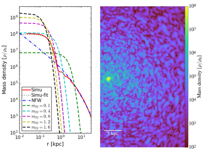
Figure 1: The left panel shows predicted soliton profiles for a range of $m_{B}$ (dashed curves), including the profile of a massive simulated halo of $10^{11}M_{\odot}$ (solid red curve), corresponding to the simulation on the right (using the yt package Turk2011 ), where the granular de-Broglie scale structure is visible on all scales, including the dense central soliton. Also indicated is an NFW profile (blue dashed curve) that fits well the azimuthally averaged galaxy profile (solid red curve).

Plugging eqs. (2) and (3) into (1), we obtain the time-dependent part of the time residuals for the $i-th$ pulsar with respect to the average signal ($\Delta t_{i}=\delta t_{i}-<\delta t_{i}>$):

$$\Delta t_{i}(t) = \frac{1}{\omega}\biggl{[}\Psi({\bf x_{i}})\sin\left(\omega(t-\frac{D_{i}}{c})+2\alpha_{i}\right)-$$ (4)

$$- \Psi({\bf x_{e}})\sin\left(\omega t+2\alpha_{e}\right)\biggr{]},$$

where $\alpha_{i}\equiv\alpha({\bf x_{i}})$ and $D_{i}$ are the phase and the pulsar distance and $\alpha_{e}\equiv\alpha({\bf x_{e}})$ is the phase of the Earth clock, hence cancellation of timing residuals is possible, and when pairs of clocks/pulsars are maximally out of phase their relative timing residual is enhanced, see Figure 2.

The timing differences between two well separated pulsars will be enhanced by the modulation of the axion density field on the de-Broglie scale throughout the Galaxy, as shown in Figures 1& 2, as the density structure is predicted by our simulations to be fully modulated on the de-Broglie scale.

III de-Broglie Scale Galactic Structure

Bosonic Dark Matter, such as Axions, if sufficiently light can satisfy the ground state condition, where the de-Broglie wavelength exceeds the mean particle separation set by the density of dark matter. This is simply described by a coupled Schroedinger-Poisson equation, analogous to the Gross-Pitaeviski equations for a Bose-Einstein condensate. Expressed in comoving coordinates we have:

$$\biggl{[}i\frac{\partial}{\partial\tau}+\frac{\nabla^{2}}{2}-aV\biggr{]}\psi=0\,,$$ (5)

$$\nabla^{2}V=4\pi(|\psi|^{2}-1)\,,$$ (6)

where $\psi$ is the wave function, $V$ is the gravitation potential and $a$ is the cosmological scale factor. The system is normalized to the time scale $d\tau=\chi^{1/2}a^{-2}dt$, and to the scale length $\xi=\chi^{1/4}(m_{B}/\hbar)^{1/2}{\mathbf{x}}$, where $\chi=\frac{3}{2}H_{0}^{2}\Omega_{0}$ where $\Omega_{0}$ is the current density parameter Widrow1993 .

The simplest “Fuzzy Dark Matter” case of no self-interaction was first advocated by Hu et al. Hu2000 for which the boson mass is the only free parameter, with further work in relation to dwarf galaxies Marsh2014 ; Bozek2015 . New Cosmological simulations in this context, dubbed $\psi_{DM}$, by Schive2014 have uncovered rich non-linear structure by solving the above equation, evolved from an initial standard power spectrum truncated at the inherent Jeans scale. A solitonic core forms within each virialized halo, naturally explaining dark matter dominated cores of dwarf spheroidal galaxies Schive2014 . The central soliton is surrounded by an extended halo with “ granular” texture on the de-Broglie scale in Figure 1, which on average follows the NFW form outside the soliton Schive2014 ; Schive2014b , as seen in Figure 1. This agreement can be understood because the pressure from the uncertainty principle is limited to the de-Broglie radius, beyond which is it negligible and behaves as collisionless CDM.

The identification of the centrally stable soliton with the large cores of dSph galaxies has allowed the boson mass to be estimated with little model dependence Schive2014 ; Schive2014b ; Zhang2017 . The best constraint comes form the well studied Fornax dwarf spheroidal (dSph), with an estimated halo mass is $4\times 10^{9}M_{\odot}$, yielding the soliton peak density is $2$ GeV cm^-3 and core width $1$ kpc Schive2014 and $m_{B}=0.8\times 10^{-22}$ eV, with somewhat larger $m_{B}$ derived using dSph galaxies from the SDSS survey Calabrese2016 . This allows us to predict the soliton scale expected for the Milky Way by using the scaling between Halo mass and Soliton mass scaling law: $\rho_{peak}\propto M_{halo}^{4/3}$ and $r_{c}\propto M_{halo}^{-1/3}$ derived from simulations Schive2014 ; Schive2014b , which for our Galaxy with a mass $M_{halo}^{MW}=2\times 10^{12}M_{\odot}$ Portail2017 , implies a MW soliton peak density $\rho_{peak}^{MW}=8\times 10^{3}$ GeV cm^-3 and soliton core width $r_{c}^{MW}=120$ pc (Figure 1). The Milky Way halo is generally taken to have a dark matter density $0.3$ GeV cm^-3 in the solar neighborhood, with recent careful studies by Portail et al. Portail2017 and Sivertsson et al (2017) , revising upward this figure to $0.5--0.6$ GeV cm^-3 . Our predicted soliton for our Galaxy ranges over $4-8\times 10^{3}$ and from Eq.(5) above, we have $\Delta t=\pi G\rho_{DM}/2m_{B}^{3}=(0.7-1.4)\times 10^{-27}m_{B}^{-3}$ sec^-2. Since $m_{B}=1.5\times 10^{-7}$ sec^-1, we arrive at $\Delta t=200-400$ nsec; this $\Delta t$ is within the reach of current pulsar time arrays. The central soliton then provides approximately two orders of magnitude enhancement of the DM density within $r\lesssim 100pc$, dominating the Earth clock and pulsars elsewhere in the galaxy as shown in Figure 2 (top left). For pairs of pulsars within this soliton region, separated by more than the Compton wavelength of ($>pc$ scale), the combined amplitude cancels or adds constructively to to a factor of two, as shown in Figure 2. The above assumes $m_{B}=10^{-22}$ eV, but allowing this to vary we have $\rho\propto m_{B}^{2}$ and $r_{c}\propto m_{B}^{-1}$, and thus $\Delta t\propto m_{B}^{-1}$, increasing the soliton density becomes higher, but the core radius is reduced.

IV Pairwise Timing Amplitudes

It is important to appreciate that all clocks are modulated within an oscillating scalar field including Earth clocks and so in practice we can work only with relative timing residuals, either between pairs of pulsars or between any pulsar and a time standard based on precise Earth clocks. The ticks of an individual clock are cyclically slowed and increased at the Compton frequency, with a magnitude that is proportional to the mass density of the scalar field local to each pulsar, where the ”amplitude” of this effect is the time difference induced by Eq. 3. In practice, pulsar timing measurements are typically averaged over a sizeable number of pulses on a relatively short timescale of hours and this rate is then compared on longer timescales, a practice that is well suited to the larger than monthly Compton frequency modulation that we seek, set by the axion mass. This timescale, note, is unaffected by the slow changes in structure on the de-Broglie scale of $\simeq 1Myr$ that set the amplitude of the timing residual for a given axion mass via equation 3.

The timing amplitude of any such modulation is determined by the de-Broglie scale density modulation which is largest for a pulsars within the central soliton and also when the pulsars are spatially located such that they are out of phase relative to the Compton frequency. In general this phase difference means that for any given pair of pulsars, for which the local Axion density is equal, range in relative amplitude from zero to double the amplitude of each separately, as shown by the blue shaded area in Figure 2. Furthermore, for well separated pulsars (on a scale greater then the de-Broglie scale) the timing amplitude range can be enhanced by another factor of two because of the de-Broglie scale interference that fully modulates the local density about the mean level, shown in Figure 2.

Ideally, the relative pulsar timing may not have to rely on being referred to any Earth clock for simultaneous observations of different pulsars through the same telescope, or for telescopes that are highly synchronous, with the advantage that any vagaries in precision of Earth clocks cancel. So here we calculate the relative timing amplitudes for pairs of pulsars $S(t)$:

$$S(t) = \Delta t_{1}(t)-\Delta t_{2}(t)=\frac{1}{\omega}\biggl{[}\Psi({\bf x_{1}})\sin\left(\omega t+\alpha^{\prime}_{1}\right)-$$ (7)

$$- \Psi({\bf x_{2}})\sin\left(\omega t+\alpha^{\prime}_{2}\right)\biggr{]},$$

where we have defined $\alpha^{\prime}_{i}=2\alpha_{i}-\frac{\omega D_{i}}{c}$. To illustrate this difference we calculate the relative timing signal in Figure 2 between local pulsars, and pulsars close to the Galactic center at a radius of 50 and 500 pc, fixing the boson mass to $m_{B}\sim 0.8\times 10^{-22}$ eV. In this case, the relative timing amplitude is dominated by the pulsar closer to the Galactic center and it can reach an amplitude of the order of 600 ns. While taking the pulsars at approximately the same distance from the Galactic center, the relative timing amplitude signal strongly depends on the phase of the pulse, canceling when the signals as seen from Earth are in phase.

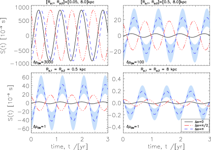
Figure 2: Predicted timing signal between pulsar pairs, for a light scalar field of $m_{B}\sim 0.8\times 10^{-22}$ eV. In the top panels the relative timing signal between local pulsars at $8$ kpc, and pulsars close to the Galactic center at a radius of 50 and 500 pc. In the bottom left and right panels both members of the pair are located at the same Galactocentric radius of $0.5$ and $8$ kpc, with relative phases chosen indicated in the inset box, bottom right, illustrating the signal can cancel in such cases. The shaded regions indicate how the density modulation on the de-Broglie scale can enhance or diminish the pairwise relative timing signal.

For convenience, we define ratio of the DM density at the locations of the two pulsars as

$$\delta\rho_{DM}=\left(\frac{\Psi({\bf x_{1}})}{\Psi({\bf x_{2}})}\right)=\frac{\rho_{DM}({\bf x_{1}})}{\rho_{DM}({\bf x_{2}})}.$$ (8)

To estimate the detectability of forthcoming pulsar timing arrays to the Axion oscillation we compute the average square signal over all the phases

$$\sqrt{\langle S^{2}(t)\rangle}=\frac{\sqrt{2}}{2\omega}\sqrt{\Psi({\bf x_{1}})^{2}+\Psi({\bf x_{2}})^{2}},$$ (9)

and relate it to the GW strain, and since the $\Psi({\bf x})$ amplitude of the oscillation only depends on the Axion density we can always re-write $\Psi({\bf x_{2}})$ in term of $\Psi({\bf x_{1}})$

$$h_{c}=\frac{\sqrt{6}}{2}\Psi({\bf x_{2}})\sqrt{1+\delta\rho_{DM}^{2}}.$$ (10)

We compute the characteristic amplitude shown in Figure 3, highlighting the relatively strong signal expected for pulsars within $\sim 0.5$ kpc of the Galactic center, We also over-plot the confidence regions for the current results from Pulsar Timing Array (PTA), Parkes Pulsar Timing Array (PPTA), Square Kilometre Array (SKA) experiments to allow a direct comparison with expected sensitivities of these new surveys Sesana2010 , where even one such central pulsar can provide a sufficient timing residual to test for the presence of light axionic dark matter.

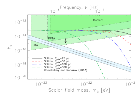
Figure 3: Characteristic strain measured between pairs of pulsars, with Galactocentric radii chosen as in Figure 2 and compared with the expected sensitivities from the current and forthcoming PTA experiments (adapted from Sesana2010 ; Khmeinitsky:2013lxt ), with the corresponding oscillation frequency shown above. We highlight the relatively high signal strength we calculate for pulsars within the Galactic soliton region as a function of Axion mass in a series of curves, demonstrating that this signal is already detectable for central Galactic pulsars. For comparison, the diagonal dotted line is the prediction obtained by Khmeinitsky:2013lxt for local pulsars, assuming a smooth density distribution, with the blue shaded region representing the wider range we predict that includes our de-Broglie scale DM density modulation. The local upper limit obtained by Porayko2014 is also shown (black square with arrow).

V Discussion and Conclusions

We have considered Compton and de-Broglie scale modulations within the Axionic interpretation of dark matter and examined their combined effect on Pulsar timing. For our Galaxy we estimate the de-Broglie scale is approximately 100 times larger than the Compton scale, corresponding to $\simeq 150pc$ for the Milky Way, with the favoured axion mass of $m_{B}\simeq 10^{-22}eV$. Within virialized halos our simulations reveal that the density distribution is fully modulated on the de-Broglie scale, as shown in Figure 1, with a dense soliton at the center of radius $\simeq 150pc$ where the pulsar timing effect is strong. Compton oscillation will be coherent within de-Broglie sized patches, becoming unrelated on larger scales. We have made self consistent predictions for pulsar timing residuals including this spatial dependence revealed in our $\psi_{DM}$ simulations Schive2014 .

The de-Broglie interference is most conspicuous by the formation of central soliton on the de-Broglie scale, representing a stable, time-independent ground state, where the pulsar timing residuals are expected to be 2-3 orders of magnitude higher than those imprinted on local pulsars, due to the relatively high central density of the soliton, that much exceeds in density a corresponding NFW profile. Such central millisecond pulsars are expected in large numbers within the bulge and near the galactic center Figer2004 ; Calore2016 , and can account for the GeV gamma-ray excess Abazaijan2011 ; Abazaijan2014 and are being searched with some success Johnston2006 ; Deneva2009 . Detection will be compromised within the inner 100 pc where the high plasma density is high and the ISM contains small scale irregularities, causing dispersion of pulse arrival time and pulse smearing, although “corridors” of lower scattering may be evident Macquart2015 ; Schnitzeler2016 . The smearing is a low-pass filter making millisecond pulsars undetectable at low frequency, but decreases rapidly at high frequency ($<$10Ghz) as $\nu^{-4}$. Blind searches are not yet very practical at these frequencies with single dishes and the pulse amplitude is typically relatively weak, but soon the SKA will be efficiently capable of detecting the putative population of central millisecond pulsars and comprehensive searches are already underway Macquart2015 ; Bhakta2017 .

In terms of the central potential of the Galaxy, the stellar bar dominates, but the signature of this soliton feature is expected dynamically on a scale of $\lesssim 150/m_{B}$ pc, which lies between the scale length of the stellar bulge (1 kpc) and the smaller pc scale region of influence of the central Milky Way black hole. Careful dynamical modeling by Portail et al. Portail2017 has recently uncovered a central shortfall of $2\times 10^{9}M_{\odot}$ of ”missing matter” which may help account for the 100 km/s motion of stars within the central $\simeq 120$ pc of the galaxy Kruijssen2015 ; Henshaw2016 ; Schonrich2015 and which we aim to examine in the context of the near spherical soliton potential that we predict here.

By using pulsars spread over a wide range of Galactocentric radius we may detect the radial dependence of pulsar timing ampliude on the dark matter density, beyond current limits claimed in Porayko2014 and pulsar binary resonance Blas2017 . This dependence helps distinguish the monotone Compton scale modulation we seek from an isotropic, stochastic GW background that has broad band variance. In making such pairwise measurements we have stressed that only relative timing variations can be detected as all clocks are modulated on the same Compton frequency scale including Earth clocks. Furthermore, we can anticipate a relatively large variance of such timing residuals because of the large density modulation from de-Broglie scale interference. The timing residual will absent for Pulsars at density minima but can be enhanced by 100% for pairs that lie near density maxima and located out of phase with respect to the Compton oscillation. This means that we cannot rely on only one pair of pulsars when assessing the presence of this Compton frequency, but must examine an ensemble to average over the combined Compton and de-Broglie modulation for a statistical detection.

For pulsars that may be detected in local dwarf spheroidal galaxies where the entire visible content lies within a solitonic core Schive2014 , the timescale is set by $m_{B}$ but the timing amplitude will by lower, set by the soliton density which scales as $M_{halo}^{4/3}$ Schive2014b , about a factor of $10^{-3}$ smaller than for the Galactic center, close to the current PTA capability limit.

IDM acknowledges support from University of the Basque Country program “Convocatoria de contratación para la especialización de personal investigador doctor en la UPV/EHU 2015”, and from the Spanish Ministerio de Economía y Competitividad through research project FIS2010-15492, and the Basque Government research project IT-956-16. RL is supported by the Spanish Ministry of Economy and Competitiveness through research projects FIS2010-15492 and Consolider EPI CSD2010-00064, and the University of the Basque Country program UFI 11/55. IDM and RL also acknowledges the support from the COST Action CA1511 Cosmology and Astrophysics Network for Theoretical Advances and Training Actions (CANTATA). TJB acknowledges generous hospitality from the Institute for Advanced Studies in Hong Kong and helpful conversations with Nick Kaiser and Kfir Blum. SHHT is supported by the CRF Grant HKUST4/CRF/13G and the GRF 16305414 issued by the Research Grants Council (RGC) of the Government of the Hong Kong SAR. The GPU cluster donated by Chipbond Technology Corporation, with which this work is conducted, is acknowledged. This work is supported in part by the National Science Council of Taiwan under the grants NSC100-2112-M-002-018-MY3 and NSC99-2112-M-002-009-MY3.

References

- (1) J. Preskill, M. B. Wise and F. Wilczek, Phys. Lett. 120B, 127 (1983).
- (2) L. F. Abbott and P. Sikivie, Phys. Lett. 120B, 133 (1983).
- (3) M. Dine and W. Fischler, Phys. Lett. 120B, 137 (1983).
- (4) P. Svrcek and E. Witten, JHEP 0606, 051 (2006)
- (5) L. Hui, J. P. Ostriker, S. Tremaine and E. Witten, Phys. Rev. D 95, no. 4, 043541 (2017)
- (6) S.-H. H. Tye and S. S. C. Wong, arXiv:1611.05786 [hep-th] (2016).
- (7) A. Khmelnitsky and V. Rubakov, JCAP, 2 , 019 (2014).
- (8) D. S. Gorbunov and V. A.Rubakov, Introduction to thetheory of the early universe, World Scientific Pub. Co., Singapore; Hackensack, N.J., (2011).
- (9) J. F. Navarro, C. S. Frenk, & S. D. M. White ApJ, 462, 563-575 (1996).
- (10) M.J. Turk, B. D. Smith, J. S. Oishi, S. Skory, S. W. Skillman, T. Abel, M. L. Norman, ApJ, 192, 1 (2011)
- (11) L.M. Widrow, N. Kaiser, ApJ, 416, 71 (1993).
- (12) W. Hu, R. Barkana, & A. Gruzinov Phys. Rev. Lett., 85, 1158 (2000).
- (13) D. J. E. Marsh, J. Silk, MNRAS, 437, 3, 2652-2663 (2014).
- (14) B. Bozek, D. J. E. Marsh, J. Silk, R. F.G. Wyse MNRAS, 450, 1, 209-222 (2015)
- (15) Hsi-Yu Schive, T. Chiueh, T. Broadhurst, Nature Physics, 10, 7, 496-499 (2014).
- (16) T-P. Woo, & T. Chiueh, ApJ, 697, 850-861 (2009).
- (17) Hsi-Yu Schive, M-H Liao, T-P Woo, S-K Wong, T. Chiueh, T. Broadhurst, and W-Y. Pauchy Hwang Phys. Rev. Lett., 113, 261302 (2014).
- (18) U-H Zhang, T. Chiueh, arXiv:17020.7065 (2017)
- (19) E. Calabrese, D. N. Spergel, MNRAS, 460, 4397 (2016).
- (20) M. Portail, O. Gerhard, C. Wegg, M. Ness, MNRAS, 465, 2, 1621-1644 (2017).
- (21) S. Sivertsson, H. Silverwood, J. I. Read, G. Bertone, P. Steger arXiv:1708.07836 (2017).
- (22) A. Sesana, A. Vecchio and C. N. Colacino, MNRAS, 390, 192-209 (2008).
- (23) D. F. Figer, R. M. Rich, S. S. Kim, M. Morris, E. Serabyn, ApJ, 601, 1, 319-339 (2004).
- (24) F. Calore, M. Di Mauro, F. Donato, J. W. T. Hessels, C. Weniger, ApJ, 827, 2, 143 (2016).
- (25) K. N. Abazajian, JCAP, 03, 010 (2011).
- (26) K. N. Abazajian, N. Canac, S. Horiuchi, M. Kaplinghat Physical Review D, 90, 2, 023526 (2014).
- (27) S. Johnston, M. Kramer, D. R. Lorimer, A. G. Lyne, M. McLaughlin, B. Klein, R. N. Manchester, MNRAS Letters, 373, 1, L6-L10 (2006).
- (28) J. S. Deneva, J. M. Cordes, T. J. W. Lazio, APJL, 702, 2, L177-L181 (2009).
- (29) J-P Macquart, N. Kanekar, ApJ, 805, 2, 172 (2015).
- (30) D.H.F.M. Schnitzeler, R.P. Eatough, K. Ferri re, M. Kramer, K.J. Lee, A. Noutsos, R.M. Shannon, MNRAS, 459, 3, 3005-3011 (2016)
- (31) D. Bhakta, J. Deneva, D. A. Frail, F. de Gasperin, H. T. Intema, P. Jagannathan, K. P. Mooley, MNRAS, in press, arxiv:1703.04804 (2017)
- (32) J. M. D. Kruijssen, J. E. Dale, S. N. Longmore MNRAS, 447, 2, 1059-1079 (2015).
- (33) J. D. Henshaw, S. N. Longmore, J. M. D. Kruijssen, MNRAS Letters, 463, 1, L122-L126 (2016)
- (34) R. Schönrich, M. Aumer, S. E. Sale ApJL, 812, 2, L21 (2015).
- (35) N. K. Porayko & K. A. Postnov Phys. Rev. D 90, 062008 (2014).
- (36) D. Blas, D. Lopez Nacir, S. Sibiryakov, 2016, arXiv:1612.06789