Abstract.
We derive error estimates for the piecewise linear finite element approximation of the Laplace–Beltrami operator on a bounded, orientable, C 3 superscript 𝐶 3 C^{3}
1. Introduction
Since the publication of the seminal paper [MR976234 ] , there has been a growing interest in the discretization of surface partial differential equations (PDEs) using finite element methods (FEMs). Such interest is motivated by important applications related to physical and biological phenomena, and also by the potential use of numerical methods to answer theoretical questions in geometry [MR976234 , MR3038698 , MR3486164 ] .
In this paper, we focus on linear finite element methods for the Poisson problem with the Laplace–Beltrami operator on Γ ⊂ ℝ 3 Γ superscript ℝ 3 \Gamma\subset\mathbb{R}^{3} C 3 superscript 𝐶 3 C^{3}
− Δ Γ u = f on Γ . subscript Δ Γ 𝑢 𝑓 on Γ
-\operatorname{\Delta}_{\Gamma}u=f\quad\text{on }\Gamma.
In order to motivate the results in our paper, we start by giving a short overview of previous results. A piecewise linear finite element method is proposed and analyzed in [MR976234 , MR3038698 ] . The basic idea is to consider a piecewise linear approximation of the surface, and pose a finite element method over the discretized surface. Discretizing the surface, of course, creates a geometric error , however, the advantage is that for a given discretization a surface parametrization is not necessary.
In [MR2485433 ] a generalization of the piecewise linear FEM is considered, based on higher order polynomials that approximate both the geometry and the PDE; the same paper proposes a variant of the method which employs parametric elements, and the method is posed on the surface, originating thus no geometric error. Discontinuous Galerkin schemes are considered in [MR3338674 , MR3081490 ] , and HDG and mixed versions are considered in [MR3522964 ] . Adaptive schemes are presented in [Bonito , MR3447136 , MR2285862 , MR2970758 ] . An alternative approach, where a discretization of an outer domain induces the finite element spaces is proposed in [MR2551197 , MR2570076 ] . See also [MR3312662 , MR3345245 , MR2970758 , MR3215065 , MR3194806 ] . In [MR1868103 , MR2608464 , MR3043557 , MR3471100 ] , the PDE itself is extended to a neighborhood of the surface before discretization.
Other problems and methods were considered as well, as a multiscale FEM for PDEs posed on rough surface [MR3053884 ] , and stabilized methods [MR3312662 , hanslar , MR3371354 , MR3194806 ] . In [MR2915563 ] the finite element exterior calculus framework was considered.
Finally, transient and nonlinear PDEs were also subject of consideration, as reviewed in [MR3038698 ] .
A common ground between all aforementioned papers is that the a-priori choices of the surface discretization do not consider how to locally refine the mesh following some optimality criterion. It is however reasonable to expect that some geometrical traits, as the curvatures, have a local influence on the solution, and thus the mesh refinement could account for that locally. Not surprisingly, numerical tests using adaptive schemes confirm that high curvature regions require refined meshes [MR3447136 , Bonito ] . This is no different from problems in nonconvex flat domains, where corner singularities arise, and meshes are used to tame the singularity at an optimal cost [MR0502065 , MR0502067 ] .
As far as we can tell, the development and analysis of a-priori strategies to deal with high curvature regions have not been an object of investigation, so far. In this paper we consider a simple setting: We suppose that the domain Γ = Γ 1 ∪ Γ 2 Γ subscript Γ 1 subscript Γ 2 \Gamma=\Gamma_{1}\cup\Gamma_{2} Γ 1 subscript Γ 1 \Gamma_{1} Γ 2 subscript Γ 2 \Gamma_{2} Γ 1 subscript Γ 1 \Gamma_{1} Γ 1 subscript Γ 1 \Gamma_{1} [MR976234 ] .
To carry out the analysis, we first need to track the geometric constants carefully. This, as far as we can tell, has not explicitly appeared in literature, although it is not a difficult task. We do this by following [MR976234 , MR3038698 ] although in some cases we give different arguments while trying to be as precise as possible. The estimate we obtain is found below in (39 u h ℓ superscript subscript 𝑢 ℎ ℓ u_{h}^{\ell} u 𝑢 u
‖ ∇ Γ ( u − u h ℓ ) ‖ L 2 ( Γ ) ≤ C c p [ ( Λ h + Ψ h ) ‖ f ‖ L 2 ( Γ ) + ‖ f − f h ℓ ‖ L 2 ( Γ ) ] + C ( ∑ T ∈ T h h T 2 ‖ ∇ Γ 2 u ‖ L 2 ( T ℓ ) 2 ) 1 / 2 . subscript norm subscript bold-∇ Γ 𝑢 subscript superscript 𝑢 ℓ ℎ superscript 𝐿 2 Γ 𝐶 subscript 𝑐 𝑝 delimited-[] subscript Λ ℎ subscript Ψ ℎ subscript norm 𝑓 superscript 𝐿 2 Γ subscript norm 𝑓 superscript subscript 𝑓 ℎ ℓ superscript 𝐿 2 Γ 𝐶 superscript subscript 𝑇 subscript 𝑇 ℎ superscript subscript ℎ 𝑇 2 superscript subscript norm superscript subscript ∇ Γ 2 𝑢 superscript 𝐿 2 superscript 𝑇 ℓ 2 1 2 \|\operatorname{\boldsymbol{\nabla}_{\Gamma}}(u-u^{\ell}_{h})\|_{L^{2}(\Gamma)}\leq Cc_{p}[(\Lambda_{h}+\Psi_{h})\|f\|_{L^{2}(\Gamma)}+\|f-f_{h}^{\ell}\|_{L^{2}(\Gamma)}]+C\biggl{(}\sum_{T\in T_{h}}h_{T}^{2}\|\operatorname{\operatorname{\nabla_{\Gamma}^{2}}}u\|_{L^{2}(T^{\ell})}^{2}\biggr{)}^{1/2}.
Here f h ℓ superscript subscript 𝑓 ℎ ℓ f_{h}^{\ell} f 𝑓 f c P subscript 𝑐 𝑃 c_{P} Λ h subscript Λ ℎ \Lambda_{h} Ψ h subscript Ψ ℎ \Psi_{h} Ψ h = max T κ T 2 h T 2 subscript Ψ ℎ subscript 𝑇 superscript subscript 𝜅 𝑇 2 superscript subscript ℎ 𝑇 2 \Psi_{h}=\max_{T}\kappa_{T}^{2}h_{T}^{2} h T subscript ℎ 𝑇 h_{T} T 𝑇 T κ T subscript 𝜅 𝑇 \kappa_{T} T ℓ superscript 𝑇 ℓ T^{\ell} T ℓ superscript 𝑇 ℓ T^{\ell} T 𝑇 T Λ h + Ψ h subscript Λ ℎ subscript Ψ ℎ \Lambda_{h}+\Psi_{h} h T subscript ℎ 𝑇 h_{T} T ℓ superscript 𝑇 ℓ T^{\ell}
On the other hand, ‖ ∇ Γ 2 u ‖ L 2 ( T ℓ ) subscript norm superscript subscript ∇ Γ 2 𝑢 superscript 𝐿 2 superscript 𝑇 ℓ \|\operatorname{\operatorname{\nabla_{\Gamma}^{2}}}u\|_{L^{2}(T^{\ell})} H 2 superscript 𝐻 2 H^{2} 39 14 14 Γ 1 subscript Γ 1 \Gamma_{1}
The paper is organized as follows. In Section 2 3 4 H 2 superscript 𝐻 2 H^{2} 5
2. Preliminaries
As mentioned above, we assume that Γ Γ \Gamma C 3 superscript 𝐶 3 C^{3} Γ 1 ⊊ Γ subscript Γ 1 Γ \Gamma_{1}\subsetneq\Gamma Γ 2 = Γ \ Γ 1 ¯ subscript Γ 2 \ Γ ¯ subscript Γ 1 \Gamma_{2}=\Gamma\backslash\overline{\Gamma_{1}} f ∈ L 2 ( Γ ) 𝑓 superscript 𝐿 2 Γ f\in L^{2}(\Gamma) ∫ Γ f 𝑑 A = 0 subscript Γ 𝑓 differential-d 𝐴 0 \int_{\Gamma}f\,dA=0 u ∈ H ˚ 1 ( Γ ) 𝑢 superscript ˚ 𝐻 1 Γ u\in\mathaccent 23{H}^{1}(\Gamma)
(1) ∫ Γ ∇ Γ u ⋅ ∇ Γ v d A = ∫ Γ f v 𝑑 A for all v ∈ H ˚ 1 ( Γ ) , formulae-sequence subscript Γ subscript bold-∇ Γ ⋅ 𝑢 subscript bold-∇ Γ 𝑣 𝑑 𝐴 subscript Γ 𝑓 𝑣 differential-d 𝐴 for all 𝑣 superscript ˚ 𝐻 1 Γ \int_{\Gamma}\operatorname{\boldsymbol{\nabla}_{\Gamma}}u\cdot\operatorname{\boldsymbol{\nabla}_{\Gamma}}v\,dA=\int_{\Gamma}fv\,dA\qquad\text{for all }v\in\mathaccent 23{H}^{1}(\Gamma),
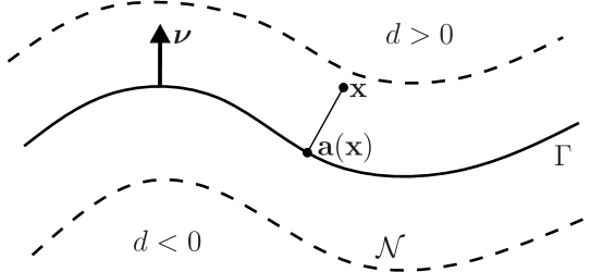
where H ˚ 1 ( Γ ) = { v ∈ H 1 ( Γ ) : ∫ Γ v 𝑑 A = 0 } superscript ˚ 𝐻 1 Γ conditional-set 𝑣 superscript 𝐻 1 Γ subscript Γ 𝑣 differential-d 𝐴 0 \mathaccent 23{H}^{1}(\Gamma)=\{v\in H^{1}(\Gamma):\,\int_{\Gamma}v\,dA=0\} ∇ Γ subscript bold-∇ Γ \operatorname{\boldsymbol{\nabla}_{\Gamma}} [MR3486164 ] , and (1 6 ∇ Γ v subscript bold-∇ Γ 𝑣 \operatorname{\boldsymbol{\nabla}_{\Gamma}}v Γ h subscript Γ ℎ \Gamma_{h} Γ Γ \Gamma Γ h subscript Γ ℎ \Gamma_{h} C 0 superscript 𝐶 0 C^{0} 𝒯 h subscript 𝒯 ℎ \mathcal{T}_{h} ∪ T ∈ 𝒯 h T = Γ h subscript 𝑇 subscript 𝒯 ℎ 𝑇 subscript Γ ℎ \cup_{T\in\mathcal{T}_{h}}T=\Gamma_{h} Γ Γ \Gamma h T = diam ( T ) subscript ℎ 𝑇 diam 𝑇 h_{T}=\operatorname{diam}(T) h = max { h T : T ∈ 𝒯 h } ℎ : subscript ℎ 𝑇 𝑇 subscript 𝒯 ℎ h=\max\{h_{T}:\,T\in\mathcal{T}_{h}\} T ∈ 𝒯 h 𝑇 subscript 𝒯 ℎ T\in\mathcal{T}_{h} 𝒩 T subscript 𝒩 𝑇 \mathcal{N}_{T} T 𝑇 T 𝒙 ∈ 𝒩 T 𝒙 subscript 𝒩 𝑇 {\boldsymbol{x}}\in\mathcal{N}_{T} 𝒂 ( 𝒙 ) ∈ Γ 𝒂 𝒙 Γ {\boldsymbol{a}}({\boldsymbol{x}})\in\Gamma 1
(2) 𝒙 = 𝒂 ( 𝒙 ) + d ( 𝒙 ) 𝝂 ( 𝒙 ) , 𝒙 𝒂 𝒙 𝑑 𝒙 𝝂 𝒙 {\boldsymbol{x}}={\boldsymbol{a}}({\boldsymbol{x}})+d({\boldsymbol{x}}){\boldsymbol{\nu}}({\boldsymbol{x}}),
d ( 𝒙 ) 𝑑 𝒙 d({\boldsymbol{x}}) signed distance function from 𝒙 𝒙 {\boldsymbol{x}} Γ Γ \Gamma 𝝂 ( 𝒂 ( 𝒙 ) ) 𝝂 𝒂 𝒙 {\boldsymbol{\nu}}({\boldsymbol{a}}({\boldsymbol{x}})) Γ Γ \Gamma 𝒂 ( 𝒙 ) 𝒂 𝒙 {\boldsymbol{a}}({\boldsymbol{x}}) 𝝂 ( 𝒂 ( 𝒙 ) ) = ( ∇ d ( 𝒙 ) ) t 𝝂 𝒂 𝒙 superscript bold-∇ 𝑑 𝒙 𝑡 {\boldsymbol{\nu}}({\boldsymbol{a}}({\boldsymbol{x}}))=(\operatorname{\boldsymbol{\operatorname{\nabla}}}d({\boldsymbol{x}}))^{t} 𝝂 ( 𝒙 ) = 𝝂 ( 𝒂 ( 𝒙 ) ) 𝝂 𝒙 𝝂 𝒂 𝒙 {\boldsymbol{\nu}}({\boldsymbol{x}})={\boldsymbol{\nu}}({\boldsymbol{a}}({\boldsymbol{x}})) 𝒙 ∈ 𝒩 T 𝒙 subscript 𝒩 𝑇 {\boldsymbol{x}}\in\mathcal{N}_{T} local tubular neighborhoods, we avoid unnecessary restrictions on the mesh size.
Here we would like to explain some notational conventions that we use. From now on, the gradient of a scalar function will be a row vector. The normal vector 𝝂 𝝂 {\boldsymbol{\nu}} 𝝂 h subscript 𝝂 ℎ {\boldsymbol{\nu}}_{h}
Figure 1. Diagram of closest point map (2 Γ Γ \Gamma 𝒩 𝒩 \mathcal{N} d 𝑑 d Γ Γ \Gamma d 𝑑 d Γ Γ \Gamma
We can now define, for every T ∈ 𝒯 h 𝑇 subscript 𝒯 ℎ T\in\mathcal{T}_{h} T ℓ = { 𝒂 ( 𝒙 ) : 𝒙 ∈ T } superscript 𝑇 ℓ conditional-set 𝒂 𝒙 𝒙 𝑇 T^{\ell}=\{{\boldsymbol{a}}({\boldsymbol{x}}):\,{\boldsymbol{x}}\in T\} Γ = ∪ T ∈ 𝒯 h T ℓ Γ subscript 𝑇 subscript 𝒯 ℎ superscript 𝑇 ℓ \Gamma=\cup_{T\in\mathcal{T}_{h}}T^{\ell} H ( 𝒂 ) = ∇ Γ 𝝂 ( 𝒂 ) 𝐻 𝒂 subscript bold-∇ Γ 𝝂 𝒂 H({\boldsymbol{a}})=\operatorname{\boldsymbol{\nabla}_{\Gamma}}{\boldsymbol{\nu}}({\boldsymbol{a}}) [MR0394451 ] . Since ∇ Γ 𝝂 = ∇ 𝝂 subscript bold-∇ Γ 𝝂 ∇ 𝝂 \operatorname{\boldsymbol{\nabla}_{\Gamma}}{\boldsymbol{\nu}}=\operatorname{\operatorname{\nabla}}{\boldsymbol{\nu}} H ( 𝒂 ( 𝒙 ) ) = ∇ 2 d ( 𝒙 ) 𝐻 𝒂 𝒙 superscript ∇ 2 𝑑 𝒙 H({\boldsymbol{a}}({\boldsymbol{x}}))=\operatorname{\operatorname{\nabla}}^{2}d({\boldsymbol{x}}) H ( 𝒙 ) = H ( 𝒂 ( 𝒙 ) ) 𝐻 𝒙 𝐻 𝒂 𝒙 H({\boldsymbol{x}})=H({\boldsymbol{a}}({\boldsymbol{x}})) 𝒙 ∈ 𝒩 T 𝒙 subscript 𝒩 𝑇 {\boldsymbol{x}}\in\mathcal{N}_{T}
At the estimates that follow in this paper we denote by C 𝐶 C h T subscript ℎ 𝑇 h_{T} u 𝑢 u f 𝑓 f Γ Γ \Gamma T ∈ 𝒯 h 𝑇 subscript 𝒯 ℎ T\in\mathcal{T}_{h}
Given T ∈ 𝒯 h 𝑇 subscript 𝒯 ℎ T\in\mathcal{T}_{h}
(3) κ T = ‖ H ‖ L ∞ ( T ) := max i j ‖ H i j ‖ L ∞ ( T ) , subscript 𝜅 𝑇 subscript norm 𝐻 superscript 𝐿 𝑇 assign subscript 𝑖 𝑗 subscript norm subscript 𝐻 𝑖 𝑗 superscript 𝐿 𝑇 \kappa_{T}=\|H\|_{L^{\infty}(T)}:=\max_{ij}\|H_{ij}\|_{L^{\infty}(T)},
and 𝝂 h ∈ ℝ 3 subscript 𝝂 ℎ superscript ℝ 3 {\boldsymbol{\nu}}_{h}\in\mathbb{R}^{3} T 𝑇 T 𝝂 h ⋅ 𝝂 > 0 ⋅ subscript 𝝂 ℎ 𝝂 0 {\boldsymbol{\nu}}_{h}\cdot{\boldsymbol{\nu}}>0 H 𝐻 H κ T subscript 𝜅 𝑇 \kappa_{T} L ∞ superscript 𝐿 L^{\infty} H 𝐻 H max { | k 1 | L ∞ ( T ) , | k 2 | L ∞ ( T ) } subscript subscript 𝑘 1 superscript 𝐿 𝑇 subscript subscript 𝑘 2 superscript 𝐿 𝑇 \max\{|k_{1}|_{L^{\infty}(T)},|k_{2}|_{L^{\infty}(T)}\} k i subscript 𝑘 𝑖 k_{i}
Assumption : Throughout the paper we will assume
(4) h T 2 κ T 2 ≤ c 1 < 1 for all T ∈ 𝒯 h , formulae-sequence superscript subscript ℎ 𝑇 2 superscript subscript 𝜅 𝑇 2 subscript 𝑐 1 1 for all 𝑇 subscript 𝒯 ℎ h_{T}^{2}\kappa_{T}^{2}\leq c_{1}<1\quad\text{for all }T\in\mathcal{T}_{h},
where c 1 subscript 𝑐 1 c_{1}
It is easy to see that
(5) ‖ d ‖ L ∞ ( T ) ≤ C h T 2 κ T , subscript norm 𝑑 superscript 𝐿 𝑇 𝐶 superscript subscript ℎ 𝑇 2 subscript 𝜅 𝑇 \displaystyle\|d\|_{L^{\infty}(T)}\leq Ch_{T}^{2}\kappa_{T},
(6) ‖ 𝝂 − 𝝂 h ‖ L ∞ ( T ) ≤ C h T κ T . subscript norm 𝝂 subscript 𝝂 ℎ superscript 𝐿 𝑇 𝐶 subscript ℎ 𝑇 subscript 𝜅 𝑇 \displaystyle\|{\boldsymbol{\nu}}-{\boldsymbol{\nu}}_{h}\|_{L^{\infty}(T)}\leq Ch_{T}\kappa_{T}.
To show (5 T ⊂ ℝ 2 × { 0 } 𝑇 superscript ℝ 2 0 T\subset\mathbb{R}^{2}\times\{0\} ν 3 subscript 𝜈 3 \nu_{3} ν 3 , h > 0 subscript 𝜈 3 ℎ
0 \nu_{3,h}>0 I h d subscript 𝐼 ℎ 𝑑 I_{h}d d 𝑑 d T 𝑇 T d 𝑑 d I h d ≡ 0 subscript 𝐼 ℎ 𝑑 0 I_{h}d\equiv 0 [MR2050138 ] we have
(7) ‖ d ‖ L ∞ ( T ) + h T ‖ ∂ d / ∂ x i ‖ L ∞ ( T ) = ‖ d − I h d ‖ L ∞ ( T ) + h T ‖ ∂ ( d − I h d ) / ∂ x i ‖ L ∞ ( T ) ≤ C h T 2 ‖ ∇ 2 d ‖ L ∞ ( T ) , subscript norm 𝑑 superscript 𝐿 𝑇 subscript ℎ 𝑇 subscript norm 𝑑 subscript 𝑥 𝑖 superscript 𝐿 𝑇 subscript norm 𝑑 subscript 𝐼 ℎ 𝑑 superscript 𝐿 𝑇 subscript ℎ 𝑇 subscript norm 𝑑 subscript 𝐼 ℎ 𝑑 subscript 𝑥 𝑖 superscript 𝐿 𝑇 𝐶 superscript subscript ℎ 𝑇 2 subscript norm superscript ∇ 2 𝑑 superscript 𝐿 𝑇 \|d\|_{L^{\infty}(T)}+h_{T}\|\partial d/\partial x_{i}\|_{L^{\infty}(T)}=\|d-I_{h}d\|_{L^{\infty}(T)}+h_{T}\|\partial(d-I_{h}d)/\partial x_{i}\|_{L^{\infty}(T)}\leq Ch_{T}^{2}\|\operatorname{\operatorname{\nabla}}^{2}d\|_{L^{\infty}(T)},
for i = 1 , 2 𝑖 1 2
i=1,2 6 𝝂 h t = ( 0 , 0 , 1 ) subscript superscript 𝝂 𝑡 ℎ 0 0 1 {\boldsymbol{\nu}}^{t}_{h}=(0,0,1) ‖ ν i ‖ L ∞ ( T ) = ‖ ∂ d / ∂ x i ‖ L ∞ ( T ) subscript norm subscript 𝜈 𝑖 superscript 𝐿 𝑇 subscript norm 𝑑 subscript 𝑥 𝑖 superscript 𝐿 𝑇 \|\nu_{i}\|_{L^{\infty}(T)}=\|\partial d/\partial x_{i}\|_{L^{\infty}(T)} 𝝂 𝝂 {\boldsymbol{\nu}} 7 3
‖ ν 3 − 1 ‖ L ∞ ( T ) ≤ ‖ ( ν 3 − 1 ) ( ν 3 + 1 ) ‖ L ∞ ( T ) = ‖ ν 3 2 − 1 ‖ L ∞ ( T ) ≤ ‖ ν 1 ‖ L ∞ ( T ) 2 + ‖ ν 2 ‖ L ∞ ( T ) 2 ≤ C h T 2 κ T 2 ≤ C h T κ T . subscript delimited-∥∥ subscript 𝜈 3 1 superscript 𝐿 𝑇 subscript delimited-∥∥ subscript 𝜈 3 1 subscript 𝜈 3 1 superscript 𝐿 𝑇 subscript delimited-∥∥ superscript subscript 𝜈 3 2 1 superscript 𝐿 𝑇 superscript subscript delimited-∥∥ subscript 𝜈 1 superscript 𝐿 𝑇 2 superscript subscript delimited-∥∥ subscript 𝜈 2 superscript 𝐿 𝑇 2 𝐶 superscript subscript ℎ 𝑇 2 superscript subscript 𝜅 𝑇 2 𝐶 subscript ℎ 𝑇 subscript 𝜅 𝑇 \|\nu_{3}-1\|_{L^{\infty}(T)}\leq\|(\nu_{3}-1)(\nu_{3}+1)\|_{L^{\infty}(T)}=\|\nu_{3}^{2}-1\|_{L^{\infty}(T)}\leq\|\nu_{1}\|_{L^{\infty}(T)}^{2}+\|\nu_{2}\|_{L^{\infty}(T)}^{2}\\
\leq Ch_{T}^{2}\kappa_{T}^{2}\leq Ch_{T}\kappa_{T}.
Here we used (4
From (5 3
(8) ‖ d H ‖ L ∞ ( T ) ≤ C h T 2 κ T 2 . subscript norm 𝑑 𝐻 superscript 𝐿 𝑇 𝐶 superscript subscript ℎ 𝑇 2 superscript subscript 𝜅 𝑇 2 \|dH\|_{L^{\infty}(T)}\leq Ch_{T}^{2}\kappa_{T}^{2}.
Therefore, making c 1 subscript 𝑐 1 c_{1} 4 d ( 𝒙 ) H ( 𝒙 ) 𝑑 𝒙 𝐻 𝒙 d({\boldsymbol{x}})H({\boldsymbol{x}}) 1 / 2 1 2 1/2 𝒙 ∈ Γ h 𝒙 subscript Γ ℎ {\boldsymbol{x}}\in\Gamma_{h}
(9) ‖ ( I − d H ) − 1 ‖ L ∞ ( T ) ≤ C . subscript norm superscript 𝐼 𝑑 𝐻 1 superscript 𝐿 𝑇 𝐶 \|(I-dH)^{-1}\|_{L^{\infty}(T)}\leq C.
We define tangential projections onto Γ Γ \Gamma Γ h subscript Γ ℎ \Gamma_{h} P = I − 𝝂 ⊗ 𝝂 𝑃 𝐼 tensor-product 𝝂 𝝂 P=I-{\boldsymbol{\nu}}\otimes{\boldsymbol{\nu}} P h = I − 𝝂 h ⊗ 𝝂 h subscript 𝑃 ℎ 𝐼 tensor-product subscript 𝝂 ℎ subscript 𝝂 ℎ P_{h}=I-{\boldsymbol{\nu}}_{h}\otimes{\boldsymbol{\nu}}_{h} 𝒒 ⊗ 𝒓 = 𝒒 𝒓 t tensor-product 𝒒 𝒓 𝒒 superscript 𝒓 𝑡 \boldsymbol{q}\otimes\boldsymbol{r}=\boldsymbol{q}\boldsymbol{r}^{t} 𝒒 𝒒 \boldsymbol{q} 𝒓 𝒓 \boldsymbol{r} Γ Γ \Gamma Γ h subscript Γ ℎ \Gamma_{h}
(10) ∇ Γ v = ( ∇ v ) P , ∇ Γ h v = ( ∇ v ) P h . formulae-sequence subscript bold-∇ Γ 𝑣 ∇ 𝑣 𝑃 subscript bold-∇ subscript Γ h 𝑣 ∇ 𝑣 subscript 𝑃 ℎ \operatorname{\boldsymbol{\nabla}_{\Gamma}}v=(\operatorname{\operatorname{\nabla}}v)P,\qquad\operatorname{\boldsymbol{\operatorname{\nabla}}_{\Gamma_{h}}}v=(\operatorname{\operatorname{\nabla}}v)P_{h}.
By using that 𝝂 ⋅ 𝝂 = 1 ⋅ 𝝂 𝝂 1 {\boldsymbol{\nu}}\cdot{\boldsymbol{\nu}}=1
(11) 0 = 1 2 ∇ ( 𝝂 ⋅ 𝝂 ) = ( ∇ 𝝂 ) 𝝂 = H ( 𝒙 ) 𝝂 ( 𝒙 ) for all 𝒙 ∈ T , 0 1 2 ∇ ⋅ 𝝂 𝝂 ∇ 𝝂 𝝂 𝐻 𝒙 𝝂 𝒙 for all 𝒙 𝑇 0=\frac{1}{2}\operatorname{\operatorname{\nabla}}({\boldsymbol{\nu}}\cdot{\boldsymbol{\nu}})=(\operatorname{\operatorname{\nabla}}{\boldsymbol{\nu}}){\boldsymbol{\nu}}=H({\boldsymbol{x}}){\boldsymbol{\nu}}({\boldsymbol{x}})\text{ for all }{\boldsymbol{x}}\in T,
Hence, we, of course, have
(12) P H = H = H P , 𝑃 𝐻 𝐻 𝐻 𝑃 PH=H=HP,
which we use repeatedly. Also, we can show that
(13) P ( I − d H ) − 1 𝝂 = 0 . 𝑃 superscript 𝐼 𝑑 𝐻 1 𝝂 0 P(I-dH)^{-1}{\boldsymbol{\nu}}=0.
Indeed, 𝝂 = ( I − d H ) 𝝂 𝝂 𝐼 𝑑 𝐻 𝝂 {\boldsymbol{\nu}}=(I-dH){\boldsymbol{\nu}} 11 P ( I − d H ) − 1 𝝂 = P ( I − d H ) − 1 ( I − d H ) 𝝂 = P 𝝂 = 0 𝑃 superscript 𝐼 𝑑 𝐻 1 𝝂 𝑃 superscript 𝐼 𝑑 𝐻 1 𝐼 𝑑 𝐻 𝝂 𝑃 𝝂 0 P(I-dH)^{-1}{\boldsymbol{\nu}}=P(I-dH)^{-1}(I-dH){\boldsymbol{\nu}}=P{\boldsymbol{\nu}}=0
2.1. Local parametrization
Let T ^ = { ( θ 1 , θ 2 ) : 0 ≤ θ 1 , θ 2 ≤ 1 , 0 ≤ θ 1 + θ 2 ≤ 1 } ^ 𝑇 conditional-set subscript 𝜃 1 subscript 𝜃 2 formulae-sequence 0 subscript 𝜃 1 formulae-sequence subscript 𝜃 2 1 0 subscript 𝜃 1 subscript 𝜃 2 1 \hat{T}=\{(\theta_{1},\theta_{2}):\,0\leq\theta_{1},\theta_{2}\leq 1,0\leq\theta_{1}+\theta_{2}\leq 1\} T ∈ 𝒯 h 𝑇 subscript 𝒯 ℎ T\in\mathcal{T}_{h} 𝒙 0 subscript 𝒙 0 {\boldsymbol{x}}_{0} 𝒙 1 subscript 𝒙 1 {\boldsymbol{x}}_{1} 𝒙 2 subscript 𝒙 2 {\boldsymbol{x}}_{2} ℝ 3 superscript ℝ 3 \mathbb{R}^{3} T 𝑇 T T = { 𝒙 0 + θ 1 𝒙 1 + θ 2 𝒙 2 : 0 ≤ θ 1 , θ 2 ≤ 1 , 0 ≤ θ 1 + θ 2 ≤ 1 } 𝑇 conditional-set subscript 𝒙 0 subscript 𝜃 1 subscript 𝒙 1 subscript 𝜃 2 subscript 𝒙 2 formulae-sequence 0 subscript 𝜃 1 formulae-sequence subscript 𝜃 2 1 0 subscript 𝜃 1 subscript 𝜃 2 1 T=\{{\boldsymbol{x}}_{0}+\theta_{1}{\boldsymbol{x}}_{1}+\theta_{2}{\boldsymbol{x}}_{2}:\,0\leq\theta_{1},\theta_{2}\leq 1,0\leq\theta_{1}+\theta_{2}\leq 1\} 𝑿 : T ^ → T : 𝑿 → ^ 𝑇 𝑇 {\boldsymbol{X}}:\hat{T}\rightarrow T 𝑿 ( θ 1 , θ 2 ) = 𝒙 0 + θ 1 𝒙 1 + θ 2 𝒙 2 𝑿 subscript 𝜃 1 subscript 𝜃 2 subscript 𝒙 0 subscript 𝜃 1 subscript 𝒙 1 subscript 𝜃 2 subscript 𝒙 2 {\boldsymbol{X}}(\theta_{1},\theta_{2})={\boldsymbol{x}}_{0}+\theta_{1}{\boldsymbol{x}}_{1}+\theta_{2}{\boldsymbol{x}}_{2} 𝒀 : T ^ → T ℓ : 𝒀 → ^ 𝑇 superscript 𝑇 ℓ {\boldsymbol{Y}}:\hat{T}\rightarrow T^{\ell} 𝒀 ( θ 1 , θ 2 ) = 𝒂 ( 𝑿 ( θ 1 , θ 2 ) ) 𝒀 subscript 𝜃 1 subscript 𝜃 2 𝒂 𝑿 subscript 𝜃 1 subscript 𝜃 2 {\boldsymbol{Y}}(\theta_{1},\theta_{2})={\boldsymbol{a}}({\boldsymbol{X}}(\theta_{1},\theta_{2})) ∇ 𝑿 = [ 𝒙 1 , 𝒙 2 ] ∇ 𝑿 subscript 𝒙 1 subscript 𝒙 2 \operatorname{\operatorname{\nabla}}{\boldsymbol{X}}=[{\boldsymbol{x}}_{1},{\boldsymbol{x}}_{2}] ( ∇ 𝑿 ) t 𝝂 h = 0 superscript ∇ 𝑿 𝑡 subscript 𝝂 ℎ 0 (\operatorname{\operatorname{\nabla}}{\boldsymbol{X}})^{t}{\boldsymbol{\nu}}_{h}=0 𝒂 𝒂 {\boldsymbol{a}}
∇ 𝒂 ( 𝒙 ) = P ( 𝒙 ) − d ( 𝒙 ) H ( 𝒙 ) , ∇ 𝒂 𝒙 𝑃 𝒙 𝑑 𝒙 𝐻 𝒙 \operatorname{\operatorname{\nabla}}{\boldsymbol{a}}({\boldsymbol{x}})=P({\boldsymbol{x}})-d({\boldsymbol{x}})H({\boldsymbol{x}}),
and, hence
(14) ∇ 𝒀 = ( P − d H ) ∇ X . ∇ 𝒀 𝑃 𝑑 𝐻 ∇ 𝑋 \operatorname{\operatorname{\nabla}}{\boldsymbol{Y}}=(P-dH)\operatorname{\operatorname{\nabla}}X.
Therefore, using that P 𝑃 P H 𝐻 H 11 ( ∇ 𝒀 ) t 𝝂 = 0 superscript ∇ 𝒀 𝑡 𝝂 0 (\operatorname{\operatorname{\nabla}}{\boldsymbol{Y}})^{t}{\boldsymbol{\nu}}=0
(15) ( ∇ 𝑿 ) t 𝝂 h = 0 , ( ∇ 𝒀 ) t 𝝂 = 0 . formulae-sequence superscript ∇ 𝑿 𝑡 subscript 𝝂 ℎ 0 superscript ∇ 𝒀 𝑡 𝝂 0 (\operatorname{\operatorname{\nabla}}{\boldsymbol{X}})^{t}{\boldsymbol{\nu}}_{h}=0,\qquad(\nabla{\boldsymbol{Y}})^{t}{\boldsymbol{\nu}}=0.
Given a function η ∈ L 1 ( T ℓ ) 𝜂 superscript 𝐿 1 superscript 𝑇 ℓ \eta\in L^{1}(T^{\ell}) η ℓ ∈ L 1 ( T ) subscript 𝜂 ℓ superscript 𝐿 1 𝑇 \eta_{\ell}\in L^{1}(T)
η ℓ ( 𝒙 ) = η ( 𝒂 ( 𝒙 ) ) , subscript 𝜂 ℓ 𝒙 𝜂 𝒂 𝒙 \eta_{\ell}({\boldsymbol{x}})=\eta({\boldsymbol{a}}({\boldsymbol{x}})),
and for η ∈ L 1 ( T ) 𝜂 superscript 𝐿 1 𝑇 \eta\in L^{1}(T) η ℓ ∈ L 1 ( T ℓ ) superscript 𝜂 ℓ superscript 𝐿 1 superscript 𝑇 ℓ \eta^{\ell}\in L^{1}(T^{\ell})
(16) η ℓ ( 𝒂 ( 𝒙 ) ) = η ( 𝒙 ) , superscript 𝜂 ℓ 𝒂 𝒙 𝜂 𝒙 \eta^{\ell}({\boldsymbol{a}}({\boldsymbol{x}}))=\eta({\boldsymbol{x}}),
and associate η ^ : T ^ → ℝ : ^ 𝜂 → ^ 𝑇 ℝ \hat{\eta}:\hat{T}\rightarrow\mathbb{R}
η ^ ( θ 1 , θ 2 ) = η ( 𝑿 ( θ 1 , θ 2 ) ) = η ℓ ( 𝒀 ( θ 1 , θ 2 ) ) . ^ 𝜂 subscript 𝜃 1 subscript 𝜃 2 𝜂 𝑿 subscript 𝜃 1 subscript 𝜃 2 superscript 𝜂 ℓ 𝒀 subscript 𝜃 1 subscript 𝜃 2 \hat{\eta}(\theta_{1},\theta_{2})=\eta({\boldsymbol{X}}(\theta_{1},\theta_{2}))=\eta^{\ell}({\boldsymbol{Y}}(\theta_{1},\theta_{2})).
Note that ( η ℓ ) ℓ = η superscript subscript 𝜂 ℓ ℓ 𝜂 (\eta_{\ell})^{\ell}=\eta η ∈ L 1 ( T ℓ ) 𝜂 superscript 𝐿 1 superscript 𝑇 ℓ \eta\in L^{1}(T^{\ell}) ( η ℓ ) ℓ = η subscript superscript 𝜂 ℓ ℓ 𝜂 (\eta^{\ell})_{\ell}=\eta η ∈ L 1 ( T ) 𝜂 superscript 𝐿 1 𝑇 \eta\in L^{1}(T)
Consider also the metric tensors
G 𝑿 ( θ 1 , θ 2 ) = ( ∇ 𝑿 ( θ 1 , θ 2 ) ) t ∇ 𝑿 ( θ 1 , θ 2 ) , G 𝒀 ( θ 1 , θ 2 ) = ( ∇ 𝒀 ( θ 1 , θ 2 ) ) t ∇ 𝒀 ( θ 1 , θ 2 ) . formulae-sequence subscript 𝐺 𝑿 subscript 𝜃 1 subscript 𝜃 2 superscript ∇ 𝑿 subscript 𝜃 1 subscript 𝜃 2 𝑡 ∇ 𝑿 subscript 𝜃 1 subscript 𝜃 2 subscript 𝐺 𝒀 subscript 𝜃 1 subscript 𝜃 2 superscript ∇ 𝒀 subscript 𝜃 1 subscript 𝜃 2 𝑡 ∇ 𝒀 subscript 𝜃 1 subscript 𝜃 2 G_{{\boldsymbol{X}}}(\theta_{1},\theta_{2})=\bigl{(}\operatorname{\operatorname{\nabla}}{\boldsymbol{X}}(\theta_{1},\theta_{2})\bigr{)}^{t}\operatorname{\operatorname{\nabla}}{\boldsymbol{X}}(\theta_{1},\theta_{2}),\qquad G_{{\boldsymbol{Y}}}(\theta_{1},\theta_{2})=\bigl{(}\operatorname{\operatorname{\nabla}}{\boldsymbol{Y}}(\theta_{1},\theta_{2})\bigr{)}^{t}\operatorname{\operatorname{\nabla}}{\boldsymbol{Y}}(\theta_{1},\theta_{2}).
From the definition of tangential derivative it is possible to show [MR3486164 ] *Section 4.2.1 (see also (2.2) in [MR3038698 ] ) that for a function η : Γ h → ℝ : 𝜂 → subscript Γ ℎ ℝ \eta:\Gamma_{h}\to\mathbb{R}
∇ Γ h η ( 𝑿 ) = ∇ η ^ G 𝑿 − 1 ∇ 𝑿 t , ∇ Γ η ℓ ( 𝒀 ) = ∇ η ^ G 𝒀 − 1 ∇ 𝒀 t , formulae-sequence subscript bold-∇ subscript Γ h 𝜂 𝑿 bold-∇ ^ 𝜂 superscript subscript 𝐺 𝑿 1 ∇ superscript 𝑿 𝑡 subscript bold-∇ Γ superscript 𝜂 ℓ 𝒀 bold-∇ ^ 𝜂 superscript subscript 𝐺 𝒀 1 ∇ superscript 𝒀 𝑡 \operatorname{\boldsymbol{\operatorname{\nabla}}_{\Gamma_{h}}}\eta({\boldsymbol{X}})=\operatorname{\boldsymbol{\operatorname{\nabla}}}\hat{\eta}G_{\boldsymbol{X}}^{-1}\operatorname{\operatorname{\nabla}}{\boldsymbol{X}}^{t},\qquad\operatorname{\boldsymbol{\nabla}_{\Gamma}}\eta^{\ell}({\boldsymbol{Y}})=\operatorname{\boldsymbol{\operatorname{\nabla}}}\hat{\eta}G_{\boldsymbol{Y}}^{-1}\operatorname{\operatorname{\nabla}}{\boldsymbol{Y}}^{t},
and multiplying by ∇ 𝑿 ∇ 𝑿 \operatorname{\operatorname{\nabla}}{\boldsymbol{X}} ∇ 𝒀 ∇ 𝒀 \operatorname{\operatorname{\nabla}}{\boldsymbol{Y}}
(17) ∇ η ^ = ∇ Γ h η ( 𝑿 ) ∇ 𝑿 , ∇ η ^ = ∇ Γ η ℓ ( 𝒀 ) ∇ 𝒀 . formulae-sequence bold-∇ ^ 𝜂 subscript bold-∇ subscript Γ h 𝜂 𝑿 ∇ 𝑿 bold-∇ ^ 𝜂 subscript bold-∇ Γ superscript 𝜂 ℓ 𝒀 ∇ 𝒀 \operatorname{\boldsymbol{\operatorname{\nabla}}}\hat{\eta}=\operatorname{\boldsymbol{\operatorname{\nabla}}_{\Gamma_{h}}}\eta({\boldsymbol{X}})\operatorname{\operatorname{\nabla}}{\boldsymbol{X}},\qquad\operatorname{\boldsymbol{\operatorname{\nabla}}}\hat{\eta}=\operatorname{\boldsymbol{\nabla}_{\Gamma}}\eta^{\ell}({\boldsymbol{Y}})\operatorname{\operatorname{\nabla}}{\boldsymbol{Y}}.
Hence,
(18) ∇ Γ h η ( 𝑿 ) = ∇ Γ η ℓ ( 𝒀 ) ∇ 𝒀 G 𝑿 − 1 ∇ 𝑿 t , subscript bold-∇ subscript Γ h 𝜂 𝑿 subscript bold-∇ Γ superscript 𝜂 ℓ 𝒀 ∇ 𝒀 superscript subscript 𝐺 𝑿 1 ∇ superscript 𝑿 𝑡 \displaystyle\operatorname{\boldsymbol{\operatorname{\nabla}}_{\Gamma_{h}}}\eta({\boldsymbol{X}})=\operatorname{\boldsymbol{\nabla}_{\Gamma}}\eta^{\ell}({\boldsymbol{Y}})\operatorname{\operatorname{\nabla}}{\boldsymbol{Y}}G_{\boldsymbol{X}}^{-1}\operatorname{\operatorname{\nabla}}{\boldsymbol{X}}^{t},
(19) ∇ Γ η ℓ ( 𝒀 ) = ∇ Γ h η ( 𝑿 ) ∇ 𝑿 G 𝒀 − 1 ∇ 𝒀 t . subscript bold-∇ Γ superscript 𝜂 ℓ 𝒀 subscript bold-∇ subscript Γ h 𝜂 𝑿 ∇ 𝑿 superscript subscript 𝐺 𝒀 1 ∇ superscript 𝒀 𝑡 \displaystyle\operatorname{\boldsymbol{\nabla}_{\Gamma}}\eta^{\ell}({\boldsymbol{Y}})=\operatorname{\boldsymbol{\operatorname{\nabla}}_{\Gamma_{h}}}\eta({\boldsymbol{X}})\operatorname{\operatorname{\nabla}}{\boldsymbol{X}}G_{\boldsymbol{Y}}^{-1}\operatorname{\operatorname{\nabla}}{\boldsymbol{Y}}^{t}.
Note that we can also write
(20) P = ∇ 𝒀 G 𝒀 − 1 ∇ 𝒀 t , P h = ∇ 𝑿 G 𝑿 − 1 ∇ 𝑿 t . formulae-sequence 𝑃 ∇ 𝒀 superscript subscript 𝐺 𝒀 1 ∇ superscript 𝒀 𝑡 subscript 𝑃 ℎ ∇ 𝑿 superscript subscript 𝐺 𝑿 1 ∇ superscript 𝑿 𝑡 P=\operatorname{\operatorname{\nabla}}{\boldsymbol{Y}}G_{\boldsymbol{Y}}^{-1}\operatorname{\operatorname{\nabla}}{\boldsymbol{Y}}^{t},\qquad P_{h}=\operatorname{\operatorname{\nabla}}{\boldsymbol{X}}G_{\boldsymbol{X}}^{-1}\operatorname{\operatorname{\nabla}}{\boldsymbol{X}}^{t}.
To see that this is the case, note first from (15 ∇ 𝒀 G 𝒀 − 1 ∇ 𝒀 t 𝝂 = 0 ∇ 𝒀 superscript subscript 𝐺 𝒀 1 ∇ superscript 𝒀 𝑡 𝝂 0 \operatorname{\operatorname{\nabla}}{\boldsymbol{Y}}G_{\boldsymbol{Y}}^{-1}\operatorname{\operatorname{\nabla}}{\boldsymbol{Y}}^{t}{\boldsymbol{\nu}}=0 ϵ > 0 italic-ϵ 0 \epsilon>0 𝒔 : ( − ϵ , ϵ ) → T ^ : 𝒔 → italic-ϵ italic-ϵ ^ 𝑇 {\boldsymbol{s}}:(-\epsilon,\epsilon)\to\hat{T} 𝜶 ( t ) = 𝒀 ( 𝒔 ( t ) ) 𝜶 𝑡 𝒀 𝒔 𝑡 {\boldsymbol{\alpha}}(t)={\boldsymbol{Y}}({\boldsymbol{s}}(t))
∇ 𝒀 G 𝒀 − 1 ∇ 𝒀 t 𝜶 ′ = ∇ 𝒀 G 𝒀 − 1 ∇ 𝒀 t ∇ 𝒀 𝒔 ′ = 𝜶 ′ = P 𝜶 ′ , ∇ 𝒀 superscript subscript 𝐺 𝒀 1 ∇ superscript 𝒀 𝑡 superscript 𝜶 ′ ∇ 𝒀 superscript subscript 𝐺 𝒀 1 ∇ superscript 𝒀 𝑡 ∇ 𝒀 superscript 𝒔 ′ superscript 𝜶 ′ 𝑃 superscript 𝜶 ′ \operatorname{\operatorname{\nabla}}{\boldsymbol{Y}}G_{\boldsymbol{Y}}^{-1}\operatorname{\operatorname{\nabla}}{\boldsymbol{Y}}^{t}{\boldsymbol{\alpha}}^{\prime}=\operatorname{\operatorname{\nabla}}{\boldsymbol{Y}}G_{\boldsymbol{Y}}^{-1}\operatorname{\operatorname{\nabla}}{\boldsymbol{Y}}^{t}\operatorname{\operatorname{\nabla}}{\boldsymbol{Y}}{\boldsymbol{s}}^{\prime}={\boldsymbol{\alpha}}^{\prime}=P{\boldsymbol{\alpha}}^{\prime},
since 𝜶 ′ superscript 𝜶 ′ {\boldsymbol{\alpha}}^{\prime} Γ Γ \Gamma P h subscript 𝑃 ℎ P_{h}
The following identities have appeared in the literature under different forms; see for example [MR2485433 , MR2285862 ] . Again, we give a proof for completeness and to show the independence of C 𝐶 C Γ Γ \Gamma
Lemma 1 .
Let η : Γ h → ℝ : 𝜂 → subscript Γ ℎ ℝ \eta:\Gamma_{h}\to\mathbb{R} η ℓ superscript 𝜂 ℓ \eta^{\ell} 16
(21) ∇ Γ h η = ( ∇ Γ η ℓ ∘ 𝒂 ) Q on Γ h , subscript bold-∇ subscript Γ h 𝜂 subscript bold-∇ Γ superscript 𝜂 ℓ 𝒂 𝑄 on subscript Γ ℎ
\operatorname{\boldsymbol{\operatorname{\nabla}}_{\Gamma_{h}}}\eta=(\operatorname{\boldsymbol{\nabla}_{\Gamma}}\eta^{\ell}\circ{\boldsymbol{a}})\,Q\quad\text{on }\Gamma_{h},
where Q = ( I − d H ) P h 𝑄 𝐼 𝑑 𝐻 subscript 𝑃 ℎ Q=(I-dH)P_{h}
(22) ∇ Γ η ℓ ∘ 𝒂 = ( ∇ Γ h η ) R on Γ h , subscript bold-∇ Γ superscript 𝜂 ℓ 𝒂 subscript bold-∇ subscript Γ h 𝜂 𝑅 on subscript Γ ℎ
\operatorname{\boldsymbol{\nabla}_{\Gamma}}\eta^{\ell}\circ{\boldsymbol{a}}=(\operatorname{\boldsymbol{\operatorname{\nabla}}_{\Gamma_{h}}}\eta)R\quad\text{on }\Gamma_{h},
where R = [ I − ( 𝛎 h − 𝛎 ) ⊗ ( 𝛎 − 𝛎 h ) 𝛎 h ⋅ 𝛎 ] ( I − d H ) − 1 P 𝑅 delimited-[] 𝐼 tensor-product subscript 𝛎 ℎ 𝛎 𝛎 subscript 𝛎 ℎ ⋅ subscript 𝛎 ℎ 𝛎 superscript 𝐼 𝑑 𝐻 1 𝑃 R=\bigl{[}I-\frac{({\boldsymbol{\nu}}_{h}-{\boldsymbol{\nu}})\otimes({\boldsymbol{\nu}}-{\boldsymbol{\nu}}_{h})}{{\boldsymbol{\nu}}_{h}\cdot{\boldsymbol{\nu}}}\bigr{]}(I-dH)^{-1}P C 𝐶 C
(23) ‖ Q ‖ L ∞ ( T ) + ‖ R ‖ L ∞ ( T ) ≤ C . subscript norm 𝑄 superscript 𝐿 𝑇 subscript norm 𝑅 superscript 𝐿 𝑇 𝐶 \|Q\|_{L^{\infty}(T)}+\|R\|_{L^{\infty}(T)}\leq C.
Proof.
Using (18 14
∇ Γ h η ( 𝑿 ) = ∇ Γ η ℓ ( 𝒀 ) [ I − d ( 𝑿 ) H ( 𝑿 ) ] ∇ 𝑿 G 𝑿 − 1 ∇ 𝑿 t subscript bold-∇ subscript Γ h 𝜂 𝑿 subscript bold-∇ Γ superscript 𝜂 ℓ 𝒀 delimited-[] 𝐼 𝑑 𝑿 𝐻 𝑿 ∇ 𝑿 superscript subscript 𝐺 𝑿 1 ∇ superscript 𝑿 𝑡 \operatorname{\boldsymbol{\operatorname{\nabla}}_{\Gamma_{h}}}\eta({\boldsymbol{X}})=\operatorname{\boldsymbol{\nabla}_{\Gamma}}\eta^{\ell}({\boldsymbol{Y}})[I-d({\boldsymbol{X}})H({\boldsymbol{X}})]\operatorname{\operatorname{\nabla}}{\boldsymbol{X}}G_{\boldsymbol{X}}^{-1}\operatorname{\operatorname{\nabla}}{\boldsymbol{X}}^{t}
where we used that ∇ Γ η ℓ 𝝂 ⊗ 𝝂 = 0 subscript bold-∇ Γ tensor-product superscript 𝜂 ℓ 𝝂 𝝂 0 \operatorname{\boldsymbol{\nabla}_{\Gamma}}\eta^{\ell}{\boldsymbol{\nu}}\otimes{\boldsymbol{\nu}}=0 21 20
To prove (22 14 12 ∇ 𝒀 = P [ I − d ( 𝑿 ) H ( 𝑿 ) ] ∇ 𝑿 ∇ 𝒀 𝑃 delimited-[] 𝐼 𝑑 𝑿 𝐻 𝑿 ∇ 𝑿 \operatorname{\operatorname{\nabla}}{\boldsymbol{Y}}=P[I-d({\boldsymbol{X}})H({\boldsymbol{X}})]\operatorname{\operatorname{\nabla}}{\boldsymbol{X}}
(24) ( ∇ 𝒀 ) t = ( ∇ 𝑿 ) t [ I − d ( 𝑿 ) H ( 𝑿 ) ] P . superscript ∇ 𝒀 𝑡 superscript ∇ 𝑿 𝑡 delimited-[] 𝐼 𝑑 𝑿 𝐻 𝑿 𝑃 (\operatorname{\operatorname{\nabla}}{\boldsymbol{Y}})^{t}=(\operatorname{\operatorname{\nabla}}{\boldsymbol{X}})^{t}[I-d({\boldsymbol{X}})H({\boldsymbol{X}})]P.
Using (12
( I − d H ) P ( I − d H ) − 1 ( I − 𝝂 h ⊗ 𝝂 𝝂 h ⋅ 𝝂 ) = P ( I − d H ) ( I − d H ) − 1 ( I − 𝝂 h ⊗ 𝝂 𝝂 h ⋅ 𝝂 ) = P ( I − 𝝂 h ⊗ 𝝂 𝝂 h ⋅ 𝝂 ) . 𝐼 𝑑 𝐻 𝑃 superscript 𝐼 𝑑 𝐻 1 𝐼 tensor-product subscript 𝝂 ℎ 𝝂 ⋅ subscript 𝝂 ℎ 𝝂 𝑃 𝐼 𝑑 𝐻 superscript 𝐼 𝑑 𝐻 1 𝐼 tensor-product subscript 𝝂 ℎ 𝝂 ⋅ subscript 𝝂 ℎ 𝝂 𝑃 𝐼 tensor-product subscript 𝝂 ℎ 𝝂 ⋅ subscript 𝝂 ℎ 𝝂 (I-dH)P(I-dH)^{-1}\biggl{(}I-\frac{{\boldsymbol{\nu}}_{h}\otimes{\boldsymbol{\nu}}}{{\boldsymbol{\nu}}_{h}\cdot{\boldsymbol{\nu}}}\biggr{)}=P(I-dH)(I-dH)^{-1}\biggl{(}I-\frac{{\boldsymbol{\nu}}_{h}\otimes{\boldsymbol{\nu}}}{{\boldsymbol{\nu}}_{h}\cdot{\boldsymbol{\nu}}}\biggr{)}=P\biggl{(}I-\frac{{\boldsymbol{\nu}}_{h}\otimes{\boldsymbol{\nu}}}{{\boldsymbol{\nu}}_{h}\cdot{\boldsymbol{\nu}}}\biggr{)}.
However,
P ( I − 𝝂 h ⊗ 𝝂 𝝂 h ⋅ 𝝂 ) = I − 𝝂 ⊗ 𝝂 − 𝝂 h ⊗ 𝝂 𝝂 h ⋅ 𝝂 + ( 𝝂 ⊗ 𝝂 ) 𝝂 h ⊗ 𝝂 𝝂 h ⋅ 𝝂 = I − 𝝂 h ⊗ 𝝂 𝝂 h ⋅ 𝝂 . 𝑃 𝐼 tensor-product subscript 𝝂 ℎ 𝝂 ⋅ subscript 𝝂 ℎ 𝝂 𝐼 tensor-product 𝝂 𝝂 tensor-product subscript 𝝂 ℎ 𝝂 ⋅ subscript 𝝂 ℎ 𝝂 tensor-product tensor-product 𝝂 𝝂 subscript 𝝂 ℎ 𝝂 ⋅ subscript 𝝂 ℎ 𝝂 𝐼 tensor-product subscript 𝝂 ℎ 𝝂 ⋅ subscript 𝝂 ℎ 𝝂 P\biggl{(}I-\frac{{\boldsymbol{\nu}}_{h}\otimes{\boldsymbol{\nu}}}{{\boldsymbol{\nu}}_{h}\cdot{\boldsymbol{\nu}}}\biggr{)}=I-{\boldsymbol{\nu}}\otimes{\boldsymbol{\nu}}-\frac{{\boldsymbol{\nu}}_{h}\otimes{\boldsymbol{\nu}}}{{\boldsymbol{\nu}}_{h}\cdot{\boldsymbol{\nu}}}+\frac{({\boldsymbol{\nu}}\otimes{\boldsymbol{\nu}}){\boldsymbol{\nu}}_{h}\otimes{\boldsymbol{\nu}}}{{\boldsymbol{\nu}}_{h}\cdot{\boldsymbol{\nu}}}=I-\frac{{\boldsymbol{\nu}}_{h}\otimes{\boldsymbol{\nu}}}{{\boldsymbol{\nu}}_{h}\cdot{\boldsymbol{\nu}}}.
This gives
(25) ( I − d H ) P ( I − d H ) − 1 ( I − 𝝂 h ⊗ 𝝂 𝝂 h ⋅ 𝝂 ) = I − 𝝂 h ⊗ 𝝂 𝝂 h ⋅ 𝝂 𝐼 𝑑 𝐻 𝑃 superscript 𝐼 𝑑 𝐻 1 𝐼 tensor-product subscript 𝝂 ℎ 𝝂 ⋅ subscript 𝝂 ℎ 𝝂 𝐼 tensor-product subscript 𝝂 ℎ 𝝂 ⋅ subscript 𝝂 ℎ 𝝂 (I-dH)P(I-dH)^{-1}\biggl{(}I-\frac{{\boldsymbol{\nu}}_{h}\otimes{\boldsymbol{\nu}}}{{\boldsymbol{\nu}}_{h}\cdot{\boldsymbol{\nu}}}\biggr{)}=I-\frac{{\boldsymbol{\nu}}_{h}\otimes{\boldsymbol{\nu}}}{{\boldsymbol{\nu}}_{h}\cdot{\boldsymbol{\nu}}}
So, from (25 24 15
( ∇ 𝒀 ) t ( I − d H ) − 1 ( I − 𝝂 h ⊗ 𝝂 𝝂 h ⋅ 𝝂 ) = ( ∇ 𝑿 ) t ( I − 𝝂 h ⊗ 𝝂 𝝂 h ⋅ 𝝂 ) = ( ∇ 𝑿 ) t . superscript ∇ 𝒀 𝑡 superscript 𝐼 𝑑 𝐻 1 𝐼 tensor-product subscript 𝝂 ℎ 𝝂 ⋅ subscript 𝝂 ℎ 𝝂 superscript ∇ 𝑿 𝑡 𝐼 tensor-product subscript 𝝂 ℎ 𝝂 ⋅ subscript 𝝂 ℎ 𝝂 superscript ∇ 𝑿 𝑡 (\operatorname{\operatorname{\nabla}}{\boldsymbol{Y}})^{t}(I-dH)^{-1}\biggl{(}I-\frac{{\boldsymbol{\nu}}_{h}\otimes{\boldsymbol{\nu}}}{{\boldsymbol{\nu}}_{h}\cdot{\boldsymbol{\nu}}}\biggr{)}=(\operatorname{\operatorname{\nabla}}{\boldsymbol{X}})^{t}\biggl{(}I-\frac{{\boldsymbol{\nu}}_{h}\otimes{\boldsymbol{\nu}}}{{\boldsymbol{\nu}}_{h}\cdot{\boldsymbol{\nu}}}\biggr{)}=(\operatorname{\operatorname{\nabla}}{\boldsymbol{X}})^{t}.
Thus, using (19
∇ Γ η ℓ ( 𝒀 ) = subscript bold-∇ Γ superscript 𝜂 ℓ 𝒀 absent \displaystyle\operatorname{\boldsymbol{\nabla}_{\Gamma}}\eta^{\ell}({\boldsymbol{Y}})= ∇ Γ h η ( 𝑿 ) ( I − 𝝂 ⊗ 𝝂 h 𝝂 h ⋅ 𝝂 ) ( I − d H ) − 1 ∇ 𝒀 G 𝒀 − 1 ∇ 𝒀 t subscript bold-∇ subscript Γ h 𝜂 𝑿 𝐼 tensor-product 𝝂 subscript 𝝂 ℎ ⋅ subscript 𝝂 ℎ 𝝂 superscript 𝐼 𝑑 𝐻 1 ∇ 𝒀 superscript subscript 𝐺 𝒀 1 ∇ superscript 𝒀 𝑡 \displaystyle\operatorname{\boldsymbol{\operatorname{\nabla}}_{\Gamma_{h}}}\eta({\boldsymbol{X}})\biggl{(}I-\frac{{\boldsymbol{\nu}}\otimes{\boldsymbol{\nu}}_{h}}{{\boldsymbol{\nu}}_{h}\cdot{\boldsymbol{\nu}}}\biggr{)}(I-dH)^{-1}\operatorname{\operatorname{\nabla}}{\boldsymbol{Y}}G_{\boldsymbol{Y}}^{-1}\operatorname{\operatorname{\nabla}}{\boldsymbol{Y}}^{t}
= \displaystyle= ∇ Γ h η ( 𝑿 ) ( I − 𝝂 ⊗ 𝝂 h 𝝂 h ⋅ 𝝂 ) ( I − d H ) − 1 P , subscript bold-∇ subscript Γ h 𝜂 𝑿 𝐼 tensor-product 𝝂 subscript 𝝂 ℎ ⋅ subscript 𝝂 ℎ 𝝂 superscript 𝐼 𝑑 𝐻 1 𝑃 \displaystyle\operatorname{\boldsymbol{\operatorname{\nabla}}_{\Gamma_{h}}}\eta({\boldsymbol{X}})\biggl{(}I-\frac{{\boldsymbol{\nu}}\otimes{\boldsymbol{\nu}}_{h}}{{\boldsymbol{\nu}}_{h}\cdot{\boldsymbol{\nu}}}\biggr{)}(I-dH)^{-1}P,
from (20 ( ∇ Γ h η ) 𝝂 h ⊗ 𝝂 h = 0 = ( ∇ Γ h η ) 𝝂 h ⊗ 𝝂 tensor-product subscript bold-∇ subscript Γ h 𝜂 subscript 𝝂 ℎ subscript 𝝂 ℎ 0 tensor-product subscript bold-∇ subscript Γ h 𝜂 subscript 𝝂 ℎ 𝝂 (\operatorname{\boldsymbol{\operatorname{\nabla}}_{\Gamma_{h}}}\eta)~{}{\boldsymbol{\nu}}_{h}\otimes{\boldsymbol{\nu}}_{h}=0=(\operatorname{\boldsymbol{\operatorname{\nabla}}_{\Gamma_{h}}}\eta)~{}{\boldsymbol{\nu}}_{h}\otimes{\boldsymbol{\nu}} P ( I − d H ) − 1 𝝂 ⊗ 𝝂 = 0 tensor-product 𝑃 superscript 𝐼 𝑑 𝐻 1 𝝂 𝝂 0 P(I-dH)^{-1}{\boldsymbol{\nu}}\otimes{\boldsymbol{\nu}}=0 13
∇ Γ η ℓ ( 𝒀 ) = ∇ Γ h η [ I − ( 𝝂 h − 𝝂 ) ⊗ ( 𝝂 − 𝝂 h ) 𝝂 h ⋅ 𝝂 ] ( I − d H ) − 1 P . subscript bold-∇ Γ superscript 𝜂 ℓ 𝒀 subscript bold-∇ subscript Γ h 𝜂 delimited-[] 𝐼 tensor-product subscript 𝝂 ℎ 𝝂 𝝂 subscript 𝝂 ℎ ⋅ subscript 𝝂 ℎ 𝝂 superscript 𝐼 𝑑 𝐻 1 𝑃 \operatorname{\boldsymbol{\nabla}_{\Gamma}}\eta^{\ell}({\boldsymbol{Y}})=\operatorname{\boldsymbol{\operatorname{\nabla}}_{\Gamma_{h}}}\eta\biggl{[}I-\frac{({\boldsymbol{\nu}}_{h}-{\boldsymbol{\nu}})\otimes({\boldsymbol{\nu}}-{\boldsymbol{\nu}}_{h})}{{\boldsymbol{\nu}}_{h}\cdot{\boldsymbol{\nu}}}\biggr{]}(I-dH)^{-1}P.
Here we used that ( 𝝂 h − 𝝂 ) ⊗ ( 𝝂 − 𝝂 h ) = − 𝝂 h ⊗ 𝝂 h − 𝝂 ⊗ 𝝂 + 𝝂 h ⊗ 𝝂 + 𝝂 ⊗ 𝝂 h tensor-product subscript 𝝂 ℎ 𝝂 𝝂 subscript 𝝂 ℎ tensor-product subscript 𝝂 ℎ subscript 𝝂 ℎ tensor-product 𝝂 𝝂 tensor-product subscript 𝝂 ℎ 𝝂 tensor-product 𝝂 subscript 𝝂 ℎ ({\boldsymbol{\nu}}_{h}-{\boldsymbol{\nu}})\otimes({\boldsymbol{\nu}}-{\boldsymbol{\nu}}_{h})=-{\boldsymbol{\nu}}_{h}\otimes{\boldsymbol{\nu}}_{h}-{\boldsymbol{\nu}}\otimes{\boldsymbol{\nu}}+{\boldsymbol{\nu}}_{h}\otimes{\boldsymbol{\nu}}+{\boldsymbol{\nu}}\otimes{\boldsymbol{\nu}}_{h} 22 23 6 8 9 4
Next, we write an integration identity.
Lemma 2 .
Let η ∈ L 1 ( T ) 𝜂 superscript 𝐿 1 𝑇 \eta\in L^{1}(T) d A 𝑑 𝐴 dA T ℓ superscript 𝑇 ℓ T^{\ell} d A h 𝑑 subscript 𝐴 ℎ dA_{h} T 𝑇 T
(26) ∫ T ℓ η ℓ 𝑑 A = ∫ T η δ T 𝑑 A h , subscript superscript 𝑇 ℓ superscript 𝜂 ℓ differential-d 𝐴 subscript 𝑇 𝜂 subscript 𝛿 𝑇 differential-d subscript 𝐴 ℎ \int_{T^{\ell}}\eta^{\ell}\,dA=\int_{T}\eta\delta_{T}\,dA_{h},
where
(27) δ T = det ( G 𝒀 G 𝑿 − 1 ) . subscript 𝛿 𝑇 subscript 𝐺 𝒀 superscript subscript 𝐺 𝑿 1 \delta_{T}=\sqrt{\det(G_{\boldsymbol{Y}}G_{\boldsymbol{X}}^{-1})}.
Proof.
The result follows from the change of variables formulas [MR0394451 ]
∫ T ℓ η ℓ 𝑑 A = ∫ T ^ η ^ det G 𝒀 𝑑 θ 1 𝑑 θ 2 , ∫ T ^ η ^ det G 𝑿 − 1 𝑑 θ 1 𝑑 θ 2 = ∫ T η 𝑑 A h . formulae-sequence subscript superscript 𝑇 ℓ superscript 𝜂 ℓ differential-d 𝐴 subscript ^ 𝑇 ^ 𝜂 subscript 𝐺 𝒀 differential-d subscript 𝜃 1 differential-d subscript 𝜃 2 subscript ^ 𝑇 ^ 𝜂 superscript subscript 𝐺 𝑿 1 differential-d subscript 𝜃 1 differential-d subscript 𝜃 2 subscript 𝑇 𝜂 differential-d subscript 𝐴 ℎ \int_{T^{\ell}}\eta^{\ell}\,dA=\int_{\hat{T}}\hat{\eta}\sqrt{\det G_{\boldsymbol{Y}}}\,d\theta_{1}\,d\theta_{2},\qquad\int_{\hat{T}}\hat{\eta}\sqrt{\det G_{\boldsymbol{X}}^{-1}}\,d\theta_{1}\,d\theta_{2}=\int_{T}\eta\,dA_{h}.
∎
Combining (26 21 22
(28) ∫ T ∇ Γ h η ⋅ ∇ Γ h ψ d A h = ∫ T ℓ ∇ Γ η ℓ Q ℓ ⋅ ∇ Γ ψ ℓ Q ℓ 1 δ T ℓ d A , subscript 𝑇 subscript bold-∇ subscript Γ h ⋅ 𝜂 subscript bold-∇ subscript Γ h 𝜓 𝑑 subscript 𝐴 ℎ subscript superscript 𝑇 ℓ subscript bold-∇ Γ ⋅ superscript 𝜂 ℓ superscript 𝑄 ℓ subscript bold-∇ Γ superscript 𝜓 ℓ superscript 𝑄 ℓ 1 superscript subscript 𝛿 𝑇 ℓ 𝑑 𝐴 \displaystyle\int_{T}\operatorname{\boldsymbol{\operatorname{\nabla}}_{\Gamma_{h}}}\eta\cdot\operatorname{\boldsymbol{\operatorname{\nabla}}_{\Gamma_{h}}}\psi\,dA_{h}=\int_{T^{\ell}}\operatorname{\boldsymbol{\nabla}_{\Gamma}}\eta^{\ell}Q^{\ell}\cdot\operatorname{\boldsymbol{\nabla}_{\Gamma}}\psi^{\ell}Q^{\ell}\frac{1}{\delta_{T}^{\ell}}\,dA,
(29) ∫ T ℓ ∇ Γ η ℓ ⋅ ∇ Γ ψ ℓ d A = ∫ T ∇ Γ h η R ⋅ ∇ Γ h ψ R δ T d A h . subscript superscript 𝑇 ℓ subscript bold-∇ Γ ⋅ superscript 𝜂 ℓ subscript bold-∇ Γ superscript 𝜓 ℓ 𝑑 𝐴 subscript 𝑇 subscript bold-∇ subscript Γ h ⋅ 𝜂 𝑅 subscript bold-∇ subscript Γ h 𝜓 𝑅 subscript 𝛿 𝑇 𝑑 subscript 𝐴 ℎ \displaystyle\int_{T^{\ell}}\operatorname{\boldsymbol{\nabla}_{\Gamma}}\eta^{\ell}\cdot\operatorname{\boldsymbol{\nabla}_{\Gamma}}\psi^{\ell}\,dA=\int_{T}\operatorname{\boldsymbol{\operatorname{\nabla}}_{\Gamma_{h}}}\eta R\cdot\operatorname{\boldsymbol{\operatorname{\nabla}}_{\Gamma_{h}}}\psi R\delta_{T}\,dA_{h}.
Next, we prove some bounds for δ T subscript 𝛿 𝑇 \delta_{T}
Lemma 3 .
Assuming that (4 δ T subscript 𝛿 𝑇 \delta_{T} 27
(30) ‖ δ T − 1 ‖ L ∞ ( T ) ≤ C h T 2 κ T 2 , subscript norm subscript 𝛿 𝑇 1 superscript 𝐿 𝑇 𝐶 superscript subscript ℎ 𝑇 2 superscript subscript 𝜅 𝑇 2 \displaystyle\|\delta_{T}-1\|_{L^{\infty}(T)}\leq Ch_{T}^{2}\kappa_{T}^{2},
(31) ‖ 1 δ T − 1 ‖ L ∞ ( T ) ≤ C h T 2 κ T 2 . subscript norm 1 subscript 𝛿 𝑇 1 superscript 𝐿 𝑇 𝐶 superscript subscript ℎ 𝑇 2 superscript subscript 𝜅 𝑇 2 \displaystyle\|\frac{1}{\delta_{T}}-1\|_{L^{\infty}(T)}\leq Ch_{T}^{2}\kappa_{T}^{2}.
Proof.
From (14 15
G 𝒀 = ∇ 𝑿 t ( I − d H − 𝝂 ⊗ 𝝂 ) ∇ 𝒀 = ∇ 𝑿 t ( I − d H ) ∇ 𝒀 = ∇ 𝑿 t ( I − d H ) 2 ∇ 𝑿 − ∇ 𝑿 t ( I − d H ) 𝝂 ⊗ 𝝂 ∇ 𝑿 . subscript 𝐺 𝒀 ∇ superscript 𝑿 𝑡 𝐼 𝑑 𝐻 tensor-product 𝝂 𝝂 ∇ 𝒀 ∇ superscript 𝑿 𝑡 𝐼 𝑑 𝐻 ∇ 𝒀 ∇ superscript 𝑿 𝑡 superscript 𝐼 𝑑 𝐻 2 ∇ 𝑿 tensor-product ∇ superscript 𝑿 𝑡 𝐼 𝑑 𝐻 𝝂 𝝂 ∇ 𝑿 G_{\boldsymbol{Y}}=\operatorname{\operatorname{\nabla}}{\boldsymbol{X}}^{t}(I-dH-{\boldsymbol{\nu}}\otimes{\boldsymbol{\nu}})\operatorname{\operatorname{\nabla}}{\boldsymbol{Y}}=\operatorname{\operatorname{\nabla}}{\boldsymbol{X}}^{t}(I-dH)\operatorname{\operatorname{\nabla}}{\boldsymbol{Y}}\\
=\operatorname{\operatorname{\nabla}}{\boldsymbol{X}}^{t}(I-dH)^{2}\operatorname{\operatorname{\nabla}}{\boldsymbol{X}}-\operatorname{\operatorname{\nabla}}{\boldsymbol{X}}^{t}(I-dH){\boldsymbol{\nu}}\otimes{\boldsymbol{\nu}}\operatorname{\operatorname{\nabla}}{\boldsymbol{X}}.
Using (11
( ∇ 𝑿 ) t ( I − d H ) 𝝂 ⊗ 𝝂 ∇ 𝑿 = ∇ 𝑿 t 𝝂 ⊗ 𝝂 ∇ 𝑿 . tensor-product superscript ∇ 𝑿 𝑡 𝐼 𝑑 𝐻 𝝂 𝝂 ∇ 𝑿 ∇ tensor-product superscript 𝑿 𝑡 𝝂 𝝂 ∇ 𝑿 (\operatorname{\operatorname{\nabla}}{\boldsymbol{X}})^{t}(I-dH){\boldsymbol{\nu}}\otimes{\boldsymbol{\nu}}\operatorname{\operatorname{\nabla}}{\boldsymbol{X}}=\operatorname{\operatorname{\nabla}}{\boldsymbol{X}}^{t}{\boldsymbol{\nu}}\otimes{\boldsymbol{\nu}}\operatorname{\operatorname{\nabla}}{\boldsymbol{X}}.
By (15
( ∇ 𝑿 ) t 𝝂 h ⊗ 𝝂 h ∇ 𝑿 = ( ∇ 𝑿 ) t 𝝂 h ⊗ 𝝂 ∇ 𝑿 = ( ∇ 𝑿 ) t 𝝂 ⊗ 𝝂 h ∇ 𝑿 = 0 . tensor-product superscript ∇ 𝑿 𝑡 subscript 𝝂 ℎ subscript 𝝂 ℎ ∇ 𝑿 tensor-product superscript ∇ 𝑿 𝑡 subscript 𝝂 ℎ 𝝂 ∇ 𝑿 tensor-product superscript ∇ 𝑿 𝑡 𝝂 subscript 𝝂 ℎ ∇ 𝑿 0 (\operatorname{\operatorname{\nabla}}{\boldsymbol{X}})^{t}{\boldsymbol{\nu}}_{h}\otimes{\boldsymbol{\nu}}_{h}\operatorname{\operatorname{\nabla}}{\boldsymbol{X}}=(\operatorname{\operatorname{\nabla}}{\boldsymbol{X}})^{t}{\boldsymbol{\nu}}_{h}\otimes{\boldsymbol{\nu}}\operatorname{\operatorname{\nabla}}{\boldsymbol{X}}=(\operatorname{\operatorname{\nabla}}{\boldsymbol{X}})^{t}{\boldsymbol{\nu}}\otimes{\boldsymbol{\nu}}_{h}\operatorname{\operatorname{\nabla}}{\boldsymbol{X}}=0.
Hence,
( ∇ 𝑿 ) t 𝝂 ⊗ 𝝂 ∇ 𝑿 = ( ∇ 𝑿 ) t ( 𝝂 − 𝝂 h ) ⊗ ( 𝝂 − 𝝂 h ) ∇ 𝑿 . tensor-product superscript ∇ 𝑿 𝑡 𝝂 𝝂 ∇ 𝑿 tensor-product superscript ∇ 𝑿 𝑡 𝝂 subscript 𝝂 ℎ 𝝂 subscript 𝝂 ℎ ∇ 𝑿 (\operatorname{\operatorname{\nabla}}{\boldsymbol{X}})^{t}{\boldsymbol{\nu}}\otimes{\boldsymbol{\nu}}\operatorname{\operatorname{\nabla}}{\boldsymbol{X}}=(\operatorname{\operatorname{\nabla}}{\boldsymbol{X}})^{t}({\boldsymbol{\nu}}-{\boldsymbol{\nu}}_{h})\otimes({\boldsymbol{\nu}}-{\boldsymbol{\nu}}_{h})\operatorname{\operatorname{\nabla}}{\boldsymbol{X}}.
Therefore, we get
G 𝒀 = ( ∇ 𝑿 ) t [ ( I − d H ) 2 − ( 𝝂 − 𝝂 h ) ⊗ ( 𝝂 − 𝝂 h ) ] ∇ 𝑿 , subscript 𝐺 𝒀 superscript ∇ 𝑿 𝑡 delimited-[] superscript 𝐼 𝑑 𝐻 2 tensor-product 𝝂 subscript 𝝂 ℎ 𝝂 subscript 𝝂 ℎ ∇ 𝑿 G_{\boldsymbol{Y}}=(\operatorname{\operatorname{\nabla}}{\boldsymbol{X}})^{t}[(I-dH)^{2}-({\boldsymbol{\nu}}-{\boldsymbol{\nu}}_{h})\otimes({\boldsymbol{\nu}}-{\boldsymbol{\nu}}_{h})]\operatorname{\operatorname{\nabla}}{\boldsymbol{X}},
or G 𝒀 = ( ∇ 𝑿 ) t ( I + B ) ∇ 𝑿 subscript 𝐺 𝒀 superscript ∇ 𝑿 𝑡 𝐼 𝐵 ∇ 𝑿 G_{\boldsymbol{Y}}=(\operatorname{\operatorname{\nabla}}{\boldsymbol{X}})^{t}(I+B)\operatorname{\operatorname{\nabla}}{\boldsymbol{X}} B = − 2 d H + d 2 H 2 − ( 𝝂 − 𝝂 h ) ⊗ ( 𝝂 − 𝝂 h ) 𝐵 2 𝑑 𝐻 superscript 𝑑 2 superscript 𝐻 2 tensor-product 𝝂 subscript 𝝂 ℎ 𝝂 subscript 𝝂 ℎ B=-2dH+d^{2}H^{2}-({\boldsymbol{\nu}}-{\boldsymbol{\nu}}_{h})\otimes({\boldsymbol{\nu}}-{\boldsymbol{\nu}}_{h})
G 𝒀 G 𝑿 − 1 = I + M where M = ∇ 𝑿 t B ∇ 𝑿 G 𝑿 − 1 . formulae-sequence subscript 𝐺 𝒀 superscript subscript 𝐺 𝑿 1 𝐼 𝑀 where 𝑀 ∇ superscript 𝑿 𝑡 𝐵 ∇ 𝑿 superscript subscript 𝐺 𝑿 1 G_{\boldsymbol{Y}}G_{\boldsymbol{X}}^{-1}=I+M\quad\text{where }M=\operatorname{\operatorname{\nabla}}{\boldsymbol{X}}^{t}B\operatorname{\operatorname{\nabla}}{\boldsymbol{X}}G_{\boldsymbol{X}}^{-1}.
It is clear that ‖ ∇ 𝑿 ‖ L ∞ ( T ) ≤ C h T subscript norm ∇ 𝑿 superscript 𝐿 𝑇 𝐶 subscript ℎ 𝑇 \|\operatorname{\operatorname{\nabla}}{\boldsymbol{X}}\|_{L^{\infty}(T)}\leq Ch_{T} ‖ G 𝑿 − 1 ‖ L ∞ ( T ) ≤ C h T − 2 subscript norm superscript subscript 𝐺 𝑿 1 superscript 𝐿 𝑇 𝐶 superscript subscript ℎ 𝑇 2 \|G_{\boldsymbol{X}}^{-1}\|_{L^{\infty}(T)}\leq Ch_{T}^{-2} 6 8 ‖ B ‖ L ∞ ( T ) ≤ C h T 2 κ T 2 subscript norm 𝐵 superscript 𝐿 𝑇 𝐶 superscript subscript ℎ 𝑇 2 superscript subscript 𝜅 𝑇 2 \|B\|_{L^{\infty}(T)}\leq Ch_{T}^{2}\kappa_{T}^{2} ‖ M ‖ L ∞ ( T ) ≤ C h T 2 κ T 2 subscript norm 𝑀 superscript 𝐿 𝑇 𝐶 superscript subscript ℎ 𝑇 2 superscript subscript 𝜅 𝑇 2 \|M\|_{L^{\infty}(T)}\leq Ch_{T}^{2}\kappa_{T}^{2} M 𝑀 M M = V Λ V − 1 𝑀 𝑉 Λ superscript 𝑉 1 M=V\Lambda V^{-1} Λ = diag ( λ 1 , λ 2 ) Λ diag subscript 𝜆 1 subscript 𝜆 2 \Lambda=\operatorname{diag}(\lambda_{1},\lambda_{2}) V 𝑉 V V 𝑉 V v i subscript 𝑣 𝑖 v_{i} λ i = v i t M v i subscript 𝜆 𝑖 superscript subscript 𝑣 𝑖 𝑡 𝑀 subscript 𝑣 𝑖 \lambda_{i}=v_{i}^{t}Mv_{i} ‖ λ i ‖ L ∞ ( T ) ≤ C h T 2 κ T 2 subscript norm subscript 𝜆 𝑖 superscript 𝐿 𝑇 𝐶 superscript subscript ℎ 𝑇 2 superscript subscript 𝜅 𝑇 2 \|\lambda_{i}\|_{L^{\infty}(T)}\leq Ch_{T}^{2}\kappa_{T}^{2} i = 1 , 2 𝑖 1 2
i=1,2
G 𝒀 G 𝑿 − 1 = I + V Λ V − 1 = V ( I + Λ ) V − 1 . subscript 𝐺 𝒀 superscript subscript 𝐺 𝑿 1 𝐼 𝑉 Λ superscript 𝑉 1 𝑉 𝐼 Λ superscript 𝑉 1 G_{\boldsymbol{Y}}G_{\boldsymbol{X}}^{-1}=I+V\Lambda V^{-1}=V(I+\Lambda)V^{-1}.
Therefore, we obtain
δ T 2 = det ( G 𝒀 G 𝑿 − 1 ) = det ( V ) det ( I + Λ ) det ( V − 1 ) = ( 1 + λ 1 ) ( 1 + λ 2 ) , superscript subscript 𝛿 𝑇 2 subscript 𝐺 𝒀 superscript subscript 𝐺 𝑿 1 𝑉 𝐼 Λ superscript 𝑉 1 1 subscript 𝜆 1 1 subscript 𝜆 2 \delta_{T}^{2}=\det(G_{\boldsymbol{Y}}G_{\boldsymbol{X}}^{-1})=\det(V)\det(I+\Lambda)\det(V^{-1})=(1+\lambda_{1})(1+\lambda_{2}),
which yields
‖ δ T 2 − 1 ‖ L ∞ ( T ) ≤ C h T 2 κ T 2 . subscript norm superscript subscript 𝛿 𝑇 2 1 superscript 𝐿 𝑇 𝐶 superscript subscript ℎ 𝑇 2 superscript subscript 𝜅 𝑇 2 \|\delta_{T}^{2}-1\|_{L^{\infty}(T)}\leq Ch_{T}^{2}\kappa_{T}^{2}.
Using that δ T − 1 = ( δ T 2 − 1 ) / ( δ T + 1 ) subscript 𝛿 𝑇 1 superscript subscript 𝛿 𝑇 2 1 subscript 𝛿 𝑇 1 \delta_{T}-1=(\delta_{T}^{2}-1)/(\delta_{T}+1) 30 31 ( δ T − 1 − 1 ) = δ T − 1 ( 1 − δ T ) superscript subscript 𝛿 𝑇 1 1 superscript subscript 𝛿 𝑇 1 1 subscript 𝛿 𝑇 (\delta_{T}^{-1}-1)=\delta_{T}^{-1}(1-\delta_{T})
We can now state the following result which follows from Lemmas 1 3 28 29
Lemma 4 .
Assuming the hypotheses of Lemmas 1 3
‖ ∇ Γ η ℓ ‖ L 2 ( T ℓ ) ≤ C ‖ ∇ Γ h η ‖ L 2 ( T ) ≤ C ‖ ∇ Γ η ℓ ‖ L 2 ( T ℓ ) . subscript norm subscript bold-∇ Γ superscript 𝜂 ℓ superscript 𝐿 2 superscript 𝑇 ℓ 𝐶 subscript norm subscript bold-∇ subscript Γ h 𝜂 superscript 𝐿 2 𝑇 𝐶 subscript norm subscript bold-∇ Γ superscript 𝜂 ℓ superscript 𝐿 2 superscript 𝑇 ℓ \|\operatorname{\boldsymbol{\nabla}_{\Gamma}}\eta^{\ell}\|_{L^{2}(T^{\ell})}\leq C\|\operatorname{\boldsymbol{\operatorname{\nabla}}_{\Gamma_{h}}}\eta\|_{L^{2}(T)}\leq C\|\operatorname{\boldsymbol{\nabla}_{\Gamma}}\eta^{\ell}\|_{L^{2}(T^{\ell})}.
In the following, we use the notation D ¯ i u = ( ∇ Γ u ) i subscript ¯ 𝐷 𝑖 𝑢 subscript subscript bold-∇ Γ 𝑢 𝑖 \underline{D}_{i}u=(\operatorname{\boldsymbol{\nabla}_{\Gamma}}u)_{i} ∇ Γ 2 u superscript subscript ∇ Γ 2 𝑢 \operatorname{\operatorname{\nabla_{\Gamma}^{2}}}u 3 × 3 3 3 3\times 3 D ¯ i D ¯ j u subscript ¯ 𝐷 𝑖 subscript ¯ 𝐷 𝑗 𝑢 \underline{D}_{i}\underline{D}_{j}u D ¯ i j u subscript ¯ 𝐷 𝑖 𝑗 𝑢 \underline{D}_{ij}u
Lemma 5 .
Assuming that (4
‖ ∇ Γ h 2 η ‖ L 2 ( T ) ≤ C ‖ ∇ Γ 2 η ℓ ‖ L 2 ( T ℓ ) + C ( h T κ T 2 + h T 2 κ T γ T ) ‖ ∇ Γ η ℓ ‖ L 2 ( T ℓ ) , subscript norm superscript subscript ∇ subscript Γ ℎ 2 𝜂 superscript 𝐿 2 𝑇 𝐶 subscript norm superscript subscript ∇ Γ 2 superscript 𝜂 ℓ superscript 𝐿 2 superscript 𝑇 ℓ 𝐶 subscript ℎ 𝑇 superscript subscript 𝜅 𝑇 2 superscript subscript ℎ 𝑇 2 subscript 𝜅 𝑇 subscript 𝛾 𝑇 subscript norm subscript bold-∇ Γ superscript 𝜂 ℓ superscript 𝐿 2 superscript 𝑇 ℓ \|\operatorname{\operatorname{\nabla}}_{\Gamma_{h}}^{2}\eta\|_{L^{2}(T)}\leq C\|\operatorname{\operatorname{\nabla_{\Gamma}^{2}}}\eta^{\ell}\|_{L^{2}(T^{\ell})}+C(h_{T}\kappa_{T}^{2}+h_{T}^{2}\kappa_{T}\gamma_{T})\|\operatorname{\boldsymbol{\nabla}_{\Gamma}}\eta^{\ell}\|_{L^{2}(T^{\ell})},
where γ T = max i j ‖ ∇ H i j ‖ L ∞ ( T ) subscript 𝛾 𝑇 subscript 𝑖 𝑗 subscript norm bold-∇ subscript 𝐻 𝑖 𝑗 superscript 𝐿 𝑇 \gamma_{T}=\max_{ij}\|\operatorname{\boldsymbol{\operatorname{\nabla}}}H_{ij}\|_{L^{\infty}(T)}
Proof.
Let 𝒘 = ∇ Γ h η 𝒘 subscript bold-∇ subscript Γ h 𝜂 {\boldsymbol{w}}=\operatorname{\boldsymbol{\operatorname{\nabla}}_{\Gamma_{h}}}\eta 21 𝒙 ∈ T 𝒙 𝑇 {\boldsymbol{x}}\in T
w i ( 𝒙 ) = ( P h ) i k ( I − d ( 𝒙 ) H ( 𝒙 ) ) k j D ¯ j η ℓ ( 𝒂 ( 𝒙 ) ) , subscript 𝑤 𝑖 𝒙 subscript subscript 𝑃 ℎ 𝑖 𝑘 subscript 𝐼 𝑑 𝒙 𝐻 𝒙 𝑘 𝑗 subscript ¯ 𝐷 𝑗 superscript 𝜂 ℓ 𝒂 𝒙 w_{i}({\boldsymbol{x}})=(P_{h})_{ik}\bigl{(}I-d({\boldsymbol{x}})H({\boldsymbol{x}})\bigr{)}_{kj}\underline{D}_{j}\eta^{\ell}({\boldsymbol{a}}({\boldsymbol{x}})),
where we use Einstein summation convention.
Using the product rule and the fact that P h subscript 𝑃 ℎ P_{h}
∇ Γ h w i ( 𝒙 ) = 𝑱 1 ( 𝒙 ) + 𝑱 2 ( 𝒙 ) + 𝑱 3 ( 𝒙 ) , subscript bold-∇ subscript Γ h subscript 𝑤 𝑖 𝒙 subscript 𝑱 1 𝒙 subscript 𝑱 2 𝒙 subscript 𝑱 3 𝒙 \operatorname{\boldsymbol{\operatorname{\nabla}}_{\Gamma_{h}}}w_{i}({\boldsymbol{x}})={\boldsymbol{J}}_{1}({\boldsymbol{x}})+{\boldsymbol{J}}_{2}({\boldsymbol{x}})+{\boldsymbol{J}}_{3}({\boldsymbol{x}}),
where
𝑱 1 = − ( P h ) i k H k j D ¯ j η ℓ ∘ 𝒂 ∇ Γ h d , 𝑱 2 = − ( P h ) i k d D ¯ j η ℓ ∘ 𝒂 ∇ Γ h H k j , 𝑱 3 = ( P h ) i k ( I − d H ) k j ∇ Γ h ( D ¯ j η ℓ ∘ 𝒂 ) . formulae-sequence subscript 𝑱 1 subscript subscript 𝑃 ℎ 𝑖 𝑘 subscript 𝐻 𝑘 𝑗 subscript ¯ 𝐷 𝑗 superscript 𝜂 ℓ 𝒂 subscript bold-∇ subscript Γ h 𝑑 formulae-sequence subscript 𝑱 2 subscript subscript 𝑃 ℎ 𝑖 𝑘 𝑑 subscript ¯ 𝐷 𝑗 superscript 𝜂 ℓ 𝒂 subscript bold-∇ subscript Γ h subscript 𝐻 𝑘 𝑗 subscript 𝑱 3 subscript subscript 𝑃 ℎ 𝑖 𝑘 subscript 𝐼 𝑑 𝐻 𝑘 𝑗 subscript bold-∇ subscript Γ h subscript ¯ 𝐷 𝑗 superscript 𝜂 ℓ 𝒂 \begin{split}{\boldsymbol{J}}_{1}&=-(P_{h})_{ik}H_{kj}\underline{D}_{j}\eta^{\ell}\circ{\boldsymbol{a}}\operatorname{\boldsymbol{\operatorname{\nabla}}_{\Gamma_{h}}}d,\\
{\boldsymbol{J}}_{2}&=-(P_{h})_{ik}d\underline{D}_{j}\eta^{\ell}\circ{\boldsymbol{a}}\operatorname{\boldsymbol{\operatorname{\nabla}}_{\Gamma_{h}}}H_{kj},\\
{\boldsymbol{J}}_{3}&=(P_{h})_{ik}(I-dH)_{kj}\operatorname{\boldsymbol{\operatorname{\nabla}}_{\Gamma_{h}}}(\underline{D}_{j}\eta^{\ell}\circ{\boldsymbol{a}}).\end{split}
We start with 𝑱 3 subscript 𝑱 3 {\boldsymbol{J}}_{3} 21
∇ Γ h ( D ¯ j η ℓ ∘ 𝒂 ) ( x ) = ∇ Γ D ¯ j η ℓ ( 𝒂 ( x ) ) Q subscript bold-∇ subscript Γ h subscript ¯ 𝐷 𝑗 superscript 𝜂 ℓ 𝒂 𝑥 subscript bold-∇ Γ subscript ¯ 𝐷 𝑗 superscript 𝜂 ℓ 𝒂 𝑥 𝑄 \operatorname{\boldsymbol{\operatorname{\nabla}}_{\Gamma_{h}}}(\underline{D}_{j}\eta^{\ell}\circ{\boldsymbol{a}})(x)=\operatorname{\boldsymbol{\nabla}_{\Gamma}}\underline{D}_{j}\eta^{\ell}({\boldsymbol{a}}(x))Q
Hence, using (23 26 30 4
‖ ∇ Γ h ( D ¯ j η ℓ ∘ 𝒂 ) ‖ L 2 ( T ) ≤ C ‖ ∇ Γ 2 η ℓ ‖ L 2 ( T ℓ ) . subscript norm subscript bold-∇ subscript Γ h subscript ¯ 𝐷 𝑗 superscript 𝜂 ℓ 𝒂 superscript 𝐿 2 𝑇 𝐶 subscript norm superscript subscript bold-∇ Γ 2 superscript 𝜂 ℓ superscript 𝐿 2 superscript 𝑇 ℓ \|\operatorname{\boldsymbol{\operatorname{\nabla}}_{\Gamma_{h}}}(\underline{D}_{j}\eta^{\ell}\circ{\boldsymbol{a}})\|_{L^{2}(T)}\leq C\|\operatorname{\boldsymbol{\nabla}_{\Gamma}}^{2}\eta^{\ell}\|_{L^{2}(T^{\ell})}.
If we combine this inequality with (8 4
‖ 𝑱 3 ‖ L 2 ( T ) ) ≤ C ‖ ∇ Γ 2 η ℓ ‖ L 2 ( T ℓ ) . \|{\boldsymbol{J}}_{3}\|_{L^{2}(T))}\leq C\|\operatorname{\boldsymbol{\nabla}_{\Gamma}}^{2}\eta^{\ell}\|_{L^{2}(T^{\ell})}.
Next, using (10 𝝂 h t P h = 0 superscript subscript 𝝂 ℎ 𝑡 subscript 𝑃 ℎ 0 {\boldsymbol{\nu}}_{h}^{t}P_{h}=0
∇ Γ h d = ( ∇ d ) P h = 𝝂 t P h = ( 𝝂 − 𝝂 h ) t P h . subscript bold-∇ subscript Γ h 𝑑 ∇ 𝑑 subscript 𝑃 ℎ superscript 𝝂 𝑡 subscript 𝑃 ℎ superscript 𝝂 subscript 𝝂 ℎ 𝑡 subscript 𝑃 ℎ \operatorname{\boldsymbol{\operatorname{\nabla}}_{\Gamma_{h}}}d=(\operatorname{\operatorname{\nabla}}d)P_{h}={\boldsymbol{\nu}}^{t}P_{h}=({\boldsymbol{\nu}}-{\boldsymbol{\nu}}_{h})^{t}P_{h}.
Hence, using (6 3 26 30 4
‖ 𝑱 1 ‖ L 2 ( T ) ≤ C h T κ T 2 ‖ ∇ Γ η ℓ ‖ L 2 ( T ℓ ) . subscript norm subscript 𝑱 1 superscript 𝐿 2 𝑇 𝐶 subscript ℎ 𝑇 superscript subscript 𝜅 𝑇 2 subscript norm subscript bold-∇ Γ superscript 𝜂 ℓ superscript 𝐿 2 superscript 𝑇 ℓ \|{\boldsymbol{J}}_{1}\|_{L^{2}(T)}\leq Ch_{T}\kappa_{T}^{2}\|\operatorname{\boldsymbol{\nabla}_{\Gamma}}\eta^{\ell}\|_{L^{2}(T^{\ell})}.
Similarly, (5 26 30 4
‖ 𝑱 2 ‖ L 2 ( T ) ≤ C h T 2 κ T γ T ‖ ∇ Γ η ℓ ‖ L 2 ( T ℓ ) . subscript norm subscript 𝑱 2 superscript 𝐿 2 𝑇 𝐶 superscript subscript ℎ 𝑇 2 subscript 𝜅 𝑇 subscript 𝛾 𝑇 subscript norm subscript bold-∇ Γ superscript 𝜂 ℓ superscript 𝐿 2 superscript 𝑇 ℓ \|{\boldsymbol{J}}_{2}\|_{L^{2}(T)}\leq Ch_{T}^{2}\kappa_{T}\gamma_{T}\|\operatorname{\boldsymbol{\nabla}_{\Gamma}}\eta^{\ell}\|_{L^{2}(T^{\ell})}.
Combining the above estimates gives the desired result.
∎
3. Finite Element Spaces and local approximations
We introduce the following finite dimensional approximation of (1
S h = { v h ∈ C 0 ( Γ h ) : ∫ Γ h v h 𝑑 A h = 0 , v h | T is linear for all T ∈ 𝒯 h } , S h ℓ = { v h ℓ : v h ∈ S h } . formulae-sequence subscript 𝑆 ℎ conditional-set subscript 𝑣 ℎ superscript 𝐶 0 subscript Γ ℎ formulae-sequence subscript subscript Γ ℎ subscript 𝑣 ℎ differential-d subscript 𝐴 ℎ 0 evaluated-at subscript 𝑣 ℎ 𝑇 is linear for all 𝑇 subscript 𝒯 ℎ superscript subscript 𝑆 ℎ ℓ conditional-set superscript subscript 𝑣 ℎ ℓ subscript 𝑣 ℎ subscript 𝑆 ℎ S_{h}=\{v_{h}\in C^{0}(\Gamma_{h}):\,\int_{\Gamma_{h}}v_{h}\,dA_{h}=0,\,v_{h}|_{T}\text{ is linear for all }T\in\mathcal{T}_{h}\},\qquad S_{h}^{\ell}=\{v_{h}^{\ell}:\,v_{h}\in S_{h}\}.
For f h ∈ L 2 ( Γ h ) subscript 𝑓 ℎ superscript 𝐿 2 subscript Γ ℎ f_{h}\in L^{2}(\Gamma_{h}) ∫ Γ h f h 𝑑 A h = 0 subscript subscript Γ ℎ subscript 𝑓 ℎ differential-d subscript 𝐴 ℎ 0 \int_{\Gamma_{h}}f_{h}\,dA_{h}=0 u h ∈ S h subscript 𝑢 ℎ subscript 𝑆 ℎ u_{h}\in S_{h}
(32) ∫ Γ h ∇ Γ h u h ⋅ ∇ Γ h v h d A h = ∫ Γ h f h v h 𝑑 A h for all v h ∈ S h . formulae-sequence subscript subscript Γ ℎ subscript bold-∇ subscript Γ h ⋅ subscript 𝑢 ℎ subscript bold-∇ subscript Γ h subscript 𝑣 ℎ 𝑑 subscript 𝐴 ℎ subscript subscript Γ ℎ subscript 𝑓 ℎ subscript 𝑣 ℎ differential-d subscript 𝐴 ℎ for all subscript 𝑣 ℎ subscript 𝑆 ℎ \int_{\Gamma_{h}}\operatorname{\boldsymbol{\operatorname{\nabla}}_{\Gamma_{h}}}u_{h}\cdot\operatorname{\boldsymbol{\operatorname{\nabla}}_{\Gamma_{h}}}v_{h}\,dA_{h}=\int_{\Gamma_{h}}f_{h}v_{h}\,dA_{h}\qquad\text{for all }v_{h}\in S_{h}.
Existence and uniqueness of the finite-dimensional problem (32 u h subscript 𝑢 ℎ u_{h} f h = 0 subscript 𝑓 ℎ 0 f_{h}=0 u h subscript 𝑢 ℎ u_{h} u h = 0 subscript 𝑢 ℎ 0 u_{h}=0
We will need a Poincaré’s inequality, as follows [MR3038698 ] .
Lemma 6 .
Assuming Γ ⊂ ℝ 3 Γ superscript ℝ 3 \Gamma\subset\mathbb{R}^{3} C 3 superscript 𝐶 3 C^{3} c p subscript 𝑐 𝑝 c_{p}
(33) ‖ ϕ ‖ L 2 ( Γ ) ≤ c p ‖ ∇ Γ ϕ ‖ L 2 ( Γ ) for all ϕ ∈ H ˚ 1 ( Γ ) . formulae-sequence subscript norm italic-ϕ superscript 𝐿 2 Γ subscript 𝑐 𝑝 subscript norm subscript bold-∇ Γ italic-ϕ superscript 𝐿 2 Γ for all italic-ϕ superscript ˚ 𝐻 1 Γ \|\phi\|_{L^{2}(\Gamma)}\leq c_{p}\|\operatorname{\boldsymbol{\nabla}_{\Gamma}}\phi\|_{L^{2}(\Gamma)}\qquad\text{ for all }\phi\in\mathaccent 23{H}^{1}(\Gamma).
Then we can state a simple energy estimate.
Lemma 7 .
Let u 𝑢 u 1
(34) ‖ ∇ Γ u ‖ L 2 ( Γ ) ≤ c p ‖ f ‖ L 2 ( Γ ) . subscript norm subscript bold-∇ Γ 𝑢 superscript 𝐿 2 Γ subscript 𝑐 𝑝 subscript norm 𝑓 superscript 𝐿 2 Γ \|\operatorname{\boldsymbol{\nabla}_{\Gamma}}u\|_{L^{2}(\Gamma)}\leq c_{p}\|f\|_{L^{2}(\Gamma)}.
Before proving an a-priori estimate for u h ℓ − u subscript superscript 𝑢 ℓ ℎ 𝑢 u^{\ell}_{h}-u Γ Γ \Gamma Γ h subscript Γ ℎ \Gamma_{h} δ T d A h = d A subscript 𝛿 𝑇 𝑑 subscript 𝐴 ℎ 𝑑 𝐴 \delta_{T}dA_{h}=dA T 𝑇 T T ℓ superscript 𝑇 ℓ T^{\ell}
δ h ( 𝒙 ) = δ T , if 𝒙 ∈ T . formulae-sequence subscript 𝛿 ℎ 𝒙 subscript 𝛿 𝑇 if 𝒙 𝑇 \delta_{h}({\boldsymbol{x}})=\delta_{T},\quad\text{if }{\boldsymbol{x}}\in T.
Lemma 8 .
Let v h subscript 𝑣 ℎ v_{h} z h subscript 𝑧 ℎ z_{h} S h subscript 𝑆 ℎ S_{h}
(35) | ∫ Γ h ∇ Γ h v h ⋅ ∇ Γ h z h d A h − ∫ Γ ∇ Γ v h ℓ ⋅ ∇ Γ z h ℓ d A | ≤ C Ψ h ‖ ∇ Γ v h ℓ ‖ L 2 ( Γ ) ‖ ∇ Γ z h ℓ ‖ L 2 ( Γ ) subscript subscript Γ ℎ subscript bold-∇ subscript Γ h ⋅ subscript 𝑣 ℎ subscript bold-∇ subscript Γ h subscript 𝑧 ℎ 𝑑 subscript 𝐴 ℎ subscript Γ subscript bold-∇ Γ ⋅ superscript subscript 𝑣 ℎ ℓ subscript bold-∇ Γ superscript subscript 𝑧 ℎ ℓ 𝑑 𝐴 𝐶 subscript Ψ ℎ subscript norm subscript bold-∇ Γ superscript subscript 𝑣 ℎ ℓ superscript 𝐿 2 Γ subscript norm subscript bold-∇ Γ superscript subscript 𝑧 ℎ ℓ superscript 𝐿 2 Γ \displaystyle|\int_{\Gamma_{h}}\operatorname{\boldsymbol{\operatorname{\nabla}}_{\Gamma_{h}}}v_{h}\cdot\operatorname{\boldsymbol{\operatorname{\nabla}}_{\Gamma_{h}}}z_{h}\,dA_{h}-\int_{\Gamma}\operatorname{\boldsymbol{\nabla}_{\Gamma}}v_{h}^{\ell}\cdot\operatorname{\boldsymbol{\nabla}_{\Gamma}}z_{h}^{\ell}\,dA|\leq C\Psi_{h}\|\operatorname{\boldsymbol{\nabla}_{\Gamma}}v_{h}^{\ell}\|_{L^{2}(\Gamma)}\|\operatorname{\boldsymbol{\nabla}_{\Gamma}}z_{h}^{\ell}\|_{L^{2}(\Gamma)}
(36) | ∫ Γ h v h z h 𝑑 A h − ∫ Γ v h ℓ z h ℓ 𝑑 A | ≤ C Ψ h ‖ v h ℓ ‖ L 2 ( Γ ) ‖ z h ℓ ‖ L 2 ( Γ ) , subscript subscript Γ ℎ subscript 𝑣 ℎ subscript 𝑧 ℎ differential-d subscript 𝐴 ℎ subscript Γ superscript subscript 𝑣 ℎ ℓ superscript subscript 𝑧 ℎ ℓ differential-d 𝐴 𝐶 subscript Ψ ℎ subscript norm superscript subscript 𝑣 ℎ ℓ superscript 𝐿 2 Γ subscript norm superscript subscript 𝑧 ℎ ℓ superscript 𝐿 2 Γ \displaystyle|\int_{\Gamma_{h}}v_{h}z_{h}\,dA_{h}-\int_{\Gamma}v_{h}^{\ell}z_{h}^{\ell}\,dA|\leq C\Psi_{h}\|v_{h}^{\ell}\|_{L^{2}(\Gamma)}\|z_{h}^{\ell}\|_{L^{2}(\Gamma)},
where Ψ h = max T ∈ 𝒯 h κ T 2 h T 2 subscript Ψ ℎ subscript 𝑇 subscript 𝒯 ℎ superscript subscript 𝜅 𝑇 2 superscript subscript ℎ 𝑇 2 \Psi_{h}=\max_{T\in\mathcal{T}_{h}}\kappa_{T}^{2}h_{T}^{2}
Proof.
Using (26
| ∫ Γ h v h z h 𝑑 A h − ∫ Γ v h ℓ z h ℓ 𝑑 A | = | ∫ Γ v h ℓ z h ℓ ( 1 δ h ℓ − 1 ) 𝑑 A | subscript subscript Γ ℎ subscript 𝑣 ℎ subscript 𝑧 ℎ differential-d subscript 𝐴 ℎ subscript Γ superscript subscript 𝑣 ℎ ℓ superscript subscript 𝑧 ℎ ℓ differential-d 𝐴 subscript Γ superscript subscript 𝑣 ℎ ℓ superscript subscript 𝑧 ℎ ℓ 1 superscript subscript 𝛿 ℎ ℓ 1 differential-d 𝐴 |\int_{\Gamma_{h}}v_{h}z_{h}\,dA_{h}-\int_{\Gamma}v_{h}^{\ell}z_{h}^{\ell}\,dA|=|\int_{\Gamma}v_{h}^{\ell}z_{h}^{\ell}\,(\frac{1}{\delta_{h}^{\ell}}-1)\,dA|
Hence, (36 31
To prove (35 28
∫ Γ h ∇ Γ h v h ⋅ ∇ Γ h z h d A h = ∫ Γ ( ∇ Γ v h ℓ Q ℓ ) ⋅ ( ∇ Γ z h ℓ Q ℓ ) 1 δ h ℓ 𝑑 A . subscript subscript Γ ℎ subscript bold-∇ subscript Γ h ⋅ subscript 𝑣 ℎ subscript bold-∇ subscript Γ h subscript 𝑧 ℎ 𝑑 subscript 𝐴 ℎ subscript Γ ⋅ subscript bold-∇ Γ superscript subscript 𝑣 ℎ ℓ superscript 𝑄 ℓ subscript bold-∇ Γ superscript subscript 𝑧 ℎ ℓ superscript 𝑄 ℓ 1 superscript subscript 𝛿 ℎ ℓ differential-d 𝐴 \int_{\Gamma_{h}}\operatorname{\boldsymbol{\operatorname{\nabla}}_{\Gamma_{h}}}v_{h}\cdot\operatorname{\boldsymbol{\operatorname{\nabla}}_{\Gamma_{h}}}z_{h}\,dA_{h}=\int_{\Gamma}(\operatorname{\boldsymbol{\nabla}_{\Gamma}}v_{h}^{\ell}Q^{\ell})\cdot(\operatorname{\boldsymbol{\nabla}_{\Gamma}}z_{h}^{\ell}Q^{\ell})\frac{1}{\delta_{h}^{\ell}}\,dA.
Using that ∇ Γ ( ⋅ ) P = ∇ Γ ( ⋅ ) subscript bold-∇ Γ ⋅ 𝑃 subscript bold-∇ Γ ⋅ \operatorname{\boldsymbol{\nabla}_{\Gamma}}(\cdot)P=\operatorname{\boldsymbol{\nabla}_{\Gamma}}(\cdot)
∫ Γ h ∇ Γ h v h ⋅ ∇ Γ h z h d A h = ∫ Γ ∇ Γ v h ℓ M ⋅ ∇ Γ z h ℓ d A , subscript subscript Γ ℎ subscript bold-∇ subscript Γ h ⋅ subscript 𝑣 ℎ subscript bold-∇ subscript Γ h subscript 𝑧 ℎ 𝑑 subscript 𝐴 ℎ subscript Γ subscript bold-∇ Γ ⋅ superscript subscript 𝑣 ℎ ℓ 𝑀 subscript bold-∇ Γ superscript subscript 𝑧 ℎ ℓ 𝑑 𝐴 \int_{\Gamma_{h}}\operatorname{\boldsymbol{\operatorname{\nabla}}_{\Gamma_{h}}}v_{h}\cdot\operatorname{\boldsymbol{\operatorname{\nabla}}_{\Gamma_{h}}}z_{h}\,dA_{h}=\int_{\Gamma}\operatorname{\boldsymbol{\nabla}_{\Gamma}}v_{h}^{\ell}M\cdot\operatorname{\boldsymbol{\nabla}_{\Gamma}}z_{h}^{\ell}\,dA,
where
M = 1 δ h ℓ ( P Q ℓ ) ( P Q ℓ ) t . 𝑀 1 superscript subscript 𝛿 ℎ ℓ 𝑃 superscript 𝑄 ℓ superscript 𝑃 superscript 𝑄 ℓ 𝑡 M=\frac{1}{\delta_{h}^{\ell}}(PQ^{\ell})(PQ^{\ell})^{t}.
On the other hand, again using that ∇ Γ ( ⋅ ) P = ∇ Γ ( ⋅ ) subscript bold-∇ Γ ⋅ 𝑃 subscript bold-∇ Γ ⋅ \operatorname{\boldsymbol{\nabla}_{\Gamma}}(\cdot)P=\operatorname{\boldsymbol{\nabla}_{\Gamma}}(\cdot)
∫ Γ ∇ Γ v h ℓ ⋅ ∇ Γ z h ℓ d A = ∫ Γ ∇ Γ v h ℓ P ⋅ ∇ Γ z h ℓ d A . subscript Γ subscript bold-∇ Γ ⋅ superscript subscript 𝑣 ℎ ℓ subscript bold-∇ Γ superscript subscript 𝑧 ℎ ℓ 𝑑 𝐴 subscript Γ subscript bold-∇ Γ ⋅ superscript subscript 𝑣 ℎ ℓ 𝑃 subscript bold-∇ Γ superscript subscript 𝑧 ℎ ℓ 𝑑 𝐴 \int_{\Gamma}\operatorname{\boldsymbol{\nabla}_{\Gamma}}v_{h}^{\ell}\cdot\operatorname{\boldsymbol{\nabla}_{\Gamma}}z_{h}^{\ell}\,dA=\int_{\Gamma}\operatorname{\boldsymbol{\nabla}_{\Gamma}}v_{h}^{\ell}P\cdot\operatorname{\boldsymbol{\nabla}_{\Gamma}}z_{h}^{\ell}\,dA.
Hence,
(37) | ∫ Γ h ∇ Γ h v h ⋅ ∇ Γ h z h d A h − ∫ Γ ∇ Γ v h ℓ ⋅ ∇ Γ z h ℓ d A | = | ∫ Γ ∇ Γ v h ℓ ( M − P ) ⋅ ∇ Γ z h ℓ d A | . subscript subscript Γ ℎ subscript bold-∇ subscript Γ h ⋅ subscript 𝑣 ℎ subscript bold-∇ subscript Γ h subscript 𝑧 ℎ 𝑑 subscript 𝐴 ℎ subscript Γ subscript bold-∇ Γ ⋅ superscript subscript 𝑣 ℎ ℓ subscript bold-∇ Γ superscript subscript 𝑧 ℎ ℓ 𝑑 𝐴 subscript Γ ⋅ subscript bold-∇ Γ superscript subscript 𝑣 ℎ ℓ 𝑀 𝑃 subscript bold-∇ Γ superscript subscript 𝑧 ℎ ℓ 𝑑 𝐴 |\int_{\Gamma_{h}}\operatorname{\boldsymbol{\operatorname{\nabla}}_{\Gamma_{h}}}v_{h}\cdot\operatorname{\boldsymbol{\operatorname{\nabla}}_{\Gamma_{h}}}z_{h}\,dA_{h}-\int_{\Gamma}\operatorname{\boldsymbol{\nabla}_{\Gamma}}v_{h}^{\ell}\cdot\operatorname{\boldsymbol{\nabla}_{\Gamma}}z_{h}^{\ell}\,dA|=|\int_{\Gamma}\operatorname{\boldsymbol{\nabla}_{\Gamma}}v_{h}^{\ell}(M-P)\cdot\operatorname{\boldsymbol{\nabla}_{\Gamma}}z_{h}^{\ell}\,dA|.
We now proceed to bound ( M − P ) 𝑀 𝑃 (M-P) 12 Γ h subscript Γ ℎ \Gamma_{h}
P Q ℓ ∘ 𝒂 = P Q = P ( I − d H ) P h = ( I − d H ) P P h . 𝑃 superscript 𝑄 ℓ 𝒂 𝑃 𝑄 𝑃 𝐼 𝑑 𝐻 subscript 𝑃 ℎ 𝐼 𝑑 𝐻 𝑃 subscript 𝑃 ℎ PQ^{\ell}\circ{\boldsymbol{a}}=PQ=P(I-dH)P_{h}=(I-dH)PP_{h}.
Hence, we get
M ∘ 𝒂 = 1 δ h ( I − d H ) S ( I − d H ) , 𝑀 𝒂 1 subscript 𝛿 ℎ 𝐼 𝑑 𝐻 𝑆 𝐼 𝑑 𝐻 M\circ{\boldsymbol{a}}=\frac{1}{\delta_{h}}(I-dH)S(I-dH),
where S = P P h P 𝑆 𝑃 subscript 𝑃 ℎ 𝑃 S=PP_{h}P
‖ M − P ‖ L ∞ ( T ℓ ) = subscript norm 𝑀 𝑃 superscript 𝐿 superscript 𝑇 ℓ absent \displaystyle\|M-P\|_{L^{\infty}(T^{\ell})}= ‖ δ h − 1 ( I − d H ) S ( I − d H ) − P ‖ L ∞ ( T ) subscript norm superscript subscript 𝛿 ℎ 1 𝐼 𝑑 𝐻 𝑆 𝐼 𝑑 𝐻 𝑃 superscript 𝐿 𝑇 \displaystyle\|\delta_{h}^{-1}(I-dH)S(I-dH)-P\|_{L^{\infty}(T)}
≤ \displaystyle\leq ‖ δ h − 1 ( I − d H ) S ( I − d H ) − S ‖ L ∞ ( T ) + ‖ S − P ‖ L ∞ ( T ) . subscript norm superscript subscript 𝛿 ℎ 1 𝐼 𝑑 𝐻 𝑆 𝐼 𝑑 𝐻 𝑆 superscript 𝐿 𝑇 subscript norm 𝑆 𝑃 superscript 𝐿 𝑇 \displaystyle\|\delta_{h}^{-1}(I-dH)S(I-dH)-S\|_{L^{\infty}(T)}+\|S-P\|_{L^{\infty}(T)}.
Now using (8 4 31 S 𝑆 S
‖ δ h − 1 ( I − d H ) S ( I − d H ) − S ‖ L ∞ ( T ) ≤ C h T 2 κ T 2 . subscript norm superscript subscript 𝛿 ℎ 1 𝐼 𝑑 𝐻 𝑆 𝐼 𝑑 𝐻 𝑆 superscript 𝐿 𝑇 𝐶 superscript subscript ℎ 𝑇 2 superscript subscript 𝜅 𝑇 2 \|\delta_{h}^{-1}(I-dH)S(I-dH)-S\|_{L^{\infty}(T)}\leq Ch_{T}^{2}\kappa_{T}^{2}.
Since P 𝝂 h ⊗ 𝝂 P = P 𝝂 ⊗ 𝝂 h P = P 𝝂 ⊗ 𝝂 P = 0 tensor-product 𝑃 subscript 𝝂 ℎ 𝝂 𝑃 tensor-product 𝑃 𝝂 subscript 𝝂 ℎ 𝑃 tensor-product 𝑃 𝝂 𝝂 𝑃 0 P{\boldsymbol{\nu}}_{h}\otimes{\boldsymbol{\nu}}P=P{\boldsymbol{\nu}}\otimes{\boldsymbol{\nu}}_{h}P=P{\boldsymbol{\nu}}\otimes{\boldsymbol{\nu}}P=0 Γ h subscript Γ ℎ \Gamma_{h}
S = P ( I − 𝝂 h ⊗ 𝝂 h ) P = P ( I − ( 𝝂 h − 𝝂 ) ⊗ ( 𝝂 h − 𝝂 ) ) P . 𝑆 𝑃 𝐼 tensor-product subscript 𝝂 ℎ subscript 𝝂 ℎ 𝑃 𝑃 𝐼 tensor-product subscript 𝝂 ℎ 𝝂 subscript 𝝂 ℎ 𝝂 𝑃 S=P(I-{\boldsymbol{\nu}}_{h}\otimes{\boldsymbol{\nu}}_{h})P=P(I-({\boldsymbol{\nu}}_{h}-{\boldsymbol{\nu}})\otimes({\boldsymbol{\nu}}_{h}-{\boldsymbol{\nu}}))P.
Finally using that P 2 = P superscript 𝑃 2 𝑃 P^{2}=P
S − P = − P ( 𝝂 h − 𝝂 ) ⊗ ( 𝝂 h − 𝝂 ) P . 𝑆 𝑃 tensor-product 𝑃 subscript 𝝂 ℎ 𝝂 subscript 𝝂 ℎ 𝝂 𝑃 S-P=-P({\boldsymbol{\nu}}_{h}-{\boldsymbol{\nu}})\otimes({\boldsymbol{\nu}}_{h}-{\boldsymbol{\nu}})P.
Therefore, it follows from (6 ‖ S − P ‖ L ∞ ( T ) ≤ C h T 2 κ T 2 subscript norm 𝑆 𝑃 superscript 𝐿 𝑇 𝐶 superscript subscript ℎ 𝑇 2 superscript subscript 𝜅 𝑇 2 \|S-P\|_{L^{\infty}(T)}\leq Ch_{T}^{2}\kappa_{T}^{2}
‖ M − P ‖ L ∞ ( T ℓ ) ≤ C h T 2 κ T 2 , subscript norm 𝑀 𝑃 superscript 𝐿 superscript 𝑇 ℓ 𝐶 superscript subscript ℎ 𝑇 2 superscript subscript 𝜅 𝑇 2 \|M-P\|_{L^{\infty}(T^{\ell})}\leq Ch_{T}^{2}\kappa_{T}^{2},
and hence
‖ M − P ‖ L ∞ ( Γ ) ≤ C Ψ h , subscript norm 𝑀 𝑃 superscript 𝐿 Γ 𝐶 subscript Ψ ℎ \|M-P\|_{L^{\infty}(\Gamma)}\leq C\Psi_{h},
and thus (35 37
Theorem 9 .
Let u ∈ H ˚ 1 ( Γ ) 𝑢 superscript ˚ 𝐻 1 Γ u\in\mathaccent 23{H}^{1}(\Gamma) 1 u h ∈ S h subscript 𝑢 ℎ subscript 𝑆 ℎ u_{h}\in S_{h} 32 f h ℓ subscript superscript 𝑓 ℓ ℎ f^{\ell}_{h} ‖ f h ℓ ‖ L 2 ( Γ ) ≤ C ‖ f ‖ L 2 ( Γ ) subscript norm superscript subscript 𝑓 ℎ ℓ superscript 𝐿 2 Γ 𝐶 subscript norm 𝑓 superscript 𝐿 2 Γ \|f_{h}^{\ell}\|_{L^{2}(\Gamma)}\leq C\|f\|_{L^{2}(\Gamma)} C 𝐶 C
‖ ∇ Γ ( u − u h ℓ ) ‖ L 2 ( Γ ) ≤ C min ϕ h ∈ S h ‖ ∇ Γ ( u − ϕ h ℓ ) ‖ L 2 ( Γ ) + C c p ( Ψ h ‖ f ‖ L 2 ( Γ ) + ‖ f − f h ℓ ‖ L 2 ( Γ ) ) , subscript norm subscript bold-∇ Γ 𝑢 subscript superscript 𝑢 ℓ ℎ superscript 𝐿 2 Γ 𝐶 subscript subscript italic-ϕ ℎ subscript 𝑆 ℎ subscript norm subscript bold-∇ Γ 𝑢 subscript superscript italic-ϕ ℓ ℎ superscript 𝐿 2 Γ 𝐶 subscript 𝑐 𝑝 subscript Ψ ℎ subscript norm 𝑓 superscript 𝐿 2 Γ subscript norm 𝑓 subscript superscript 𝑓 ℓ ℎ superscript 𝐿 2 Γ \|\operatorname{\boldsymbol{\nabla}_{\Gamma}}(u-u^{\ell}_{h})\|_{L^{2}(\Gamma)}\leq C\min_{\phi_{h}\in S_{h}}\|\operatorname{\boldsymbol{\nabla}_{\Gamma}}(u-\phi^{\ell}_{h})\|_{L^{2}(\Gamma)}+Cc_{p}(\Psi_{h}\|f\|_{L^{2}(\Gamma)}+\|f-f^{\ell}_{h}\|_{L^{2}(\Gamma)}),
where Ψ h = max T ∈ 𝒯 h κ T 2 h T 2 subscript Ψ ℎ subscript 𝑇 subscript 𝒯 ℎ superscript subscript 𝜅 𝑇 2 superscript subscript ℎ 𝑇 2 \Psi_{h}=\max_{T\in\mathcal{T}_{h}}\kappa_{T}^{2}h_{T}^{2} 8
Proof.
For an arbitrary ϕ h ∈ S h subscript italic-ϕ ℎ subscript 𝑆 ℎ \phi_{h}\in S_{h} ξ h = u h − ϕ h subscript 𝜉 ℎ subscript 𝑢 ℎ subscript italic-ϕ ℎ \xi_{h}=u_{h}-\phi_{h} ξ h ℓ = u h ℓ − ϕ h ℓ subscript superscript 𝜉 ℓ ℎ subscript superscript 𝑢 ℓ ℎ subscript superscript italic-ϕ ℓ ℎ \xi^{\ell}_{h}=u^{\ell}_{h}-\phi^{\ell}_{h} 4
‖ ∇ Γ ξ h ℓ ‖ L 2 ( Γ ) ≤ C ‖ ∇ Γ h ( u h − ϕ h ) ‖ L 2 ( Γ h ) . subscript norm subscript bold-∇ Γ superscript subscript 𝜉 ℎ ℓ superscript 𝐿 2 Γ 𝐶 subscript norm subscript bold-∇ subscript Γ h subscript 𝑢 ℎ subscript italic-ϕ ℎ superscript 𝐿 2 subscript Γ ℎ \|\operatorname{\boldsymbol{\nabla}_{\Gamma}}\xi_{h}^{\ell}\|_{L^{2}(\Gamma)}\leq C\|\operatorname{\boldsymbol{\operatorname{\nabla}}_{\Gamma_{h}}}(u_{h}-\phi_{h})\|_{L^{2}(\Gamma_{h})}.
Then, we write for an arbitrary constant c 𝑐 c
‖ ∇ Γ h ( u h − ϕ h ) ‖ L 2 ( Γ h ) 2 = superscript subscript norm subscript bold-∇ subscript Γ h subscript 𝑢 ℎ subscript italic-ϕ ℎ superscript 𝐿 2 subscript Γ ℎ 2 absent \displaystyle\|\operatorname{\boldsymbol{\operatorname{\nabla}}_{\Gamma_{h}}}(u_{h}-\phi_{h})\|_{L^{2}(\Gamma_{h})}^{2}= ∫ Γ h ∇ Γ h u h ⋅ ∇ Γ h ξ h d A h − ∫ Γ h ∇ Γ h ϕ h ⋅ ∇ Γ h ξ h d A h subscript subscript Γ ℎ subscript bold-∇ subscript Γ h ⋅ subscript 𝑢 ℎ subscript bold-∇ subscript Γ h subscript 𝜉 ℎ 𝑑 subscript 𝐴 ℎ subscript subscript Γ ℎ subscript bold-∇ subscript Γ h ⋅ subscript italic-ϕ ℎ subscript bold-∇ subscript Γ h subscript 𝜉 ℎ 𝑑 subscript 𝐴 ℎ \displaystyle\int_{\Gamma_{h}}\operatorname{\boldsymbol{\operatorname{\nabla}}_{\Gamma_{h}}}u_{h}\cdot\operatorname{\boldsymbol{\operatorname{\nabla}}_{\Gamma_{h}}}\xi_{h}dA_{h}-\int_{\Gamma_{h}}\operatorname{\boldsymbol{\operatorname{\nabla}}_{\Gamma_{h}}}\phi_{h}\cdot\operatorname{\boldsymbol{\operatorname{\nabla}}_{\Gamma_{h}}}\xi_{h}\,dA_{h}
= \displaystyle= ∫ Γ h f h ξ h 𝑑 A h − ∫ Γ h ∇ Γ h ϕ h ⋅ ∇ Γ h ξ h d A h subscript subscript Γ ℎ subscript 𝑓 ℎ subscript 𝜉 ℎ differential-d subscript 𝐴 ℎ subscript subscript Γ ℎ subscript bold-∇ subscript Γ h ⋅ subscript italic-ϕ ℎ subscript bold-∇ subscript Γ h subscript 𝜉 ℎ 𝑑 subscript 𝐴 ℎ \displaystyle\int_{\Gamma_{h}}f_{h}\xi_{h}\,dA_{h}-\int_{\Gamma_{h}}\operatorname{\boldsymbol{\operatorname{\nabla}}_{\Gamma_{h}}}\phi_{h}\cdot\operatorname{\boldsymbol{\operatorname{\nabla}}_{\Gamma_{h}}}\xi_{h}\,dA_{h}\quad by ( 32 ) by italic-( 32 italic-) \displaystyle\text{ by }\eqref{e:FEM}
= \displaystyle= ∫ Γ h f h ξ h 𝑑 A h − ∫ Γ f ⋅ ξ h ℓ 𝑑 A subscript subscript Γ ℎ subscript 𝑓 ℎ subscript 𝜉 ℎ differential-d subscript 𝐴 ℎ subscript Γ ⋅ 𝑓 superscript subscript 𝜉 ℎ ℓ differential-d 𝐴 \displaystyle\int_{\Gamma_{h}}f_{h}\xi_{h}\,dA_{h}-\int_{\Gamma}f\cdot\xi_{h}^{\ell}\,dA
+ ∫ Γ ∇ Γ u ⋅ ∇ Γ ξ h ℓ d A − ∫ Γ h ∇ Γ h ϕ h ⋅ ∇ Γ h ξ h d A h , subscript Γ subscript bold-∇ Γ ⋅ 𝑢 subscript bold-∇ Γ superscript subscript 𝜉 ℎ ℓ 𝑑 𝐴 subscript subscript Γ ℎ subscript bold-∇ subscript Γ h ⋅ subscript italic-ϕ ℎ subscript bold-∇ subscript Γ h subscript 𝜉 ℎ 𝑑 subscript 𝐴 ℎ \displaystyle+\int_{\Gamma}\operatorname{\boldsymbol{\nabla}_{\Gamma}}u\cdot\operatorname{\boldsymbol{\nabla}_{\Gamma}}\xi_{h}^{\ell}\,dA-\int_{\Gamma_{h}}\operatorname{\boldsymbol{\operatorname{\nabla}}_{\Gamma_{h}}}\phi_{h}\cdot\operatorname{\boldsymbol{\operatorname{\nabla}}_{\Gamma_{h}}}\xi_{h}\,dA_{h}, by ( 1 ) by italic-( 1 italic-) \displaystyle\text{ by }\eqref{e:contin_laplace_beltrami}
= \displaystyle= J 1 + J 2 + J 3 + J 4 , subscript 𝐽 1 subscript 𝐽 2 subscript 𝐽 3 subscript 𝐽 4 \displaystyle J_{1}+J_{2}+J_{3}+J_{4},
where after using that ∫ Γ f 𝑑 A = 0 = ∫ Γ h f h 𝑑 A h subscript Γ 𝑓 differential-d 𝐴 0 subscript subscript Γ ℎ subscript 𝑓 ℎ differential-d subscript 𝐴 ℎ \int_{\Gamma}f\,dA=0=\int_{\Gamma_{h}}f_{h}\,dA_{h}
J 1 = subscript 𝐽 1 absent \displaystyle J_{1}= ∫ Γ h f h ( ξ h − c ) 𝑑 A h − ∫ Γ f h ℓ ( ξ h ℓ − c ) 𝑑 A , J 2 = ∫ Γ ( f h ℓ − f ) ( ξ h ℓ − c ) 𝑑 A , subscript subscript Γ ℎ subscript 𝑓 ℎ subscript 𝜉 ℎ 𝑐 differential-d subscript 𝐴 ℎ subscript Γ superscript subscript 𝑓 ℎ ℓ superscript subscript 𝜉 ℎ ℓ 𝑐 differential-d 𝐴 subscript 𝐽 2
subscript Γ superscript subscript 𝑓 ℎ ℓ 𝑓 superscript subscript 𝜉 ℎ ℓ 𝑐 differential-d 𝐴 \displaystyle\int_{\Gamma_{h}}f_{h}(\xi_{h}-c)\,dA_{h}-\int_{\Gamma}f_{h}^{\ell}(\xi_{h}^{\ell}-c)\,dA,\qquad J_{2}=\int_{\Gamma}(f_{h}^{\ell}-f)(\xi_{h}^{\ell}-c)\,dA,
J 3 = subscript 𝐽 3 absent \displaystyle J_{3}= ∫ Γ ∇ Γ ( u − ϕ h ℓ ) ⋅ ∇ Γ ξ h ℓ d A , J 4 = ∫ Γ ∇ Γ ϕ h ℓ ⋅ ∇ Γ ξ h ℓ d A − ∫ Γ h ∇ Γ h ϕ h ⋅ ∇ Γ h ξ h d A h . subscript Γ ⋅ subscript bold-∇ Γ 𝑢 superscript subscript italic-ϕ ℎ ℓ subscript bold-∇ Γ superscript subscript 𝜉 ℎ ℓ 𝑑 𝐴 subscript 𝐽 4
subscript Γ subscript bold-∇ Γ ⋅ superscript subscript italic-ϕ ℎ ℓ subscript bold-∇ Γ superscript subscript 𝜉 ℎ ℓ 𝑑 𝐴 subscript subscript Γ ℎ subscript bold-∇ subscript Γ h ⋅ subscript italic-ϕ ℎ subscript bold-∇ subscript Γ h subscript 𝜉 ℎ 𝑑 subscript 𝐴 ℎ \displaystyle\int_{\Gamma}\operatorname{\boldsymbol{\nabla}_{\Gamma}}(u-\phi_{h}^{\ell})\cdot\operatorname{\boldsymbol{\nabla}_{\Gamma}}\xi_{h}^{\ell}\,dA,\qquad J_{4}=\int_{\Gamma}\operatorname{\boldsymbol{\nabla}_{\Gamma}}\phi_{h}^{\ell}\cdot\operatorname{\boldsymbol{\nabla}_{\Gamma}}\xi_{h}^{\ell}\,dA-\int_{\Gamma_{h}}\operatorname{\boldsymbol{\operatorname{\nabla}}_{\Gamma_{h}}}\phi_{h}\cdot\operatorname{\boldsymbol{\operatorname{\nabla}}_{\Gamma_{h}}}\xi_{h}\,dA_{h}.
By applying (36 33
J 1 ≤ C c p Ψ h ‖ f h ℓ ‖ L 2 ( Γ ) ‖ ∇ Γ ξ h ℓ ‖ L 2 ( Γ ) , subscript 𝐽 1 𝐶 subscript 𝑐 𝑝 subscript Ψ ℎ subscript norm superscript subscript 𝑓 ℎ ℓ superscript 𝐿 2 Γ subscript norm subscript bold-∇ Γ superscript subscript 𝜉 ℎ ℓ superscript 𝐿 2 Γ J_{1}\leq C\,c_{p}\Psi_{h}\|f_{h}^{\ell}\|_{L^{2}(\Gamma)}\|\operatorname{\boldsymbol{\nabla}_{\Gamma}}\xi_{h}^{\ell}\|_{L^{2}(\Gamma)},
where we chose c = 1 | Γ | ∫ Γ ξ h ℓ 𝑑 A 𝑐 1 Γ subscript Γ superscript subscript 𝜉 ℎ ℓ differential-d 𝐴 c=\frac{1}{|\Gamma|}\int_{\Gamma}\xi_{h}^{\ell}\,dA 33
J 2 ≤ c p ‖ f h ℓ − f ‖ L 2 ( Γ ) ‖ ∇ Γ ξ h ℓ ‖ L 2 ( Γ ) . subscript 𝐽 2 subscript 𝑐 𝑝 subscript norm superscript subscript 𝑓 ℎ ℓ 𝑓 superscript 𝐿 2 Γ subscript norm subscript bold-∇ Γ superscript subscript 𝜉 ℎ ℓ superscript 𝐿 2 Γ J_{2}\leq c_{p}\,\|f_{h}^{\ell}-f\|_{L^{2}(\Gamma)}\,\|\operatorname{\boldsymbol{\nabla}_{\Gamma}}\xi_{h}^{\ell}\|_{L^{2}(\Gamma)}.
Using the Cauchy-Schwarz inequality we get
J 3 ≤ ‖ ∇ Γ ( u − ϕ h ℓ ) ‖ L 2 ( Γ ) ‖ ∇ Γ ξ h ℓ ‖ L 2 ( Γ ) . subscript 𝐽 3 subscript norm subscript bold-∇ Γ 𝑢 superscript subscript italic-ϕ ℎ ℓ superscript 𝐿 2 Γ subscript norm subscript bold-∇ Γ superscript subscript 𝜉 ℎ ℓ superscript 𝐿 2 Γ J_{3}\leq\|\operatorname{\boldsymbol{\nabla}_{\Gamma}}(u-\phi_{h}^{\ell})\|_{L^{2}(\Gamma)}\,\|\operatorname{\boldsymbol{\nabla}_{\Gamma}}\xi_{h}^{\ell}\|_{L^{2}(\Gamma)}.
Using (35
J 4 ≤ C Ψ h ‖ ∇ Γ ϕ h ℓ ‖ L 2 ( Γ ) ‖ ∇ Γ ξ h ℓ ‖ L 2 ( Γ ) subscript 𝐽 4 𝐶 subscript Ψ ℎ subscript norm subscript bold-∇ Γ superscript subscript italic-ϕ ℎ ℓ superscript 𝐿 2 Γ subscript norm subscript bold-∇ Γ superscript subscript 𝜉 ℎ ℓ superscript 𝐿 2 Γ J_{4}\leq C\,\Psi_{h}\|\operatorname{\boldsymbol{\nabla}_{\Gamma}}\phi_{h}^{\ell}\|_{L^{2}(\Gamma)}\|\operatorname{\boldsymbol{\nabla}_{\Gamma}}\xi_{h}^{\ell}\|_{L^{2}(\Gamma)}
Hence, combining the above results we get
‖ ∇ Γ ξ h ℓ ‖ L 2 ( Γ ) ≤ C c p ( Ψ h ‖ f ‖ L 2 ( Γ ) + ‖ f h ℓ − f ‖ L 2 ( Γ ) ) + C ( ‖ ∇ Γ ( u − ϕ h ℓ ) ‖ L 2 ( Γ ) + Ψ h ‖ ∇ Γ ϕ h ℓ ‖ L 2 ( Γ ) ) , subscript delimited-∥∥ subscript bold-∇ Γ superscript subscript 𝜉 ℎ ℓ superscript 𝐿 2 Γ 𝐶 subscript 𝑐 𝑝 subscript Ψ ℎ subscript delimited-∥∥ 𝑓 superscript 𝐿 2 Γ subscript delimited-∥∥ superscript subscript 𝑓 ℎ ℓ 𝑓 superscript 𝐿 2 Γ 𝐶 subscript delimited-∥∥ subscript bold-∇ Γ 𝑢 superscript subscript italic-ϕ ℎ ℓ superscript 𝐿 2 Γ subscript Ψ ℎ subscript delimited-∥∥ subscript bold-∇ Γ superscript subscript italic-ϕ ℎ ℓ superscript 𝐿 2 Γ \|\operatorname{\boldsymbol{\nabla}_{\Gamma}}\xi_{h}^{\ell}\|_{L^{2}(\Gamma)}\leq Cc_{p}(\Psi_{h}\|f\|_{L^{2}(\Gamma)}+\|f_{h}^{\ell}-f\|_{L^{2}(\Gamma)})\\
+C(\|\operatorname{\boldsymbol{\nabla}_{\Gamma}}(u-\phi_{h}^{\ell})\|_{L^{2}(\Gamma)}+\Psi_{h}\|\operatorname{\boldsymbol{\nabla}_{\Gamma}}\phi_{h}^{\ell}\|_{L^{2}(\Gamma)}),
where we used that ‖ f h ℓ ‖ L 2 ( Γ ) ≤ ‖ f ‖ L 2 ( Γ ) subscript norm superscript subscript 𝑓 ℎ ℓ superscript 𝐿 2 Γ subscript norm 𝑓 superscript 𝐿 2 Γ \|f_{h}^{\ell}\|_{L^{2}(\Gamma)}\leq\|f\|_{L^{2}(\Gamma)} 34
‖ ∇ Γ ϕ h ℓ ‖ L 2 ( Γ ) ≤ ‖ ∇ Γ ( u − ϕ h ℓ ) ‖ L 2 ( Γ ) + c p ‖ f ‖ L 2 ( Γ ) . subscript norm subscript bold-∇ Γ superscript subscript italic-ϕ ℎ ℓ superscript 𝐿 2 Γ subscript norm subscript bold-∇ Γ 𝑢 superscript subscript italic-ϕ ℎ ℓ superscript 𝐿 2 Γ subscript 𝑐 𝑝 subscript norm 𝑓 superscript 𝐿 2 Γ \|\operatorname{\boldsymbol{\nabla}_{\Gamma}}\phi_{h}^{\ell}\|_{L^{2}(\Gamma)}\leq\|\operatorname{\boldsymbol{\nabla}_{\Gamma}}(u-\phi_{h}^{\ell})\|_{L^{2}(\Gamma)}+c_{p}\|f\|_{L^{2}(\Gamma)}.
The result now follows after taking the minimum over ϕ h ∈ S h subscript italic-ϕ ℎ subscript 𝑆 ℎ \phi_{h}\in S_{h} Ψ h ≤ 1 subscript Ψ ℎ 1 \Psi_{h}\leq 1 4
Let I h , ℓ subscript 𝐼 ℎ ℓ
I_{h,\ell} Γ h subscript Γ ℎ \Gamma_{h} S h subscript 𝑆 ℎ S_{h} I h η ℓ = ( I h , ℓ η ) ℓ ∈ S h ℓ subscript 𝐼 ℎ superscript 𝜂 ℓ superscript subscript 𝐼 ℎ ℓ
𝜂 ℓ superscript subscript 𝑆 ℎ ℓ I_{h}\eta^{\ell}=(I_{h,\ell}\eta)^{\ell}\in S_{h}^{\ell}
Lemma 10 .
Let u 𝑢 u 1
‖ ∇ Γ ( u − I h u ) ‖ L 2 ( Γ ) ≤ C c p ( Λ h + Ψ h ) ‖ f ‖ L 2 ( Γ ) + ( ∑ T ∈ 𝒯 h h T 2 ‖ ∇ Γ 2 u ‖ L 2 ( T ℓ ) 2 ) 1 / 2 , subscript norm subscript bold-∇ Γ 𝑢 subscript 𝐼 ℎ 𝑢 superscript 𝐿 2 Γ 𝐶 subscript 𝑐 𝑝 subscript Λ ℎ subscript Ψ ℎ subscript norm 𝑓 superscript 𝐿 2 Γ superscript subscript 𝑇 subscript 𝒯 ℎ superscript subscript ℎ 𝑇 2 superscript subscript norm superscript subscript ∇ Γ 2 𝑢 superscript 𝐿 2 superscript 𝑇 ℓ 2 1 2 \|\operatorname{\boldsymbol{\nabla}_{\Gamma}}(u-I_{h}u)\|_{L^{2}(\Gamma)}\leq Cc_{p}(\Lambda_{h}+\Psi_{h})\|f\|_{L^{2}(\Gamma)}+\biggl{(}\sum_{T\in\mathcal{T}_{h}}h_{T}^{2}\|\operatorname{\operatorname{\nabla_{\Gamma}^{2}}}u\|_{L^{2}(T^{\ell})}^{2}\biggr{)}^{1/2},
where Λ h = max T ∈ 𝒯 h h T 3 γ T κ T subscript Λ ℎ subscript 𝑇 subscript 𝒯 ℎ superscript subscript ℎ 𝑇 3 subscript 𝛾 𝑇 subscript 𝜅 𝑇 \Lambda_{h}=\max_{T\in\mathcal{T}_{h}}h_{T}^{3}\gamma_{T}\kappa_{T} γ T subscript 𝛾 𝑇 \gamma_{T} 5
Proof.
Recall that u ℓ subscript 𝑢 ℓ u_{\ell} u 𝑢 u 4
‖ ∇ Γ ( u − I h u ) ‖ L 2 ( T ℓ ) ≤ C ‖ ∇ Γ h ( u ℓ − I h , ℓ u ℓ ) ‖ L 2 ( T ) ≤ C h T ‖ ∇ Γ h 2 u ℓ ‖ L 2 ( T ) . subscript norm subscript bold-∇ Γ 𝑢 subscript 𝐼 ℎ 𝑢 superscript 𝐿 2 superscript 𝑇 ℓ 𝐶 subscript norm subscript bold-∇ subscript Γ h subscript 𝑢 ℓ subscript 𝐼 ℎ ℓ
subscript 𝑢 ℓ superscript 𝐿 2 𝑇 𝐶 subscript ℎ 𝑇 subscript norm superscript subscript ∇ subscript Γ ℎ 2 subscript 𝑢 ℓ superscript 𝐿 2 𝑇 \|\operatorname{\boldsymbol{\nabla}_{\Gamma}}(u-I_{h}u)\|_{L^{2}(T^{\ell})}\leq C\|\operatorname{\boldsymbol{\operatorname{\nabla}}_{\Gamma_{h}}}(u_{\ell}-I_{h,\ell}u_{\ell})\|_{L^{2}(T)}\leq Ch_{T}\|\operatorname{\operatorname{\nabla}}_{\Gamma_{h}}^{2}u_{\ell}\|_{L^{2}(T)}.
We get from Lemma 5
(38) ‖ ∇ Γ ( u − I h u ) ‖ L 2 ( T ℓ ) ≤ C ( h T ‖ ∇ Γ 2 u ‖ L 2 ( T ℓ ) + ( h T 2 κ T 2 + h T 3 κ T γ T ) ‖ ∇ Γ u ‖ L 2 ( T ℓ ) ) . subscript norm subscript bold-∇ Γ 𝑢 subscript 𝐼 ℎ 𝑢 superscript 𝐿 2 superscript 𝑇 ℓ 𝐶 subscript ℎ 𝑇 subscript norm superscript subscript ∇ Γ 2 𝑢 superscript 𝐿 2 superscript 𝑇 ℓ superscript subscript ℎ 𝑇 2 superscript subscript 𝜅 𝑇 2 superscript subscript ℎ 𝑇 3 subscript 𝜅 𝑇 subscript 𝛾 𝑇 subscript norm subscript bold-∇ Γ 𝑢 superscript 𝐿 2 superscript 𝑇 ℓ \|\operatorname{\boldsymbol{\nabla}_{\Gamma}}(u-I_{h}u)\|_{L^{2}(T^{\ell})}\leq C(h_{T}\|\operatorname{\operatorname{\nabla_{\Gamma}^{2}}}u\|_{L^{2}(T^{\ell})}+(h_{T}^{2}\kappa_{T}^{2}+h_{T}^{3}\kappa_{T}\gamma_{T})\|\operatorname{\boldsymbol{\nabla}_{\Gamma}}u\|_{L^{2}(T^{\ell})}).
The result follows easily by summing over T 𝑇 T 34
We can combine Theorem 9 10
Theorem 11 .
Assume that the hypothesis of Theorem 9
(39) ‖ ∇ Γ ( u − u h ℓ ) ‖ L 2 ( Γ ) ≤ C c p ( ( Λ h + Ψ h ) ‖ f ‖ L 2 ( Γ ) + ‖ f − f h ℓ ‖ L 2 ( Γ ) ) + C ( ∑ T ∈ 𝒯 h h T 2 ‖ ∇ Γ 2 u ‖ L 2 ( T ℓ ) 2 ) 1 / 2 . subscript norm subscript bold-∇ Γ 𝑢 superscript subscript 𝑢 ℎ ℓ superscript 𝐿 2 Γ 𝐶 subscript 𝑐 𝑝 subscript Λ ℎ subscript Ψ ℎ subscript norm 𝑓 superscript 𝐿 2 Γ subscript norm 𝑓 subscript superscript 𝑓 ℓ ℎ superscript 𝐿 2 Γ 𝐶 superscript subscript 𝑇 subscript 𝒯 ℎ superscript subscript ℎ 𝑇 2 superscript subscript norm superscript subscript ∇ Γ 2 𝑢 superscript 𝐿 2 superscript 𝑇 ℓ 2 1 2 \|\operatorname{\boldsymbol{\nabla}_{\Gamma}}(u-u_{h}^{\ell})\|_{L^{2}(\Gamma)}\leq Cc_{p}\bigl{(}(\Lambda_{h}+\Psi_{h})\|f\|_{L^{2}(\Gamma)}+\|f-f^{\ell}_{h}\|_{L^{2}(\Gamma)}\bigr{)}+C\biggl{(}\sum_{T\in\mathcal{T}_{h}}h_{T}^{2}\|\operatorname{\operatorname{\nabla_{\Gamma}^{2}}}u\|_{L^{2}(T^{\ell})}^{2}\biggr{)}^{1/2}.
4. Graded meshes for two subdomains
In this section we consider the case where there is a high curvature region Γ 1 ⊊ Γ subscript Γ 1 Γ \Gamma_{1}\subsetneq\Gamma Γ 2 = Γ \ Γ ¯ 1 subscript Γ 2 \ Γ subscript ¯ Γ 1 \Gamma_{2}=\Gamma\backslash\overline{\Gamma}_{1} κ ( i ) = ‖ H ‖ L ∞ ( Γ i ) superscript 𝜅 𝑖 subscript norm 𝐻 superscript 𝐿 subscript Γ 𝑖 \kappa^{(i)}=\|H\|_{L^{\infty}(\Gamma_{i})} κ ( 1 ) ≫ κ ( 2 ) much-greater-than superscript 𝜅 1 superscript 𝜅 2 \kappa^{(1)}\gg\kappa^{(2)} κ = ‖ H ‖ L ∞ ( Γ ) = κ ( 1 ) 𝜅 subscript norm 𝐻 superscript 𝐿 Γ superscript 𝜅 1 \kappa=\|H\|_{L^{\infty}(\Gamma)}=\kappa^{(1)}
We start by just stating the global regularity result which is found in [MR3038698 ] . We note that this result does not fit our graded meshing strategy; instead, we establish Lemma 13
Lemma 12 .
Assume that Γ Γ \Gamma C 3 superscript 𝐶 3 C^{3} u ∈ H ˚ 1 ( Γ ) 𝑢 superscript ˚ 𝐻 1 Γ u\in\mathaccent 23{H}^{1}(\Gamma) 1 u ∈ H 2 ( Γ ) 𝑢 superscript 𝐻 2 Γ u\in H^{2}(\Gamma) C 𝐶 C Γ Γ \Gamma
‖ ∇ Γ 2 u ‖ L 2 ( Γ ) ≤ ( 1 + C c p κ ) ‖ f ‖ L 2 ( Γ ) . subscript norm superscript subscript ∇ Γ 2 𝑢 superscript 𝐿 2 Γ 1 𝐶 subscript 𝑐 𝑝 𝜅 subscript norm 𝑓 superscript 𝐿 2 Γ \|\operatorname{\operatorname{\nabla_{\Gamma}^{2}}}u\|_{L^{2}(\Gamma)}\leq(1+Cc_{p}\kappa)\|f\|_{L^{2}(\Gamma)}.
Applying Theorem 11 12
(40) ‖ ∇ Γ ( u − u h ℓ ) ‖ L 2 ( Γ ) ≤ C c p ‖ f − f h ℓ ‖ L 2 ( Γ ) + C ( h + c p ( Λ h + Ψ h + κ h ) ) ‖ f ‖ L 2 ( Γ ) . subscript norm subscript bold-∇ Γ 𝑢 superscript subscript 𝑢 ℎ ℓ superscript 𝐿 2 Γ 𝐶 subscript 𝑐 𝑝 subscript norm 𝑓 subscript superscript 𝑓 ℓ ℎ superscript 𝐿 2 Γ 𝐶 ℎ subscript 𝑐 𝑝 subscript Λ ℎ subscript Ψ ℎ 𝜅 ℎ subscript norm 𝑓 superscript 𝐿 2 Γ \|\operatorname{\boldsymbol{\nabla}_{\Gamma}}(u-u_{h}^{\ell})\|_{L^{2}(\Gamma)}\leq Cc_{p}\|f-f^{\ell}_{h}\|_{L^{2}(\Gamma)}+C\bigl{(}h+c_{p}(\Lambda_{h}+\Psi_{h}+\kappa h)\bigr{)}\|f\|_{L^{2}(\Gamma)}.
Then, requiring Λ h + Ψ h ≤ h ( 1 + κ ) subscript Λ ℎ subscript Ψ ℎ ℎ 1 𝜅 \Lambda_{h}+\Psi_{h}\leq h(1+\kappa)
(41) ‖ ∇ Γ ( u − u h ℓ ) ‖ L 2 ( Γ ) ≤ C c p ‖ f − f h ‖ L 2 ( Γ ) + C h ( 1 + c p ( 1 + κ ) ) ‖ f ‖ L 2 ( Γ ) . subscript norm subscript bold-∇ Γ 𝑢 superscript subscript 𝑢 ℎ ℓ superscript 𝐿 2 Γ 𝐶 subscript 𝑐 𝑝 subscript norm 𝑓 subscript 𝑓 ℎ superscript 𝐿 2 Γ 𝐶 ℎ 1 subscript 𝑐 𝑝 1 𝜅 subscript norm 𝑓 superscript 𝐿 2 Γ \|\operatorname{\boldsymbol{\nabla}_{\Gamma}}(u-u_{h}^{\ell})\|_{L^{2}(\Gamma)}\leq Cc_{p}\|f-f_{h}\|_{L^{2}(\Gamma)}+Ch\bigl{(}1+c_{p}(1+\kappa)\bigr{)}\|f\|_{L^{2}(\Gamma)}.
Of course, this is not a very good estimate in the case κ = κ ( 1 ) ≫ κ ( 2 ) 𝜅 superscript 𝜅 1 much-greater-than superscript 𝜅 2 \kappa=\kappa^{(1)}\gg\kappa^{(2)} Γ 1 subscript Γ 1 \Gamma_{1} κ ( 1 ) superscript 𝜅 1 \kappa^{(1)} κ ( 2 ) superscript 𝜅 2 \kappa^{(2)} Γ 1 subscript Γ 1 \Gamma_{1}
Lemma 13 (Weighted-H 2 superscript 𝐻 2 H^{2} .
Let u ∈ H 2 ( Γ ) 𝑢 superscript 𝐻 2 Γ u\in H^{2}(\Gamma) 1 Γ 2 ⊆ Γ subscript Γ 2 Γ \Gamma_{2}\subseteq\Gamma ρ ∈ W 1 , ∞ ( Γ ) 𝜌 superscript 𝑊 1
Γ \rho\in W^{1,\infty}(\Gamma) supp ρ ⊆ Γ 2 supp 𝜌 subscript Γ 2 \operatorname{supp}\rho\subseteq\Gamma_{2} C 𝐶 C
(42) ‖ ρ ∇ Γ 2 u ‖ L 2 ( Γ 2 ) ≤ C ‖ ρ ‖ W 1 , ∞ ( Γ ) ( 1 + c p ( 1 + κ ( 2 ) ) ) ‖ f ‖ L 2 ( Γ ) . subscript norm 𝜌 superscript subscript ∇ Γ 2 𝑢 superscript 𝐿 2 subscript Γ 2 𝐶 subscript norm 𝜌 superscript 𝑊 1
Γ 1 subscript 𝑐 𝑝 1 superscript 𝜅 2 subscript norm 𝑓 superscript 𝐿 2 Γ \|\rho\operatorname{\operatorname{\nabla_{\Gamma}^{2}}}u\|_{L^{2}(\Gamma_{2})}\leq C\|\rho\|_{W^{1,\infty}(\Gamma)}\bigl{(}1+c_{p}(1+\kappa^{(2)})\bigr{)}\|f\|_{L^{2}(\Gamma)}.
Proof.
Note that D ¯ i ( ρ 2 D ¯ j u ) = 2 ρ D ¯ i ρ D ¯ j u + ρ 2 D ¯ i j u subscript ¯ 𝐷 𝑖 superscript 𝜌 2 subscript ¯ 𝐷 𝑗 𝑢 2 𝜌 subscript ¯ 𝐷 𝑖 𝜌 subscript ¯ 𝐷 𝑗 𝑢 superscript 𝜌 2 subscript ¯ 𝐷 𝑖 𝑗 𝑢 \underline{D}_{i}(\rho^{2}\underline{D}_{j}u)=2\rho\underline{D}_{i}\rho\underline{D}_{j}u+\rho^{2}\underline{D}_{ij}u
∫ Γ 2 ρ 2 D ¯ i j u D ¯ i j u 𝑑 A = subscript subscript Γ 2 superscript 𝜌 2 subscript ¯ 𝐷 𝑖 𝑗 𝑢 subscript ¯ 𝐷 𝑖 𝑗 𝑢 differential-d 𝐴 absent \displaystyle\int_{\Gamma_{2}}\rho^{2}\underline{D}_{ij}u\underline{D}_{ij}u\,dA= ∫ Γ 2 D ¯ i j u D ¯ i ( ρ 2 D ¯ j u ) 𝑑 A − 2 ∫ Γ 2 ρ D ¯ i j u D ¯ i ρ D ¯ j u 𝑑 A subscript subscript Γ 2 subscript ¯ 𝐷 𝑖 𝑗 𝑢 subscript ¯ 𝐷 𝑖 superscript 𝜌 2 subscript ¯ 𝐷 𝑗 𝑢 differential-d 𝐴 2 subscript subscript Γ 2 𝜌 subscript ¯ 𝐷 𝑖 𝑗 𝑢 subscript ¯ 𝐷 𝑖 𝜌 subscript ¯ 𝐷 𝑗 𝑢 differential-d 𝐴 \displaystyle\int_{\Gamma_{2}}\underline{D}_{ij}u\underline{D}_{i}(\rho^{2}\underline{D}_{j}u)\,dA-2\int_{\Gamma_{2}}\rho\underline{D}_{ij}u\underline{D}_{i}\rho\underline{D}_{j}u\,dA
≤ \displaystyle\leq ∫ Γ 2 D ¯ i j u D ¯ i ( ρ 2 D ¯ j u ) 𝑑 A + 2 ‖ ∇ Γ ρ ‖ L ∞ ( Γ ) ‖ ρ D ¯ i j u ‖ L 2 ( Γ 2 ) ‖ D ¯ j u ‖ L 2 ( Γ 2 ) subscript subscript Γ 2 subscript ¯ 𝐷 𝑖 𝑗 𝑢 subscript ¯ 𝐷 𝑖 superscript 𝜌 2 subscript ¯ 𝐷 𝑗 𝑢 differential-d 𝐴 2 subscript norm subscript bold-∇ Γ 𝜌 superscript 𝐿 Γ subscript norm 𝜌 subscript ¯ 𝐷 𝑖 𝑗 𝑢 superscript 𝐿 2 subscript Γ 2 subscript norm subscript ¯ 𝐷 𝑗 𝑢 superscript 𝐿 2 subscript Γ 2 \displaystyle\int_{\Gamma_{2}}\underline{D}_{ij}u\underline{D}_{i}(\rho^{2}\underline{D}_{j}u)\,dA+2\|\operatorname{\boldsymbol{\nabla}_{\Gamma}}\rho\|_{L^{\infty}(\Gamma)}\|\rho\underline{D}_{ij}u\|_{L^{2}(\Gamma_{2})}\|\underline{D}_{j}u\|_{L^{2}(\Gamma_{2})}
≤ \displaystyle\leq ∫ Γ 2 D ¯ i j u D ¯ i ( ρ 2 D ¯ j u ) 𝑑 A + 2 ‖ ∇ Γ ρ ‖ L ∞ ( Γ ) 2 ‖ D ¯ j u ‖ L 2 ( Γ 2 ) 2 + 1 2 ‖ ρ D ¯ i j u ‖ L 2 ( Γ 2 ) 2 . subscript subscript Γ 2 subscript ¯ 𝐷 𝑖 𝑗 𝑢 subscript ¯ 𝐷 𝑖 superscript 𝜌 2 subscript ¯ 𝐷 𝑗 𝑢 differential-d 𝐴 2 superscript subscript norm subscript bold-∇ Γ 𝜌 superscript 𝐿 Γ 2 superscript subscript norm subscript ¯ 𝐷 𝑗 𝑢 superscript 𝐿 2 subscript Γ 2 2 1 2 superscript subscript norm 𝜌 subscript ¯ 𝐷 𝑖 𝑗 𝑢 superscript 𝐿 2 subscript Γ 2 2 \displaystyle\int_{\Gamma_{2}}\underline{D}_{ij}u\underline{D}_{i}(\rho^{2}\underline{D}_{j}u)\,dA+2\|\operatorname{\boldsymbol{\nabla}_{\Gamma}}\rho\|_{L^{\infty}(\Gamma)}^{2}\|\underline{D}_{j}u\|_{L^{2}(\Gamma_{2})}^{2}+\frac{1}{2}\|\rho\underline{D}_{ij}u\|_{L^{2}(\Gamma_{2})}^{2}.
Then
∫ Γ 2 ρ 2 D ¯ i j u D ¯ i j u 𝑑 A ≤ 2 ∫ Γ 2 D ¯ i j u D ¯ i ( ρ 2 D ¯ j u ) 𝑑 A + 4 | ∇ Γ ρ | L ∞ ( Γ ) 2 ‖ D ¯ j u ‖ L 2 ( Γ 2 ) 2 . subscript subscript Γ 2 superscript 𝜌 2 subscript ¯ 𝐷 𝑖 𝑗 𝑢 subscript ¯ 𝐷 𝑖 𝑗 𝑢 differential-d 𝐴 2 subscript subscript Γ 2 subscript ¯ 𝐷 𝑖 𝑗 𝑢 subscript ¯ 𝐷 𝑖 superscript 𝜌 2 subscript ¯ 𝐷 𝑗 𝑢 differential-d 𝐴 4 superscript subscript subscript bold-∇ Γ 𝜌 superscript 𝐿 Γ 2 superscript subscript norm subscript ¯ 𝐷 𝑗 𝑢 superscript 𝐿 2 subscript Γ 2 2 \int_{\Gamma_{2}}\rho^{2}\underline{D}_{ij}u\underline{D}_{ij}u\,dA\leq 2\int_{\Gamma_{2}}\underline{D}_{ij}u\underline{D}_{i}(\rho^{2}\underline{D}_{j}u)\,dA+4|\operatorname{\boldsymbol{\nabla}_{\Gamma}}\rho|_{L^{\infty}(\Gamma)}^{2}\|\underline{D}_{j}u\|_{L^{2}(\Gamma_{2})}^{2}.
From Lemma 17
∑ i , j = 1 3 ∫ Γ 2 D ¯ i j u D ¯ i ( ρ 2 D ¯ j u ) 𝑑 A superscript subscript 𝑖 𝑗
1 3 subscript subscript Γ 2 subscript ¯ 𝐷 𝑖 𝑗 𝑢 subscript ¯ 𝐷 𝑖 superscript 𝜌 2 subscript ¯ 𝐷 𝑗 𝑢 differential-d 𝐴 \displaystyle\sum_{i,j=1}^{3}\int_{\Gamma_{2}}\underline{D}_{ij}u\underline{D}_{i}(\rho^{2}\underline{D}_{j}u)\,dA
= ∑ j = 1 3 ∫ Γ 2 Δ Γ u D ¯ j ( ρ 2 D ¯ j u ) 𝑑 A − ∫ Γ 2 ρ 2 ( tr ( H ) H − 2 H 2 ) ∇ Γ u ⋅ ∇ Γ u d A absent superscript subscript 𝑗 1 3 subscript subscript Γ 2 subscript Δ Γ 𝑢 subscript ¯ 𝐷 𝑗 superscript 𝜌 2 subscript ¯ 𝐷 𝑗 𝑢 differential-d 𝐴 subscript subscript Γ 2 superscript 𝜌 2 tr 𝐻 𝐻 2 superscript 𝐻 2 subscript bold-∇ Γ ⋅ 𝑢 subscript bold-∇ Γ 𝑢 𝑑 𝐴 \displaystyle=\sum_{j=1}^{3}\int_{\Gamma_{2}}\operatorname{\Delta}_{\Gamma}u\underline{D}_{j}(\rho^{2}\underline{D}_{j}u)\,dA-\int_{\Gamma_{2}}\rho^{2}\bigl{(}\operatorname{tr}(H)H-2H^{2}\bigr{)}\operatorname{\boldsymbol{\nabla}_{\Gamma}}u\cdot\operatorname{\boldsymbol{\nabla}_{\Gamma}}u\,dA
≤ ∫ Γ 2 Δ Γ u ( 2 ρ ∇ Γ ρ ⋅ ∇ Γ u + ρ 2 Δ Γ u ) 𝑑 A + C ( κ ( 2 ) ) 2 ∫ Γ 2 ρ 2 | ∇ Γ u | 2 𝑑 A absent subscript subscript Γ 2 subscript Δ Γ 𝑢 2 𝜌 subscript bold-∇ Γ ⋅ 𝜌 subscript bold-∇ Γ 𝑢 superscript 𝜌 2 subscript Δ Γ 𝑢 differential-d 𝐴 𝐶 superscript superscript 𝜅 2 2 subscript subscript Γ 2 superscript 𝜌 2 superscript subscript bold-∇ Γ 𝑢 2 differential-d 𝐴 \displaystyle\leq\int_{\Gamma_{2}}\operatorname{\Delta}_{\Gamma}u(2\rho\operatorname{\boldsymbol{\nabla}_{\Gamma}}\rho\cdot\operatorname{\boldsymbol{\nabla}_{\Gamma}}u+\rho^{2}\operatorname{\Delta}_{\Gamma}u)\,dA+C(\kappa^{(2)})^{2}\int_{\Gamma_{2}}\rho^{2}|\operatorname{\boldsymbol{\nabla}_{\Gamma}}u|^{2}\,dA
≤ C ( ∥ ∇ Γ ρ ∥ L ∞ ( Γ ) ∥ ρ Δ Γ u ∥ L 2 ( Γ 2 ) ∥ ∇ Γ u ∥ L 2 ( Γ 2 ) + ∥ ρ Δ Γ u ∥ L 2 ( Γ 2 ) 2 \displaystyle\leq C\bigl{(}\|\operatorname{\boldsymbol{\nabla}_{\Gamma}}\rho\|_{L^{\infty}(\Gamma)}\|\rho\operatorname{\Delta}_{\Gamma}u\|_{L^{2}(\Gamma_{2})}\|\operatorname{\boldsymbol{\nabla}_{\Gamma}}u\|_{L^{2}(\Gamma_{2})}+\|\rho\operatorname{\Delta}_{\Gamma}u\|_{L^{2}(\Gamma_{2})}^{2}
+ ( κ ( 2 ) ) 2 ∥ ρ ∥ L ∞ ( Γ ) 2 ∥ ∇ Γ u ∥ L 2 ( Γ 2 ) 2 ) . \displaystyle\qquad+(\kappa^{(2)})^{2}\|\rho\|_{L^{\infty}(\Gamma)}^{2}\|\operatorname{\boldsymbol{\nabla}_{\Gamma}}u\|_{L^{2}(\Gamma_{2})}^{2}\bigr{)}.
Thus,
∑ i , j = 1 3 ∫ Γ 2 ( ρ D ¯ i j u ) 2 𝑑 A ≤ C ( ‖ ρ Δ Γ u ‖ L 2 ( Γ 2 ) 2 + ( ‖ ∇ Γ ρ ‖ L ∞ ( Γ ) + κ ( 2 ) ‖ ρ ‖ L ∞ ( Γ ) ) 2 ‖ ∇ Γ u ‖ L 2 ( Γ 2 ) 2 ) . superscript subscript 𝑖 𝑗
1 3 subscript subscript Γ 2 superscript 𝜌 subscript ¯ 𝐷 𝑖 𝑗 𝑢 2 differential-d 𝐴 𝐶 superscript subscript norm 𝜌 subscript Δ Γ 𝑢 superscript 𝐿 2 subscript Γ 2 2 superscript subscript norm subscript bold-∇ Γ 𝜌 superscript 𝐿 Γ superscript 𝜅 2 subscript norm 𝜌 superscript 𝐿 Γ 2 superscript subscript norm subscript bold-∇ Γ 𝑢 superscript 𝐿 2 subscript Γ 2 2 \sum_{i,j=1}^{3}\int_{\Gamma_{2}}(\rho\underline{D}_{ij}u)^{2}\,dA\leq C\bigl{(}\|\rho\operatorname{\Delta}_{\Gamma}u\|_{L^{2}(\Gamma_{2})}^{2}+(\|\operatorname{\boldsymbol{\nabla}_{\Gamma}}\rho\|_{L^{\infty}(\Gamma)}+\kappa^{(2)}\|\rho\|_{L^{\infty}(\Gamma)})^{2}\|\operatorname{\boldsymbol{\nabla}_{\Gamma}}u\|_{L^{2}(\Gamma_{2})}^{2}\bigr{)}.
The result now follows after using the energy estimate (34
Lemma 13 ρ 𝜌 \rho ρ ( 𝒙 ) = dist ( 𝒙 , Γ 1 ) 𝜌 𝒙 dist 𝒙 subscript Γ 1 \rho({\boldsymbol{x}})=\operatorname{dist}({\boldsymbol{x}},\Gamma_{1})
4.1. The graded mesh
We start by defining d 1 = ( 1 + c p ( 1 + κ ( 2 ) ) ) / ( 1 + c p κ ( 1 ) ) subscript 𝑑 1 1 subscript 𝑐 𝑝 1 superscript 𝜅 2 1 subscript 𝑐 𝑝 superscript 𝜅 1 d_{1}=\bigl{(}1+c_{p}(1+\kappa^{(2)})\bigr{)}/(1+c_{p}\kappa^{(1)}) 𝒟 1 = { 𝒙 ∈ Γ : dist ( Γ 1 , 𝒙 ) ≤ d 1 } subscript 𝒟 1 conditional-set 𝒙 Γ dist subscript Γ 1 𝒙 subscript 𝑑 1 \mathcal{D}_{1}=\{{\boldsymbol{x}}\in\Gamma:\operatorname{dist}(\Gamma_{1},{\boldsymbol{x}})\leq d_{1}\} 𝒯 ~ h 1 = { T ∈ 𝒯 h : T ℓ ∩ 𝒟 1 ≠ ∅ } superscript subscript ~ 𝒯 ℎ 1 conditional-set 𝑇 subscript 𝒯 ℎ superscript 𝑇 ℓ subscript 𝒟 1 \tilde{\mathcal{T}}_{h}^{1}=\{T\in\mathcal{T}_{h}:\,T^{\ell}\cap\mathcal{D}_{1}\neq\emptyset\} 𝒯 ~ h 2 = { T ∈ 𝒯 h : T ∉ 𝒯 ~ h 1 } superscript subscript ~ 𝒯 ℎ 2 conditional-set 𝑇 subscript 𝒯 ℎ 𝑇 superscript subscript ~ 𝒯 ℎ 1 \tilde{\mathcal{T}}_{h}^{2}=\{T\in\mathcal{T}_{h}:\,T\notin\tilde{\mathcal{T}}_{h}^{1}\} h 1 = h d 1 subscript ℎ 1 ℎ subscript 𝑑 1 h_{1}=hd_{1} ρ ( 𝒙 ) = dist ( 𝒙 , Γ 1 ) 𝜌 𝒙 dist 𝒙 subscript Γ 1 \rho({\boldsymbol{x}})=\operatorname{dist}({\boldsymbol{x}},\Gamma_{1}) ρ T = dist ( T ℓ , Γ 1 ) subscript 𝜌 𝑇 dist superscript 𝑇 ℓ subscript Γ 1 \rho_{T}=\operatorname{dist}(T^{\ell},\Gamma_{1}) T ∈ 𝒯 h 𝑇 subscript 𝒯 ℎ T\in\mathcal{T}_{h} ρ ( ⋅ ) 𝜌 ⋅ \rho(\cdot) [MR1941909 ] and ‖ ∇ ρ ‖ L ∞ ( Γ 2 ) ≤ 1 subscript norm ∇ 𝜌 superscript 𝐿 subscript Γ 2 1 \|\nabla\rho\|_{L^{\infty}(\Gamma_{2})}\leq 1
Our graded mesh will then satisfy:
{labeling} M3
Λ h + Ψ h ≤ h ( 1 + κ ( 2 ) ) subscript Λ ℎ subscript Ψ ℎ ℎ 1 superscript 𝜅 2 \Lambda_{h}+\Psi_{h}\leq h(1+\kappa^{(2)})
h T ≤ h 1 subscript ℎ 𝑇 subscript ℎ 1 h_{T}\leq h_{1} T ∈ 𝒯 ~ h 1 𝑇 superscript subscript ~ 𝒯 ℎ 1 T\in\tilde{\mathcal{T}}_{h}^{1}
h T ≤ min { ρ T , 1 } h subscript ℎ 𝑇 subscript 𝜌 𝑇 1 ℎ h_{T}\leq\min\{\rho_{T},1\}h T ∈ 𝒯 ~ h 2 𝑇 superscript subscript ~ 𝒯 ℎ 2 T\in\tilde{\mathcal{T}}_{h}^{2} Ψ h subscript Ψ ℎ \Psi_{h} Λ h subscript Λ ℎ \Lambda_{h} 9 10
A few comments are in order. First, note that condition (M1) is completely local, and in the case O ( κ ( 1 ) ) = O ( κ ( 2 ) ) 𝑂 superscript 𝜅 1 𝑂 superscript 𝜅 2 O(\kappa^{(1)})=O(\kappa^{(2)}) 41 41
Note that if O ( κ ( 1 ) ) = O ( κ ( 2 ) ) 𝑂 superscript 𝜅 1 𝑂 superscript 𝜅 2 O(\kappa^{(1)})=O(\kappa^{(2)}) O ( h 1 ) = O ( h ) 𝑂 subscript ℎ 1 𝑂 ℎ O(h_{1})=O(h) Γ 1 subscript Γ 1 \Gamma_{1} ρ T = O ( 1 ) subscript 𝜌 𝑇 𝑂 1 \rho_{T}=O(1) O ( h T ) = O ( h ) 𝑂 subscript ℎ 𝑇 𝑂 ℎ O(h_{T})=O(h) 𝒟 1 subscript 𝒟 1 \mathcal{D}_{1} ρ T = d 1 subscript 𝜌 𝑇 subscript 𝑑 1 \rho_{T}=d_{1} h T ≤ d 1 h = h 1 subscript ℎ 𝑇 subscript 𝑑 1 ℎ subscript ℎ 1 h_{T}\leq d_{1}h=h_{1}
We now state and prove our main result.
Theorem 14 .
Suppose that u ∈ H ˚ 1 ( Γ ) 𝑢 superscript ˚ 𝐻 1 Γ u\in\mathaccent 23{H}^{1}(\Gamma) 1 u h ∈ S h subscript 𝑢 ℎ subscript 𝑆 ℎ u_{h}\in S_{h} 32 (M1-M3). Then we have
(43) ‖ ∇ Γ ( u − u h ℓ ) ‖ L 2 ( Γ ) ≤ C ( 1 + c p ( 1 + κ ( 2 ) ) ) h ‖ f ‖ L 2 ( Γ ) + C c p ‖ f − f h ℓ ‖ L 2 ( Γ ) . subscript norm subscript bold-∇ Γ 𝑢 superscript subscript 𝑢 ℎ ℓ superscript 𝐿 2 Γ 𝐶 1 subscript 𝑐 𝑝 1 superscript 𝜅 2 ℎ subscript norm 𝑓 superscript 𝐿 2 Γ 𝐶 subscript 𝑐 𝑝 subscript norm 𝑓 subscript superscript 𝑓 ℓ ℎ superscript 𝐿 2 Γ \|\operatorname{\boldsymbol{\nabla}_{\Gamma}}(u-u_{h}^{\ell})\|_{L^{2}(\Gamma)}\leq C\bigl{(}1+c_{p}(1+\kappa^{(2)})\bigr{)}h\|f\|_{L^{2}(\Gamma)}+Cc_{p}\|f-f^{\ell}_{h}\|_{L^{2}(\Gamma)}.
Before proving the result let us state a few comments. Note that the right hand side of (43 41 κ ( 2 ) superscript 𝜅 2 \kappa^{(2)} κ 𝜅 \kappa 43
Proof.
(of Theorem 14 39
‖ ∇ Γ ( u − u h ℓ ) ‖ L 2 ( Γ ) ≤ C c p ( ( 1 + κ ( 2 ) ) h ‖ f ‖ L 2 ( Γ ) + ‖ f − f h ℓ ‖ L 2 ( Γ ) ) + C ( ∑ T ∈ 𝒯 h h T 2 ‖ ∇ Γ 2 u ‖ L 2 ( T ℓ ) 2 ) 1 / 2 . subscript norm subscript bold-∇ Γ 𝑢 superscript subscript 𝑢 ℎ ℓ superscript 𝐿 2 Γ 𝐶 subscript 𝑐 𝑝 1 superscript 𝜅 2 ℎ subscript norm 𝑓 superscript 𝐿 2 Γ subscript norm 𝑓 subscript superscript 𝑓 ℓ ℎ superscript 𝐿 2 Γ 𝐶 superscript subscript 𝑇 subscript 𝒯 ℎ superscript subscript ℎ 𝑇 2 superscript subscript norm superscript subscript ∇ Γ 2 𝑢 superscript 𝐿 2 superscript 𝑇 ℓ 2 1 2 \|\operatorname{\boldsymbol{\nabla}_{\Gamma}}(u-u_{h}^{\ell})\|_{L^{2}(\Gamma)}\leq Cc_{p}\bigl{(}(1+\kappa^{(2)})h\|f\|_{L^{2}(\Gamma)}+\|f-f^{\ell}_{h}\|_{L^{2}(\Gamma)}\bigr{)}+C\biggl{(}\sum_{T\in\mathcal{T}_{h}}h_{T}^{2}\|\operatorname{\operatorname{\nabla_{\Gamma}^{2}}}u\|_{L^{2}(T^{\ell})}^{2}\biggr{)}^{1/2}.
Next, we estimate
∑ T ∈ 𝒯 h h T 2 ‖ ∇ Γ 2 u ‖ L 2 ( T ℓ ) 2 = ∑ T ∈ 𝒯 ~ h 1 h T 2 ‖ ∇ Γ 2 u ‖ L 2 ( T ℓ ) 2 + ∑ T ∈ 𝒯 ~ h 2 h T 2 ‖ ∇ Γ 2 u ‖ L 2 ( T ℓ ) 2 . subscript 𝑇 subscript 𝒯 ℎ superscript subscript ℎ 𝑇 2 superscript subscript norm superscript subscript ∇ Γ 2 𝑢 superscript 𝐿 2 superscript 𝑇 ℓ 2 subscript 𝑇 superscript subscript ~ 𝒯 ℎ 1 superscript subscript ℎ 𝑇 2 superscript subscript norm superscript subscript ∇ Γ 2 𝑢 superscript 𝐿 2 superscript 𝑇 ℓ 2 subscript 𝑇 superscript subscript ~ 𝒯 ℎ 2 superscript subscript ℎ 𝑇 2 superscript subscript norm superscript subscript ∇ Γ 2 𝑢 superscript 𝐿 2 superscript 𝑇 ℓ 2 \sum_{T\in\mathcal{T}_{h}}h_{T}^{2}\|\operatorname{\operatorname{\nabla_{\Gamma}^{2}}}u\|_{L^{2}(T^{\ell})}^{2}=\sum_{T\in\tilde{\mathcal{T}}_{h}^{1}}h_{T}^{2}\|\operatorname{\operatorname{\nabla_{\Gamma}^{2}}}u\|_{L^{2}(T^{\ell})}^{2}+\sum_{T\in\tilde{\mathcal{T}}_{h}^{2}}h_{T}^{2}\|\operatorname{\operatorname{\nabla_{\Gamma}^{2}}}u\|_{L^{2}(T^{\ell})}^{2}.
By our (M2) we get
∑ T ∈ 𝒯 ~ h 1 h T 2 ‖ ∇ Γ 2 u ‖ L 2 ( T ℓ ) 2 ≤ C h 1 2 ‖ ∇ Γ 2 u ‖ L 2 ( Γ ) 2 , subscript 𝑇 superscript subscript ~ 𝒯 ℎ 1 superscript subscript ℎ 𝑇 2 superscript subscript norm superscript subscript ∇ Γ 2 𝑢 superscript 𝐿 2 superscript 𝑇 ℓ 2 𝐶 superscript subscript ℎ 1 2 superscript subscript norm superscript subscript ∇ Γ 2 𝑢 superscript 𝐿 2 Γ 2 \sum_{T\in\tilde{\mathcal{T}}_{h}^{1}}h_{T}^{2}\|\operatorname{\operatorname{\nabla_{\Gamma}^{2}}}u\|_{L^{2}(T^{\ell})}^{2}\leq Ch_{1}^{2}\|\operatorname{\operatorname{\nabla_{\Gamma}^{2}}}u\|_{L^{2}(\Gamma)}^{2},
and we gather from Lemma 12
∑ T ∈ 𝒯 ~ h 1 h T 2 ‖ ∇ Γ 2 u ‖ L 2 ( T ℓ ) 2 ≤ C h 1 2 ( 1 + c p κ ( 1 ) ) 2 ‖ f ‖ L 2 ( Γ ) 2 = C h 2 ( 1 + c p ( 1 + κ ( 2 ) ) ) 2 ‖ f ‖ L 2 ( Γ ) 2 . subscript 𝑇 superscript subscript ~ 𝒯 ℎ 1 superscript subscript ℎ 𝑇 2 superscript subscript norm superscript subscript ∇ Γ 2 𝑢 superscript 𝐿 2 superscript 𝑇 ℓ 2 𝐶 superscript subscript ℎ 1 2 superscript 1 subscript 𝑐 𝑝 superscript 𝜅 1 2 superscript subscript norm 𝑓 superscript 𝐿 2 Γ 2 𝐶 superscript ℎ 2 superscript 1 subscript 𝑐 𝑝 1 superscript 𝜅 2 2 superscript subscript norm 𝑓 superscript 𝐿 2 Γ 2 \sum_{T\in\tilde{\mathcal{T}}_{h}^{1}}h_{T}^{2}\|\operatorname{\operatorname{\nabla_{\Gamma}^{2}}}u\|_{L^{2}(T^{\ell})}^{2}\leq Ch_{1}^{2}(1+c_{p}\kappa^{(1)})^{2}\|f\|_{L^{2}(\Gamma)}^{2}=Ch^{2}\bigl{(}1+c_{p}(1+\kappa^{(2)})\bigr{)}^{2}\|f\|_{L^{2}(\Gamma)}^{2}.
The other term we bound in the following way by using (M3):
∑ T ∈ 𝒯 ~ h 2 h T 2 ‖ ∇ Γ 2 u ‖ L 2 ( T ℓ ) 2 ≤ ∑ T ∈ 𝒯 ~ h 2 h T 2 ρ T 2 ‖ ρ ∇ Γ 2 u ‖ L 2 ( T ℓ ) 2 ≤ h 2 ‖ ρ ∇ Γ 2 u ‖ L 2 ( Γ 2 ) 2 . subscript 𝑇 superscript subscript ~ 𝒯 ℎ 2 superscript subscript ℎ 𝑇 2 superscript subscript norm superscript subscript ∇ Γ 2 𝑢 superscript 𝐿 2 superscript 𝑇 ℓ 2 subscript 𝑇 superscript subscript ~ 𝒯 ℎ 2 superscript subscript ℎ 𝑇 2 superscript subscript 𝜌 𝑇 2 superscript subscript norm 𝜌 superscript subscript ∇ Γ 2 𝑢 superscript 𝐿 2 superscript 𝑇 ℓ 2 superscript ℎ 2 superscript subscript norm 𝜌 superscript subscript ∇ Γ 2 𝑢 superscript 𝐿 2 subscript Γ 2 2 \sum_{T\in\tilde{\mathcal{T}}_{h}^{2}}h_{T}^{2}\|\operatorname{\operatorname{\nabla_{\Gamma}^{2}}}u\|_{L^{2}(T^{\ell})}^{2}\leq\sum_{T\in\tilde{\mathcal{T}}_{h}^{2}}\frac{h_{T}^{2}}{\rho_{T}^{2}}\|\rho\operatorname{\operatorname{\nabla_{\Gamma}^{2}}}u\|_{L^{2}(T^{\ell})}^{2}\leq h^{2}\|\rho\operatorname{\operatorname{\nabla_{\Gamma}^{2}}}u\|_{L^{2}(\Gamma_{2})}^{2}.
Now using (42
∑ T ∈ 𝒯 ~ h 2 h T 2 ‖ ∇ Γ 2 u ‖ L 2 ( T ℓ ) 2 ≤ C h 2 ( 1 + c p ( 1 + κ ( 2 ) ) ) 2 ‖ f ‖ L 2 ( Γ ) 2 . subscript 𝑇 superscript subscript ~ 𝒯 ℎ 2 superscript subscript ℎ 𝑇 2 superscript subscript norm superscript subscript ∇ Γ 2 𝑢 superscript 𝐿 2 superscript 𝑇 ℓ 2 𝐶 superscript ℎ 2 superscript 1 subscript 𝑐 𝑝 1 superscript 𝜅 2 2 superscript subscript norm 𝑓 superscript 𝐿 2 Γ 2 \sum_{T\in\tilde{\mathcal{T}}_{h}^{2}}h_{T}^{2}\|\operatorname{\operatorname{\nabla_{\Gamma}^{2}}}u\|_{L^{2}(T^{\ell})}^{2}\leq Ch^{2}\bigl{(}1+c_{p}(1+\kappa^{(2)})\bigr{)}^{2}\|f\|_{L^{2}(\Gamma)}^{2}.
The result now follows.
∎
4.2. An L 2 ( Γ ) superscript 𝐿 2 Γ L^{2}(\Gamma)
We now derive an error estimate in the L 2 ( Γ ) superscript 𝐿 2 Γ L^{2}(\Gamma) h 2 superscript ℎ 2 h^{2} κ ( 1 ) superscript 𝜅 1 \kappa^{(1)} {labeling} M3
Ψ h ≤ h 2 ( 1 + κ ( 2 ) ) subscript Ψ ℎ superscript ℎ 2 1 superscript 𝜅 2 \Psi_{h}\leq h^{2}(1+\kappa^{(2)})
Theorem 15 .
Suppose that u ∈ H ˚ 1 ( Γ ) 𝑢 superscript ˚ 𝐻 1 Γ u\in\mathaccent 23{H}^{1}(\Gamma) 1 u h ∈ S h subscript 𝑢 ℎ subscript 𝑆 ℎ u_{h}\in S_{h} 32 f h ℓ subscript superscript 𝑓 ℓ ℎ f^{\ell}_{h} ‖ f h ℓ ‖ L 2 ( Γ ) ≤ C ‖ f ‖ L 2 ( Γ ) subscript norm superscript subscript 𝑓 ℎ ℓ superscript 𝐿 2 Γ 𝐶 subscript norm 𝑓 superscript 𝐿 2 Γ \|f_{h}^{\ell}\|_{L^{2}(\Gamma)}\leq C\|f\|_{L^{2}(\Gamma)} (M1-M4). Then we have
‖ u − u h ℓ ‖ L 2 ( Γ ) ≤ C h 2 Υ ( Υ + c p + h ( 1 + κ ( 2 ) ) ( c p + h Υ ) ) ‖ f ‖ L 2 ( Γ ) + C c p ( c p + h Υ ) ‖ f − f h ℓ ‖ L 2 ( Γ ) . subscript delimited-∥∥ 𝑢 superscript subscript 𝑢 ℎ ℓ superscript 𝐿 2 Γ 𝐶 superscript ℎ 2 Υ Υ subscript 𝑐 𝑝 ℎ 1 superscript 𝜅 2 subscript 𝑐 𝑝 ℎ Υ subscript delimited-∥∥ 𝑓 superscript 𝐿 2 Γ 𝐶 subscript 𝑐 𝑝 subscript 𝑐 𝑝 ℎ Υ subscript delimited-∥∥ 𝑓 subscript superscript 𝑓 ℓ ℎ superscript 𝐿 2 Γ \|u-u_{h}^{\ell}\|_{L^{2}(\Gamma)}\leq Ch^{2}\Upsilon\bigl{(}\Upsilon+c_{p}+h(1+\kappa^{(2)})(c_{p}+h\Upsilon)\bigr{)}\|f\|_{L^{2}(\Gamma)}\\
+Cc_{p}(c_{p}+h\Upsilon)\|f-f^{\ell}_{h}\|_{L^{2}(\Gamma)}.
Here Υ = 1 + c p ( 1 + κ ( 2 ) ) Υ 1 subscript 𝑐 𝑝 1 superscript 𝜅 2 \Upsilon=1+c_{p}(1+\kappa^{(2)})
Proof.
First, let v ∈ H ˚ 1 ( Γ ) 𝑣 superscript ˚ 𝐻 1 Γ v\in\mathaccent 23{H}^{1}(\Gamma)
− Δ Γ v = u − u ~ h ℓ on Γ subscript Δ Γ 𝑣 𝑢 superscript subscript ~ 𝑢 ℎ ℓ on Γ
-\operatorname{\Delta}_{\Gamma}v=u-\tilde{u}_{h}^{\ell}\quad\text{on }\Gamma
where
u ~ h ℓ = u h ℓ − 1 | Γ | ∫ Γ u h ℓ 𝑑 A . superscript subscript ~ 𝑢 ℎ ℓ superscript subscript 𝑢 ℎ ℓ 1 Γ subscript Γ superscript subscript 𝑢 ℎ ℓ differential-d 𝐴 \tilde{u}_{h}^{\ell}=u_{h}^{\ell}-\frac{1}{|\Gamma|}\int_{\Gamma}u_{h}^{\ell}\,dA.
Then
‖ u − u ~ h ℓ ‖ L 2 ( Γ ) 2 = superscript subscript norm 𝑢 superscript subscript ~ 𝑢 ℎ ℓ superscript 𝐿 2 Γ 2 absent \displaystyle\|u-\tilde{u}_{h}^{\ell}\|_{L^{2}(\Gamma)}^{2}= ∫ Γ ∇ Γ v ⋅ ∇ Γ ( u − u ~ h ℓ ) d A subscript Γ subscript bold-∇ Γ ⋅ 𝑣 subscript bold-∇ Γ 𝑢 superscript subscript ~ 𝑢 ℎ ℓ 𝑑 𝐴 \displaystyle\int_{\Gamma}\operatorname{\boldsymbol{\nabla}_{\Gamma}}v\cdot\operatorname{\boldsymbol{\nabla}_{\Gamma}}(u-\tilde{u}_{h}^{\ell})\,dA
= \displaystyle= ∫ Γ ∇ Γ ( v − I h v ) ⋅ ∇ Γ ( u − u ~ h ℓ ) 𝑑 A subscript Γ ⋅ subscript bold-∇ Γ 𝑣 subscript 𝐼 ℎ 𝑣 subscript bold-∇ Γ 𝑢 superscript subscript ~ 𝑢 ℎ ℓ differential-d 𝐴 \displaystyle\int_{\Gamma}\operatorname{\boldsymbol{\nabla}_{\Gamma}}(v-I_{h}v)\cdot\operatorname{\boldsymbol{\nabla}_{\Gamma}}(u-\tilde{u}_{h}^{\ell})\,dA
− ∫ Γ ∇ Γ I h v ⋅ ∇ Γ u ~ h ℓ d A + ∫ Γ f I h v 𝑑 A , subscript Γ subscript bold-∇ Γ ⋅ subscript 𝐼 ℎ 𝑣 subscript bold-∇ Γ superscript subscript ~ 𝑢 ℎ ℓ 𝑑 𝐴 subscript Γ 𝑓 subscript 𝐼 ℎ 𝑣 differential-d 𝐴 \displaystyle-\int_{\Gamma}\operatorname{\boldsymbol{\nabla}_{\Gamma}}I_{h}v\cdot\operatorname{\boldsymbol{\nabla}_{\Gamma}}\tilde{u}_{h}^{\ell}\,dA+\int_{\Gamma}fI_{h}v\,dA,
where we used (1 32 ∫ Γ f 𝑑 A = 0 = ∫ Γ h f h 𝑑 A h subscript Γ 𝑓 differential-d 𝐴 0 subscript subscript Γ ℎ subscript 𝑓 ℎ differential-d subscript 𝐴 ℎ \int_{\Gamma}f\,dA=0=\int_{\Gamma_{h}}f_{h}\,dA_{h}
‖ u − u ~ h ℓ ‖ L 2 ( Γ ) 2 = J 1 + J 2 + J 3 + J 4 , superscript subscript norm 𝑢 superscript subscript ~ 𝑢 ℎ ℓ superscript 𝐿 2 Γ 2 subscript 𝐽 1 subscript 𝐽 2 subscript 𝐽 3 subscript 𝐽 4 \|u-\tilde{u}_{h}^{\ell}\|_{L^{2}(\Gamma)}^{2}=J_{1}+J_{2}+J_{3}+J_{4},
where
J 1 = subscript 𝐽 1 absent \displaystyle J_{1}= ∫ Γ f h ℓ ( I h v − c ) 𝑑 A − ∫ Γ h f h ( I h v − c ) ℓ 𝑑 A h subscript Γ superscript subscript 𝑓 ℎ ℓ subscript 𝐼 ℎ 𝑣 𝑐 differential-d 𝐴 subscript subscript Γ ℎ subscript 𝑓 ℎ subscript subscript 𝐼 ℎ 𝑣 𝑐 ℓ differential-d subscript 𝐴 ℎ \displaystyle\int_{\Gamma}f_{h}^{\ell}(I_{h}v-c)dA-\int_{\Gamma_{h}}f_{h}(I_{h}v-c)_{\ell}dA_{h}
J 2 = subscript 𝐽 2 absent \displaystyle J_{2}= ∫ Γ ( f − f h ℓ ) ( I h v − c ) 𝑑 A subscript Γ 𝑓 superscript subscript 𝑓 ℎ ℓ subscript 𝐼 ℎ 𝑣 𝑐 differential-d 𝐴 \displaystyle\int_{\Gamma}(f-f_{h}^{\ell})(I_{h}v-c)\,dA
J 3 = subscript 𝐽 3 absent \displaystyle J_{3}= ∫ Γ ∇ Γ ( v − I h v ) ⋅ ∇ Γ ( u − u h ℓ ) 𝑑 A , subscript Γ ⋅ subscript bold-∇ Γ 𝑣 subscript 𝐼 ℎ 𝑣 subscript bold-∇ Γ 𝑢 superscript subscript 𝑢 ℎ ℓ differential-d 𝐴 \displaystyle\int_{\Gamma}\operatorname{\boldsymbol{\nabla}_{\Gamma}}(v-I_{h}v)\cdot\operatorname{\boldsymbol{\nabla}_{\Gamma}}(u-u_{h}^{\ell})\,dA,
J 4 = subscript 𝐽 4 absent \displaystyle J_{4}= ∫ Γ h ∇ Γ h ( ( I h v ) ℓ ) ⋅ ∇ Γ h u h d A h − ∫ Γ ∇ Γ I h v ⋅ ∇ Γ u h ℓ d A . subscript subscript Γ ℎ ⋅ subscript bold-∇ subscript Γ h subscript subscript 𝐼 ℎ 𝑣 ℓ subscript bold-∇ subscript Γ h subscript 𝑢 ℎ 𝑑 subscript 𝐴 ℎ subscript Γ subscript bold-∇ Γ ⋅ subscript 𝐼 ℎ 𝑣 subscript bold-∇ Γ superscript subscript 𝑢 ℎ ℓ 𝑑 𝐴 \displaystyle\int_{\Gamma_{h}}\operatorname{\boldsymbol{\operatorname{\nabla}}_{\Gamma_{h}}}((I_{h}v)_{\ell})\cdot\operatorname{\boldsymbol{\operatorname{\nabla}}_{\Gamma_{h}}}u_{h}\,dA_{h}-\int_{\Gamma}\operatorname{\boldsymbol{\nabla}_{\Gamma}}I_{h}v\cdot\operatorname{\boldsymbol{\nabla}_{\Gamma}}u_{h}^{\ell}\,dA.
Here we choose c = 1 | Γ | ∫ Γ I h v 𝑑 A 𝑐 1 Γ subscript Γ subscript 𝐼 ℎ 𝑣 differential-d 𝐴 c=\frac{1}{|\Gamma|}\int_{\Gamma}I_{h}v\,dA 36 33 ‖ f h ℓ ‖ L 2 ( Γ ) ≤ C ‖ f ‖ L 2 ( Γ ) subscript norm superscript subscript 𝑓 ℎ ℓ superscript 𝐿 2 Γ 𝐶 subscript norm 𝑓 superscript 𝐿 2 Γ \|f_{h}^{\ell}\|_{L^{2}(\Gamma)}\leq C\|f\|_{L^{2}(\Gamma)}
J 1 ≤ C c p Ψ h ‖ f ‖ L 2 ( Γ ) ‖ ∇ Γ ( I h v ) ‖ L 2 ( Γ ) . subscript 𝐽 1 𝐶 subscript 𝑐 𝑝 subscript Ψ ℎ subscript norm 𝑓 superscript 𝐿 2 Γ subscript norm subscript bold-∇ Γ subscript 𝐼 ℎ 𝑣 superscript 𝐿 2 Γ J_{1}\leq Cc_{p}\Psi_{h}\|f\|_{L^{2}(\Gamma)}\|\operatorname{\boldsymbol{\nabla}_{\Gamma}}(I_{h}v)\|_{L^{2}(\Gamma)}.
Using the Poincaré’s inequality (33
J 2 ≤ C c p ‖ f − f h ℓ ‖ L 2 ( Γ ) ‖ ∇ Γ ( I h v ) ‖ L 2 ( Γ ) . subscript 𝐽 2 𝐶 subscript 𝑐 𝑝 subscript norm 𝑓 superscript subscript 𝑓 ℎ ℓ superscript 𝐿 2 Γ subscript norm subscript bold-∇ Γ subscript 𝐼 ℎ 𝑣 superscript 𝐿 2 Γ J_{2}\leq Cc_{p}\|f-f_{h}^{\ell}\|_{L^{2}(\Gamma)}\|\operatorname{\boldsymbol{\nabla}_{\Gamma}}(I_{h}v)\|_{L^{2}(\Gamma)}.
Using (35
J 4 ≤ C Ψ h ‖ ∇ Γ u h ℓ ‖ L 2 ( Γ ) ‖ ∇ Γ ( I h v ) ‖ L 2 ( Γ ) . subscript 𝐽 4 𝐶 subscript Ψ ℎ subscript norm subscript bold-∇ Γ superscript subscript 𝑢 ℎ ℓ superscript 𝐿 2 Γ subscript norm subscript bold-∇ Γ subscript 𝐼 ℎ 𝑣 superscript 𝐿 2 Γ J_{4}\leq C\Psi_{h}\|\operatorname{\boldsymbol{\nabla}_{\Gamma}}u_{h}^{\ell}\|_{L^{2}(\Gamma)}\|\operatorname{\boldsymbol{\nabla}_{\Gamma}}(I_{h}v)\|_{L^{2}(\Gamma)}.
Using the triangle inequality and the energy estimate (34
J 4 ≤ C Ψ h ( ‖ ∇ Γ ( u h ℓ − u ) ‖ L 2 ( Γ ) + c p ‖ f ‖ L 2 ( Γ ) ) ‖ ∇ Γ ( I h v ) ‖ L 2 ( Γ ) . subscript 𝐽 4 𝐶 subscript Ψ ℎ subscript norm subscript bold-∇ Γ superscript subscript 𝑢 ℎ ℓ 𝑢 superscript 𝐿 2 Γ subscript 𝑐 𝑝 subscript norm 𝑓 superscript 𝐿 2 Γ subscript norm subscript bold-∇ Γ subscript 𝐼 ℎ 𝑣 superscript 𝐿 2 Γ J_{4}\leq C\Psi_{h}(\|\operatorname{\boldsymbol{\nabla}_{\Gamma}}(u_{h}^{\ell}-u)\|_{L^{2}(\Gamma)}+c_{p}\|f\|_{L^{2}(\Gamma)})\|\operatorname{\boldsymbol{\nabla}_{\Gamma}}(I_{h}v)\|_{L^{2}(\Gamma)}.
To bound J 3 subscript 𝐽 3 J_{3}
J 3 ≤ ‖ ∇ Γ ( u h ℓ − u ) ‖ L 2 ( Γ ) ‖ ∇ Γ ( I h v − v ) ‖ L 2 ( Γ ) . subscript 𝐽 3 subscript norm subscript bold-∇ Γ superscript subscript 𝑢 ℎ ℓ 𝑢 superscript 𝐿 2 Γ subscript norm subscript bold-∇ Γ subscript 𝐼 ℎ 𝑣 𝑣 superscript 𝐿 2 Γ J_{3}\leq\|\operatorname{\boldsymbol{\nabla}_{\Gamma}}(u_{h}^{\ell}-u)\|_{L^{2}(\Gamma)}\,\|\operatorname{\boldsymbol{\nabla}_{\Gamma}}(I_{h}v-v)\|_{L^{2}(\Gamma)}.
Using Lemma 10
‖ ∇ Γ ( v − I h v ) ‖ L 2 ( Γ ) 2 ≤ superscript subscript norm subscript bold-∇ Γ 𝑣 subscript 𝐼 ℎ 𝑣 superscript 𝐿 2 Γ 2 absent \displaystyle\|\operatorname{\boldsymbol{\nabla}_{\Gamma}}(v-I_{h}v)\|_{L^{2}(\Gamma)}^{2}\leq C c p 2 ( Λ h + Ψ h ) 2 ‖ u − u ~ h ℓ ‖ L 2 ( Γ ) 2 + ∑ T ∈ 𝒯 h h T 2 ‖ ∇ Γ 2 v ‖ L 2 ( T ℓ ) 2 . 𝐶 superscript subscript 𝑐 𝑝 2 superscript subscript Λ ℎ subscript Ψ ℎ 2 superscript subscript norm 𝑢 superscript subscript ~ 𝑢 ℎ ℓ superscript 𝐿 2 Γ 2 subscript 𝑇 subscript 𝒯 ℎ superscript subscript ℎ 𝑇 2 superscript subscript norm superscript subscript ∇ Γ 2 𝑣 superscript 𝐿 2 superscript 𝑇 ℓ 2 \displaystyle C\,c_{p}^{2}\,(\Lambda_{h}+\Psi_{h})^{2}\|u-\tilde{u}_{h}^{\ell}\|_{L^{2}(\Gamma)}^{2}+\sum_{T\in\mathcal{T}_{h}}h_{T}^{2}\|\operatorname{\operatorname{\nabla_{\Gamma}^{2}}}v\|_{L^{2}(T^{\ell})}^{2}.
As we did in the proof of Theorem 14
∑ T ∈ 𝒯 h h T 2 ‖ ∇ Γ 2 v ‖ L 2 ( T ℓ ) 2 ≤ C h 2 Υ 2 ‖ u − u ~ h ℓ ‖ L 2 ( Γ ) 2 . subscript 𝑇 subscript 𝒯 ℎ superscript subscript ℎ 𝑇 2 superscript subscript norm superscript subscript ∇ Γ 2 𝑣 superscript 𝐿 2 superscript 𝑇 ℓ 2 𝐶 superscript ℎ 2 superscript Υ 2 superscript subscript norm 𝑢 superscript subscript ~ 𝑢 ℎ ℓ superscript 𝐿 2 Γ 2 \sum_{T\in\mathcal{T}_{h}}h_{T}^{2}\|\operatorname{\operatorname{\nabla_{\Gamma}^{2}}}v\|_{L^{2}(T^{\ell})}^{2}\leq C\,h^{2}\Upsilon^{2}\|u-\tilde{u}_{h}^{\ell}\|_{L^{2}(\Gamma)}^{2}.
Hence, using (M1) we have
(44) ‖ ∇ Γ ( v − I h v ) ‖ L 2 ( Γ ) ≤ C h Υ ‖ u − u ~ h ℓ ‖ L 2 ( Γ ) . subscript norm subscript bold-∇ Γ 𝑣 subscript 𝐼 ℎ 𝑣 superscript 𝐿 2 Γ 𝐶 ℎ Υ subscript norm 𝑢 superscript subscript ~ 𝑢 ℎ ℓ superscript 𝐿 2 Γ \|\operatorname{\boldsymbol{\nabla}_{\Gamma}}(v-I_{h}v)\|_{L^{2}(\Gamma)}\leq Ch\,\Upsilon\,\|u-\tilde{u}_{h}^{\ell}\|_{L^{2}(\Gamma)}.
Therefore, we get the bound
J 3 ≤ C h Υ ‖ ∇ Γ ( u h ℓ − u ) ‖ L 2 ( Γ ) ‖ u − u ~ h ℓ ‖ L 2 ( Γ ) . subscript 𝐽 3 𝐶 ℎ Υ subscript norm subscript bold-∇ Γ superscript subscript 𝑢 ℎ ℓ 𝑢 superscript 𝐿 2 Γ subscript norm 𝑢 superscript subscript ~ 𝑢 ℎ ℓ superscript 𝐿 2 Γ J_{3}\leq Ch\Upsilon\|\operatorname{\boldsymbol{\nabla}_{\Gamma}}(u_{h}^{\ell}-u)\|_{L^{2}(\Gamma)}\,\|u-\tilde{u}_{h}^{\ell}\|_{L^{2}(\Gamma)}.
Using (44
‖ ∇ Γ ( I h v ) ‖ L 2 ( Γ ) ≤ C ( c p + h Υ ) ‖ u − u ~ h ℓ ‖ L 2 ( Γ ) . subscript norm subscript bold-∇ Γ subscript 𝐼 ℎ 𝑣 superscript 𝐿 2 Γ 𝐶 subscript 𝑐 𝑝 ℎ Υ subscript norm 𝑢 superscript subscript ~ 𝑢 ℎ ℓ superscript 𝐿 2 Γ \|\operatorname{\boldsymbol{\nabla}_{\Gamma}}(I_{h}v)\|_{L^{2}(\Gamma)}\leq C(c_{p}+h\Upsilon)\,\|u-\tilde{u}_{h}^{\ell}\|_{L^{2}(\Gamma)}.
It follows then that
J 1 + J 2 + J 4 ≤ subscript 𝐽 1 subscript 𝐽 2 subscript 𝐽 4 absent \displaystyle J_{1}+J_{2}+J_{4}\leq C ( c p + h Υ ) 𝐶 subscript 𝑐 𝑝 ℎ Υ \displaystyle C(c_{p}+h\Upsilon)
( c p Ψ h ‖ f ‖ L 2 ( Γ ) + c p ‖ f − f h ℓ ‖ L 2 ( Γ ) + Ψ h ‖ ∇ Γ ( u h ℓ − u ) ‖ L 2 ( Γ ) ) ‖ u − u ~ h ℓ ‖ L 2 ( Γ ) . subscript 𝑐 𝑝 subscript Ψ ℎ subscript norm 𝑓 superscript 𝐿 2 Γ subscript 𝑐 𝑝 subscript norm 𝑓 superscript subscript 𝑓 ℎ ℓ superscript 𝐿 2 Γ subscript Ψ ℎ subscript norm subscript bold-∇ Γ superscript subscript 𝑢 ℎ ℓ 𝑢 superscript 𝐿 2 Γ subscript norm 𝑢 superscript subscript ~ 𝑢 ℎ ℓ superscript 𝐿 2 Γ \displaystyle\quad(c_{p}\,\Psi_{h}\|f\|_{L^{2}(\Gamma)}+c_{p}\,\|f-f_{h}^{\ell}\|_{L^{2}(\Gamma)}+\Psi_{h}\|\operatorname{\boldsymbol{\nabla}_{\Gamma}}(u_{h}^{\ell}-u)\|_{L^{2}(\Gamma)})\|u-\tilde{u}_{h}^{\ell}\|_{L^{2}(\Gamma)}.
Therefore,
‖ u − u ~ h ℓ ‖ L 2 ( Γ ) ≤ C ( c p + h Υ ) ( c p Ψ h ‖ f ‖ L 2 ( Γ ) + c p ‖ f − f h ℓ ‖ L 2 ( Γ ) ) + C ( ( c p + h Υ ) Ψ h + h Υ ) ‖ ∇ Γ ( u h ℓ − u ) ‖ L 2 ( Γ ) . subscript delimited-∥∥ 𝑢 superscript subscript ~ 𝑢 ℎ ℓ superscript 𝐿 2 Γ 𝐶 subscript 𝑐 𝑝 ℎ Υ subscript 𝑐 𝑝 subscript Ψ ℎ subscript delimited-∥∥ 𝑓 superscript 𝐿 2 Γ subscript 𝑐 𝑝 subscript delimited-∥∥ 𝑓 superscript subscript 𝑓 ℎ ℓ superscript 𝐿 2 Γ 𝐶 subscript 𝑐 𝑝 ℎ Υ subscript Ψ ℎ ℎ Υ subscript delimited-∥∥ subscript bold-∇ Γ superscript subscript 𝑢 ℎ ℓ 𝑢 superscript 𝐿 2 Γ \|u-\tilde{u}_{h}^{\ell}\|_{L^{2}(\Gamma)}\leq C(c_{p}+h\Upsilon)(c_{p}\Psi_{h}\|f\|_{L^{2}(\Gamma)}+c_{p}\|f-f_{h}^{\ell}\|_{L^{2}(\Gamma)})\\
+C\bigl{(}(c_{p}+h\Upsilon)\Psi_{h}+h\Upsilon\bigr{)}\|\operatorname{\boldsymbol{\nabla}_{\Gamma}}(u_{h}^{\ell}-u)\|_{L^{2}(\Gamma)}.
We gather from (M4) and (43
(45) ‖ u − u ~ h ℓ ‖ L 2 ( Γ ) ≤ C ( c p + h Υ ) h 2 Υ ‖ f ‖ L 2 ( Γ ) + C c p ( c p + h Υ ) ‖ f − f h ℓ ‖ L 2 ( Γ ) + C ( ( c p + h Υ ) ( 1 + κ ( 2 ) ) h 2 + h Υ ) h Υ ‖ f ‖ L 2 ( Γ ) . subscript delimited-∥∥ 𝑢 superscript subscript ~ 𝑢 ℎ ℓ superscript 𝐿 2 Γ 𝐶 subscript 𝑐 𝑝 ℎ Υ superscript ℎ 2 Υ subscript delimited-∥∥ 𝑓 superscript 𝐿 2 Γ 𝐶 subscript 𝑐 𝑝 subscript 𝑐 𝑝 ℎ Υ subscript delimited-∥∥ 𝑓 superscript subscript 𝑓 ℎ ℓ superscript 𝐿 2 Γ 𝐶 subscript 𝑐 𝑝 ℎ Υ 1 superscript 𝜅 2 superscript ℎ 2 ℎ Υ ℎ Υ subscript delimited-∥∥ 𝑓 superscript 𝐿 2 Γ \|u-\tilde{u}_{h}^{\ell}\|_{L^{2}(\Gamma)}\leq C(c_{p}+h\Upsilon)h^{2}\Upsilon\|f\|_{L^{2}(\Gamma)}+Cc_{p}(c_{p}+h\Upsilon)\|f-f_{h}^{\ell}\|_{L^{2}(\Gamma)}\\
+C\bigl{(}(c_{p}+h\Upsilon)(1+\kappa^{(2)})h^{2}+h\Upsilon\bigr{)}h\Upsilon\|f\|_{L^{2}(\Gamma)}.
The triangle inequality yields
(46) ‖ u − u h ℓ ‖ L 2 ( Γ ) ≤ ‖ u − u ~ h ℓ ‖ L 2 ( Γ ) + 1 | Γ | 1 / 2 | ∫ Γ u h ℓ 𝑑 A | . subscript norm 𝑢 superscript subscript 𝑢 ℎ ℓ superscript 𝐿 2 Γ subscript norm 𝑢 superscript subscript ~ 𝑢 ℎ ℓ superscript 𝐿 2 Γ 1 superscript Γ 1 2 subscript Γ superscript subscript 𝑢 ℎ ℓ differential-d 𝐴 \|u-u_{h}^{\ell}\|_{L^{2}(\Gamma)}\leq\|u-\tilde{u}_{h}^{\ell}\|_{L^{2}(\Gamma)}+\frac{1}{|\Gamma|^{1/2}}|\int_{\Gamma}u_{h}^{\ell}\,dA|.
We now use that ∫ Γ h u h 𝑑 A h = 0 subscript subscript Γ ℎ subscript 𝑢 ℎ differential-d subscript 𝐴 ℎ 0 \int_{\Gamma_{h}}u_{h}\,dA_{h}=0 36
1 | Γ | 1 / 2 | ∫ Γ u h ℓ 𝑑 A | = 1 | Γ | 1 / 2 | ∫ Γ u h ℓ 𝑑 A − ∫ Γ h u h 𝑑 A h | ≤ C Ψ h ‖ u h ℓ ‖ L 2 ( Γ ) . 1 superscript Γ 1 2 subscript Γ superscript subscript 𝑢 ℎ ℓ differential-d 𝐴 1 superscript Γ 1 2 subscript Γ superscript subscript 𝑢 ℎ ℓ differential-d 𝐴 subscript subscript Γ ℎ subscript 𝑢 ℎ differential-d subscript 𝐴 ℎ 𝐶 subscript Ψ ℎ subscript norm superscript subscript 𝑢 ℎ ℓ superscript 𝐿 2 Γ \frac{1}{|\Gamma|^{1/2}}|\int_{\Gamma}u_{h}^{\ell}\,dA|=\frac{1}{|\Gamma|^{1/2}}|\int_{\Gamma}u_{h}^{\ell}\,dA-\int_{\Gamma_{h}}u_{h}\,dA_{h}|\leq C\Psi_{h}\|u_{h}^{\ell}\|_{L^{2}(\Gamma)}.
Using the triangle inequality, (33 34
1 | Γ | 1 / 2 | ∫ Γ u h ℓ 𝑑 A | ≤ C ( Ψ h ‖ u h ℓ − u ‖ L 2 ( Γ ) + Ψ h c p 2 ‖ f ‖ L 2 ( Γ ) ) . 1 superscript Γ 1 2 subscript Γ superscript subscript 𝑢 ℎ ℓ differential-d 𝐴 𝐶 subscript Ψ ℎ subscript norm superscript subscript 𝑢 ℎ ℓ 𝑢 superscript 𝐿 2 Γ subscript Ψ ℎ superscript subscript 𝑐 𝑝 2 subscript norm 𝑓 superscript 𝐿 2 Γ \frac{1}{|\Gamma|^{1/2}}|\int_{\Gamma}u_{h}^{\ell}\,dA|\leq C(\Psi_{h}\|u_{h}^{\ell}-u\|_{L^{2}(\Gamma)}+\Psi_{h}c_{p}^{2}\|f\|_{L^{2}(\Gamma)}).
Finally, from (46 4
‖ u − u h ℓ ‖ L 2 ( Γ ) ≤ C ‖ u − u ~ h ℓ ‖ L 2 ( Γ ) + C c p h 2 Υ ‖ f ‖ L 2 ( Γ ) . subscript norm 𝑢 superscript subscript 𝑢 ℎ ℓ superscript 𝐿 2 Γ 𝐶 subscript norm 𝑢 superscript subscript ~ 𝑢 ℎ ℓ superscript 𝐿 2 Γ 𝐶 subscript 𝑐 𝑝 superscript ℎ 2 Υ subscript norm 𝑓 superscript 𝐿 2 Γ \|u-u_{h}^{\ell}\|_{L^{2}(\Gamma)}\leq C\|u-\tilde{u}_{h}^{\ell}\|_{L^{2}(\Gamma)}+Cc_{p}h^{2}\Upsilon\|f\|_{L^{2}(\Gamma)}.
The result follows from this inequality and (45