The Network Nullspace Property for Compressed Sensing of Big Data over Networks

Abstract

We present a novel condition, which we term the network nullspace property, which ensures accurate recovery of graph signals representing massive network-structured datasets from few signal values. The network nullspace property couples the cluster structure of the underlying network-structure with the geometry of the sampling set. Our results can be used to design efficient sampling strategies based on the network topology.

I Introduction

A recent line of work proposed efficient convex optimization methods for recovering graph signals which represent label information of network structured datasets (cf. [14, 13]). These methods rest on the hypothesis that the true underlying graph signal is nearly constant over well-connected subsets of nodes (clusters).

In this paper, we introduce a novel recovery condition, termed the network nullspace property (NNSP), which guarantees convex optimization to accuratetly recovery of clustered (“piece-wise constant”) graph signals from knowledge of its values on a small subset of sampled nodes. The NNSP couples the clustering structure of the underlying data graph to the locations of the sampled nodes via interpreting the underlying graph as a flow network.

The presented results apply to an arbitrary partitioning, but are most useful for a partitioning such that nodes in the same cluster are connected with edges of relatively large weights, whereas edges between clusters have low weights. Our analysis reveals that if cluster boundaries are well-connected (in a sense made precise) to the sampled nodes, then accurate recovery of clustered graph signals is possible by solving a convex optimization problem.

Most of the existing work on graph signal processing applies spectral graph theory to define a notion of band-limited graph signals, e.g. based on principal subspaces of the graph Laplacian matrix, as well as sufficient conditions for recoverability, i.e., sampling theorems, for those signals [23, 4]. In contrast, our approach does not rely on spectral graph theory, but involves structural (connectivity) properties of the underlying data graph. Moreover, we consider signal models which amount to clustered (piece-wise constant) graph signals. These models, which have also been used in [5] for approximating graph signals arising in various applications.

The closest to our work is [25, 28], which provide sufficient conditions such that a variant of the Lasso method (network Lasso) accurately recovers clustered graph signals from noisy observations. However, in contrast to this line of work, we assume the graph signal values are only observed on a small subset of nodes.

The NNSP is closely related to the network compatibility (NCC) condition, which has been introduced by a subset of the authors in [18] for analyzing the accuracy of network Lasso. The NCC is a stronger condition in the sense that once the NCC is satisfied, the NNSP is also guaranteed to hold.

II Problem Formulation

Many important applications involve massive heterogeneous datasets comprised heterogeneous data chunks, e.g., mixtures of audio, video and text data [6]. Moreover, datasets typically contain mostly unlabeled data points; only a small fraction is labeled data. An efficient strategy to handle such heterogenous datasets is to organize them as a network or data graph whose nodes represent individual data points.

II-A Graph Signal Representation of Data

In what follows we consider datasets which are represented by a weighted data graph $\mathcal{G}\!=\!(\mathcal{V},\mathcal{E},\mathbf{W})$ with nodes $\mathcal{V}\!=\!\{1,\ldots,N\}$, each node representing an individual data point. These nodes are connected by edges $\{i,j\}\!\in\!\mathcal{E}$. In particular, given some application-specific notion of similarity, the edges of the data graph $\mathcal{G}$ connect similar data points $i,j\in\mathcal{V}$ by an edge $\{i,j\}\!\in\!\mathcal{E}$. In some applications it is possible to quantify the extent to which data points are similar, e.g., via the distance between sensors in a wireless sensor network [29]. Given two similar data points $i,j\!\in\!\mathcal{V}$, we quantify the strength of their connection $\{i,j\}\in\mathcal{E}$ by a non-negative edge weight $W_{i,j}\!\geq\!0$ which we collect in the symmetric weight matrix $\mathbf{W}\in\mathbb{R}_{+}^{N\times N}$.

In what follows we will silently assume that the data graph $\mathcal{G}$ is oriented by declaring for each edge $\{i,j\}\in\mathcal{E}$ one node as the head $e^{+}$ and the other node as the tail $e^{-}$. For the oriented data graph we define the directed neighbourhoods of a node $i\!\in\!\mathcal{V}$ as $\mathcal{N}^{+}(i)\!:=\!\{j\!\in\!\mathcal{N}(i)\!:\!e=\{i,j\}\in\mathcal{E}\mbox{, and }i=e^{+}\}$ and $\mathcal{N}^{-}(i)\!:=\!\{j\!\in\!\mathcal{N}(i)\!:\!e=\{i,j\}\in\mathcal{E}\mbox{, and }i=e^{-}\}$. We highlight that the orientation of the data graph $\mathcal{G}$ is not related to any intrinsic property of the underlying data set. In particular, the weight matrix $\mathbf{W}$ is symmetric since the weights $W_{i,j}$ are associated with undirected edges $\{i,j\}\in\mathcal{E}$. However, using an (arbitrary but fixed) orientation of the data graph will be notationally convenient in order to formulate our main results.

Beside the edges structure $\mathcal{E}$, network-structured datasets typically also carry label information which induces a graph signal defined over $\mathcal{G}$. We define a graph signal $x[\cdot]$ over the graph $\mathcal{G}=(\mathcal{V},\mathcal{E},\mathbf{W})$ as a mapping $\mathcal{V}\rightarrow\mathbb{R}$, which associates (labels) every node $i\!\in\!\mathcal{V}$ with the signal value $x[i]\!\in\!\mathbb{R}$. In a supervised machine learning application, the signal values $x[i]$ might represent class membership in a classification problem or the target (output) value in a regression problem. We denote the space of all graph signals, which is also known as the vertex space (cf. [7]), by $\mathbb{R}^{\mathcal{V}}$.

II-B Graph Signal Recovery

We aim at recovering (learning) a graph signal $x[\cdot]\in\mathbb{R}^{\mathcal{V}}$ defined over the data graph $\mathcal{G}$, from observing its values $\{x[i]\}_{i\in\mathcal{M}}$ on a (small) sampling set $\mathcal{M}:=\{i_{1},\ldots,i_{M}\}\subseteq\mathcal{V}$, where typically $M\ll N$.

The recovery of the entire graph signal $x[\cdot]$ from the incomplete information provided by the signal samples $\{x[i]\}_{i\in\mathcal{M}}$ is possible under a smoothness assumption, which is also underlying many supervised machine learning methods [3]. This smoothness assumption requires the signal values or labels of data points which are close, with respect to the data graph topology, to be similar. More formally, we expect the underlying graph signal $\mathbf{x}[\cdot]\in\mathbb{R}^{\mathcal{V}}$ to have a relatively small total variation (TV)

$$\|x[\cdot]\|_{\rm TV}:=\sum_{\{i,j\}\in\mathcal{E}}W_{i,j}|x[i]\!-\!x[j]|.$$

The total variation of the graph signal $x[\cdot]$ obtained over a subset $\mathcal{S}\subseteq\mathcal{E}$ of edges is denoted $\|x[\cdot]\|_{\mathcal{S}}:=\sum_{\{i,j\}\in\mathcal{S}}W_{i,j}|x[j]\!-\!x[i]|$.

Some well-known examples of smooth graph signals include low-pass signals in digital signal processing where time samples at adjacent time instants are strongly correlated and close-by pixels in images tend to be coloured likely. The class of graph signals with a small total variation are sparse in the sense of changing significantly over few edges only. In particular, if we stack the signal differences $x[i]-x[j]$ (across the edges $\{i,j\}\in\mathcal{E}$) into a big vector of size $|\mathcal{E}|$, then this vector is sparse in the ordinary sense of having only few significantly large entries [8].

In order to recover a signal with small TV $\|x[\cdot]\|_{\rm TV}$, from its signal values $\{x[i]\}_{i\in\mathcal{M}}$, a natural strategy is

$$\hat{x}[\cdot] \!\in\!\operatorname*{arg\;min}_{\tilde{x}[\cdot]\in\mathbb{R}^{\mathcal{V}}}\|\tilde{x}[\cdot]\|_{\rm TV}\hskip 2.84526pt\mbox{s.t.}\hskip 2.84526pt\tilde{x}[i]\!=\!x[i]\mbox{ for all }i\!\in\!\mathcal{M}.$$ (1)

There exist highly efficient methods for solving convex optimization problems of the form (1) (cf. [30, 16, 2] and the references therein).

III Recovery Conditions

The accuracy of any learning method based on solving (1) depends on the deviations between the solutions $\hat{x}[\cdot]$ of the optimization problem (1) and the true underlying graph signal $x[\cdot]\in\mathbb{R}^{\mathcal{V}}$. In what follows, we introduce the network nullspace condition as a sufficient condition on the sampling set and graph topology such that any solution $\hat{x}[\cdot]$ of (1) accurately resembles an underlying clustered (piece-wise constant) graph signal of the form (cf. [5])

$$x[i]=\sum_{\mathcal{C}\in\mathcal{F}}a_{\mathcal{C}}\mathcal{I}_{\mathcal{C}}[i]\quad\quad\mbox{with }\mathcal{I}_{\mathcal{C}}[i]:=\begin{cases}1\mbox{ for }i\in\mathcal{C}\\ 0\mbox{ else.}\end{cases}$$ (2)

The signal model (2) is defined using a fixed partition $\mathcal{F}=\{\mathcal{C}_{1},\ldots,\mathcal{C}_{|\mathcal{F}|}\}$ of the entire data graph $\mathcal{G}$ into disjoint clusters $\mathcal{C}_{l}\subseteq\mathcal{V}$. The signal model (2) has been studied in [5], where it was demonstrated that it allows, compared to band-limited graph signal models, for more accurate approximation of datasets obtained from weather stations.

While our analysis applies to an arbitrary partition $\mathcal{F}$, our results are most useful for partitions where the nodes within clusters $\mathcal{C}_{l}$ are connected by many edges with large weight, while nodes of different clusters are loosely connected by few edges with small weights. Such reasonable partitions can be obtained by one of the recently proposed highly scalable clustering methods, e.g., [26, 10].

We highlight that the knowledge of the partition is only required for the analysis of signal recovery methods (such as sparse label propagation [16]), which are based on solving the recovery problem (1), However, for the actual implementation of those methods, as the recovery problem (1) itself does not involve the partition.

We will characterize a partition $\mathcal{F}$ by its boundary

$$\partial\mathcal{F}\!:=\!\{\{i,j\}\!\in\!\mathcal{E}\!:\!i\in\mathcal{C}_{l},j\in\mathcal{C}_{l^{\prime}}\mbox{, with }l\!\neq\!l^{\prime}\}\subseteq\mathcal{E},$$ (3)

which is the set of edges connecting nodes from different clusters. We highlight that the recovery problem 1 does not require knowledge of the partition $\mathcal{F}$. Rather, the partition $\mathcal{F}$ and corresponding signal model (2) is only used for analyzing the solutions of (1).

III-A Network Nullspace Property

Consider a clustered graph signal $x[\cdot]\in\mathbb{R}^{\mathcal{V}}$ of the form (2). We observe its values $x[i]$ at the sampled nodes $i\in\mathcal{M}$ only. In order to have any chance for recovering the complete signal only from the samples $\{x[i]\}_{i\in\mathcal{M}}$ we have to restrict the nullspace of the sampling set, which we define as

$$\mathcal{K}(\mathcal{M}):=\{\tilde{x}[\cdot]\in\mathbb{R}^{\mathcal{V}}:\tilde{x}[i]=0\mbox{ for all }i\in\mathcal{M}\}.$$ (4)

Thus, the nullspace $\mathcal{K}(\mathcal{M})$ contains exactly those graph signals which vanish at all nodes of the sampling set $\mathcal{M}$. Clearly, we have no chance in recovering any signal $\hat{x}[\cdot]$ which belongs to the nullspace $\mathcal{K}(\mathcal{M})$ as it can not be distinguished from the all-zero signal $\tilde{x}[i]=0$, for all nodes $i\!\in\!\mathcal{V}$, which result in exactly the same (vanishing) measurements $\tilde{x}[i]\!=\!\hat{x}[i]\!=\!0$ for all $i\!\in\!\mathcal{M}\subseteq\mathcal{V}$.

In order to define the network nullspace property which characterizes the solutions of the recovery problem (1), we need the notion of a flow with demands [21].

Definition 1.

Given a graph $\mathcal{G}\!=\!(\mathcal{V},\mathcal{E},\mathbf{W})$, a flow with demands $g[i]\!\in\!\mathbb{R}$, for $i\!\in\!\mathcal{V}$, is a mapping $f[\cdot]:\mathcal{E}\rightarrow\mathbb{R}_{+}$ satisfying the conservation law

$$\sum_{j\in\mathcal{N}^{+}(i)}f[\{i,j\}]\!-\!\sum_{j\in\mathcal{N}^{-}(i)}f[\{i,j\}]=g[i]$$ (5)

at every node $i\!\in\!\mathcal{V}$.

For a more detailed discussion of the concept of network flows, we refer to [21]. In this paper, we use the concept of network flows in order to characterize the connectivity properties or topology of a data graph $\mathcal{G}\!=\!(\mathcal{V},\mathcal{E},\mathbf{W})$ by interpreting the edge weights $W_{i,j}$ as capacity constraints that limit the amount of flow along the edge $\{i,j\}\in\mathcal{E}$ which connects the data points $i,j\in\mathcal{V}$.

In particular, the notion of network flows with demands allows to adapt the nullspace property, introduced within the theory of compressed sensing [11, 9] for sparse signals, to the problem of recovering clustered graph signals (cf. (2)).

Definition 2.

Consider a partition $\mathcal{F}=\{\mathcal{C}_{1},\ldots,\mathcal{C}_{|\mathcal{F}|}\}$ of pairwise disjoint subsets of nodes (clusters) $\mathcal{C}_{l}\subseteq\mathcal{V}$ and a set of sampled nodes $\mathcal{M}\subseteq\mathcal{V}$. The sampling set $\mathcal{M}$ is said to satisfy the network nullspace property relative to the partition $\mathcal{F}$, denoted NNSP-$\mathcal{F}$, if for any signature $\sigma_{e}\in\{-1,1\}^{\partial\mathcal{F}}$, which assigns the sign $\sigma_{e}$ to a boundary edge $e\in\partial\mathcal{F}$, there is a flow $f[e]$

• with demands $g[i]=0$, for $i\notin\mathcal{M}$,

• its values satisfy

  $$f[e] \!=\!\kappa\sigma_{e}W_{e}\mbox{ for }e\!\in\!\partial\mathcal{F}\mbox{ with some $\kappa>1$, and }$$

  $$f[e] \!\leq\!W_{e}\mbox{ for }e\!\in\!\mathcal{E}\setminus\partial\mathcal{F}.$$ (6)

It turns out that a sampling set $\mathcal{M}$ satisfies NNSP-$\mathcal{F}$ for a given partition $\mathcal{F}$ of the data graph, then the nullspace $\mathcal{K}(\mathcal{M})$ (cf. (4)) of the sampling set cannot contain a non-zero clustered graph signal of the form (2).

A naive verification of the NNSP involves a search over all signatures, whose number is around $2^{|\partial\mathcal{F}|}$, which might be intractable for large data graphs. However, similar to many results in compressed sensing, we expect using probabilistic models for the data graph to render the verification of NNSP tractable [11]. In particular, we expect that probabilistic statements about how likely the NNSP is satisfied for random data graphs (e.g., conforming to a stochastic block model) can be obtained easily.

III-B Exact Recovery of Clustered Signals

Now we are ready to state our main result, i.e., the NNSP ensures the solution (1) to be unique and to coincide with the true underlying clustered graph signal of the form (2).

Theorem 3.

Consider a clustered graph signal $x_{c}[\cdot]\!\in\!\mathcal{X}$ (cf. (2)) which is observed only at the sampling set $\mathcal{M}\subseteq\mathcal{V}$. If the sampling set $\mathcal{M}$ satisfies NNSP-$\mathcal{F}$, then the solution of (1) is unique and coincides with $x_{c}[\cdot]$.

Thus, if we sample a clustered graph signal $x[\cdot]$ (cf. (2)) on a sampling set which satisfies NNSP-$\mathcal{F}$, we can expect convex recovery algorithms (which are based on solving (1)) to accurately recover $x[\cdot]$.

A partial converse. The recovery condition provided by Theorem 3 is essentially tight, i.e., if the sampling set does not satisfy NNSP-$\mathcal{F}$, then the are solutions to (1) which are different from the true underlying clustered graph signal.

Consider a clustered graph signal

$$x_{\rm c}[i]=1\cdot\mathcal{I}_{\mathcal{C}_{1}}[i]+2\cdot\mathcal{I}_{\mathcal{C}_{2}}[i]$$ (7)

defined over a chain graph $\mathcal{G}_{\rm chain}$ containing an even number $N$ of nodes (Figure 1). We partition the graph into two equal-sized clusters $\mathcal{F}_{\rm c}=\{\mathcal{C}_{1},\mathcal{C}_{2}\}$ with $\mathcal{C}_{1}=\{1,\ldots,N/2\}$ and $\mathcal{C}_{2}=\{N/2+1,\ldots,N\}$. The edges within clusters are connected by edges with unit weight, while the single edge $\{N/2,N/2+1\}$ connecting the two clusters has weight $1/\delta$. Let us assume that we sample the graph signal $x_{\rm c}[i]$ on the sampling set $\mathcal{M}_{\rm c}=\{1,N\}$.

For any $\delta>1$, the sampling set $\mathcal{M}_{\rm c}$ satisfies the NNSP-$\mathcal{F}_{\rm c}$ with $\kappa=\delta>1$ (cf. (• ‣ 2)). Thus, as long as the boundary edge has weight $1/\delta$ with $\delta>1$, Theorem 3 guarantees that the true clustered graph signal $x_{\rm c}[i]$ can be perfectly recovered via solving (1).

If, on the other hand, the weight of the boundary edge is $1/\delta$ with some $\delta\leq 1$, then the sampling set $\mathcal{M}_{\rm c}$ does not satisfy the NNSP-$\mathcal{F}_{\rm c}$. In this case, as can be verified easily, the true graph signal $x_{\rm c}[i]$ is not the unique solution to (1) anymore. Indeed, for $\delta\leq 1$ it can be shown that the graph signal (7) has a TV norm at least as large as the graph signal $x^{\prime}[i]=\big{(}1\!-\!\frac{i-1}{N-1}\big{)}x_{\rm c}[1]+\frac{i-1}{N-1}x_{\rm c}[N]$, which linearly interpolates between the sampled signal values $x_{\rm c}[1]$ and $x_{\rm c}[N]$.

Fig. 1: A clustered graph signal $x[i]=a_{1}\mathcal{I}_{\mathcal{C}_{1}}[i]+a_{2}\mathcal{I}_{\mathcal{C}_{2}}[i]$ (cf. (2)) defined over a chain graph $\mathcal{G}_{\rm chain}$ which is partitioned into two equal-size clusters $\mathcal{C}_{1}$ and $\mathcal{C}_{2}$ which consist of consecutive nodes. The edges connecting nodes within the same cluster have weight $1$, while the single edge connecting nodes from different clusters has weight $1/\kappa$.

III-C Recovery of Approximately Clustered Signals

The scope of Theorem 3 is somewhat limited as it applies only to graph signals which are precisely of the form (2). We now state a more general result applying to any graph signal $x[\cdot]\!\in\!\mathbb{R}^{\mathcal{V}}$.

Theorem 4.

Consider a graph signal $x[\cdot]\!\in\!\mathbb{R}^{\mathcal{V}}$ which is observed only at the sampling set $\mathcal{M}$. If NNSP-$\mathcal{F}$ holds with $\kappa=2$ in (• ‣ 2), any solution $\hat{\mathbf{x}}$ of (1) satisfies (cf. (2))

$$\|\hat{x}[\cdot]-x[\cdot]\|_{\rm TV}\leq 6\min_{\mathbf{a}\in\mathbb{R}^{|\mathcal{F}|}}\|x[\cdot]-\sum_{\mathcal{C}\in\mathcal{F}}a_{\mathcal{C}}\mathcal{I}_{\mathcal{C}}[\cdot]\|_{\rm TV}.$$ (8)

Thus, as long as the underlying graph signal $x[\cdot]$ can be well approximated by a clustered signal of the form (2), any solution $\hat{x}[\cdot]$ of (1) is a graph signal which varies significantly only over the boundary edges $\partial\mathcal{F}$. We highlight that the error bound (8) only controls the TV (semi-)norm of the error signal $\hat{x}[\cdot]-x[\cdot]$. In particular, this bound does not directly allow to quantify the size of the global mean squared error $(1/N)\sum_{i\in\mathcal{V}}(\hat{x}[i]-x[i])^{2}$. However, the bound (8) allows to characterize idenfiability of the underlying partition $\mathcal{F}$. Indeed, if the signal values $a_{\mathcal{C}}$ in (2) satisfy $\min_{\mathcal{C}\in\mathcal{F}}|a_{\mathcal{C}}-a_{\mathcal{C}^{\prime}}|\min_{e\in\partial\mathcal{F}}W_{e}\geq\|\hat{x}[\cdot]-\hat{x}[\cdot]\|_{\rm TV}$, we can read off the cluster boundaries from the signal differences $\hat{x}[i]-\hat{x}[j]$ (over edges $\{i,j\}\in\mathcal{E}$).

One particular use of Theorems 3, 4 is to guide the choice for the sampling set $\mathcal{M}$. In particular, one should aim at sampling nodes such that the NNSP is likely to be satisfied. According to the definition of the NNSP, we should sample nodes which are well connected (in the sense of allowing for a large flow) to the boundary edges which connect different clusters. This approach has been studied empirically in [22, 1], verifying accurate recovery by efficient convex optimization methods using sampling sets which satisfy the NNSP (cf. Definition 2) with high probability.

IV Numerical Experiments

We now verify the practical relevance of our theoretical findings by means of two numerical experiments. The first experiment is based on a synthetic data set whose underlying data graph is a chain graph $\mathcal{G}_{\text{chain}}$. A second experiment revolves around a real-world data set describing the roadmap of Minnesota [5, 12].

IV-A Chain Graph

We generated a synthetic data set whose data graph is a chain graph $\mathcal{G}_{\rm chain}$. This chain graph contains $|\mathcal{V}|=100$ nodes which are connected by $|\mathcal{E}|=99$ undirected edges $\{i,i+1\}$, for $i\in\{1,\ldots,99\}$ and partitioned into $|\mathcal{F}|=10$ equal-size clusters $\mathcal{F}=\{\mathcal{C}_{l}\}_{l=1,2,...,10}$, each cluster containing $10$ consecutive nodes. The edges connecting nodes in the same cluster have weight $W_{i,j}=4$, while those connecting different clusters have weight $W_{i,j}=2$. For this data graph we generated a clustered graph signal $x[i]$ of the form with alternating coefficients $a_{l}\in\{1,5\}$.

The graph signal $x[i]$ is observed only at the nodes belonging to a sampling set, which is either $\mathcal{M}_{1}$ or $\mathcal{M}_{2}$. The sampling set $\mathcal{M}_{1}$ contains exactly one node from each cluster $\mathcal{C}_{l}$ and thus, as can be verified easily, satisfies the NNSP (cf. Definition 2). While having the same size as $\mathcal{M}_{1}$, the sampling set $\mathcal{M}_{2}$ does not contain any node of clusters $\mathcal{C}_{2}$ and $\mathcal{C}_{4}$.

In Figure 2, we illustrate the recovered signals obtained by solving (1) using the sparse label propagation (SLP) algorithm [16], which is fed with signal values on the sampling set (being either $\mathcal{M}_{1}$ or $\mathcal{M}_{2}$). The signal recovered from the sampling set $\mathcal{M}_{1}$, which satisfies the NNSP, closely resembles the true underlying clustered graph signal. In contrast, the sampling set $\mathcal{M}_{2}$, which does not satisfy the NNSP, results in a recovered signal which significantly deviates from the true signal.

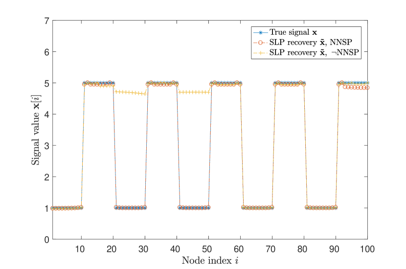
Fig. 2: Clustered graph signal $x[i]$ along with the recovered signals obtained from sampling sets $\mathcal{M}_{1}$ and $\mathcal{M}_{2}$.

IV-B Minnesota Roadmap

The second data set, with associated data graph $\mathcal{G}_{\rm min}$, represents the roadmap of Minnesota [5]. The data graph $\mathcal{G}_{\rm min}$ consists of $|\mathcal{V}|=2642$ nodes, and $|\mathcal{E}|=3303$ edges. We generate a clustered graph signal defined over $\mathcal{G}_{\rm min}$ by randomly selecting three different nodes $\{i_{1},i_{2},i_{3}\}$ which are declared as “cluster centres” of the clusters $\mathcal{C}_{1},\mathcal{C}_{2},\mathcal{C}_{3}$. The remaining nodes $\mathcal{V}\setminus\{i_{1},i_{2},i_{3}\}$ are then associated to the cluster whose centre is nearest in the sense of smallest geodesic distance. The edges connecting nodes within the same cluster have weight $W_{i,j}=4$, and those connecting different clusters have weight $W_{i,j}=2$.

We use SLP to recover the entire graph signal from its values obtained for the nodes in a sampling set. Two different choices $\mathcal{M}_{1}$ and $\mathcal{M}_{2}$ for the sampling set are considered: The sampling set $\mathcal{M}_{1}$ is based on the NNSP and consists of all nodes which are adjacent to the boundary edges between two different clusters. In contrast, the sampling set $\mathcal{M}_{2}$ is obtained by selecting uniformly at random a total of $|\mathcal{M}_{1}|$ nodes from $\mathcal{G}_{\rm min}$, i.e., we ensure $|\mathcal{M}_{1}|=|\mathcal{M}_{2}|$.

The resulting MSE is $0.0023$ for the sampling set $\mathcal{M}_{1}$ (conforming with NNSP), while the recovery using the random sampling set $\mathcal{M}_{2}$ incurred an average (over $100$ i.i.d. simulation runs) MSE of $0.0502$. In Figure 3, we depict the recovered graph signals using signal samples from either $\mathcal{M}_{1}$ or $\mathcal{M}_{2}$ (one typical realization). Evidently, the recovery using the sampling set $\mathcal{M}_{1}$ (which is guided by the NNSP) results in a more accurate recovery compared to using the random sampling set $\mathcal{M}_{2}$.

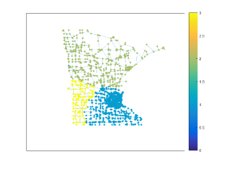
(a)

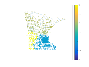
(b)

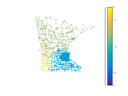
(c)

Fig. 3: True graph signal (a) and recovered signals for the Minnesota roadmap data set obtained (b) when using sampling set $\mathcal{M}_{1}$, (c) or sampling set $\mathcal{M}_{2}$ (Figure 3c).

V Conclusions

We considered the problem of recovering clustered graph signals, defined over complex networks, from observing its signal values on a small set of sampled nodes.

By extending tools from compressed sensing, we derived a sufficient condition, the network nullspace property (NNSP), on the graph topology and sampling set such that a convex recovery method is accurate. This condition is based on the connectivity properties of the underlying network. In particular, it requires the existence of certain network flows with the edge weights of the data graph being interpreted as capacities.

The NNSP involves both, the sampling set and the cluster structure of the data graph. Roughly speaking it requires to sample more densely near the boundaries between different clusters. This intuition has be verified by means of numerical experiments on synthetic and real-world datasets.

Our work opens up several avenues for future research. In particular, it would be interesting to analyze how likely the NNSP holds for certain random network models and sampling strategies. The tightness of the resulting recovery guarantees could then be contrasted with fundamental lower bounds obtained from an information-theoretic approach to minimax-estimation. Moreover, we would like to study variations of the SLP problem which are more suitable for classification problems.

VI Proofs

The proofs for Theorem 3 and Theorem 4 rely on recognizing the recovery problem (1) as an analysis $\ell_{1}$-minimization problem [24]. A sufficient condition for analysis $\ell_{1}$-minimization to deliver the correct solution $x[\cdot]$ is given by the analysis nullspace property [24, 20]. In particular, the sampling set $\mathcal{M}$ is said to satisfy the stable analysis nullspace property w.r.t. an edge set $\mathcal{S}\subseteq\mathcal{E}$ if

$$\|u[\cdot]\|_{\mathcal{E}\setminus\mathcal{S}}\geq\kappa\|u[\cdot]\|_{\mathcal{S}}\mbox{ for any }u[\cdot]\in\mathcal{K}(\mathcal{M}),$$ (9)

for some constant $\kappa>1$.

Lemma 5.

Consider a data graph $\mathcal{G}$ and fixed partitioning $\mathcal{F}=\{\mathcal{C}_{1},\ldots,\mathcal{C}_{|\mathcal{F}|}\}$ of its nodes into $|\mathcal{F}|$ clusters $\mathcal{C}_{l}$. We observe a clustered graph signal $x[\cdot]$ with $x[i]=\sum_{l=1}^{|\mathcal{F}|}a_{l}\mathcal{I}_{\mathcal{C}_{l}}[i]$ at the sampled nodes $\mathcal{M}\!\subseteq\!\mathcal{V}$. If (9) holds for $\mathcal{S}\!=\!\partial\mathcal{F}$, then (1) has a unique solution given by $x[\cdot]$.

Proof.

Consider a graph signal $\hat{x}[\cdot]$, which is different from the true underlying graph signal $x[\cdot]$, being feasible for (1), i.e, $\hat{x}[i]=x[i]$ for all sampled nodes $i\in\mathcal{M}$. Then, the difference $u[i]:=\hat{x}[i]-x[i]$ belongs to the kernel $\mathcal{K}(\mathcal{M})$ (cf. (4)). Note that, since $x[i]$ is constant for all nodes $i\in\mathcal{C}_{l}$ in the same cluster,

$$\hat{x}[i]-\hat{x}[j]=u[i]-u[j]\mbox{, for any edge }\{i,j\}\in\mathcal{E}\setminus\partial\mathcal{F}.$$ (10)

By the triangle inequality,

$$\|\hat{x}[\cdot]\|_{\partial\mathcal{F}} \geq\|x[\cdot]\|_{\partial\mathcal{F}}-\|u[\cdot]\|_{\partial\mathcal{F}}=\|x[\cdot]\|_{\rm TV}\!-\!\|u[\cdot]\|_{\partial\mathcal{F}},$$

and, since $\|\hat{x}[\cdot]\|_{\rm TV}=\|\hat{x}[\cdot]\|_{\partial\mathcal{F}}+\|\hat{x}[\cdot]\|_{\mathcal{E}\setminus\partial\mathcal{F}}$, in turn

$$\|\hat{x}[\cdot]\|_{\rm TV} \!=\!\|\hat{x}[\cdot]\|_{\partial\mathcal{F}}\!+\!\|\hat{x}[\cdot]\|_{\mathcal{E}\setminus\partial\mathcal{F}}\stackrel{{\scriptstyle\eqref{equ_supp_vx_edgesupport}}}{{=}}\|\hat{x}[\cdot]\|_{\partial\mathcal{F}}+u[\cdot]\|_{\mathcal{E}\setminus\partial\mathcal{F}}$$

$$\geq\|x[\cdot]\|_{\rm TV}\!-\!\|u[\cdot]\|_{\partial\mathcal{F}}\!+\!\|u[\cdot]\|_{\mathcal{E}\setminus\partial\mathcal{F}}\stackrel{{\scriptstyle\eqref{equ_NSP1}}}{{>}}\|x[\cdot]\|_{\rm TV}.$$

Thus, we have shown that any graph signal $\hat{x}[\cdot]$ which is different from the true underlying graph signal $x[\cdot]$ but coincides with it at all sampled nodes $i\in\mathcal{M}$, must have a larger TV norm than the true signal $x[\cdot]$ and therefore cannot be optimal for the problem (1). ∎

The next result extends Lemma 5 to graph signals $x[\cdot]\in\mathbb{R}^{\mathcal{V}}$ which are not exactly clustered, but which can be well approximated by a clustered signal of the form (2).

Lemma 6.

Consider a data graph $\mathcal{G}$ and a fixed partition $\mathcal{F}=\{\mathcal{C}_{1},\ldots,\mathcal{C}_{|\mathcal{F}|}\}$ of its nodes into disjoint clusters $\mathcal{C}_{l}\subseteq\mathcal{V}$. We observe a graph signal $\mathbf{x}\!\in\!\mathbb{R}^{\mathcal{V}}$ at the sampling set $\mathcal{M}\!\subseteq\!\mathcal{V}$. If (9) holds for $\mathcal{S}\!=\!\partial\mathcal{F}$ and $\kappa\!=\!2$, any solution $\hat{x}[\cdot]$ of (1) satisfies

$$\|x[\cdot]\!-\!\hat{x}[\cdot]\|_{\rm TV}\!\leq\!6\min_{a_{l}\in\mathbb{R}}\big{\|}x[\cdot]-\sum_{l=1}^{|\mathcal{F}|}a_{l}\mathcal{I}_{\mathcal{C}_{l}}[\cdot]\big{\|}_{\rm TV}.\vspace*{-2mm}$$ (11)

Proof.

The argument closely follows the proof of [19, Theorem 8]. First note that any solution $\hat{x}[\cdot]$ of (1) obeys

$$\|\hat{x}[\cdot]\|_{\rm TV}\leq\|x[\cdot]\|_{\rm TV},$$ (12)

since $x[\cdot]$ is trivially feasible for (1). From (12), we have

$$\|\hat{x}[\cdot]\|_{\mathcal{S}}\!+\!\|\hat{x}[\cdot]\|_{\mathcal{E}\setminus\mathcal{S}}\!\leq\!\|x[\cdot]\|_{\mathcal{S}}\!+\!\|x[\cdot]\|_{\mathcal{E}\setminus\mathcal{S}}.$$ (13)

Since $\hat{x}[\cdot]$ is feasible for (1), i.e., $\hat{x}[i]=x[i]$ for every sampled node $i\in\mathcal{M}$, the difference $v[\cdot]:=\hat{x}[\cdot]\!-\!x[\cdot]$ belongs to $\mathcal{K}(\mathcal{M})$ (cf. (4)). Applying the triangle inequality to (13),

$$\|v[\cdot]\|_{\mathcal{E}\setminus\mathcal{S}}\leq\|v[\cdot]\|_{\mathcal{S}}+2\|x[\cdot]\|_{\mathcal{E}\setminus\mathcal{S}}.$$ (14)

Combining (14) with (9) (for the signal $u[\cdot]=v[\cdot]$),

$$\|v[\cdot]\|_{\mathcal{E}\setminus\mathcal{S}}\leq 4\|x[\cdot]\|_{\mathcal{E}\setminus\mathcal{S}}.$$ (15)

Using (9) again,

$$\|x[\cdot]\!-\!\hat{x}[\cdot]\|_{\rm TV} =\|v[\cdot]\|_{\rm TV}=\|v[\cdot]\|_{\mathcal{S}}\!+\!\|v[\cdot]\|_{\mathcal{E}\setminus\mathcal{S}}$$

$$\stackrel{{\scriptstyle\eqref{equ_NSP1}}}{{\leq}}(3/2)\!\|v[\cdot]\|_{\mathcal{E}\setminus\mathcal{S}}\stackrel{{\scriptstyle\eqref{equ_offsupport_leq_fourtimes}}}{{\leq}}6\|x[\cdot]\|_{\mathcal{E}\setminus\mathcal{S}}.$$

For any clustered graph signal $x_{\rm c}[\cdot]$ of the form $x_{\rm c}[i]=\sum_{l=1}^{|\mathcal{F}|}a_{l}\mathcal{I}_{\mathcal{C}_{l}}[i]$, we have $x_{c}[i]\!-\!x_{c}[j]=0$ for any $\{i,j\}\in\mathcal{E}\setminus\mathcal{S}$ (note that $\mathcal{S}=\partial\mathcal{F}$) and, in turn,

$$\|x[\cdot]\!+\!x_{\rm c}[\cdot]\|_{\rm TV} =\!\|x[\cdot]\!+\!x_{\rm c}[\cdot]\|_{\mathcal{E}\setminus\mathcal{S}}+\|x[\cdot]\!+\!x[\cdot]_{c}\|_{\mathcal{S}}$$

$$\geq\|x[\cdot]\!+\!x[\cdot]_{c}\|_{\mathcal{E}\setminus\mathcal{S}}=\|x[\cdot]\|_{\mathcal{E}\setminus\mathcal{S}}.$$

∎

Let us now render Lemma 5 and Lemma 6 for clustered graph signals $x[\cdot]$ of the form (2) by stating a condition on the graph topology and sampling set $\mathcal{M}$ which ensures (9).

Lemma 7.

If a sampling set $\mathcal{M}$ satisfies NNSP-$\mathcal{F}$, then it also satisfies the stable analysis nullspace property (9).

Proof.

Consider a signal $u[\cdot]\!\in\!\mathcal{K}(\mathcal{M})$ which vanishes at all sampled nodes, i.e., $u[i]=0\mbox{ for all }i\in\mathcal{M}$. We will now show that $\|u[\cdot]\|_{\mathcal{E}\setminus\partial\mathcal{F}}\geq 2\|u[\cdot]\|_{\partial\mathcal{F}}$.

Let us assume that for each boundary edge $e\in\partial\mathcal{F}$, the flow $f[\cdot]$ in Definition 2 has the same sign as $u[e^{+}]-u[e^{-}]$. We are allowed to assume this since according to Definition 2, if there exists a flow with $f[e^{\prime}]>0$ for a boundary edge $e^{\prime}\in\partial\mathcal{F}$, there is another flow $\tilde{f}[\cdot]$ with $\tilde{f}[e^{\prime}]=-f[e^{\prime}]$ for the same edge $e^{\prime}\in\partial\mathcal{F}$, but otherwise identical to $f[\cdot]$, i.e., $\tilde{f}[e]=f[e]$ for all $e\in\mathcal{E}\setminus\{e^{\prime}\}$.

Next, we construct an augmented graph $\mathcal{G}^{\prime}$ by adding an extra node $s$ to the data graph $\mathcal{G}$ which is connected to all sampled nodes $i\in\mathcal{M}$ via an edge $e_{i}=\{s,i\}$ which is oriented such that $e_{i}^{+}=s$. We assign to each edge $e_{i}=\{s,i\}$ the flow $f[e_{i}]=g[i]$ (cf. (5)). It can be verified easily that the flow over the augmented graph has zero demands for all nodes. Thus, we can apply Tellegen’s theorem [27] to obtain $\|u[\cdot]\|_{\mathcal{E}\setminus\partial\mathcal{F}}\geq 2\|u[\cdot]\|_{\partial\mathcal{F}}$.

∎

We obtain Theorem 3 by combining Lemma 7 with Lemma 5. In order to verify Theorem 4 we note that, by Lemma 7, the NNSP according to Definition 2 implies the stable nullspace property (9) for $\mathcal{S}=\partial\mathcal{F}$. Therefore, we can invoke Lemma 6 to reach (8).

References

- [1] S. Basirian and A. Jung. Random walk sampling for big data over networks. In Proc. Int. Conf. Sampling. Th. and App. (SampTA), pages 427–431, Tallinn, Estonia, Jul. 2017.
- [2] A. Chambolle and T. Pock. A first-order primal-dual algorithm for convex problems with applications to imaging. J. Math. Imaging Vision, 40(1):120–145, May 2011.
- [3] O. Chapelle, B. Schölkopf, and A. Zien, editors. Semi-Supervised Learning. The MIT Press, Cambridge, Massachusetts, 2006.
- [4] S. Chen, R. Varma, A. Sandryhaila, and J. Kovačević. Discrete signal processing on graphs: sampling theory. IEEE Trans. Signal Processing, 63(24):6510–6523, Dec. 2015.
- [5] S. Chen, R. Varma, A. Sandryhaila, and J. Kovačević. Representations of piecewise smooth signals on graphs. In Proc. IEEE ICASSP 2016, Shanghai, China, March 2016.
- [6] S. Cui, A. Hero, Z.-Q. Luo, and J. Moura, editors. Big Data over Networks. Cambridge Univ. Press, 2016.
- [7] R. Diestel. Graph Theory. Springer, New York, 2000.
- [8] D. L. Donoho. Compressed sensing. IEEE Trans. Inf. Theory, 52(4):1289–1306, Apr. 2006.
- [9] Y. C. Eldar. Sampling Theory - Beyond Bandlimited Systems. Cambridge Univ. Press, Cambridge, UK, 2015.
- [10] S. Fortunato. Community detection in graphs. Physics Reports, 486:75–174, Feb. 2010.
- [11] S. Foucart and H. Rauhut. A Mathematical Introduction to Compressive Sensing. Springer, New York, 2012.
- [12] D. Gleich. MatlabBGL - A matlab graph library, 2007.
- [13] G. Hannak, P. Berger, G. Matz, and A. Jung. Efficient graph signal recovery over big networks. In Proc. Asilomar Conf. Signals, Systems, Computers, pages 1–6, Pacific Grove, CA, Nov. 2016.
- [14] A. Jung, P. Berger, G. Hannak, and G. Matz. Scalable graph signal recovery for big data over networks. In Proc. IEEE-SP Workshop on Sig. Proc. Adv. in Wireless Comm. (SPAWC), Edinburgh, UK, Jul. 2016.
- [15] A. Jung, A. Heimowitz, and Y. C. Eldar. The network nullspace property for compressed sensing over networks. In Proc. Int. Conf. Sampling Th. and App. (SampTA), Tallinn, Estonia, Jul. 2017.
- [16] A. Jung, A. O. Hero, III, A. Mara, and B. Jahromi. Semi-supervised learning via sparse label propagation. submitted to a journal. preprint available under https://arxiv.org/abs/1612.01414, May 2017.
- [17] A. Jung and M. Hulsebos. The network nullspace property for compressed sensing of big data over networks. arXiv, 2017.
- [18] A. Jung, N. Tran, and A. Mara. When is network lasso accurate? Frontiers in Applied Mathematics and Statistics, 3:28, Jan. 2018.
- [19] M. Kabanava and H. Rauhut. Analysis -recovery with frames and gaussian measurements. Acta Applicandae Mathematicae, 140(1):173 – 195, Dec. 2015.
- [20] M. Kabanava and H. Rauhut. Cosparsity in compressed sensing. In H. Boche, R. Calderbank, G. Kutyniok, and J. Vybiral, editors, Compressed Sensing and Its Applications, pages 315–339. Springer, 2015.
- [21] J. Kleinberg and E. Tardos. Algorithm Design. Addison Wesley, New York, 2006.
- [22] A. Mara and A. Jung. Recovery conditions and sampling strategies for network lasso. In Proc. Asilomar Conf. Signals, Systems, Computers, Pacific Grove, CA, Nov. 2017.
- [23] A. G. Marques, S. Segarra, G. Leus, and A. Ribeiro. Sampling of graph signals with successive local aggregation. IEEE Trans. Signal Processing, 64(7):1832–1843, Apr. 2016.
- [24] S. Nam, M. Davies, M. Elad, and R. Gribonval. The cosparse analysis model and algorithms. Applied and Computational Harmonic Analysis, 34(1):30–56, Jan. 2013.
- [25] J. Sharpnack, A. Rinaldo, and A. Singh. Sparsistency of the edge lasso over graphs. In Proc. 15th Int. Conf. on Artificial Intelligence and Statistics (AISTATS), La Palma, Canary Islands, Apr. 2012.
- [26] D. Spielman and S.-H. Teng. A local clustering algorithm for massive graphs and its application to nearly linear time graph partitioning. SIAM J. Comput., 42(1), Jan. 2013.
- [27] B. D. H. Tellegen. A general network theorem with applications. Philips Research Reports, 7:259–269, Feb. 1952.
- [28] Y.-X. Wang, J. Sharpnack, A. J. Smola, and R. J. Tibshirani. Trend filtering on graphs. J. Mach. Lear. Research, 17, Apr. 2016.
- [29] F. Zhao and L. J. Guibas. Wireless Sensor Networks: An Information Processing Approach. Morgan Kaufmann, Amsterdam, The Netherlands, 2004.
- [30] Y. Zhu. An augmented ADMM algorithm with application to the generalized lasso problem. Journal of Computational and Graphical Statistics, 26(1):195–204, Feb. 2017.