CME Dynamics Using STEREO and LASCO Observations: The Relative Importance of Lorentz Forces and Solar Wind Drag

1 Introduction

S-Introduction Coronal mass ejections (CMEs) from the Sun are generally acknowledged as the main cause of disturbances in the near-Earth space environment. Due to the considerable technological impacts caused by such disturbances, it has become increasingly important to study and understand various aspects related to CME impacts on the Earth’s magnetosphere (Gosling et al., 1991; Bothmer and Daglis, 2007). One of the most basic quantities in this regard concerns the time it takes for a CME to reach the Earth after it has been detected leaving the Sun using space-based coronagraphs; This quantity is called the Sun – Earth travel time. Among the factors that affect the travel time are the CME size, mass, initial velocity and the ambient solar wind speed (Bosman et al., 2012). An accurate and reliable forecast of the Sun – Earth travel time is obviously important to a space weather mitigation framework, as is a good estimate of the expected speed of the CME near the Earth. These quantities are typically computed from a dynamical model for CME propagation, that uses near-Sun coronagraph observations as input.

The basic outlines of such dynamical CME propagation models have been well established for a while. One dimensional (1D) models that incorporate Lorentz force driving, aerodynamic drag, and other effects have been in vogue since 1996 (e.g. Chen, 1996; Kumar and Rust, 1996). So-called drag-based models (DBM), which consider only aerodynamic drag, have been very popular lately (e.g. Cargill, 2004; Vršnak et al., 2010; Mishra and Srivastava, 2013; Temmer and Nitta, 2015). More sophisticated three dimensional (3D) MHD models such as ENLIL (e.g. Taktakishvili et al., 2009; Lee et al., 2013; Vršnak et al., 2014; Mays et al., 2015), global MHD model using the data-driven Eruptive Event Generator Gibson-Low (EEGGL) (e.g. Jin et al., 2017), CME and shock propagation models like the Shock Time of Arrival Model (STOA), the Interplanetary Shock Propagation model (ISPM) and the Hakamada-Akasofu-Fry version 2 model (e.g. Fry et al., 2003; McKenna-Lawlor et al., 2006), other hybrid models (Wu et al., 2007) and the Space Weather Modeling Framework (SWMF; Lugaz et al., 2007; Tóth et al., 2007) are also often used in modeling CME propagation.

Despite considerable progress, our ability to successfully model the Sun – Earth travel time and the near-Earth speed of Earth-directed CMEs is still limited (Zhao and Dryer, 2014), even for relatively simple events that do not involve interacting CMEs (e.g. Temmer et al., 2012). Part of the reason for this is that the models are still largely empirical. For instance, most drag-based models use the dimensionless drag coefficient $C_{\rm D}$ and/or the parameter $\gamma$ (ratio of drag acceleration and square of the difference between the CME and solar wind speeds) as a fitting parameter. The physical basis of the aerodynamic drag experienced by CMEs is only starting to be understood (Subramanian, Lara, and Borgazzi, 2012; Sachdeva et al., 2015). As far as Lorentz forces go, it is also generally thought that they are dominant only in the initial phases of CME propagation, when they are relatively near the Sun. However, for a given CME, its not clear where Lorentz forces peak and when they cease to be important. Some 1D models (e.g. Chen and Kunkel, 2010; Zhang et al., 2001) assume that the Lorentz force follows the temporal profile of the soft X-ray flare that often accompanies the CMEs.

In this article we adopt the physical definition for CME aerodynamic drag outlined in Sachdeva et al. (2015), referred to as Paper 1 from now on, together with a specific model (Kliem and Török, 2006) for Lorentz forces to address some of these questions: What is the heliocentric distance range where Lorentz forces dominate? Beyond what heliocentric distance is a drag-only model justified? The rest of the article is organized as follows. In Section S-f we discuss the forces affecting the CME propagation. Section S-data provides details of the CME event sample and data obtained from Graduated Cylindrical Shell (GCS) fitting. The analysis and main results are outlined in Section S-res, followed by discussion and conclusions in Section S-conc.

2 Forces Acting on CMEs

S-f

Descriptions of CME evolution usually consider an initiation phase comprising the initial CME eruption, which is followed by the propagation phase. There is an interplay between Lorentz forces, gravity and solar wind aerodynamic drag in the propagation phase; this provides the residual acceleration (e.g. Zhang and Dere, 2006; Subramanian and Vourlidas, 2007; Gopalswamy, 2013). Gravitational forces and plasma pressure are generally taken to be negligible for flux rope models of CMEs (Forbes, 2000; Isenberg and Forbes, 2007). Lorentz forces are thought to accelerate CMEs up to a few solar radii in the low corona (e.g. Vršnak, 2006; Bein et al., 2011; Carley, McAteer, and Gallagher, 2012), beyond which the solar wind aerodynamic drag takes over. Paper 1 shows that aerodynamic drag accounts for the observed CME trajectory only beyond 15 – 50 R_⊙ for the slow (near-Sun speeds $<900$ km s^-1) CMEs; for fast CMEs (near-Sun speed $>900$ km s^-1), aerodynamic drag can account for their dynamics from 5 R_⊙ onwards. Rollett et al. (2016) also show that their Drag-based model(DBM) is applicable only beyond a heliocentric distance of 21$\pm$10 R_⊙.

The forces acting on a CME are often represented in the following form (in cgs units):

$$F\, = m_{cme}\frac{d^{2}R}{dt^{2}}$$ (1)

$$= F_{\rm Lorentz}+F_{\rm drag}$$

$$= \biggl{\{}\biggl{[}\frac{\pi I^{2}}{c^{2}}\biggl{(}ln\biggl{(}\frac{8R}{b}\biggr{)}-\frac{3}{2}+\frac{l_{i}}{2}\biggr{)}\biggr{]}\,-\,\frac{(\pi R)IB_{ext}(R)}{c}\biggr{\}}$$

$$-\,\,\frac{1}{2}\,\,C_{\rm D}\,\,A_{cme}\,\,n_{sw}\,\,m_{p}\,\bigl{(}V_{cme}-V_{sw}\bigr{)}\,\,\bigl{|}V_{cme}-V_{sw}\bigr{|}$$

where $F$ is the total force, $m_{\rm cme}$ is the CME mass, $R$ is the heliocentric distance of the leading edge of the CME (also often interpreted as the position of the center of mass) and t represents time. $F_{\rm Lorentz}$ is the net Lorentz force acting on the CME in the major radial direction which is given by the term in the curly brackets (see e.g. Shafranov, 1966; Kliem and Török, 2006). The first term (within the square braces) represents the Lorentz self forces ($(1/c)J\times B$, where $J$ is the current density and $B$ the magnetic field) acting on the expanding CME current loop (e.g. Chen, 1989) that accelerate the CME while the second term is the force due to the external poloidal field ($B_{ext}$) that tends to hold down the expanding CME. In the equation, $I$ is the CME current, $c$ is the speed of light, $b$ is CME minor radius and $l_{i}$ is the internal inductance. The axial current, $I$, is determined by the conservation of total (i.e. flux-rope + external) magetic flux.

The term in Equation (eqf) involving $C_{\rm D}$ represents the aerodynamic drag experienced by the CME as it propagates through the solar wind. The strength of the momentum coupling between the CME and the solar wind is represented by the dimensionless drag coefficient, $C_{\rm D}$. We use a non-constant $C_{\rm D}$ given by Equation 7 of Paper 1. For completeness, we include the $C_{\rm D}$ definition here:

$$C_{\rm D}=0.148-4.3\times 10^{4}\,Re^{-1}+9.8\times 10^{-9}\,Re\,,\ilabel{eqcdfit}$$ (2)

where Re is the Reynolds number calculated using the solar wind viscosity expression as described in Paper 1. The quantity $A_{\rm cme}$ is the cross sectional area of the CME, $n_{sw}$ is the solar wind density, and $m_{p}$ is the proton mass. $V_{\rm cme}$ and $V_{\rm sw}$ denote the CME and solar wind velocities, respectively. Depending on how fast or slow a CME is travelling (relative to the solar wind), the solar wind can either “drag down” the CME or “pick it up”. Paper 1 finds that fast CMEs (initial velocity $\sim 916$ km s^-1) are governed primarily by aerodynamic drag from as early as $\sim 5.5$ R_⊙. On the other hand, slower CMEs are governed by solar wind aerodynamic drag only above 15 – 50 R_⊙.

In this article we analyze a diverse sample of 38 well observed CMEs. Using measurements with the Graduated Cylindrical Shell (GCS) method for each CME, we determine the heliocentric distance, $\widetilde{h}_{0}$, above which the CME dynamics is dominated by aerodynamic drag. Using the torus instability (TI) model to describe the Lorentz forces (Kliem and Török, 2006), we address questions such as: Where does the Lorentz force peak?, How does the Lorentz force compare with the aerodynamic drag force at and beyond $\widetilde{h}_{0}$? and more.

3 CME Data Sample

S-data

3.1 Event Selection

We investigate CMEs observed during the rising phase of Solar Cycle 24 between 2010 and 2013. The primary data we use is from the Large Angle Spectrometric Coronagaph (LASCO: Brueckner et al., 1995) onboard the Solar and Heliospheric Observatory mission (SOHO) and Sun – Earth Connection Coronal and Heliospheric Investigation (SECCHI: Howard et al., 2008) coronagraphs and the Heliospheric Imagers (HI) onboard the Solar TErrestrial RElations Observatory mission (STEREO; Kaiser et al., 2008). In-situ measurements are obtained from the Wind spacecraft, which gives the near-Earth parameters for these CMEs. The 38 CMEs we identify for this work have near-Sun speeds ranging from 50 km${\rm s}^{-1}$ to 2400 km${\rm s}^{-1}$. Of these, 13 events are partial halo (PH) CMEs and 21 are full halo(FH) CMEs as indicated in the SOHO/LASCO CME Catalog. The remaining four events have angular width $<120^{\circ}$. All the CMEs in our sample are Earth-directed. The respective separations of the STEREO B and A spacecraft from the Earth vary from 71^∘ and 66^∘ in March 2010 to about 149^∘ and 150^∘ by the end of 2013. Along with the LASCO C2 coronagraph, the three point view provides a favourable set up for observing Earth-directed CMEs. We only include CMEs that have continuous observations in LASCO C2, STEREO-A and -B COR 2, HI1 and HI2. We require that the images from all the instruments must include the CMEs as clear, bright structures. Events with major distortions and CME – CME interactions were excluded.

3.2 GCS Fitting

Needless to say, precise information about the 3-dimensional (3D) evolution of CMEs is central to building a good model. Early efforts in this direction include those of Chen et al. (1997) and Wood et al. (1997). The advent of SECCHI/STEREO data facilitated this task greatly. We use the Graduated Cylindrical Shell (GCS: Thernisien, Howard, and Vourlidas, 2006; Thernisien, Vourlidas, and Howard, 2009; Thernisien, 2011) model to fit the visible CME structure. Table tbl1 lists the GCS fitting parameters for all the CMEs. The serial number of each CME in Table tbl1 will be used as a reference to the corresponding event hereafter. The eight events from Paper 1 (marked with an asterisk $\ast$) have observations up to the HI2 field of view (FOV), while the remaining events have been fitted up to the HI1 FOV. The second and third columns in Table tbl1 indicate the CME event date and time of the first observation in the LASCO C2 FOV. The quantity $h_{0}$ is the height of the leading edge of the CME from the GCS fitting technique, at the time of first observation . The CME initial speed $v_{0}$ at $h_{0}$ is calculated by fitting a third-degree polynomial to the height-time observations. The quantities $n_{wind}$ and $v_{wind}$ are the proton number density and solar wind velocity at 1 AU as observed in-situ by the Wind spacecraft. These observed values are extrapolated sunward for use in $F_{\rm drag}$ for calculating $n_{sw}$ and $V_{sw}$ in Equation eqf. We follow the detailed description given in Paper 1 to calculate of various parameters, such as, $A_{cme}$, $n_{sw}$, $V_{sw}$, and $C_{\rm D}$ required in evaluating $F_{\rm drag}$.

GCS parameters like Carrington longitude, $\phi$, and heliographic latitude, $\theta$, along with the tilt, $\gamma$, provide details of the position of the source region (SR) and the orientation of the propagating CME. The quantity $\kappa$ is the aspect ratio and $\alpha$ is half of the angle between the axes and the legs of the flux-rope. Using the GCS fitted height of the leading edge ($R$), $\kappa$, and $\alpha$ at each time instant, other geometrical parameters like CME minor radius, $b$, ratio, $R/b$, elliptical cross-sectional width, and CME area, $A_{cme}$, are calculated (Thernisien, 2011) to be used in Equation eqf. The observed height-time data for each CME in our sample is thus derived from the GCS fitting of images at each time stamp.

Our sample includes 38 CMEs with an initial velocity range $47<v_{0}<2400$ km s^-1. There are 18 CMEs with initial velocities $v_{0}>900$ km s^-1. We call these events “fast” and indicate them by a superscript (f) in Tables tbl1 and tbl2. The fastest event is CME 23 on 27 January 2012, with $v_{0}\sim 2400$ km s^-1. The remaning 20 CMEs in the sample having $v_{0}<900$ km s^-1 are called “slower” CMEs.

4 Analysis and Results

S-res Our main aim in this article is to determine the heliocentric distance range(s) where the Lorentz force terms and the aerodynamic drag terms (Equation eqf) are respectively dominant.

4.1 Aerodynamic Drag

We first try to reconcile the observed CME dynamics with a solar wind aerodynamic drag-only model following the procedure described in Paper 1. In other words, we consider only the $F_{\rm drag}$ term in Equation eqf using observationally derived parameters and compare the model solutions with the observed height-time data. We find that the drag-only model solutions agree reasonably well with the observed CME profile right from the first data point ($h_{0}$) for the fast CMEs (initial velocity $>900$ km s^-1). Figure fig1 shows the height-time plot for CME 18 ($v_{0}\sim 1276$ km s^-1) and CME 36 ($v_{0}\sim 1217$ km s^-1), to compare the model results (red dash-dotted line) and data (diamonds). It is clear that for both these CMEs, solar wind drag explains the observed trajectory quite well from 4 and 4.9 R_⊙ onwards, respectively. This result is representative of all the 18 fast CMEs in our sample. However, this is not true for slower CMEs. Figure fig2 shows the results for two representative slower CMEs (CME 8, $v_{0}\sim 276$ km s^-1 and CME 29, $v_{0}\sim 461$ km s^-1) with the drag-only model initiated from the first observation point. The disagreement between the data (diamond symbols) and predicted solution (red dash-dotted line) is obvious, and indicates that the drag-only model, when initiated from the first data point, provides a poor explanation for the observed CME dynamics for slower CMEs. As in Paper 1, we then initiate the drag-only model at progressively later heights (using observational inputs appropriate to the initiation height). The initiation height at which the drag solution matches the observations is denoted by $\widetilde{h}_{0}$ in Table tbl2. The model predicted solution (denoted by a solid blue line) shown in Figure fig2 indicates that the drag-only model initiated above $\widetilde{h_{0}}$ ($\sim$ 21 and 31 R_⊙ for CME 8 and 29 respectively) provides a good description of the dynamics of these relatively slower CMEs. We follow this procedure for each event in our sample. The quantities $\widetilde{h}_{0}$ and corresponding velocity $\widetilde{v}_{0}$ are listed for each event in Table tbl2. We use the coefficient of determination (often called $R$ squared) to determine how well the predicted model solutions fit the data. Model solutions with $R^{2}>98\%$ are considered acceptable. The CME dynamics can be considered to be dominated by solar wind aerodynamic drag above the height $\widetilde{h}_{0}$. The left panel of Figure fig33 shows a plot of $\widetilde{h}_{0}$ (Table tbl2) versus the CME initial velocity ($v_{0}$). We see that for CMEs with $v_{0}<900$ km s^-1, $\widetilde{h}_{0}$ lies between 12 – 50 R_⊙ while for CMEs with $v_{0}>900$ km s^-1, $\widetilde{h}_{0}$ is same as the initial observed height for the event ($h_{0}$ in Table tbl1, which ranges from 3.9 – 8.4 R_⊙ for the fast CMEs in our sample). In other words, Figure fig33 shows that fast CMEs are drag-dominated from 3.9 – 8.4 R_⊙ onwards, while slower CMEs are drag dominated only beyond 12 – 50 R_⊙.

4.2 Lorentz Forces

If the aerodynamic drag dominates for heliocentric distances $R>\widetilde{h}_{0}$ (i.e. it is not necessary to invoke Lorentz forces to explain their dynamics), it is natural to investigate the behavior of Lorentz forces for $R<\widetilde{h}_{0}$. The first two terms in Equation eqf are a feature of most Lorentz force models that deal with CME initiation. All such models predict that the (total) Lorentz force increases until it peaks at a certain heliocentric distance, beyond which it decreases and becomes negligible. Some models tailor the injected poloidal flux (or equivalently, the driving current) so as to achieve this Lorentz-force profile (Chen and Kunkel, 2010). Others, such as the torus instability model (Kliem and Török, 2006) rely on the fact that the external Lorentz forces need to decrease (with heliocentric distance) faster than a certain rate, in order to “launch” the CME. This also results in a Lorentz-force profile that increases initially and achieves a peak before decreasing. Kliem et al. (2014) have also shown the equivalance of TI and the catastrophe mechanism for CME eruption (Forbes and Isenberg, 1991).

In this description, the equilibrium position of the flux rope, $h_{eq}$, is defined by a balance between the Lorentz self force and the external force. For the sake of concreteness, we adopt $h_{eq}=1.05$ R_⊙ in our work. The equilibrium position is also defined by an equilibrium current, $I_{eq}$. The current carried by the flux rope at a given $R$ is defined by (Kliem and Török, 2006):

$$I\,=\,\frac{c^{{}^{\prime}}_{eq}I_{eq}h_{eq}}{c^{{}^{\prime}}R}\biggl{(}1+\frac{(c^{{}^{\prime}}_{eq}+\frac{1}{2})}{2c^{{}^{\prime}}_{eq}(2-n)}\biggl{[}\biggl{(}\frac{R}{h_{eq}}\biggr{)}^{2-n}-1\,\biggr{]}\biggr{)}\,,\ilabel{eqI}$$ (3)

where $c^{{}^{\prime}}(R)\,=\,\bigl{[}ln(8R/b)-2+l_{i}/2\bigr{]}$ and $c^{{}^{\prime}}_{eq}\,=\,c^{{}^{\prime}}(R=h_{eq})=\bigl{[}ln(8h_{eq}/b_{eq})-2+l_{i}/2\bigr{]}$. The quantity $b$ is the flux rope minor radius. The external (ambient) magnetic field is $\propto R^{-n}$, and $n$ needs to be greater than a certain critical value for the torus instability to be operative, causing the flux rope to erupt. The quantity $l_{i}$ is the internal inductance of the flux rope, and we use $l_{i}=1/2$. The equilibrium current, $I_{eq}$, carried by the flux rope is related to the external field $B_{\rm ext}(h_{eq})$ at the equilibirum position via

$$I_{eq}\,=\,\frac{B_{\rm ext}(h_{eq})h_{eq}c}{c^{{}^{\prime}}_{eq}+\frac{1}{2}}\,\,.$$

For a given value of $n$, the value of $I_{eq}$ (and equivalently $B_{\rm ext}(h_{eq})$) is determined by the condition $F_{\rm drag}(\widetilde{h}_{0})=F_{\rm Lorentz}(\widetilde{h}_{0})$. It constrains the equilibrium current $I_{eq}$ and $n$. For a given event, $n$ is chosen to be the minimum value that will ensure that $|F_{\rm drag}|>F_{\rm Lorentz}$ for $R>\widetilde{h}_{0}$.

Table tbl2 gives the values of the equilibrium current $I_{eq}$ and $B_{ext}(h_{eq})$ for all CMEs for the corresponding value of the decay index n. The GCS fits to our observations yield values for the flux rope aspect ratio $R/b$. For heliocentric distances below the first observed point $h_{0}$ (which is typically around 3 R_⊙), we assume that $R/b$ is the same as the observed value at the first observed point ($h_{0}$). In other words, we assume that the flux rope expands in a self-similar manner from $h_{eq}$ to $h_{0}$; beyond $h_{0}$, we do not have to rely on any such assumption, since we have access to the observed values of $R/b$.

4.3 Lorentz Force versus Aerodynamic Drag

As an example, we show a plot of the Lorentz force versus heliocentric distance for CMEs 18 and 36 in Figure fig3 and CMEs 8 and 29 in Figure fig4. The red solid line indicates the points between $h_{eq}$ and $h_{0}$ where we do not have data for $R/b$ (in this region we assume that $R/b$ is the same as its value at $h_{0}$) and black diamonds indicate points for which we have observationally determined values for $R/b$. Clearly, the Lorentz force on the flux rope increases from its value at $h_{eq}$ to reach a peak at $h_{peak}$, after which it decreases. For each CME, the position at which the Lorentz force peaks ($h_{peak}$) is given in Table tbl2. The peak is generally between 1.65 and 2.45 R_⊙ for the CMEs in our sample. The green circles in Figures fig3 and fig4 indicate the absolute value of solar wind drag force with height above $\widetilde{h_{0}}$. The location of $\widetilde{h_{0}}$ is indicated by a blue dashed vertical line. The quantity marked “$Fall\,\%$” in Table tbl2 quantifies the amount by which the Lorentz force at $\widetilde{h_{0}}$ has fallen from its peak value at $h_{peak}$. For both the fast CMEs, CME 18 (left panel) and CME 36 (right panel) in Figure fig3, the Lorentz force peaks at 1.95 R_⊙ with $n=2.1$. The Lorentz force falls by 35 $\%$ for CME 18 and by 48 $\%$ for CME 36 from $h_{peak}$ up to $\widetilde{h}_{0}$; for these fast CMEs, $\widetilde{h}_{0}$ happens to be the same as $h_{0}$. For the slower CMEs (CME 8 and CME 29, shown in Figure fig4), $n=1.6$ and the Lorentz force peaks at 2.35 R_⊙ for both CMEs. The Lorentz force decreases by as much as 77 $\%$ from its value at $h_{peak}$ by $\widetilde{h}_{0}=20.8$ R_⊙, beyond which the solar wind drag takes over for CME 8. Similarly, for CME 29, the Lorentz force decreases by 79 $\%$ from $h_{peak}$ up to $\widetilde{h}_{0}=31$ R_⊙. This is typical of slower CMEs; for all the slower CMEs in Table tbl2, the Lorentz force at $\widetilde{h}_{0}$ (which is 12 – 50 R_⊙) has fallen by around 70-98 $\%$ from its peak value. While the Lorentz forces peak fairly early on ($h_{peak}\approx$ 1.65 – 2.45 R_⊙) for slow(er) CMEs, this means that they become negligible only as far out as 12 – 50 R_⊙.

For all the CMEs in our sample, the right panel of Figure fig33 shows the percentage by which the Lorentz force has fallen at $\widetilde{h}_{0}$ (relative to its peak value) as a function of the CME initial speed. Slower CMEs are denoted by blue circles and fast ones by black circles. The $Fall\,\%$ is clearly larger for the slower CMEs. Since the fast CMEs are drag dominated from relatively early on (left panel of Figure fig33), the $Fall\,\%$ is relatively lower.

Reiterating the results summarized in Table tbl2. Column 1 indicates the CME serial number corresponding to the events listed in Table tbl1. Column 2 lists the height $\widetilde{h}_{0}$ above which the solar wind drag dominates the CME dynamics. For slow CMEs, this height lies in the range 12 – 50 R_⊙ while for faster events it is the same as $h_{0}$ in Table tbl1. $\widetilde{v}_{0}$ is the CME speed at height $\widetilde{h}_{0}$. The values of $n$ in column 4 represent the decay index for each CME and lie between 1.6 and 3. We note that the fastest CMEs typically have the highest values for $n$. The quantity $h_{peak}$ quoted in column 5 gives the position where the Lorentz force peaks; it ranges between 1.65 and 2.45 R_⊙. The equilibrium current, $I_{eq}$, in column 6 is in units of $10^{10}$ A. The $I_{eq}$ estimates are in agreement with the average axial current calculated by Subramanian and Vourlidas (2007). The quantity $B_{ext}(h_{eq})$ in column 7 is the equilibrium magnetic field at $h_{eq}=1.05$ R_⊙ in units of G. $Fall\,\%$ in column 8 describes the amount by which the Lorentz force at $\widetilde{h}_{0}$ has decreased relative to its peak value. For slow CMEs, the percentage fall is between 70 – 98 $\%$ while for faster CMEs, it is between 20 – 60 $\%$. The last column indicates the quantity $F_{\rm diff}\,=\,((F_{\rm drag}-F_{\rm Lorentz})/F_{\rm drag})\times 100\%$ evaluated at 40 R_⊙ (except for CME 11, where it is evaluated at 50 R_⊙).

5 Discussion and Conclusions

S-conc

5.1 Discussion

Our main aim in this paper is to quantify the relative contributions of Lorentz forces and solar wind aerodynamic drag on CMEs as a function of heliocentric distance. Since these are the two main forces thought to be responsible for CME dynamics, it is essential to know their relative importance to build reliable models for CME Earth arrival time and speed. It is known that aerodynamic drag dominates CME dynamics only beyond distances as large as 15 – 50 R_⊙ for all but the fastest CMEs (Paper 1). This trend has also been confirmed by independent studies using an empirical fitting parameter for aerodynamic drag (e.g. Temmer et al 2015). One would assume that Lorentz forces are dominant below these heliocentric distances (and negligible above it), but this has not been explicitly confirmed so far. To the best of our knowledge, this is the first systematic study in this regard using a diverse CME sample.

We use a sample of 38 CMEs that are well observed by the SECCHI coronagraphs and the heliospheric imagers onboard STEREO and the LASCO coronagraphs onboard SOHO. We use detailed geometrical parameters from GCS fitting to the CMEs. Our prototypical models for aerodynamic drag and Lorentz forces are shown in Equation eqf. The model for aerodynamic drag follows the physical definition outlined in Paper 1, and the model for Lorentz forces follows the TI model of Kliem and Török (2006). Using only the aerodynamic drag term, we compute the heliocentric distance $\widetilde{h}_{0}$ beyond which solar wind drag can be considered to be the only force influencing the CME dynamics. This calculation makes use of several observational inputs for each CME: the ambient solar wind density and velocity, GCS fitted height, velocity and area for each CME. Subsequently, we use only the Lorentz force term. Using observational data for the aspect ratio of the CME flux rope, we determine the heliocentric distance $h_{peak}$ at which the Lorentz force attains its peak value. We also determine the percentage by which the Lorentz force decreases from its peak value at $h_{peak}$ up to $\widetilde{h}_{0}$ (beyond which aerodynamic drag becomes the dominant force). Table tbl2 summarizes all our results.

Some of the trends revealed by our results are depicted graphically in Figures fig33, fig7, and fig8. Blue circles indicate slow CMEs while the black circles represent fast events. As discussed earlier, Figure fig33 shows that aerodynamic drag dominates the dynamics of fast CMEs from a few R_⊙ onwards, whereas it is dominant for slow CMEs only beyond 12 – 50 R_⊙.

Figure fig7a shows the first observed height, $h_{0}$, of each CME as a function of its initial speed $v_{0}$. There does not seem to be a definite distinction between fast and slow CMEs in this regard. It is possible, however, that the limited time cadence of the LASCO C2 coronagraphs affects the values of $h_{0}$ for fast CMEs. We note that the first observed height for about 60 $\%$ of the CMEs lies between 2.9 and 5.0 R_⊙.

As depicted in Figures fig3 and fig4, the Lorentz force profile shows a steep increase from $h_{eq}$ until it peaks at $h_{peak}$, beyond which it decreases. Figure fig7b is a scatterplot of the position of the Lorenz force peak ($h_{peak}$, see Table tbl2) as a function of the CME initial speed, $v_{0}$. The value of $h_{peak}$ is between 1.65 and 2.45 R_⊙ for all CMEs, with no noticeable trend distinguishing slow and fast ones.

As shown in the right panel of Figure fig33, the percentage decrease, $Fall\,\%$, of the Lorentz force at $\widetilde{h}_{0}$ (relative to its value at $h_{peak}$) is considerably higher for slow CMEs than it is for fast ones. Figure fig7c shows a different way of visualising this data - the quantity $Fall\,\%$ is plotted as a function of $\widetilde{h}_{0}$. It shows that the percentage decrease is larger for CMEs with larger $\widetilde{h}_{0}$ (the slow ones) than it is for those with relatively smaller values of $\widetilde{h}_{0}$ (the fast ones).

The drag-only model accounts well for the CME trajectory when initiated at $\widetilde{h}_{0}$ (or beyond). This implies that other forces (such as Lorentz forces) are not important beyond this height. We find this to be true for 36 of the 38 CMEs in our sample. CMEs 4 and 10 (which are slow) are the only exceptions. However, we find that the difference between the drag force and the Lorentz force beyond $\widetilde{h}_{0}$ is much more pronounced for fast CMEs than for slow ones (e.g. Figures fig3 and fig4). In order to quantify this, we compute the quantity $F_{\rm diff}\,=\,100\times(F_{\rm drag}-F_{\rm Lorentz})/F_{\rm drag}$ for all the CMEs in our list. This quantity is plotted in Panel a of Figure fig8 as a function of the CME initial velocity $v_{0}$; as before, blue circles represent slow CMEs while black ones represent fast ones. We show the relative percentage difference for all events at 40 R_⊙ except for CME 11. Since $\widetilde{h}_{0}\sim 46$ R_⊙ for CME 11, $F_{\rm diff}$ is evaluated at 50 R_⊙ for this event. The drag force is 50 – 90% larger at 40 R_⊙ than the Lorentz force for most of the fast events. This justifies the success of the drag-only model for fast events. On the other hand, this number ranges from 0.2% and 30% for the slower events. Evidently, for some of the slower CMEs, the computed Lorentz force is only slightly smaller than the drag force, even well beyond $\widetilde{h}_{0}$. For the slow CMEs 4 and 10, the Lorentz force is in fact larger than the solar wind drag force in magnitude. Figure fig8b shows a plot of the absolute magnitude of the solar wind drag force (in units of $10^{17}$ dyn) for all CMEs at $\widetilde{h}_{0}$ versus the CME initial velocity, $v_{0}$. Since a drag-only model describes the data well for all the events in our list, it follows that the Lorentz force we compute for some of the slower CMEs is an over-estimate. Our Lorentz force computations assume that the total magnetic flux is frozen in. The time evolution of the enclosed current $I$, follows from this assumption. However, this assumption might not be accurate - some of the magnetic energy might be expended in CME expansion and/or heating of the CME plasma. Our results suggest that such effects might be especially important for slower CMEs.

5.2 Conclusions

Our main conclusions are:

• Our analysis shows that a model that includes only the solar wind aerodynamic drag accurately describes the trajectory of fast CMEs from very early on. The converse is true for slower CMEs. The distance $\widetilde{h}_{0}$ beyond which the solar wind aerodynamic drag dominates over Lorentz forces can be as small as 3.5 – 4 R_⊙ for fast ($>900$ km s^-1) CMEs, and as large as 12 – 50 R_⊙ for slower ones (47 – 890 km s^-1).

• The distance $h_{peak}$ at which the Lorentz force peaks is between 1.65 and 2.45 R_⊙ for all CMEs.

• At $\widetilde{h}_{0}$, the Lorentz force has typically fallen by 20 – 60 % (relative to its peak value) for fast CMEs. For slower CMEs, the decrease ranges between 70 – 98%.

• Well beyond $\widetilde{h}_{0}$, the drag force exceeds the Lorentz driving force by a significant amount for fast CMEs (50% – 90%). However, for some slow CMEs the dominance of the drag force is not as pronounced, suggesting that part of the CME’s magnetic flux may be dissipated in aiding its expansion or heating.

In calculating the Lorentz force, the initial equilibrium position for the CME flux rope is is taken to be $h_{eq}$ = 1.05 R_⊙ for all events. The overlying field is taken to decrease as $B_{ex}\propto R^{-n}$. The quantity $n$ needs to be greater than a critical value $n_{cr}$ ($n_{cr}=3/2-1/(4c^{{}^{\prime}}_{eq})$) for the torus instability to be operative, ensuring CME eruption. For each CME, we choose a value of $n$ that is $>n_{cr}$. We demand that the Lorentz force equals the aerodynamic drag force at $\widetilde{h}_{0}$. The value for $n$ is chosen such that the Lorentz force remains lower than the aerodynamic drag force beyond $\widetilde{h}_{0}$. For the CMEs in our sample, the critical decay index $n_{cr}$ ranges from 1.29 to 1.39.

For a fixed value of $n$, we note that an increase in $h_{eq}$ by 14 $\%$ increases the peak force position value by $\sim 15\%$. It decreases the $Fall\,\%$ of the Lorentz force at $\widetilde{h}_{0}$ (relative to its peak value) by 5 $\%$. For a fixed value of $h_{eq}(-1.05$ R${}_{\odot})$, an increase in n by $31\%$ decreases the peak position by 17 $\%$. It also increases the $Fall\,\%$ of the Lorentz force at $\widetilde{h}_{0}$ (relative to its peak value) by 19.5 $\%$.

Although we have considered only Lorentz and solar wind aerodynamic drag in order to explain CME dynamics, we note that there can be other important contributors to the overall energetics. For instance, the work involved in CME expansion and the energy expended in possibly heating the CME plasma e.g. Kumar and Rust (1996); Wang, Zhang, and Shen (2009); Emslie et al. (2012) are not considered here. These could well be important, in addition to the energy dissipated due to aerodynamic drag. An understanding of these quantities can be achieved via observations of CME expansion as well as measurements of thermodynamic quantities inside the CME as it progresses through the heliosphere. The latter can possibly be done with the upcoming Solar Probe Plus and Solar Orbiter missions or via an off-limb spectroscopy mission.

Acknowledgements: NS acknowledges support from a PhD studentship at IISER Pune, from NAMASTE India-EU scholarship and from the Infosys Foundation Travel Award. NS is thankful to A. Pluta and N. Mrotzek for their help and useful discussions about data selection and fitting procedures. PS acknowledges support from the Indian Space Research Organization via a RESPOND grant. AV is supported by NNX16AH70G. VB acknowledges support of the CGAUSS (Coronagraphic German and US Solar Probe Plus Survey) project for WISPR by the German Space Agency DLR under grant 50 OL 1601. The SECCHI data are produced by an international consortium of the NRL, LMSAL and NASA/GSFC (USA), RAL and Univ. Bham (UK), MPS (Germany), CSL (Belgium), IOTA and IAS (France).

Table 1.: Details of all the CMEs in the sample. Near-Earth and observational GCS parameters. The first column is the serial number of each event with which it is referenced in the article. For each event the observation date and time when it is first fitted in C2 FOV is shown in the second and third columns. $h_{0}$ is the observed GCS height at the first observation and $v_{0}$ is the derived velocity at $h_{0}$. $n_{wind}$ and $v_{wind}$ are the observed proton number density and solar wind speed at 1 AU respectively. GCS parameters at $h_{0}$ are given by the Carrington longitude, $\phi$, heliographic latitude, $\theta$, tilt, $\gamma$, aspect ratio, $\kappa$, and half angle, $\alpha$. All the fast CMEs are indicated by a superscript (f) in their serial number. The events from Paper 1 are indicated by a superscript($\ast$) by their corresponding serial number.tbl1

						GCS Parameters at $h_{0}$
No.	Date         Time	$h_{0}$	$v_{0}$	$n_{wind}$	$v_{wind}$	$\phi$	$\theta$	$\gamma$	$\kappa$	$\alpha$
	[UT]	[R⊙]	[km s-1]	[cm-3]	[km s-1]	[∘]	[∘]	[∘]		[∘]
1∗	2010 Mar. 19 11:39	3.5	162	3.6	380	119	-10	-35	0.28	10
2∗f	2010 Apr. 03 10:24	5.5	916	7.1	470	267	-25	33	0.34	25
3∗	2010 Apr. 08 03:24	2.9	468	3.60	440	180	17	-18	0.20	22
4∗	2010 Jun. 16 15:24	5.7	193	3.50	500	336	0.5	-15	0.23	9.5
5∗	2010 Sep. 11 02:24	4.0	444	4.00	320	260	23	-49	0.41	18
6∗	2010 Oct. 26 07:39	5.3	215	3.80	350	74	-31	-55	0.25	22
7	2010 Dec. 23 05:54	3.7	147	6.10	321	29	-28	-15	0.40	18
8	2011 Jan. 24 03:54	4.4	276	9.00	320	336	-15	-15	0.30	22
9∗	2011 Feb. 15 02:24	4.4	832	2.50	440	30	-6	30	0.47	27
10	2011 Mar. 03 05:54	4.9	349	2.25	550	175	-22	8	0.35	21
11∗	2011 Mar. 25 07:00	4.8	47	3.00	360	207	1	9	0.21	37
12	2011 Apr. 08 23:39	4.7	300	5.00	375	41	6	-6	0.30	35
13	2011 Jun. 14 07:24	3.6	562	3.70	455	202	1	36	0.26	57
14f	2011 Jun. 21 03:54	8.4	1168	8.00	470	129	5	-8	0.45	14
15f	2011 Jul. 09 00:54	4.1	903	7.50	445	264	17	15	0.35	18
16f	2011 Aug. 04 04:24	7.3	1638	2.00	355	324	19	65	0.69	29
17	2011 Sep. 13 23:39	3.8	493	2.13	468	134	19	-38	0.43	41
18f	2011 Oct. 22 10:54	4.0	1276	8.00	300	54	44	16	0.60	45
19	2011 Oct. 26 12:39	7.8	889	3.00	260	302	7	-1	0.46	9
20	2011 Oct. 27 12:39	5.3	882	8.42	411	223	29	16	0.36	16
21f	2012 Jan. 19 15:24	4.6	1823	7.00	310	212	44	90	0.47	58
22f	2012 Jan. 23 03:24	4.0	1910	6.00	416	206	28	58	0.48	41
23f	2012 Jan. 27 17:54	3.5	2397	4.00	420	193	30	69	0.38	41
24f	2012 Mar. 13 17:39	3.9	1837	1.00	533	302	21	-40	0.74	73
25	2012 Apr. 19 15:39	4.1	648	10.00	325	82	-28	0.0	0.27	30
26f	2012 Jun. 14 14:24	6.2	1152	3.23	324	92	-22	-87	0.38	20
27f	2012 Jul. 12 16:54	4.4	1248	3.20	355	88	-10	78	0.45	35
28f	2012 Sep. 28 00:24	6.7	1305	7.00	320	165	17	86	0.42	42
29	2012 Oct. 05 03:39	4.4	461	6.00	320	56	-24	37	0.30	31
30	2012 Oct. 27 17:24	7.3	380	5.00	280	118	8	-36	0.20	40
31	2012 Nov. 09 14:54	3.8	602	13.00	290	285	-18	7	0.48	35
32	2012 Nov. 23 14:39	6.3	492	7.00	370	91	-21	-66	0.52	10
33f	2013 Mar. 15 06:54	4.7	1504	4.50	470	76	-7	-86	0.31	40
34f	2013 Apr. 11 07:39	5.9	1115	3.30	445	77	-1	90	0.14	47
35f	2013 Jun. 28 02:24	6.6	1637	10.00	420	177	-35	-20	0.41	5
36f	2013 Sep. 29 22:24	4.9	1217	11.00	260	360	21	90	0.38	47
37f	2013 Nov. 07 00:24	5.9	975	5.50	381	304	-30	-75	0.34	12
38f	2013 Dec. 07 08:24	6.8	1039	15.00	367	221	32	51	0.36	47

Table 2.: Parameters for the solar wind drag- and Lorentz-force analysis are shown here. The first column indicates the serial number of the CME from Table tbl1. $\widetilde{h}_{0}$ is the height at which drag force takes over the CME dynamics and $\widetilde{v}_{0}$ is the corresponding speed at this height. Lorentz force parameters include the decay index, $n$, height at which the Lorentz force peaks ($h_{peak}$), equilibrium current, $I_{eq}$, at $h_{eq}$, equilibrium field, $B_{ext}$, also evaluated at $R=h_{eq}$ and $Fall\,\%$ which gives the amount by which Lorentz force decreases from its maximum value (at $h_{peak}$) to its value at $\widetilde{h}_{0}$. In the last column, $F_{\rm diff}$ denotes the quantity $\frac{F_{\rm drag}-F_{\rm Lorentz}}{F_{\rm drag}}\times 100\%$ at 40 R_⊙ for all events (except CME 11, for which it is evaluated at 50 R_⊙).tbl2

	Drag Parameters		Lorentz Force Parameters
CME	$\widetilde{h}_{0}$	$\widetilde{v}_{0}$	$n$	$h_{peak}$	$I_{eq}$	$B_{ext}(h_{eq})$	$Fall\,\%$	$F_{\rm diff}$
No.	[R⊙]	[km s-1]		[R⊙]	[1010 A]	[10-1 G]	[$\%$]	[$\%$]
1∗	21.9	383	2.5	1.75	0.41	0.13	96	18.6
2∗f	5.5	916	1.6	2.35	3.13	0.94	30	43.2
3∗	19.7	506	1.9	2.05	0.55	0.19	86	16.3
4∗	15.2	437	2.5	1.75	0.31	0.11	93	-41.3
5∗	27.7	490	1.6	2.35	1.77	0.33	79	6.6
6∗	20.1	445	1.7	2.25	0.66	0.22	73	5.9
7	27.1	583	1.6	2.35	2.30	0.65	81	4.2
8	20.8	454	1.6	2.35	1.21	0.38	77	19.7
9∗	39.7	530	2.1	1.95	1.10	0.29	97	0.2
10	18.2	511	2.5	1.75	0.50	0.15	95	-33.3
11∗	46.5	456	1.9	2.05	0.71	0.25	94	0.9
12	12.1	373	2.5	1.75	0.47	0.15	91	24.3
13	24.4	767	1.6	2.35	1.72	0.56	80	30.7
14f	8.4	1168	1.6	2.35	6.26	1.71	48	21.6
15f	4.1	903	1.9	2.05	2.66	0.79	29	52.4
16f	7.3	1638	1.6	2.45	5.90	1.39	41	61.3
17	38.8	636	1.7	2.25	1.06	0.29	91	0.3
18f	4.0	1276	2.1	1.95	8.40	2.09	35	80.0
19	30.5	313	2.1	1.95	0.47	0.13	96	2.1
20	39.4	491	2.2	1.95	1.67	0.49	98	0.3
21f	4.6	1823	3.0	1.65	11.60	3.11	66	80.9
22f	4.0	1910	3.0	1.65	10.30	2.74	58	93.7
23f	3.5	2397	3.0	1.65	8.51	2.47	49	94.6
24f	3.9	1837	1.9	2.05	3.92	0.91	25	83.2
25	23.1	684	1.6	2.35	3.68	1.19	71	3.3
26f	6.2	1152	1.6	2.35	2.89	0.84	35	70.5
27f	4.4	1248	1.6	2.35	4.07	1.11	18	64.9
28f	6.7	1305	1.6	2.35	8.53	2.37	39	59.2
29	31.1	790	1.6	2.35	4.05	1.28	79	7.8
30	36.9	570	1.6	2.35	1.56	0.56	84	29.2
31	26.5	597	2.9	1.75	11.07	2.96	98	4.4
32	27.7	668	1.7	2.25	3.41	0.89	86	10.4
33f	4.7	1504	1.8	2.15	4.29	1.32	32	56.0
34f	5.9	1115	1.6	2.35	1.29	0.52	34	83.5
35f	6.6	1637	2.5	1.85	9.55	2.69	26	60.3
36f	4.9	1217	2.1	1.95	7.06	2.04	48	80.7
37f	5.9	975	1.7	2.25	2.50	0.75	60	68.3
38f	6.8	1039	1.9	2.05	6.91	2.04	57	8.9

       

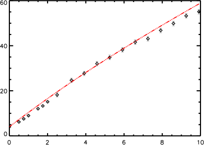
                 CME 18                                                             CME 36

Figure 1.: The observed height-time data is shown with diamonds. The red dash-dotted line is the drag model solution when it is initiated from the first observed height, $h_{0}$. CME 18 refers to the event on 22 Oct. 2011, with initial speed $\sim$ 1276 km s^-1 and CME 36 represents an event on 29 September 2013 with an initial speed $\sim$ 1217 km s^-1. Both these events are fast CMEs.fig1

       

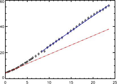
                  CME 8                                                             CME 29

Figure 2.: The observed height-time data is shown with diamonds. The red dash-dotted line is the drag model solution when it is initiated from the first observed height $h_{0}$. The blue solid line shows the predicted height-time trajectory when the drag model is initiated from height $\widetilde{h}_{0}$. CME 8 refers to the event on 24 January 2011, with initial speed $\sim$ 276 km s^-1. CME 29 represents an event on 05 October 2012 with an initial speed $\sim$ 461 km s^-1. Both CMEs 8 and 29 are slow CMEs.fig2

         

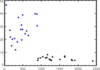
Figure 3.: Plot of initiation height ($\widetilde{h}_{0}$) and $Fall\,\%$ versus the CME initial speed. Left panel shows the quantity $\widetilde{h}_{0}$ (from where solar wind drag dominates) as a function of CME initial velocity, $v_{0}$. The right panel depicts the percentage fall in the Lorentz force from its peak value to its value at $\widetilde{h}_{0}$ (%) as a function of CME initial velocity, $v_{0}$. Symbols in blue represent slow CMEs (i.e. $v_{0}<900$ km s^-1) and symbols in black represent fast CMEs ($v_{0}>900$ km s^-1). See Table tbl2 for the values in the figure.

fig33

       

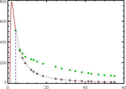
                  CME 18                                                             CME 36

Figure 4.: Comparison of Lorentz and drag forces for fast CMEs. The open diamond symbols represent the Lorentz force values derived observationally starting from $h_{0}$. The red solid line indicates the Lorentz force values for heights between $h_{eq}$ and $h_{0}$. The filled green circles represent the absolute value of the solar wind drag force. The dashed vertical line (blue) indicates the height $\widetilde{h}_{0}$ at which the solar wind drag force takes over. This height is the first observation point for both CMEs 18 and 36. For CME 18 $\widetilde{h}_{0}\sim 4$ R_⊙, while for CME 36 $\widetilde{h}_{0}\sim 4.9$ R_⊙. fig3

       

                CME 8                                                             CME 29

Figure 5.: Comparison of Lorentz and drag forces for the slow CMEs (8 and 29). The symbols and linestyles are the same as in Figure fig3.fig4

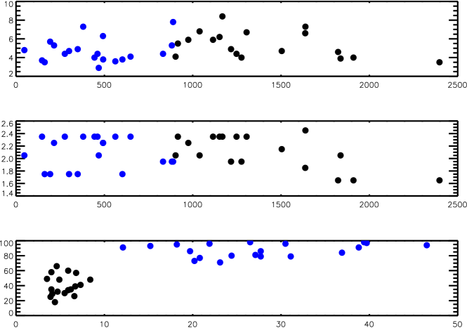
Figure 6.: Summary of some of the results in Table tbl2. The blue circles represent quantities for slow CMEs and black circles represent fast CMEs. Panels a and b plot the quantities $h_{0}$ and $h_{peak}$ respectively as a function of CME initial velocity, $v_{0}$. Panel c shows the percentage decrease, $Fall\,\%$ in Lorentz force (between its peak and $\widetilde{h}_{0}$) as a function of $\widetilde{h_{0}}$ for both slow (blue circles) and fast (black circles) CMEs. fig7

       

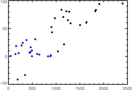
                (a)                                                                          (b)

Figure 7.: Plot of the relative difference between the two forces at $\widetilde{h}_{0}$ and variation of the drag force magnitude versus CME initial velocity. Panel a shows the percentage difference between drag and Lorentz forces as a function of CME initial velocity, $v_{0}$. $F_{\rm diff}$ is calculated at 40 R_⊙ for all CMEs except CME 11, for which it is evaluated at 50 R_⊙. Panel b shows the absolute value of drag force at $\widetilde{h}_{0}$ for all CMEs with respect to the CME initial velocity, $v_{0}$. Details are described in the text. The blue circles represent slow CMEs and the black ones represent fast CMEs. fig8

References

- Bein et al. (2011) Bein, B.M., Berkebile-Stoiser, S., Veronig, A.M., Temmer, M., Muhr, N., Kienreich, I., et al.: 2011, Impulsive Acceleration of Coronal Mass Ejections. I. Statistics and Coronal Mass Ejection Source Region Characteristics. ApJ 738, 191. DOI. ADS.
- Bosman et al. (2012) Bosman, E., Bothmer, V., Nisticò, G., Vourlidas, A., Howard, R.A., Davies, J.A.: 2012, Three-Dimensional Properties of Coronal Mass Ejections from STEREO/SECCHI Observations. Sol. Phys. 281, 167. DOI. ADS.
- Bothmer and Daglis (2007) Bothmer, V., Daglis, I.A.: 2007, Space Weather – Physics and Effects. DOI. ADS.
- Brueckner et al. (1995) Brueckner, G.E., Howard, R.A., Koomen, M.J., Korendyke, C.M., Michels, D.J., Moses, J.D., et al.: 1995, The Large Angle Spectroscopic Coronagraph (LASCO). Sol. Phys. 162, 357. DOI. ADS.
- Cargill (2004) Cargill, P.J.: 2004, On the Aerodynamic Drag Force Acting on Interplanetary Coronal Mass Ejections. Sol. Phys. 221, 135. DOI. ADS.
- Carley, McAteer, and Gallagher (2012) Carley, E.P., McAteer, R.T.J., Gallagher, P.T.: 2012, Coronal Mass Ejection Mass, Energy, and Force Estimates Using STEREO. ApJ 752, 36. DOI. ADS.
- Chen (1989) Chen, J.: 1989, Effects of toroidal forces in current loops embedded in a background plasma. ApJ 338, 453. DOI. ADS.
- Chen (1996) Chen, J.: 1996, Theory of prominence eruption and propagation: Interplanetary consequences. J. Geophys. Res. 101, 27499. DOI. ADS.
- Chen and Kunkel (2010) Chen, J., Kunkel, V.: 2010, Temporal and Physical Connection Between Coronal Mass Ejections and Flares. ApJ 717, 1105. DOI. ADS.
- Chen et al. (1997) Chen, J., Howard, R.A., Brueckner, G.E., Santoro, R., Krall, J., Paswaters, S.E., et. al.: 1997, Evidence of an Erupting Magnetic Flux Rope: LASCO Coronal Mass Ejection of 1997 April 13. ApJ 490, L191. DOI. ADS.
- Emslie et al. (2012) Emslie, A.G., Dennis, B.R., Shih, A.Y., Chamberlin, P.C., Mewaldt, R.A., Moore, C.S., et al.: 2012, Global Energetics of Thirty-eight Large Solar Eruptive Events. ApJ 759, 71. DOI. ADS.
- Forbes (2000) Forbes, T.G.: 2000, A review on the genesis of coronal mass ejections. J. Geophys. Res. 105, 23153. DOI. ADS.
- Forbes and Isenberg (1991) Forbes, T.G., Isenberg, P.A.: 1991, A catastrophe mechanism for coronal mass ejections. ApJ 373, 294. DOI. ADS.
- Fry et al. (2003) Fry, C.D., Dryer, M., Smith, Z., Sun, W., Deehr, C.S., Akasofu, S.-I.: 2003, Forecasting solar wind structures and shock arrival times using an ensemble of models. J. Geophys. Res. 108, 1070. DOI. ADS.
- Gopalswamy (2013) Gopalswamy, N.: 2013, STEREO and SOHO contributions to coronal mass ejection studies: Some recent results. In: Astron. Soc. India C.S. 10. ADS.
- Gosling et al. (1991) Gosling, J.T., McComas, D.J., Phillips, J.L., Bame, S.J.: 1991, Geomagnetic activity associated with earth passage of interplanetary shock disturbances and coronal mass ejections. J. Geophys. Res. 96, 7831. DOI. ADS.
- Howard et al. (2008) Howard, R.A., Moses, J.D., Vourlidas, A., Newmark, J.S., Socker, D.G., Plunkett, S.P., et al.: 2008, Sun Earth Connection Coronal and Heliospheric Investigation (SECCHI). Space Sci. Rev. 136, 67. DOI. ADS.
- Isenberg and Forbes (2007) Isenberg, P.A., Forbes, T.G.: 2007, A Three-dimensional Line-tied Magnetic Field Model for Solar Eruptions. ApJ 670, 1453. DOI. ADS.
- Jin et al. (2017) Jin, M., Manchester, W.B., van der Holst, B., Sokolov, I., Tóth, G., Mullinix, R.E., Taktakishvili, A., Chulaki, A., Gombosi, T.I.: 2017, Data-constrained Coronal Mass Ejections in a Global Magnetohydrodynamics Model. ApJ 834, 173. DOI. ADS.
- Kaiser et al. (2008) Kaiser, M.L., Kucera, T.A., Davila, J.M., St. Cyr, O.C., Guhathakurta, M., Christian, E.: 2008, The STEREO Mission: An Introduction. Space Sci. Rev. 136, 5. DOI. ADS.
- Kliem and Török (2006) Kliem, B., Török, T.: 2006, Torus Instability. Phys. Rev. Lett. 96(25), 255002. DOI. ADS.
- Kliem et al. (2014) Kliem, B., Lin, J., Forbes, T.G., Priest, E.R., Török, T.: 2014, Catastrophe versus Instability for the Eruption of a Toroidal Solar Magnetic Flux Rope. ApJ 789, 46. DOI. ADS.
- Kumar and Rust (1996) Kumar, A., Rust, D.M.: 1996, Interplanetary magnetic clouds, helicity conservation, and current-core flux-ropes. J. Geophys. Res. 101, 15667. DOI. ADS.
- Lee et al. (2013) Lee, C.O., Arge, C.N., Odstrčil, D., Millward, G., Pizzo, V., Quinn, J.M., et al.: 2013, Ensemble Modeling of CME Propagation. Sol. Phys. 285, 349. DOI. ADS.
- Lugaz et al. (2007) Lugaz, N., Manchester, W.B. IV, Roussev, I.I., Tóth, G., Gombosi, T.I.: 2007, Numerical Investigation of the Homologous Coronal Mass Ejection Events from Active Region 9236. ApJ 659, 788. DOI. ADS.
- Mays et al. (2015) Mays, M.L., Taktakishvili, A., Pulkkinen, A., MacNeice, P.J., Rastätter, L., Odstrcil, D., Jian, L.K., Richardson, I.G., LaSota, J.A., Zheng, Y., Kuznetsova, M.M.: 2015, Ensemble Modeling of CMEs Using the WSA-ENLIL+Cone Model. Sol. Phys. 290, 1775. DOI. ADS.
- McKenna-Lawlor et al. (2006) McKenna-Lawlor, S.M.P., Dryer, M., Kartalev, M.D., Smith, Z., Fry, C.D., Sun, W., et al.: 2006, Near real-time predictions of the arrival at Earth of flare-related shocks during Solar Cycle 23. J. Geophys. Res. 111, A11103. DOI. ADS.
- Mishra and Srivastava (2013) Mishra, W., Srivastava, N.: 2013, Estimating the Arrival Time of Earth-directed Coronal Mass Ejections at in Situ Spacecraft Using COR and HI Observations from STEREO. ApJ 772, 70. DOI. ADS.
- Rollett et al. (2016) Rollett, T., Möstl, C., Isavnin, A., Davies, J.A., Kubicka, M., Amerstorfer, U.V., et al.: 2016, ElEvoHI: A Novel CME Prediction Tool for Heliospheric Imaging Combining an Elliptical Front with Drag-based Model Fitting. ApJ 824, 131. DOI. ADS.
- Sachdeva et al. (2015) Sachdeva, N., Subramanian, P., Colaninno, R., Vourlidas, A.: 2015, CME Propagation: Where does Aerodynamic Drag ’Take Over’? ApJ 809, 158. DOI. ADS.
- Shafranov (1966) Shafranov, V.D.: 1966, Plasma Equilibrium in a Magnetic Field. Rev. Plasma Phys. 2, 103. ADS.
- Subramanian and Vourlidas (2007) Subramanian, P., Vourlidas, A.: 2007, Energetics of solar coronal mass ejections. A&A 467, 685. DOI. ADS.
- Subramanian, Lara, and Borgazzi (2012) Subramanian, P., Lara, A., Borgazzi, A.: 2012, Can solar wind viscous drag account for coronal mass ejection deceleration? Geophys. Res. Lett. 39, L19107. DOI. ADS.
- Taktakishvili et al. (2009) Taktakishvili, A., Kuznetsova, M., MacNeice, P., Hesse, M., Rastätter, L., Pulkkinen, A., et al.: 2009, Validation of the coronal mass ejection predictions at the Earth orbit estimated by ENLIL heliosphere cone model. Space Weather 7, S03004. DOI. ADS.
- Temmer and Nitta (2015) Temmer, M., Nitta, N.V.: 2015, Interplanetary Propagation Behavior of the Fast Coronal Mass Ejection on 23 July 2012. Sol. Phys. 290, 919. DOI. ADS.
- Temmer et al. (2012) Temmer, M., Vršnak, B., Rollett, T., Bein, B., de Koning, C.A., Liu, Y., Bosman, E., Davies, J.A., Möstl, C., Žic, T., Veronig, A.M., Bothmer, V., Harrison, R., Nitta, N., Bisi, M., Flor, O., Eastwood, J., Odstrcil, D., Forsyth, R.: 2012, Characteristics of Kinematics of a Coronal Mass Ejection during the 2010 August 1 CME-CME Interaction Event. ApJ 749, 57. DOI. ADS.
- Thernisien (2011) Thernisien, A.: 2011, Implementation of the Graduated Cylindrical Shell Model for the Three-dimensional Reconstruction of Coronal Mass Ejections. ApJS 194, 33. DOI. ADS.
- Thernisien, Vourlidas, and Howard (2009) Thernisien, A., Vourlidas, A., Howard, R.A.: 2009, Forward Modeling of Coronal Mass Ejections Using STEREO/SECCHI Data. Sol. Phys. 256, 111. DOI. ADS.
- Thernisien, Howard, and Vourlidas (2006) Thernisien, A.F.R., Howard, R.A., Vourlidas, A.: 2006, Modeling of Flux Rope Coronal Mass Ejections. ApJ 652, 763. DOI. ADS.
- Tóth et al. (2007) Tóth, G., de Zeeuw, D.L., Gombosi, T.I., Manchester, W.B., Ridley, A.J., Sokolov, I.V., et al.: 2007, Sun-to-thermosphere simulation of the 28-30 October 2003 storm with the Space Weather Modeling Framework. Space Weather 5, 06003. DOI. ADS.
- Vršnak (2006) Vršnak, B.: 2006, Forces governing coronal mass ejections. Adv. Space Res. 38, 431. DOI. ADS.
- Vršnak et al. (2010) Vršnak, B., Žic, T., Falkenberg, T.V., Möstl, C., Vennerstrom, S., Vrbanec, D.: 2010, The role of aerodynamic drag in propagation of interplanetary coronal mass ejections. A&A 512, A43. DOI. ADS.
- Vršnak et al. (2014) Vršnak, B., Temmer, M., Žic, T., Taktakishvili, A., Dumbović, M., Möstl, C., et al.: 2014, Heliospheric Propagation of Coronal Mass Ejections: Comparison of Numerical WSA-ENLIL+Cone Model and Analytical Drag-based Model. ApJS 213, 21. DOI. ADS.
- Wang, Zhang, and Shen (2009) Wang, Y., Zhang, J., Shen, C.: 2009, An analytical model probing the internal state of coronal mass ejections based on observations of their expansions and propagations. J. Geophys. Res. 114, A10104. DOI. ADS.
- Wood et al. (1997) Wood, B.E., Karovska, M., Cook, J.W., Brueckner, G.E., Howard, R.A.: 1997, LASCO Observations of Variability in the Quiescent Solar Corona. In: Bull. Amer. Astron. Soc. 29, 1321. ADS.
- Wu et al. (2007) Wu, C.-C., Fry, C.D., Wu, S.T., Dryer, M., Liou, K.: 2007, Three-dimensional global simulation of interplanetary coronal mass ejection propagation from the Sun to the heliosphere: Solar event of 12 May 1997. J. Geophys. Res. 112, A09104. DOI. ADS.
- Zhang and Dere (2006) Zhang, J., Dere, K.P.: 2006, A Statistical Study of Main and Residual Accelerations of Coronal Mass Ejections. ApJ 649, 1100. DOI. ADS.
- Zhang et al. (2001) Zhang, J., Dere, K.P., Howard, R.A., Kundu, M.R., White, S.M.: 2001, On the Temporal Relationship between Coronal Mass Ejections and Flares. ApJ 559, 452. DOI. ADS.
- Zhao and Dryer (2014) Zhao, X., Dryer, M.: 2014, Current status of CME/shock arrival time prediction. Space Weather 12, 448. DOI. ADS.